economics of growth and globalization

Economics of Growth and Globalization

Lecture 5: Growth Models

Alessio Moro, University of Cagliari

November 29, 2017

Lecture 5: Growth Models Economics of Growth and Globalization

Intro

In this lecture we will revise the growth model of exogenousgrowth.

In this model, GDP growth is driven by an exogenoustechnological progress that grows at a certain rate.

Next, we will modify the model to allow for multiple sectors.

Lecture 5: Growth Models Economics of Globalization 2 of 24

Kaldor Facts (Kaldor, 1961)

1 Labor productivity (Y/L) has grown at a sustained rate

2 Capital per worker (K/L) has also grown at a sustained rate

3 The real interest rate, or return on capital, has been stable.

4 The ratio of capital to output (K/Y) has also been stable.

5 Capital and labor have captured stable shares of nationalincome.

6 Among the fastest growing countries in the world there isappreciable variation in the rate of growth.


One-sector exogenous growth model: centralized solution

There is a representative household with preferences

∞∑t=0

βt logCt .

with the subjective discount factor β < 1. The objective of the householdis to maximize the discounted sum of an infinite stream ofconsumption. These preferences imply that consumption in time periodscloser to zero are given more weight than periods further away.

The household is endowed with one unit of labor that shesupplies inelastically in the market.

There is a representative firm producing the output good usingcapital and labor

Yt = K θt (AtNt)

1−θ,


Two-sector exogenous growth model: centralized solution

The evolution of the capital stock in the economy is

Kt+1 = Kt(1− δ) + Xt

with the depreciation rate 0 < δ < 1. Here Xt is the amount of outputthat is invested to produce new capital.


Social planner

Assume that there is a benevolent social planner that is willing tomaximize the utility of the household.

This planner will allocate resources efficiently to do this. Theresource constraint of the planner is then

Ct + Xt = Yt

orCt + Kt+1 = K θ

t (AtNt)1−θ + Kt(1− δ)


Lagrangean

The maximization problems requires to choose consumption Ct

and capital in the next period Kt+1.

Labor is supplied inelastically so there is no decision on it.

The Lagrangean of the planner is

L =∞∑t=0

βt logCt +∞∑t=0

µt

[K θt (AtNt)

1−θ + Kt(1− δ)− Ct − Kt+1

]The planner maximizes with respect to two variables, Ct and Kt+1.


FOCs

βt

Ct= µt (1)

µt+1[θK θ−1t+1 (At+1Nt+1)1−θ + (1− δ)] = µt (2)

From (1) and (2) we can get (3)

βCt [θKθ−1t+1 (At+1Nt+1)1−θ + (1− δ)] = Ct+1 (3)

which is the consumption Euler Equation.


Steady State

If technological change is zero At = At+1 = A we can find a steadystate for this economy:

In steady state all variables are constant over time, thusCt = Ct+1 = C and Kt = Kt+1 = K .

From (3)βC [θK θ−1A1−θ + (1− δ)] = C

θK θ−1A1−θ + (1− δ) = 1/β

K =θ1/(1−θ)A

(1/β − 1 + δ)1/(1−θ)


Steady State

And using the constraint of the planner we can find consumption

C + K = K θ (A)1−θ + K (1− δ)

C =θθ/(1−θ)A

(1/β − 1 + δ)θ/(1−θ)− θ1/(1−θ)Aδ

(1/β − 1 + δ)1/(1−θ)


Balanced growth path

If technological change is non-zero, but grows at a constant rate(1 + γa) = At+1/At this economy has a balanced growth path.

On a balanced growth path all variables grow at a constant rate.Consider again (3)

β

[θ

(At

Kt

)1−θ

+ (1− δ)

]=

Ct+1

Ct(4)

If Ct+1/Ct=1 + γc is constant it must be that A and K grow atthe same rate.

β

[θ

(At(1 + γa)

Kt(1 + γk)

)1−θ

+ (1− δ)

]= (1 + γc)

Thus γk=γa.



How about the growth rate of Y and C?

Consider the production function and take logs

logYt = θlogKt + (1− θ)logAt ,

Now take the difference between two periods t+1 and t

logYt+1 − logYt = θ (logKt+1 − logKt) + (1− θ) (logAt+1 − logAt) ,

log (Yt+1/Yt) = θlog (Kt+1/Kt) + (1− θ)log (At+1/At) ,

log(1 + γy ) = θlog(1 + γk) + (1− θ)log(1 + γa) ,

log(1 + γy ) = θlog(1 + γa) + (1− θ)log(1 + γa) ,

log(1 + γy ) = log(1 + γa)

γy = γa .

Thus also Y grows at the same rate as A.



Consider now the feasibility constraint

Ct + Kt+1 = K θt (At)

1−θ + Kt(1− δ)

after one period

(1 + γc)Ct + (1 + γa)Kt+1 = (1 + γa)K θt (At)

1−θ +Kt(1 + γa)(1− δ)

The only way for this constraint to hold after one period is thatγc=γa. Thus in this economy all variables grow at the same rate,which is the rate of technological change.


Decentralized equilibrium

In a decentralized equilibrium there is no social planner.

The household takes market prices as given and makes optimaldecisions to maximize utility.

The firm takes market prices as given and makes optimaldecisions to maximize profits.

The interaction of household and firm determines the marketequilibrium.


Household

There is a representative household with preferences

∞∑t=0

βt logCt .

with the subjective discount factor β < 1.

The household is endowed with one unit of labor that she suppliesinelastically in the market.

The household also holds the capital stock of the economy.She uses capital to move resources from the present to the future.Thus, the budget constraint of the household is

Ct + Kt+1 = wt + Kt(1 + rt − δ)

Here wt is the wage rate received by the household for providinglabor in the market and rt is the rental rate that the householdreceives by renting capital to firms.


Household

The Lagrangean of the household is

L =∞∑t=0

βt logCt +∞∑t=0

µt [wt + Kt(1 + rt − δ)− Ct − Kt+1] .

The household maximizes with respect to two variables, Ct andKt+1.


Firm

There is a representative firm producing the output good usingcapital and labor

Yt = kθt (AtNt)1−θ

,

Objective of the firm is to maximize profits by choosing theamount of capital and labor to use in production.

Note that we assume perfect competition. In PC firms takeprices as given. Assuming also constant returns to scale impliesthat the number of firms is irrelevant and we can assume only onerepresentative firm.

The representative firm then solves

maxNt ,Kt

Π = maxNt ,Kt

[ptk

θt (AtNt)

1−θ − wtNt − rtkt].

Note that the problem of the firm is static (and no constraints),while that of the consumer is dynamic (and with a constraint).


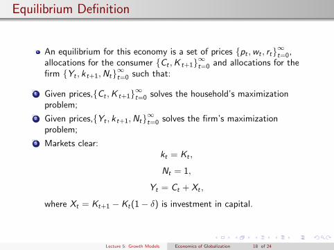
Equilibrium Definition

An equilibrium for this economy is a set of prices {pt ,wt , rt}∞t=0,allocations for the consumer {Ct ,K t+1}∞t=0 and allocations for thefirm {Yt , k t+1,Nt}∞t=0 such that:

1 Given prices,{Ct ,K t+1}∞t=0 solves the household’s maximizationproblem;

2 Given prices,{Yt , k t+1,Nt}∞t=0 solves the firm’s maximizationproblem;

3 Markets clear:kt = Kt ,

Nt = 1,

Yt = Ct + Xt ,

where Xt = Kt+1 − Kt(1− δ) is investment in capital.


Firm FOCs

rt = ptθ

(Kt

Nt

)θ−1A1−θt (5)

wt = pt(1− θ)

(Kt

Nt

)θA1−θt (6)

Using (5) and (6) we obtain

Kt

Nt=

θ

1− θwt

rt(7)


Household FOCs

βt

Ct= µt (8)

µt+1[rt+1 + (1− δ)] = µt (9)

From (8) and (9) we can get (10)

βCt [rt+1 + (1− δ)] = Ct+1 (10)

which is the Euler Equation for the household.


Solving the model

By setting pt = 1as the numeraire, and considering that inequilibrium it must be Nt = 1

rt = θK θ−1t A1−θ

t

We can then substitute in the Euler equation to obtain

βCt [θKθ−1t+1 A

1−θt+1 + (1− δ)] = Ct+1 (11)

which is the same equation that we had in the centralized problem.


Solving the model

Consider now the budget constraint of the consumer

Ct + Kt+1 = wt + rtKt + Kt(1− δ)

Substitute for wt and rt from the firm’s FOCs (again settingpt = 1as the numeraire, and considering that in equilibrium it mustbe Nt = 1)

Ct + Kt+1 = (1− θ)K θt A

1−θt + θK θ−1

t A1−θt Kt + Kt(1− δ)

Ct + Kt+1 = K θt A

1−θt + Kt(1− δ)

orCt + Kt+1 = Yt + Kt(1− δ)

which is the constraint of the social planner in the centralizedsolution.


Solving the model

Finally, we determine the evolution of the interest rate along thebalanced growth path. Recall that:

rt = θ

(Kt

At

)θ−1As K and A grow at the same rate, the interest rate is constant. Tosee this compute rt+1

rt+1 = θ

(Kt(1 + γa)

At(1 + γa)

)θ−1= θ

(Kt

At

)θ−1= rt .


Conclusions

We proved that the centralized and the market solutions areequivalent.

This is due to the first welfare theorem: every competitiveequilibrium is Pareto efficient.

The exogenous growth model satisfies the Kaldor facts.


economics of growth and globalization

Documents