economics 266: international trade | lecture 8:...
TRANSCRIPT
Economics 266: International Trade— Lecture 8: Increasing Returns to Scale and
Monopolistic Competition (Theory) —
Stanford Econ 266 (Donaldson)
Winter 2016 (lecture 8)
Stanford Econ 266 (Donaldson) IRTS and MC Winter 2016 (lecture 8) 1 / 36

Today’s Plan
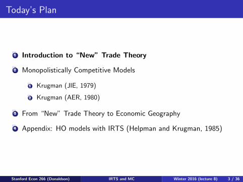
1 Introduction to “New” Trade Theory
2 Monopolistically Competitive Models
1 Krugman (JIE, 1979)
2 Krugman (AER, 1980)
3 From “New” Trade Theory to Economic Geography
4 Appendix: HO models with IRTS (Helpman and Krugman, 1985)
Stanford Econ 266 (Donaldson) IRTS and MC Winter 2016 (lecture 8) 2 / 36
Today’s Plan
1 Introduction to “New” Trade Theory
2 Monopolistically Competitive Models
1 Krugman (JIE, 1979)
2 Krugman (AER, 1980)
3 From “New” Trade Theory to Economic Geography
4 Appendix: HO models with IRTS (Helpman and Krugman, 1985)
Stanford Econ 266 (Donaldson) IRTS and MC Winter 2016 (lecture 8) 3 / 36

“New” (c. 1980s) Trade TheoryWhat’s wrong with neoclassical trade theory?
In a neoclassical world, differences in relative autarky prices—due todifferences in technology, factor endowments, or preferences—are theonly rationale for trade.
This suggests that:
1 “Different” countries should trade more.
2 “Different” countries should specialize in “different” goods.
In the real world, however, we observe that:
1 The bulk of world trade is between “similar” countries.
2 These countries tend to trade “similar” goods.
Stanford Econ 266 (Donaldson) IRTS and MC Winter 2016 (lecture 8) 4 / 36
“New” (c. 1980s) Trade TheoryWhy Increasing Returns to Scale (IRTS)?
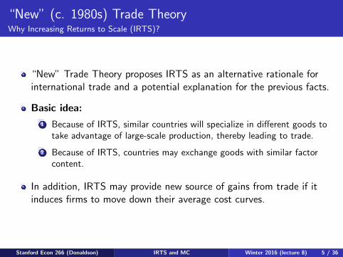
“New” Trade Theory proposes IRTS as an alternative rationale forinternational trade and a potential explanation for the previous facts.
Basic idea:
1 Because of IRTS, similar countries will specialize in different goods totake advantage of large-scale production, thereby leading to trade.
2 Because of IRTS, countries may exchange goods with similar factorcontent.
In addition, IRTS may provide new source of gains from trade if itinduces firms to move down their average cost curves.
Stanford Econ 266 (Donaldson) IRTS and MC Winter 2016 (lecture 8) 5 / 36
“New” Trade TheoryHow to model increasing returns to scale?
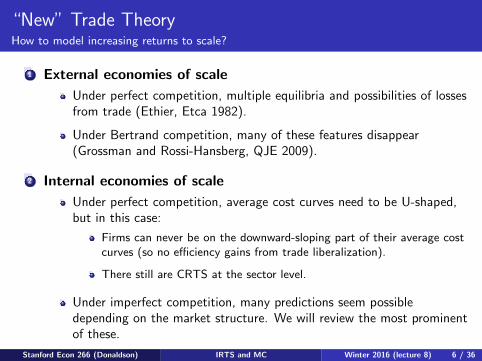
1 External economies of scale
Under perfect competition, multiple equilibria and possibilities of lossesfrom trade (Ethier, Etca 1982).
Under Bertrand competition, many of these features disappear(Grossman and Rossi-Hansberg, QJE 2009).
2 Internal economies of scale
Under perfect competition, average cost curves need to be U-shaped,but in this case:
Firms can never be on the downward-sloping part of their average costcurves (so no efficiency gains from trade liberalization).
There still are CRTS at the sector level.
Under imperfect competition, many predictions seem possibledepending on the market structure. We will review the most prominentof these.
Stanford Econ 266 (Donaldson) IRTS and MC Winter 2016 (lecture 8) 6 / 36

Today’s Plan
1 Introduction to “New” Trade Theory
2 Monopolistically Competitive Models
1 Krugman (JIE, 1979)
2 Krugman (AER, 1980)
3 From “New” Trade Theory to Economic Geography
4 Appendix: HO models with IRTS (Helpman and Krugman, 1985)
Stanford Econ 266 (Donaldson) IRTS and MC Winter 2016 (lecture 8) 7 / 36

Monopolistic CompetitionTrade economists’ preferred assumption about market structure
Monopolistic competition, formalized by Dixit and Stiglitz (1977), isthe most common market structure assumption among “new” trademodels (as in many other fields that sought to model internal IRTS).
It provides a very mild departure from imperfect competition, butopens up a rich set of new issues.
Classical examples:
Krugman (1979): IRTS as a new rationale for international trade.
Krugman (1980): Home market effect in the presence of trade costs.
Helpman and Krugman (1985): Inter- and intra-industry trade united.
Stanford Econ 266 (Donaldson) IRTS and MC Winter 2016 (lecture 8) 8 / 36
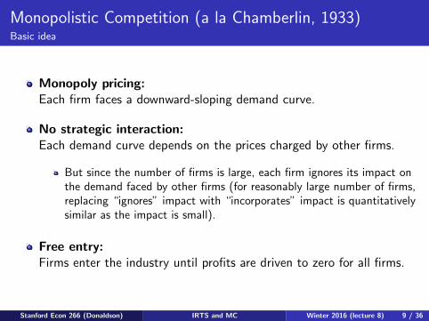
Monopolistic Competition (a la Chamberlin, 1933)Basic idea
Monopoly pricing:Each firm faces a downward-sloping demand curve.
No strategic interaction:Each demand curve depends on the prices charged by other firms.
But since the number of firms is large, each firm ignores its impact onthe demand faced by other firms (for reasonably large number of firms,replacing “ignores” impact with “incorporates” impact is quantitativelysimilar as the impact is small).
Free entry:Firms enter the industry until profits are driven to zero for all firms.
Stanford Econ 266 (Donaldson) IRTS and MC Winter 2016 (lecture 8) 9 / 36

Monopolistic CompetitionGraphical analysis
Monopolistic CompetitionGraphical analysis
MR
q
p AC
MC
D
Stanford Econ 266 (Donaldson) IRTS and MC Winter 2016 (lecture 8) 10 / 36
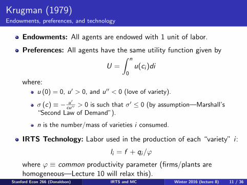
Krugman (1979)Endowments, preferences, and technology
Endowments: All agents are endowed with 1 unit of labor.
Preferences: All agents have the same utility function given by
U =
∫ n
0u(ci )di
where:
u (0) = 0, u′ > 0, and u′′ < 0 (love of variety).
σ (c) ≡ − u′
cu′′ > 0 is such that σ′ ≤ 0 (by assumption—Marshall’s“Second Law of Demand”).
n is the number/mass of varieties i consumed.
IRTS Technology: Labor used in the production of each “variety” i :
li = f + qi/ϕ
where ϕ ≡ common productivity parameter (firms/plants arehomogeneous—Lecture 10 will relax this).
Stanford Econ 266 (Donaldson) IRTS and MC Winter 2016 (lecture 8) 11 / 36

Krugman (1979)Equilibrium conditions
1 Consumer maximization:
pi = λ−1u′ (ci )
2 Profit maximization:
pi =
[σ (ci )
σ (ci )− 1
]·(w
ϕ
)3 Free entry: (
pi −w
ϕ
)qi = wf
4 Good and labor market clearing:
qi = Lci
L = nf +
∫ n
0
qiϕdi
Stanford Econ 266 (Donaldson) IRTS and MC Winter 2016 (lecture 8) 12 / 36
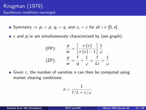
Krugman (1979)Equilibrium conditions rearranged
Symmetry ⇒ pi = p, qi = q, and ci = c for all i ∈ [0, n] .
c and p/w are simultaneously characterized by (see graph):
(PP):p
w=
[σ (c)
σ (c)− 1
]1
ϕ
(ZP):p
w=
f
q+
1
ϕ=
f
Lc+
1
ϕ
Given c , the number of varieties n can then be computed usingmarket clearing conditions:
n =1
f /L + c/ϕ
Stanford Econ 266 (Donaldson) IRTS and MC Winter 2016 (lecture 8) 13 / 36

Krugman (1979)
Graphical analysis; PP is upward-sloping thanks to assumption thatelasticity of substitution is falling
Krugman (1979)Graphical analysis; PP is upward sloping thanks to assumption that elasticity ofsubstitution is falling
(p/w)0
c0
Z
c
p/wP
PZ
Stanford Econ 266 (Donaldson) IRTS and MC Winter 2016 (lecture 8) 14 / 36
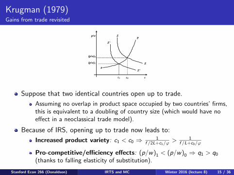
Krugman (1979)Gains from trade revisited
Krugman (1979)Gains from trade revisited
(p/w)0
c1 c0
Z’
Z
c
p/wP
Z’
PZ(p/w)1
• Suppose that two identical countries open up to trade.• This is equivalent to a doubling of country size (which would have noeffect in a neoclassical trade model).
• Because of IRS, opening up to trade now leads to:• Increased product variety: c1 < c0 ⇒ 1
f /2L+c1/ϕ >1
f /L+c0/ϕ
• Pro-competitive/effi ciency effects: (p/w)1 < (p/w)0 ⇒ q1 > q0(thanks to falling elasticity of substitution).
Suppose that two identical countries open up to trade.
Assuming no overlap in product space occupied by two countries’ firms,this is equivalent to a doubling of country size (which would have noeffect in a neoclassical trade model).
Because of IRS, opening up to trade now leads to:
Increased product variety: c1 < c0 ⇒ 1f /2L+c1/ϕ
> 1f /L+c0/ϕ
Pro-competitive/efficiency effects: (p/w)1 < (p/w)0 ⇒ q1 > q0(thanks to falling elasticity of substitution).
Stanford Econ 266 (Donaldson) IRTS and MC Winter 2016 (lecture 8) 15 / 36

Today’s Plan
1 Introduction to “New” Trade Theory
2 Monopolistically Competitive Models
1 Krugman (JIE, 1979)
2 Krugman (AER, 1980)
3 From “New” Trade Theory to Economic Geography
4 Appendix: HO models with IRTS (Helpman and Krugman, 1985)
Stanford Econ 266 (Donaldson) IRTS and MC Winter 2016 (lecture 8) 16 / 36
CES PreferencesTrade economists’ preferred demand system
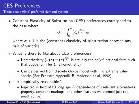
Constant Elasticity of Substitution (CES) preferences correspond tothe case where:
U =
∫ n
0(ci )
σ−1σ di ,
where σ > 1 is the (constant) elasticity of substitution between anypair of varieties.
What is there to like about CES preferences?
Homotheticity (u (c) ≡ (c)σ−1σ is actually the only functional form such
that above form for U is homothetic).
Can be derived from discrete choice model with i.i.d extreme valueshocks (See Feenstra Appendix B, Anderson et al, 1992).
Is it empirically reasonable?
Rejected in field of IO long ago (independence of irrelevant alternativesproperty, constant markups, and other features we deemed just toounattractive).
Stanford Econ 266 (Donaldson) IRTS and MC Winter 2016 (lecture 8) 17 / 36

CES PreferencesSpecial properties of the equilibrium
Because of monopoly pricing, CES ⇒ constant markups:
p
w=
[σ
σ − 1
]1
ϕ
Because of zero profit, constant markups ⇒ constant output per firm:
p
w=
f
q+
1
ϕ
Because of market clearing, constant output per firm ⇒ constantnumber of varieties per country:
n =L
f + q/ϕ
So, gains from trade come only from access to Foreign varieties.
IRTS provide an intuitive reason for why Foreign varieties are different.But consequences of trade would now be the same if we hadmaintained CRTS with different countries producing different goods(the so-called “Armington assumption”).
Stanford Econ 266 (Donaldson) IRTS and MC Winter 2016 (lecture 8) 18 / 36
Krugman (1980)The role of trade costs
Trade costs were largely absent from neoclassical trade models.
Solving for the pattern of international specialization in the presence oftrade costs is hard.
We now explore the implications of trade costs in the presence ofIRTS.
Thanks to Dixit-Stiglitz product differentiation:1 Solving for international specialization is easy (each firm is deliberately
the only firm in the world to make its own variety).2 And this is not substantially complicated by trade costs (especially ad
valorem trade costs that don’t require factors of production or generateincome—so called ‘iceberg’ trade costs).
Stanford Econ 266 (Donaldson) IRTS and MC Winter 2016 (lecture 8) 19 / 36
Krugman (1980)The role of trade costs
Main result: “Home-market effect”
Countries will tend to export those goods for which they have relativelylarge domestic markets.
Basic idea:
Because of IRS, firms will locate in only one market.
Because of trade costs, firms prefer to locate in larger markets.
Logic is very different from neoclassical trade theory in which largerdemand tends to be associated with imports rather than exports.
Stanford Econ 266 (Donaldson) IRTS and MC Winter 2016 (lecture 8) 20 / 36
Krugman (1980)Starting point: one factor, one industry, two countries
There are two countries: Home (H) and Foreign (F ).
There is one differentiated good produced under IRTS bymonopolistically competitive firms, as in Krugman (1979).
But (unlike in more general Krugman (1979) case) preferences overvarieties are CES:
U =
∫ n
0(ci )
σ−1σ di ,
There are iceberg trade costs between countries:
In order to sell 1 unit abroad, domestic firms must ship τ > 1 units.
Stanford Econ 266 (Donaldson) IRTS and MC Winter 2016 (lecture 8) 21 / 36

Krugman (1980)Equilibrium conditions (Home Country)
1 Consumer maximization:
qH,H =wHLH
PH
(pHH/PH
)−σ, qF ,H =
wHLH
PH
(pF ,H/PH
)−σ(1)
where PH =[nH(pH,H
)1−σ+ nF
(pF ,H
)1−σ] 11−σ
.
2 Monopoly pricing:
pH,H =
[σ
σ − 1
]·(wH/ϕ
), pH,F =
[σ
σ − 1
]·(τwH/ϕ
)(2)
3 Free entry:(pH,H − wH/ϕ
)qH,H +
(pH,F − wH/ϕ
)qH,F = wH f , (3)
4 Labor market clearing:
LH = nH(f + qH,H/ϕ+ τqH,F/ϕ
)(4)
Stanford Econ 266 (Donaldson) IRTS and MC Winter 2016 (lecture 8) 22 / 36
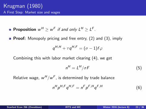
Krugman (1980)A First Step: Market size and wages
Proposition wH ≥ wF if and only LH ≥ LF .
Proof: Monopoly pricing and free entry, (2) and (3), imply
qH,H + τqH,F = (σ − 1)f ϕ
Combining this with labor market clearing (4), we get
nH = LH/σF (5)
Relative wage, wH/wF , is determined by trade balance
nHpH,FqH,F = nFpF ,HqF ,H (6)
Stanford Econ 266 (Donaldson) IRTS and MC Winter 2016 (lecture 8) 23 / 36

Krugman (1980)Market size and wages
Proof (Cont.): Combining (6) with (1) and (5) (and their Foreigncounterparts), we obtain
(wH/wF
)σ=
τ1−σ +(LH/LF
) (wH/wF
)1−σ1 + τ1−σ (LH/LF ) (wH/wF )
1−σ
Since τ1−σ < 1, this implies wH/wF ↗ in LH/LF . Propositionderives from this observation and wH/wF = 1 if LH/LF = 1
Intuition:
Everything else being equal, demand is larger in larger marketsFirms will only be active in the smaller market if they have to pay lowerwages or face softer competition, i.e. smaller number of domestic firmsBut labor supply is perfectly inelastic ⇒ number of domestic firms isfixedSo smaller market has to be associated with lower wages
Stanford Econ 266 (Donaldson) IRTS and MC Winter 2016 (lecture 8) 24 / 36

Krugman (1980)Home-Market Effect
What would happen if labor supply was perfectly elastic instead?
Suppose that we add a second industry in which a homogeneous goodis produced (NB: not just capable of being produced, but actuallyproduced in equilibrium) one-for-one for labor in both countries.
Preferences over two goods are Cobb-Douglas.
Suppose, in addition, that homogeneous good is freely traded.
Under these assumptions (“free trade in homogenous outside good”),wages are equal across countries: wH = wF .
So adjustments across countries may only come from number ofvarieties nH and nF (labor supply in the differentiated sector isendogenous).
Stanford Econ 266 (Donaldson) IRTS and MC Winter 2016 (lecture 8) 25 / 36

Krugman (1980)Home-market effect
Proposition nH/LH ≥ nF/LF if and only if LH ≥ LF .
“Home-market effect”: larger market has a disproportionately largeshare of differentiated good firms (and so will export that good).
Since wages are necessarily equal, firms will only be active in thesmaller market if they face softer competition (lower n) there.
With a little bit of algebra, one can show that (restricting attention tocases where nH > 0 and nL > 0):
nH
nF=
LH/LF − τ1−σ
1− (LH/LF ) τ1−σ
Note that ∂(nH/nF
)/∂τ1−σ > 0 if LH/LF > 1: home-market effect
is larger when trade costs are small or elasticity of substitution is large.
Stanford Econ 266 (Donaldson) IRTS and MC Winter 2016 (lecture 8) 26 / 36

Krugman (1980)NB: Krugman’s σ in this figure corresponds to τ 1−σ in our notation.
Stanford Econ 266 (Donaldson) IRTS and MC Winter 2016 (lecture 8) 27 / 36

Today’s Plan
1 Introduction to “New” Trade Theory
2 Monopolistically Competitive Models
1 Krugman (JIE, 1979)
2 Krugman (AER, 1980)
3 From “New” Trade Theory to Economic Geography
4 Appendix: HO models with IRTS (Helpman and Krugman, 1985)
Stanford Econ 266 (Donaldson) IRTS and MC Winter 2016 (lecture 8) 28 / 36

From New Trade Theory To Economic GeographyBasic Idea
Krugman (JPE 1991) added one additional assumption to Krugman(1980), which was that some workers are perfectly mobile across thetwo countries/“regions”.
Mobile workers move to where their real wage is highest.
These workers are attracted to the already larger region because of thehigher nominal wages they earn there (HME) and the wider array ofvarieties for sale there (lower price index).
This then leads to agglomeration.
Extent of agglomeration depends (very naturally) on the relativeimportance of the IRTS good in tastes, and the share of workers whoare mobile.
Stanford Econ 266 (Donaldson) IRTS and MC Winter 2016 (lecture 8) 29 / 36

From New Trade Theory To Economic GeographyBasic Idea
The result was an extremely influential model of “economicgeography”, i.e. a model in which the distribution of economicactivity across space (i.e. agglomeration) is endogenous.
See lectures 16-18 for more on this.
Stanford Econ 266 (Donaldson) IRTS and MC Winter 2016 (lecture 8) 30 / 36

Today’s Plan
1 Introduction to “New” Trade Theory
2 Monopolistically Competitive Models
1 Krugman (JIE, 1979)
2 Krugman (AER, 1980)
3 From “New” Trade Theory to Economic Geography
4 Appendix: HO models with IRTS (Helpman and Krugman,1985)
Stanford Econ 266 (Donaldson) IRTS and MC Winter 2016 (lecture 8) 31 / 36
Helpman and Krugman (1985)Inter- and intra-industry trade united
Helpman and Krugman (1985), chapters 7 and 8, offer a unifiedtheoretical framework in which to analyze inter- and intra-industrytrade.
Basic Strategy:
1 Start from the integrated equilibrium, but allow IRTS in some sectors.
2 Provide conditions such that integrated equilibrium can be replicatedunder free trade.
3 Build on the observation that each variety is only produced in onecountry, but consumed in both, to make new predictions about thestructure of trade flows when free trade replicates integratedequilibrium.
Stanford Econ 266 (Donaldson) IRTS and MC Winter 2016 (lecture 8) 32 / 36

Helpman and Krugman (1985)Back to the two-by-two-by-two world
Compared to Krugman (1979), suppose now that there are:
2 industries, i = X ,Y2 factors of production, f = l , k2 countries, North and South
Y is a “homogeneous” good produced under CRTS:
afY(w I , r I
)≡ (constant) unit factor requirements in integrated eq.
X is a “differentiated” good produced under IRTS:
afX(w I , r I , qIX
)≡ (average) unit factor requirements in integrated eq.
qIXafX(w I , r I , qIX
)≡ factor demand per firm in integrated eq.
W.l.o.g, we can set units of account s.t. qIX = 1 for all firms
Stanford Econ 266 (Donaldson) IRTS and MC Winter 2016 (lecture 8) 33 / 36

Helpman and Krugman (1985)The Integrated Equilibrium
Helpman and Krugman (1985)The Integrated Equilibrium Revisited
aX(wI,rI,qIX)nX
Slope = w/r
C
vs
vn
ks
ls
kn
On
ln
v
Os
aY(wI,rI)QY
• Taking qIX as given, integrated eq. is isomorphic to HO integrated eq.
• Pattern of inter-industry trade (and so net factor content of trade) isthe same as in HO model.
• But product differentiation + IRS lead to intra-industry trade in Y .
Taking qIX as given, integrated eq. is isomorphic to HO integrated eq.
Pattern of inter-industry trade (and so net factor content of trade) isthe same as in HO model.
But product differentiation + IRS lead to intra-industry trade in Y .
Stanford Econ 266 (Donaldson) IRTS and MC Winter 2016 (lecture 8) 34 / 36

Helpman and Krugman (1985)Trade Volumes
Intra-industry trade has strong implications for trade volumes.
In HO model (with FPE), we have seen that trade volumes do notdepend on country size.
Helpman and Krugman (1985)Trade Volumes
• Intra-industry trade has strong implications for trade volumes.
• In HO model (with FPE), we have seen that trade volumes do notdepend on country size.
ks
ls
a1(ω)
kn
On
ln
a2(ω)
y2a2(ω)
y1a1(ω)
Os
Stanford Econ 266 (Donaldson) IRTS and MC Winter 2016 (lecture 8) 35 / 36
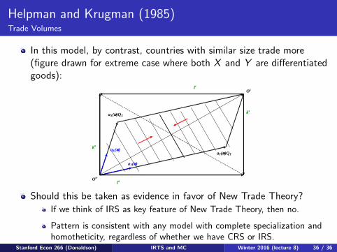
Helpman and Krugman (1985)Trade Volumes
In this model, by contrast, countries with similar size trade more(figure drawn for extreme case where both X and Y are differentiatedgoods):
Helpman and Krugman (1985)Trade Volumes
• In this model, by contrast, countries with similar size trade more(figure drawn for extreme case where both X and Y are differentiatedgoods):
ks
ls
aY(ω)
kn
On
ln
aX(ω)
aX(ω)QX
aY(ω)QY
Os
• Should this be taken as evidence in favor of New Trade Theory?• If we think of IRS as key feature of New Trade Theory, then no.
• Pattern is consistent with any model with complete specialization andhomotheticity, regardless of whether we have CRS or IRS.
Should this be taken as evidence in favor of New Trade Theory?
If we think of IRS as key feature of New Trade Theory, then no.
Pattern is consistent with any model with complete specialization andhomotheticity, regardless of whether we have CRS or IRS.
Stanford Econ 266 (Donaldson) IRTS and MC Winter 2016 (lecture 8) 36 / 36