Economics 2301

Lecture 31

Univariate Optimization

Second-Order Conditions

The second-order condition provides a sufficient condition but, as we will see, not a necessary condition, for characterizing a stationary point as a local maximum or a local minimum.

Second-Order Conditions

Local Maximum: If the second derivative of the differentiable function y=f(x) is negative when evaluated at a stationary point x* (that is, f”(x*)<0), then that stationary point represents a local maximum.

Local Minimum: If the second derivative of the differentiable function y=f(x) is positive when evaluated at a stationary point x* (that is, f”(x*)>0), then that stationary point represents a local minimum.

Second-Order Conditions for Our Examples

minimum. local a ,06;306

4303 :2 Example

maximum. local a ,012;2412

30246:1Example

2

2

2

2

2

2

dx

ydx

dx

dy

xxy

dx

ydx

dx

dy

xxy

Graph of Example 1

y=-6X2+24X-30

-120

-100

-80

-60

-40

-20

0

-3 -2 -1 0 1 2 3 4 5 6 7

x

y y

Graph of Example 2

Y=3X2-30X+4

-80

-70

-60

-50

-40

-30

-20

-10

0

10

0 1 2 3 4 5 6 7 8 9 10 11

x

y y

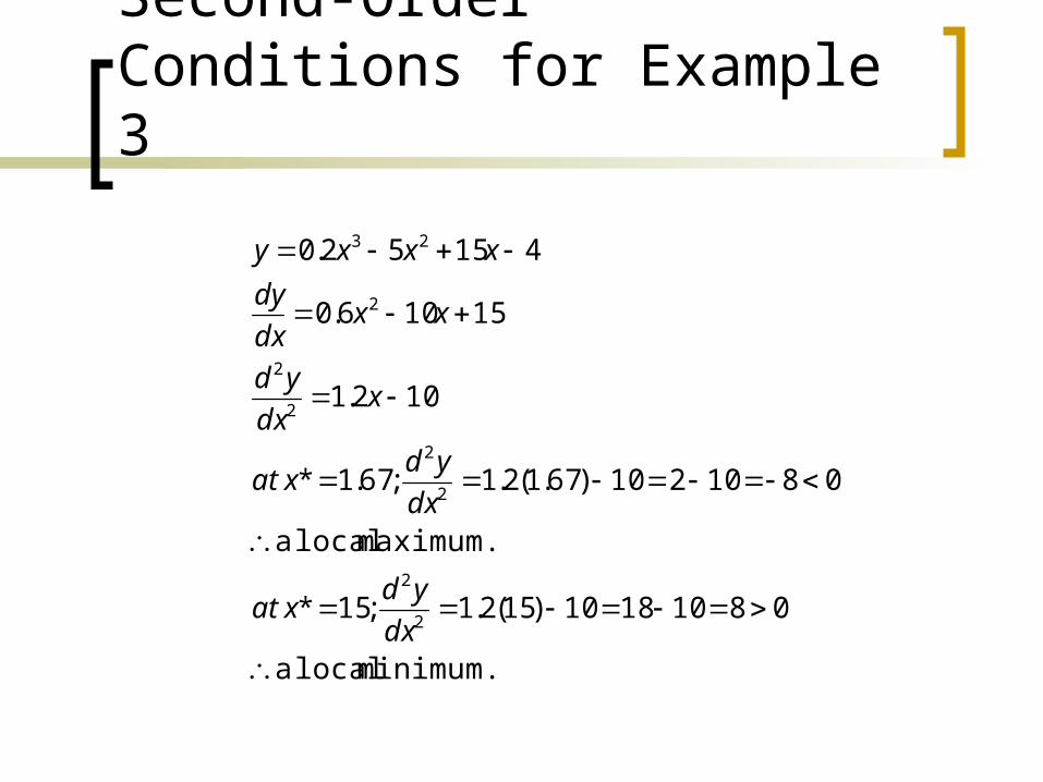
Second-Order Conditions for Example 3

minimum. local a

08101810)15(2.1;15*

maximum. local a

0810210)67.1(2.1;67.1*

102.1

15106.0

41552.0

2

2

2

2

2

2

2

23

dx

ydxat

dx

ydxat

xdx

yd

xxdx

dy

xxxy

Graph of Example 3

y=0.2X3-5X2+15X-4

-250

-200

-150

-100

-50

0

50

0 5 10 15 20 25

x

y y

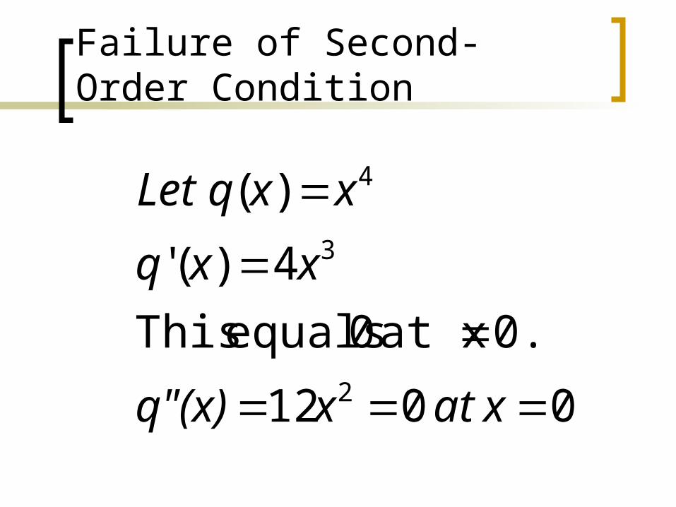
Failure of Second-Order Condition

0012

0.at x 0 equals This

4)('

)(

2

3

4

xatxq"(x)

xxq

xxqLet

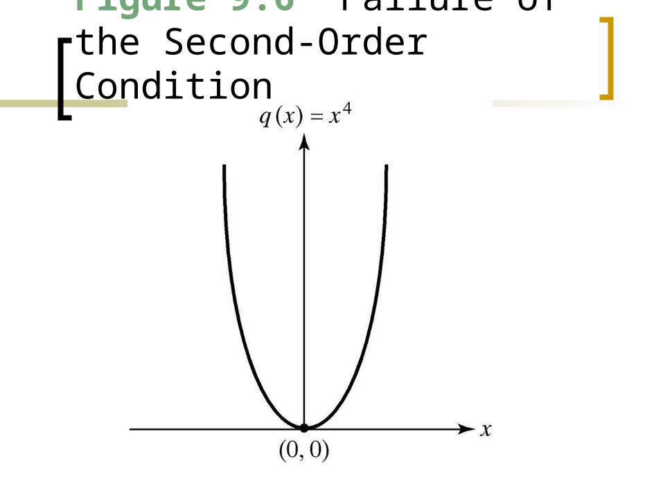
Figure 9.6 Failure of the Second-Order Condition

Stationary Point of a strictly concave function

If the function f(x) is strictly concave on the interval (m,n) and has the stationary point x*, where m<x*<n, the x* is a local maximum in that interval. If a function is strictly concave everywhere, then it has, at most, one stationary point, and that stationary point is a global maximum.

Note that example 1 satisfies this condition.

Stationary Point of a Strictly Convex Function

If the function f(x) is strictly convex on the interval (m,n) and has the stationary point x*, where m<x*<n, the x* is a local minimum in that interval. If a function is strictly convex everywhere, then it has, at most, one stationary point, and that stationary point is a global minimum.

Note that example 2 satisfies this condition.

Inflection Point

The twice-differentiable function f(x) has an inflection point at x* if and only if the sign of the second derivative switches from negative in some interval (m,x*) to positive in some interval (x*,n), in which case the function switches from concave to convex at x*, or the sign of the second derivative switches from positive in some interval (m,x*) to negative in some interval (x*,n), in which case the function switches from convex to concave at x*. Note that, in either case, m<x<n.

Example inflection point

interval. in thisconvex isfunction thehence positive,

is derivative second the8.333, ofright theTo concave.

hence negative, is derivative second the8.333, ofleft To

8.333.at x 0 equals This

102.1

15106.0

41552.0 3, exampleFor

2

2

2

23

xdx

yd

xxdx

dy

xxxy

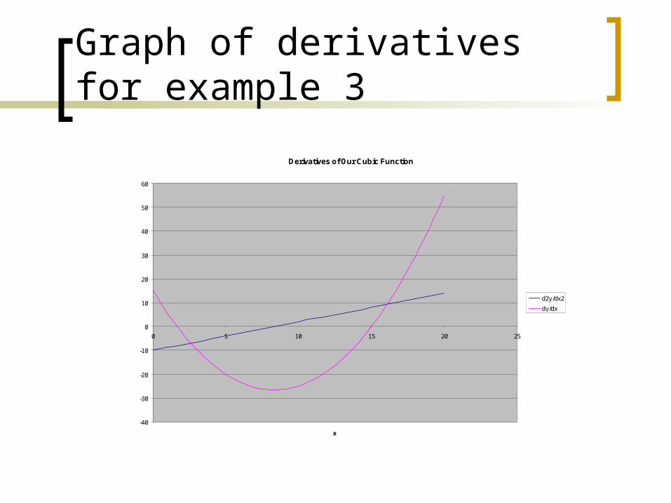
Graph of derivatives for example 3

Derivatives of Our Cubic Function

-40

-30

-20

-10

0

10

20

30

40

50

60

0 5 10 15 20 25

x

d2y/dx2

dy/dx

Graph of Example 3

y=0.2X3-5X2+15X-4

-250

-200

-150

-100

-50

0

50

0 5 10 15 20 25

x

y y

Concave

convex

Inflection point

Optimal Excise Tax

revenue.

nreservatio marginalMRR and revenue marginalMR

11

11TP

toreduceson manipulati carefulafter which

0)()(

Therefore zero. toequal Q

respect to with TR of derivative set the TR, maximize To

quantity. mequilibriuQ andunit tax per T Price,supply P

revenue, tax totalequal Let

MRRMRor

P

PdQ

dPQTP

dQ

TPdQ

dQ

dTR

whereQQ-PT)(PTR

TR

SD

Optimal excise tax rate

DMR

S

MRR

Qe

Q/T

P

Pe

Pe+Te

Optimal Timing

t.respect to with A(t) maximize want toWe

.Ve A(t)

is V of luepresent va Then the r. is basis gcompoundin continuouson

rateinterest theassume will We.comparison themake toluepresent va

itsget torevenue futureeach discount must weTherefore, ay.dollar tod

a as same thenot worth isdollar future a However, revenue. maximum

toscorrespondprofit Maximum cost. storage no is thereandfor paid is

wine that theAssume K. is luecurrent va theClearly, .KeVfunction

the toaccording with timeincreases ue which val winehasdealer A wine

rt-

t

rttrtt KeeKe

Optimal Timing Continued

22

1

2

1

2

1

2

1

4

1*

2

120

2

1

0.A since zero equalbracket in the termtheonly when zero equalsWhich

2

1

2

1

A

1

get wesides,both atedifferenti When we

tLn(K)ln(A(t))

function. luepresent vaour ofation transformlog the take will weTherefore,

function. original theas valuesame at the extremesreach tion transforma

monotonic afact that theof use make will wefunction,our maximize To

rt

rtrtrt

rtAdt

dAorrt

dt

dA

rt

Interpretation of results

r. money, holding ofcost the toequal is wine theof value

ofgrowth of rate point the stationaryour at Thus interest). of rate (ther is

gcompoundin continuousbank with in theput money ofgrowth of rate The

.2

1ln

dt

dln(V) is valueofgrowth of rate thefunction,

our valuefor Note tion.interpretaeasy an admit conditionsorder first Our

2

1

tdt

tKd

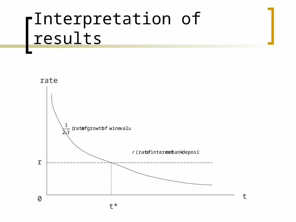
Interpretation of results

value) wineofgrowth of rate(2

1

t

t

rate

r

t*

deposits)bank on interest of (rate r

0

Second Order Condition

.*at t 0A Since

.*at t 04

1

2

1

have wezero, is last term theSince

2

1

2

1

2

1

2

3

2

1

2

2

2

1

2

1

2

1

2

2

tArtdt

dA

dt

Ad

dt

dArtrt

dt

dArtA

dt

d

dt

Ad