economic valuation of mortality risk reduction - us … valuation of mortality risk reduction: ... $...

Economic Valuation of Mortality Risk Reduction: Assessing the State of the Art for Policy Applications

PROCEEDINGS BSession IB

A Review of Current Approaches To Valuing Mortality Risks

A workshop sponsored by the US Environmental Protection Agency=s

National Center for Environmental Economics and National Center for Environmental Research

November 6, 2001 The Holiday Inn Silver Spring Hotel

8777 Georgia Avenue Silver Spring, MD 20910

Edited by Abt Associates Inc. 4800 Montgomery Lane, Suite 600

Bethesda, MD 20814

Acknowledgements

Sections of this report indicated as Asummarizations@ were prepared by Abt Associates Inc. with funding from the National Center for Environmental Economics. Abt Associates wishes to thank Nicole Owens and Kelly Maguire of EPA’s National Center for Environmental Economics.

Disclaimer

Although the information in this document has been funded in part by the United States Environmental Protection Agency under Contract # 68-W6-0055 to Stratus Consulting Inc., it may not necessarily reflect the views of the Agency and no official endorsement should be inferred.

Proceedings for Session I --Table of Contents—

Document Page

Introductory Remarks of Tom Gibson 1

Session I: A Review of Current Approaches To Valuing Mortality Risks

The Use of Mortality Risk Reduction Valuation Estimates at EPA, by Brett Snyder, US EPA National Center for Environmental Economics 3

Some Problems in the Identification of the Price of Risk, by Dan A. Black, Seg Eun Choi, and Rebecca Walker, Syracuse University. Presented by Dan A. Black. 17

Willingness to Pay for Mortality Risk Reductions: The Robustness of VSL Figures from Contingent Valuation Studies, by Anna Alberini, University of Maryland 44

Self Protection and Averting Behavior, Values of Statistical Lives, and Benefit Cost Analysis of Environmental Policy, by Glenn C. Blomquist, University of Kentucky 63

Discussion of Session I by Bryan Hubbell, US EPA Office of Air Quality Planning and Standards 104

Discussion of Session I by Ted R. Miller, Pacific Institute for Research and Evaluation 111

Question and Answer Period for Session I 118

1

Introductory Remarks by Tom Gibson $ Good morning. It’s great to be able to join you at the 7th Annual Workshop on the

Economy and Environment. $ As you know, this meeting is being co-sponsored by EPA’s National Center for

Environmental Economics in the Office of Policy, Economics, and Innovation, and the National Center for Environmental Research in the Office of Research and Development

$ The purpose of the workshop series is to provide a forum for in-depth discussions on

topics that further the use of economics as a tool for environmental decision-making. $ And, just as important, the workshop serves as a showcase for some of the research

funded under EPA’s Science to Achieve Results, or STAR grants program. $ The theme of this workshop is mortality risk valuation, a topic that has received much

attention within EPA. It is also the subject of an active research agenda in the economics profession -- In fact, EPA will soon have funded over $1 million in Value of Statistical Life research through the STAR grants program alone.

$ Avoiding mortality risks looms large in how millions of people around the world make

decisions every day. People treat drinking water, buy SUVs, don seatbelts and helmets, choose less risky jobs and, as we now know, purchase antibiotics, bottled water and gas masks, all to reduce a small risk of death for themselves and their families.

$ These are important decisions that we are trying to understand – decisions which we want

to derive information from, on the values associated with reducing these risks. $ Mortality risk valuation has an important role in the regulatory process at EPA.

Executive Order 12866 requires a benefit-cost analysis for all regulatory actions estimated to have an annual economic impact of more than $100 million.

$ The benefits of many regulations are measured in terms of lives saved, for which EPA

uses a value of a statistical life, or VSL estimate.

--For example, we expect the NAAQS for Ozone/Particulate Matter to create benefits from reduced particulate matter, ranging from $20 billion to $110 billion per year, based on 3,300 to 16,600 fewer incidents of premature mortality.

$ Also, in the analysis of the new arsenic standard that has received so much attention

recently, EPA used a VSL estimate of $6.1 million to measure the benefits from avoided cancer deaths.

2

--The Science Advisory Board Benefits Review Panel endorsed the use of this value as a central estimate, but also noted that there is likely to be a “cancer premium” associated with the value of an avoided death from cancer as opposed to other types of death.

--But at present, we lack enough empirical evidence to take this premium into account in our benefits analyses.

$ In addition, little information is available to measure or monetize the value in

reductions in fatal risks to children and the Agency still struggles with how to account for latency (lag time between exposure and outcome) in our mortality risk estimates.

$ To date, EPA has relied on the expertise offered by our own Science Advisory Board’s

Environmental Economics Advisory Committee for assistance in how to appropriately value mortality risk reductions.

$ In fact, over the past several years this committee has helped us with issues including the

use of quality adjusted life years , the value of voluntary versus involuntary risks, premiums for cancer risks, and adjustments for age and other attributes of the population affected by a particular regulation.

$ While the advice offered by this committee has been and will continue to be a very

central part of our work, the process for addressing issues related to mortality risk valuation has been piecemeal, often in reaction to a critique of a particular analysis.

$ In an effort to provide a more pro-active approach to addressing these issues, I have

asked my staff to develop and implement a comprehensive plan that will enable us to develop guidance on these issues. This workshop is one aspect of this plan.

$ We have also sponsored reviews of the major valuation methods, which you will hear

about this morning, and we plan to summarize these findings for the SAB and others so that interim guidance can be developed.

$ Because of the growing importance of mortality risk valua tion in the regulatory process,

EPA is committed to ensuring that our economic analyses use the best tools and methods available.

$ This two-day workshop will take us further in our understanding of the many complex

issues related to mortality risk valuation. $ We hope the presentations will enlighten and inspire you to continue tackling these

difficult questions, as well as help EPA and other agencies in forming sound regulations.

3

The Use of Mortality Risk Reduction Valuation Estimates at EPA --Working Paper*--

PRESENTED BY: BRETT SNYDER, US EPA

NATIONAL CENTER FOR ENVIRONMENTAL ECONOMICS MAIL CODE 1809

1200 PENNSYLVANIA AVENUE, N.W. WASHINGTON, D.C. 20460

*This is a working paper developed for the US Environmental Protection Agency National Center for Environmental Economics and National Center for Environmental Research’s workshop, “Economic Valuation of Mortality Risk Reduction: Assessing the State of the Art for Policy Applications,” held November 6-7, 2001 at the Holiday Inn Silver Spring Hotel in Silver Spring, MD.

4

The Use of Mortality Risk Reduction Valuation Estimates at EPA

Presented to: Economic Valuation of Mortality Risk Reduction: Assessing the State of the Art for Policy

Applications Workshop, November 6-7, 2001

Brett Snyder, US EPA National Center for Environmental Economics

Mail Code 1809 1200 Pennsylvania Avenue, N.W.

Washington, D.C. 20460 [email protected]

This paper provides a brief and partial history of the Agency’s efforts to develop and use information on the economic benefits of reducing mortality risks posed by environmental hazards. A more common terminology used in the economic literature and in regulatory analyses when describing this type of benefit category is the value of statistical life (VSL). The original format used to assemble and present this information was a slide presentation. This paper is drawn primarily from these materials, supplemented with additional quotes and references not explicitly contained in the slides presented at the workshop. The paper pays greater attention to recent developments on VSL that have been raised in conjunction with the Agency’s regulatory development processes and during development of the Agency’s economic guidelines. Early History

Although the Agency has performed economic analyses since its inception, economic benefit information was slower to develop than the measurement of economic costs and impact (i.e., changes in employment, revenues) when analyzing EPA rules and policies. As new research on the estimation of economic benefits from reduced human and environmental risks evolved in the 1970s, findings of this research began to appear in some reports. For example, A Benefit-Cost Evaluation of Drinking Water Hygiene Programs, prepared for the Office of Water (EPA, 1975) included a section on fatal risks that cited some of the early economic literature that used the present value of foregone future earnings as an estimate of the economic benefits. In this particular example, the report cited research showing that average value of foregone wages for a middle-aged person dying prematurely was $34,000 (1960$) or $0.2M (2001$, adjusted using CPI). Another report, Hazardous Wastes: A Risk-Benefit Framework Applied to Cadmium and Asbestos, prepared for the Office of Research and Development (EPA, 1977), made reference to some of the seminal work prepared on wage-risk relationships by Thaler and Rosen (1976). Their research using wage-risk data suggested a VSL of $0.2M (1967$), or $1.1M (2001$). By and large, most of the discussions of VSL methods and estimates published in EPA reports during the 1970s were limited to exploratory research and methods development. Few economic analyses prepared for the regulatory development

5

process calculated monetary benefits for any category, as most focused on cost-effectiveness measures (i.e., cost per change in tons of pollutant emitted, cost per change in number of health effects). As a consequence, the use of quantitative VSL measures was a relatively unimportant subject during the 1970s.

One of the earliest major Agency regulations that developed more detailed economic estimates of the benefits of proposed regulatory standards was the National Ambient Air Quality Standards (NAAQS) for particulate matter. In the report, Regulatory Impact Analysis for NAAQS for Particulate Matter, prepared for the Office of Air and Radiation (EPA, 1984), the Agency began to report information on the economic value from reducing premature fatalities from exposure to particulate matter. The report drew heavily on a study prepared for the Agency (Mathtech, 1983) that reviewed six wage-risk studies published during the period 1976-1981. These studies were some of the first in a growing body of literature using data sources on employment and wages, and the revealed relationships between risks on the job and wages paid to compensate for the risks. The Mathtech report reviewed and combined the results of the published literature to construct a range of numeric values to include in the benefit-cost analysis. The reported range was $0.36 - $2.80 per 1x10-6 reduction in annual mortality risk, with a midpoint of $1.58 (1980$). The standard way to use this information to estimate a value of a statistical life is to divide the change in risk into the difference in the wage. Doing so, and adjusting for inflation, yields a range for a VSL of $0.8M - $6.1M, with a midpoint = $4.6M (2001$).

During this same time period, the Agency’s Office of Policy Analysis had initiated a separate effort to review a wider body of published economic literature on valuing fatal risks. Their report, Valuing Reductions in Risks: A Review of the Empirical Estimates, (EPA, 1983) drew on a total of 15 different studies: seven using wage-risk methods; three using results from consumer market purchases; and five using surveys based upon stated preference techniques. At that time, the literature was continuing to evolve, but given the diverse number of studies and methods applied to valuing reductions in risks, it was felt that a survey of the empirical literature was in order. The report recommended that an empirical VSL estimate suitable for use by the Agency be based on the wage-risk literature, as the other empirical results using alternative techniques were considered to be of limited use to the Agency. The VSL range issued in the report was from $0.4M - $7.0M (1982$), or $0.7M - $12.9M (2001$).

This time period is also when new guidance was issued from the Executive Office of the President on the use of benefit-cost information to aid in the regulatory development process. The release of Executive Order 12291in 1981, and subsequent guidance from the Office of Management and Budget on the preparation of benefit-cost (OMB, 1981), helped to advance the development and use of benefits information, including the use of VSL measures. The OMB guidance materials did not provide numeric estimates of a VSL range or central estimate to be used in regulatory analyses, but instead described the methods and issues arising in the development of VSL estimates.

6

With the release of general federal guidelines on benefit-cost analysis, the Agency took the initiative to develop more detailed information specific to the needs of economists preparing analyses for the Agency. The Guidelines for Performing Regulatory Impact Analyses or RIA Guidelines (EPA, 1983) were developed with the assistance of economists from the different program offices, and produced by the Office of Policy Analysis. The range reported in the RIA Guidelines is the same as described in the review conducted by the Policy Office during this time period. The report reiterated some of the limitations in using wage-risk literature as a surrogate for valuing environmental risks noted elsewhere in other EPA reports and the literature.

Soon thereafter, the Office of Policy supported preparation of an extension to the initial review of the literature, and released Valuing Risks: New Information on the Willingness to Pay for Changes in Fatal Risks (EPA, 1986). This study examined more recent literature, adding more wage-risk literature (four new studies) and stated preference research findings (two new studies). The new materials, when combined with the previous literature, yielded a new range of $1.5M - $8M (1984$), or a VSL of $2.6M - $13.7M (2001$). This information served as a primary source for empirical information in the few cases where the Agency elected to directly assign monetary values to numbers of reduced mortality risks. In most cases, the Agency continued to forego direct valuation of mortality risks, opting instead to present and compare economic information in cost-effectiveness terms, i.e., reporting the cost per reduced or avoided mortality case.

In the early 1990s, the reauthorization of the Clean Air Act amendments included language requiring the Agency to report to the Congress on the economic benefits and costs of Clean Air Act rules and regulations. The first report, The Benefits and Costs of the Clean Air Act 1970-1990, was prepared by the Office of Air and Radiation & Office of Policy, Planning and Evaluation (EPA, 1997). The approach used to establish an economic value for reducing mortality risks was described in Appendix I: Valuation of Human Health and Welfare Effects of Criteria Pollutants. A primary reference for the body of published literature cited in the Appendix is Fatal Tradeoffs: Public and Private Responsibilities for Risk. (Viscusi, 1992).

The 1997 EPA report based its VSL findings principally on 26 studies, 21 from the wage-risk literature, and the remaining five from stated preference studies. The range of average VSL estimated from these various sources in the literature was $0.6M - $13.5M, which if fitted to a Weibull distribution provides a central estimate of $4.8M, and a standard deviation of $3.2M ($1990). Converting to more current dollars, this would give a VSL range of $0.8M - $18.4M, with a central estimate of $6.5M, and standard deviation of $4.4M (2001$). The EPA report also described the concept of estimating the value per life-year extended, or a value of statistical life year (VSLY). The report cited the approach used in a paper by Moore and Viscusi (1988), that uses information from the VSL estimate as the basis for calculating the value of each extended year of life. The approach amounts to taking a present value of the VSL, and assessing the equivalent annuity payment (assuming a discount rate of 5%) over the number of expected years of remaining life (35 years, evaluated at the mean of the population at risk as measured in the wage-risk literature). Using a VSL of $4.8M (1990$), then each year of extended life is equally valued at $0.3M (1990$), or $0.4M (2001$).

7

In order to help insure that the Agency was making use of the best available

economic information in preparing its report to Congress, and as required in the provisions of the Clean Air Act amendments, the products used to prepare the report were subject to an external peer review by the Agency’s Science Advisory Board (SAB). The SAB-Council was formed to perform this task, and over the course of time spent by the Agency preparing the report, the SAB-Council prepared a series of review reports (SAB: 1996a, 1996b, 1997). Some of the key findings of the SAB-Council in their review included the idea that the VSL was not a uniform value, but should be expected to reflect the particular mortality risk-money tradeoff of the population being examined. To do so would take into account the ages at which an expected premature death is being prevented, and the expected health status of the individual whose risks are being reduced. The SAB-Council advised that the Agency should make an effort to explicitly quantify an adjustment to reflect the amount of life lost, e.g., use discounted expected number of life years for those individuals affected by the reduced risks from air pollution. Some published literature on adjusting the VSL where this value varies with age, e.g., Jones-Lee et al. (1985, 1989) was noted. The SAB-Council also advised that the Agency should focus on quality-adjusted life years for cost-effectiveness measures, thereby taking into account the possible demographic (primarily age) differences in the affected population when comparing costs and benefits. Part of the SAB-Council’s issue with adjusting the VSL concerned the expectation that the age of the population most likely to benefit from reduced risks of air pollution were the elderly. Much of the VSL wage-risk literature had been derived from data on a younger, middle-aged population. Their preferences for tradeoffs in wages and risks might be different than those exhibited by older persons. Also, in some cases, elderly persons at risk from air pollution may already suffer from a compromised health status from other-than-environmental risks. If so, they would be less likely to benefit from an improved quality of life, or extension in the number of remaining years of life, if air pollution risks were reduced.

The Clean Air Act Amendments also required the Agency to prepare a separate report looking forward in time to the prospective benefits that the Act would accomplish. As a result, the Agency released The Benefits and Costs of the Clean Air Act 1990-2010, prepared by the Office of Air and Radiation, and Office of Policy (EPA, 1999). The technique used to estimate the VSL was similar to the previous report, and was outlined in Appendix H: Valuation of Human and Welfare Effects of Criteria Pollutants. Some extensions from the earlier report included the addition of a sensitivity analysis to account for the role the elasticity of WTP with respect to changes in real income could play on the empirical VSL estimate. Several published papers in the literature included estimates of this elasticity, with a range from 0.08 to 1.00, and a central estimate of 0.40. Much of the original published VSL literature used wage-risk data reflecting 1960-1970 earnings data, and the reports themselves were published in the 1970s-1990s. This span of time was of sufficient length to suggest that a growth in real income levels over this time period might be expected to increase the overall VSL estimate. An illustration of the sensitivity of the VSL estimate to this adjustment described only a partial adjustment applied to the year 2000 scenario. Using the recorded

8

changes in real income and WTP elasticities, the adjusted VSL range was increased to $4.8M - $5.4M, with a central estimate of $5.0M (1990$).

The SAB-Council also reviewed this report, and issued several review reports prior to its publication (SAB, 1998, 1999b, 1999c). The SAB-Council continued to question the VSL estimate adopted in the report. They noted that the conceptually correct measure to base a WTP measure on was what an individual would pay today for a shift in that person’s survival curve, which describes the chances that the individual will survive to each future age. Noting that there was insufficient empirical literature to cite when developing an empirical estimate for thus value, the SAB-Council continued to endorse use of the VSL estimate, but noted the considerable limitations with this approach. They recommended reporting and valuing several alternative measures of mortality risk reductions, including changes in life expectancy, changes in risk of dying, changes in life-days per person (or life-years in the aggregate) and changes in statistical lives lost (both age-adjusted and age-unadjusted).

During the late 1990s, the Agency initiated an effort to revisit its own guidelines for preparing economic analysis, recognizing the need to provide a more consistent approach to the development of economic information used in the regulatory process. The Agency’s Regulatory Policy Council oversaw an effort to prepare new guidelines undertaken by a group of economists representing the Agency’s program and policy offices. The final report Guidelines for Preparing Economic Analyses or EA Guidelines (EPA, 2000b) was issued by the Office of the Administrator, and addressed a number of the economic concepts and topics relevant to the Agency’s economic analytic efforts. One of the key areas concerned the valuation of fatal risk reductions. The report provided more specific guidance on the quantification of VSL estimates, and contained materials suitable to aid in documenting in a qualitative manner consideration of other factors affecting VSL estimates. The primary source of information contained in the EA Guidelines were materials found in The Benefits and Costs of the Clean Air Act reports. The range issued in the report is $0.7M - $16.3M with a central estimate of $5.8M (1997$), or in (2001$), the range is $0.8M - $18.4M with a central estimate of $6.5M.

The EA Guidelines recommend no further numeric adjustments, but discuss a number of the benefit transfer factors that might lead to adjustments. The report discusses and cites some of the literature on risk characteristics that might affect VSL measurements, including how the timing of the change in risk may differ from the timing of the policy action. Where there are delays in changes in health effects, such as might occur with latency periods between the time of exposure and time when a change in health status might occur, then the benefit would need to evaluated after discounting to account for the timing differences. Other risk characteristic factors discussed include the voluntariness of the risk, the ability of the individual to control the risk themselves, the dread and fear associated with the risk, and the possible role altruism might play in the VSL estimates. Additional demographic characteristics might affect the VSL estimate, and the EA Guidelines present information on the role that health status, risk aversion, age and income might have. Some more specific information is given on the role that income growth over time might have on VSL, given some empirical findings of a

9

positive elasticity of WTP with respect to income for improvements in health. There is also some discussion on taking into account the possible differences in population’s income observed from the wage-risk studies and that of the population at risk.

The Agency felt it necessary to subject the new EA Guidelines to an external peer review, and selected the SAB Environmental Economics Advisory Committee (EEAC) to serve this role. The EEAC was substantially involved in the development of the EA Guidelines over a nearly three year period of time, and spent several day- long meetings discussing the foundations for the materials contained in the report, and well as the presentation and format of the document. The EEAC devoted considerable attention to the subject of VSL estimation, and their final review report (SAB, 1999a) contained several observations and recommendations concerning valuing mortality risks. The Committee found that the general magnitude of VSL estimates contained in the report served as a reasonable range for broad population groups, but recommended that a narrower set of VSL studies be used to provide the most reliable VSL estimates for the U.S. population. The observed heterogeneity in studies that controlled for some demographic characteristics such as age, gender and income, suggested that these factors could be important in developing quantitative adjustments to a standard VSL estimate. Because of the limitations in transferring VSL estimates to environmental risks, the Committee advised that the Agency show the age distribution of the lives saved, or changes in the quantity of life at risk. Also, when environmental policies do not affect the entire population equally, a sensitivity analysis could be used to show both the cost per life saved and the cost per discounted life year. The Committee also recommended that where the age of population at risk differs significantly from the average age of the populations in the 26 studies, a quantitative sensitivity analysis should be performed, such as that presented in The Benefits and Costs of the Clean Air Act, 1970-1990.

At the same time the Agency was making final changes to the EA Guidelines report, the Office of Water was in the process of issuing a proposed regulation on setting national standards for radon in drinking water. This rule presented an instance where the risk assessment science was sufficiently well-developed to indicate that there was an expected delay between the time that exposure to radon might occur and the expected incidence of cancer. This latency period was expected to have some impact on the presentation of the economic benefits associated with the proposed regulation, so it became more important to ensure that this was addressed in an appropriate manner in the analysis. An article was published at this time) on the subject of VSL (Revesz, 1999, in which the author attempted to make use of the existing empirical literature to develop other possible adjustments to account for some of the risk and demographic characteristics also noted in the EA Guidelines. The Revesz paper including adjustments for dread/fear, controllability/voluntariness, age, income and timing (i.e., the latency period).

As a result of these circumstances, the Water Office sought to have a “White Paper” on the subject of valuing fatal cancer risks developed and peer reviewed prior to preparation of the final rule for radon in drinking water (EPA, 2000a). The SAB-EEAC was asked to perform this peer review, and their findings were delivered to the Agency

10

later that year (SAB, 2000). In their report, the SAB-EEAC found that several of the suggested adjustments referenced in the White Paper were not ready to use, given the limited amount and quality of empirical literature. The factors suitable for making adjustments to the primary analysis of VSL benefits are accounting for the timing of the risk, and the elasticity of WTP with respect to income that addressed real income growth over the relevant periods of time analyzed. Possible adjustments for cross-sectional differences in income were rejected, as were health status and risk aversion. The SAB-EEAC report was less clear on whether adjustments for age could be included, noting that limited amount of available literature. The SAB-EEAC recommend the Agency continue to use a wage-risk-based VSL as its primary estimate for cancer mortality valuation, and to make use of sensitivity analyses to reflect uncertainties raised in the consideration of other adjustments.

A more recent effort by the Office of Water to propose new standards for arsenic in drinking water led to another review of VSL methods (EPA, 2001a). The cancer risks from arsenic exposure were thought to have a latency period, though the timing was substantially less certain than what was known for radon risks. The economic analysis for the arsenic rule applied the VSL contained in the EA Guidelines, using a central estimate $6.1M (mid-1999$). The analysis was organized so as to consider the impacts of alternative discounting (3% and 7%) and latency periods (5, 10, 20 years) in an effort to see how sensitive the results were to different modeling assumptions. The study also included adjustments to account for changes in real income growth between the time of the analysis and time the research was released. A range of 0.2 to 1.0 was used for the elasticity of WTP for health improvements relative to changes in income. The analysis also included an adjustment for the controllability/voluntariness of the risk (7% increase in value) in the sensitivity analysis.

The Office of Air and Radiation also released a final rule in early 2001 (EPA, 2001b) for heavy-duty engine and vehicle standards and highway diesel fuel sulfur control requirements. As with the arsenic rule, the Agency applied the central VSL estimate of $6M (1999$) advocated in the EA Guidelines. The report also calculated the impacts on the benefits estimates from applying age-adjustment factors found in research by Jones Lee et.al., (1989, 1993). The reductions in VSL were estimated to occur for the elderly, falling on the order of 10-20% for persons 70 years and older. An adjustment was also made for changes in real income growth, with an income elasticity range of 0.08-1.00, and a central estimate of 0.40.

Because of the considerable attention being paid to the arsenic in drinking water rule, the Agency requested that the benefit and cost analyses be the subject of external peer review. The SAB Executive Committee (EC) chartered a panel of health scientists and environmental economists to review the benefits estimates for the proposed rule, and published their report Benefits Analysis for Arsenic in Drinking Water Rule earlier this year (SAB, 2001a). In their review report, the SAB-EC agreed with the continued use of a central estimate of $6.1 million for VSL, but found that adjustments to the VSL for the voluntariness /controllability of risk does not conform to standard economic practice. They also noted that there was an inadequate basis in the WTP literature to add a value

11

for cancer morbidity before death. However, they could endorse adding estimates of the medical costs of treatment and amelioration for fatal cancers to the VSL as a lower bound, provided the Agency did not add empirical estimates of WTP values for nonfatal cases to the fatal cases. The SAB-EC also urged the Agency to recognize the uncertainties in VSL estimation by using sensitivity analyses or incorporating the uncertainty in Monte Carlo analyses. The risk assessors also provided some interesting perspective on making adjustments for the possible differences in timing between changes in exposure and changes in risk. The concept of timing the benefits to account for a possible cessation lag was included as a means of accounting for the role time might play in the analysis.

The most recent Agency activity at the time of this presentation that develops information on VSL can be found in the Office of Air and Radiation’s report Benefits and Costs of the Clean Air Act 1990-2020: Draft Analytical Plan for EPA's Second Prospective Analysi s (EPA, 2001c). The analytical plan includes a description of the approach to measuring VSL in Appendix D: Review and Assessment of Value of Life Literature. An effort was made to re-assemble the existing literature, and propose a set of criteria for selecting empirical VSL studies from the economics literature. The survey started with 89 studies, and first applied a set of criteria aiming to screen for studies where estimates of the WTP for a person's own fatal risk reduction in the current time period was evaluated. This limited the literature to 60 studies. A second set of criteria was then proposed to further reduce the universe to studies considered to address the appropriate types of risk and survey characteristics needed for benefits transfer. The final set of studies found suitable using the full set of proposed criteria included only 9 of original 26 studies in EA Guidelines, and produced a VSL range of $1.7M - $17.7 million, with a central estimate of $7.9M (2001$). The Analytical Plan also described an approach to make adjustments to consider income growth and age (found in Appendix E of the plan).

As with the previous Clean Air Act economic reports, the SAB-Council prepared its review of the Analytical Plan, and published their findings in the report Review of the Analytical Plan for Benefits and Costs of the Clean Air Act 1990-2020 (SAB, 2001b). The SAB-Council found it was appropriate to update the literature on VSL to include work prepared since the 1992-era review that formed the basis for current Agency guidance. Some of the criteria proposed in the plan were considered to be too restrictive, excluding too much of literature. Instead, a regression-based meta-analysis for estimation of VSL that could account for relationships between VSL and methodological and empirical factors was recommended by the SAB-Council. They also recommended that adjusting for income growth be based upon the results of a meta-analysis of the literature, rather than the current approach used to generate a range and central estimate. The development of different cross-sectional VSL estimates was discussed, with suggestions that any efforts to do so be included for the purpose of making more explicit an assessment of the distributional/equity consequences for sub-populations (income or other characteristics). A basis for adjusting to account for age differences was viewed to be less by the SAB-Council, though continued use of Jones-Lee approach was considered reasonable in light of the limited information available. The SAB-Council noted the

12

problems with the substitution of a quality-adjusted life-year (QALY) measure for VSL estimates in a benefit-cost context. Nevertheless, since QALYs are often used to compare public health programs, it might be useful when reporting cost-effectiveness measures to use alternative measures of benefits, including statistical life-years or quality-adjusted life-years.

To conclude, the Agency cont inues to rely primarily on the results of its efforts to prepare the Clean Air Act benefit-cost reports and the EA Guidelines. There are efforts underway to further review the foundations of the economic theory and published literature using stated and revealed preference methods to estimate VSL, and the possible adjustments that address the risk and demographic characteristics that might influence valuing benefits from reduced fatal risks. Because this category of risk reduction is a major feature of many Agency regulations, it is a critical benefit category to evaluate in economic analyses. The Agency recognizes the importance of continuously assessing and evaluating the VSL literature, and subjecting the Agency’s quantification of VSL estimates to rigorous and open external peer reviews. It is hoped that the plans to evaluate the literature and apply a number of the recommendations of the SAB will enable the Agency to construct a robust method for reporting VSL estimates, and adapting quickly to new research as it becomes available.

13

REFERENCES

Jones-Lee, M.W. 1985. “The Value of Safety: Results of a National Sample Survey.” Economic Journal, 95: 49-72.

Jones-Lee, M.W. 1989. The Economics of Safety and Physical Risk, Oxford, Great Britain:

Basil Blackwell. Jones-Lee, M.W., G. Loomes, D. O’Reilly, and P.R. Phillips. 1993. The Value of Preventing

Non-fatal Road Injuries: Findings of a Willingness-to-pay National Sample Survey. TRYWorking Paper, WP SRC2.

Mathtech. 1983. Benefits and Net Benefit Analysis of Alternative National Ambient Air

Quality Standards for Particulate Matter, Volumes 1, 2, 3, 4, and 5. Prepared for the Office of Air Quality Planning and Standards. http://yosemite1.epa.gov/ee/epa/ria.nsf/d82144daa21e57868525650e0068361f/d95741c752a90a378525646200633219?OpenDocument (accessed November 29, 2001).

Moore, M.J. and Viscusi, V.K. 1988. “The Quantity-Adjusted Value of Life,” Economic

Inquiry, 26(3): 369-388. OMB. 1981. “Interim Regulatory Impact Analysis Guidance,” Washington, D.C., June 5, 1981. Revesz, Richard L. 1999. “Environmental Regulation, Cost-Benefit Analysis, and the

Discounting of Human Lives,” Columbia Law Review, 99(4): 941-1017. SAB. 1996a. Review of Clean Air Act Section 812 Retrospective Study of Costs and Benefits.

EPA-SAB-ACCACA-96-003 (June 3, 1996). http://www.epa.gov/sab/acca9603.pdf (accessed November 29, 2001).

SAB. 1996b. Clean Air Act Section 812 Retrospective Study entitled “The Benefits and Costs

of the Clean Air Act, 1970 to 1990”. EPA-SAB-COUNCIL-LTR-97-001 (October 23, 1996), http://www.epa.gov/sab/coul9701.pdf (accessed November 29, 2001).

SAB. 1997. Draft Retrospective Study Report to Congress Entitled “The Benefits and Costs

of the Clean Air Act, 1970 to 1990”. EPA-SAB-COUNCIL-LTR-97-008 (July 8, 1997). http://www.epa.gov/sab/coul9708.pdf (accessed November 29, 2001).

SAB. 1998. Overview of Air Quality and Emissions Estimates Modeling, Health and

Ecological Valuation Issues Initial Studies. EPA-SAB-COUNCIL-ADV-98-003, (September 9, 1998). http://www.epa.gov/sab/coad9803.pdf (accessed November 29, 2001).

SAB. 1999a. An SAB Report on the EPA Guidelines for Preparing Economic Analysis. EPA-

SAB-EEAC-99-020 (September 30, 1999). http://www.epa.gov/sab/eea99020.pdf (accessed November 29, 2001).

14

SAB. 1999b. The Clean Air Amendments (CAAA) Section 812 Prospective Study of Costs and

Benefits (1999): Advisory by the Advisory Council on Clean Air Compliance Analysis: Costs and Benefits of the CAAA. EPA-SAB-COUNCIL-ADV-00-002, (October 29, 1999). http://www.epa.gov/sab/coua0002.pdf (accessed November 29, 2001).

SAB. 1999c. Final Advisory on the 1999 Prospective Study of Costs and Benefits (1999) of

Implementation of the Clean Air Act Amendments (CAAA). EPA-SAB-COUNCIL-ADV-00-003, (November 19, 1999). http://www.epa.gov/sab/coua0003.pdf (accessed November 29, 2001).

SAB. 2000. An SAB Report on EPA’s White Paper Valuing the Benefits of Fatal Cancer

Risk Reductions. EPA-SAB-EEAC-00-013 (July 27, 2000) http://www.epa.gov/sab/eeacf013.pdf (accessed November 29, 2001).

SAB. 2001a. Arsenic Rule Benefits Analysis: An SAB Review. EPA-SAB-EC-01-008, (August

30, 2001). http://www.epa.gov/sab/ec01008.pdf (accessed November 29, 2001). SAB. 2001b. Review of the Draft Analytical Plan for EPA's Second Prospective Analysis -

Benefits and Costs of the Clean Air Act 1990-2020. EPA-SAB-COUNCIL-ADV-01-004, (September 24, 2001). http://www.epa.gov/sab/councila01004.pdf (accessed November 29, 2001).

Thaler, Richard G. and Rosen, Sherwin. 1976. “The Value of Life Savings,” in Nester Terleckyj,

ed., Household Production and Consumption. New York: Columbia University Press. USEPA. 1975. A Benefit-Cost Evaluation of Drinking Water Hygiene Programs. Prepared for

the Office of Water, by Singley, J. Edward; Hoadley, A.W.; Hudson, Jr., H.E.; Loehman, Edna http://yosemite1.epa.gov/ee/epa/ria.nsf/eca1a170e4a2c04e852564c5004e30b6/3cf81eadc56addd98525678d0042804e?OpenDocument (accessed November 29, 2001).

USEPA. 1977. Hazardous Wastes: A Risk-Benefit Framework Applied to Cadmium and

Asbestos. Prepared for the Office of Research and Development, EPA-600/5-77-002. http://yosemite1.epa.gov/ee/epa/eerm.nsf/a7a2ee5c6158cedd852563970080ee30/b62ede05c6a5b59d8525644d0053be20?OpenDocument (accessed November 29, 2001).

USEPA. 1983. Valuing Reductions in Risks: A Review of the Empirical Estimates. Prepared

for Office of Policy Analysis, EPA-230-05-83-002, http://yosemite1.epa.gov/ee/epa/eerm.nsf/a7a2ee5c6158cedd852563970080ee30/757192a791f55bbe8525644d0053be63?OpenDocument (accessed November 29, 2001).

USEPA. 1983. Guidelines for Performing Regulatory Impact Analyses. Office of Policy

Analysis, EPA-230-01-84-003. http://yosemite1.epa.gov/ee/epa/eerm.nsf/a7a2ee5c6158cedd852563970080ee30/6a7cbb45ab91395f8525643c007e4079?OpenDocument (accessed November 29, 2001).

15

USEPA. 1984. Regulatory Impact Analysis for NAAQS for Particulate Matter. Office of Air

and Radiation. http://yosemite1.epa.gov/ee/epa/ria.nsf/d82144daa21e57868525650e0068361f/989bfc7fa5c422c985256462006332b7?OpenDocument (accessed November 29, 2001).

USEPA. 1986. Valuing Risks: New Information on the Willingness to Pay for Changes in

Fatal Risks. Office of Policy Analysis, EPA-230-06-86-016. http://yosemite1.epa.gov/ee/epa/eerm.nsf/a7a2ee5c6158cedd852563970080ee30/1fed4e1fe48212768525644d0053bee6?OpenDocument (accessed November 29, 2001).

USEPA. 1997. The Benefits and Costs of the Clean Air Act 1970-1990. Prepared for Congress

by Office of Air and Radiation, and Office of Policy, Planning and Evaluation, October. http://yosemite1.epa.gov/ee/epa/ria.nsf/eca1a170e4a2c04e852564c5004e30b6/36bc18c5f10e909b8525656b006f2659?OpenDocument (accessed November 29, 2001).

USEPA. 1999. The Benefits and Costs of the Clean Air Act 1990-2010. Prepared for Congress

by Office of Air and Radiation, and Office of Policy, November, EPA-410-R-99-001. http://yosemite1.epa.gov/ee/epa/ria.nsf/eca1a170e4a2c04e852564c5004e30b6/8f967b583b715a3085256886006b26ac?OpenDocument (accessed November 29, 2001).

USEPA. 2000a. Valuing Fatal Cancer Risk Reductions. White Paper prepared by EPA for

review by SAB-EEAC (January,21 2000). USEPA. 2000b. Guidelines for Preparing Economic Analyses. Office of the Administrator,

September, EPA-240-R-00-003 http://yosemite1.epa.gov/ee/epa/eerm.nsf/a7a2ee5c6158cedd852563970080ee30/dec917daeb820a25852569c40078105b?OpenDocument (accessed November 29, 2001).

USEPA. 1999b. National Primary Drinking Water Regulations; Radon-222: Proposed Rule.

Issued by Office of Water, (64 FR 59246), November 2, 1999 http://www.epa.gov/safewater/radon/proposal.html (accessed November 29, 2001).

USEPA, 2001a. National Primary Drinking Water Regulations; Arsenic and Clarifications to

Compliance and New Source Contaminants Monitoring; Final Rule. Issued by Office of Water, (66 FR 6976), January 22, 2001. http://www.epa.gov/OGWDW/ars/arsenic_finalrule.html (accessed November 29, 2001).

USEPA, 2001b. Control of Air Pollution from New Motor Vehicles: Heavy-Duty Engine and

Vehicle Standards and Highway Diesel Fuel Sulfur Control Requirements; Final Rule. Issued by Office of Air and Radiation, Issued by Office of Air and Radiation, (66 FR 5001), January 18, 2001. http://www.epa.gov/otaq/regs/hd2007/frm/frdslpre.txt (accessed November 29, 2001).

USEPA, 2001c. Benefits and Costs of the Clean Air Act 1990-2020: Draft Analytical Plan for

EPA's Second Prospective Analysis. Office of Air and Radiation, June 7, 2001.

16

Viscusi, V.K. 1992. Fatal Tradeoffs: Public and Private Responsibilities for Risk. New

York: Oxford University Press.

17

Some Problems in the Identification of the Price of Risk --Working Paper*--

PRESENTED BY: DAN A. BLACK

CENTER FOR POLICY RESEARCH SYRACUSE UNIVERSITY

CO-AUTHORS: SEG EUN CHOI AND REBECCA WALKER

CENTER FOR POLICY RESEARCH SYRACUSE UNIVERSITY


18

Some Problems in the Identification of the Price of Risk

Dan A. Black Seng Eun Choi Rebecca Walker Center for Policy Research Center for Policy Research Center for Policy Research 426 Eggers Hall 426 Eggers Hall 426 Eggers Hall Syracuse University Syracuse University Syracuse University Syracuse, NY 13244-1020 Syracuse, NY 13244-1020 Syracuse, NY 13244-1020 [email protected] [email protected] [email protected]

November 2001

Very Preliminary – Please do not cite

19

Some Problems in the Identification of the Price of Risk

Abstract

We explore several problems in the estimation of the price of risk and outline some

strategies to circumvent the problems. Our preliminary estimates suggest that current estimates

of the price of risk may well be substantially understated because of the inherent measurement

error in job risk measures. We outline how recent advances in nonparametric estimation may be

used to estimate the price of risk nonparametrically.

20

I. Introduction At least since Adam Smith’s Wealth of Nations, economists have recognized that workers require

compensation to accept the risk of death or dismemberment on the job. While this wage

premium provides employers with incentives to reduce the risk on the job, the calculus of the

marketplace allows workers and employers to trade the costs of reducing workplace risk against

the benefits associated with the reduction.

This calculus, when applied to large numbers of workers, allows a researcher to calculate

the value of a statistical life, or the wage reduction associated with reducing the expected number

of deaths by one worker. As this value represents the amount of wages that workers are willing

to forgo to reduce risk, the value of a statistical life appears to be a useful tool for evaluating

individuals’ willingness to pay for reductions in risk in other areas. Indeed, it is a measure of the

price of risk. While the costs may often be calculated with a great deal of accuracy, the problem

for policymakers is to value the corresponding benefits. The price of risk appears to be a useful

tool for such evaluations.

When basing policy on estimates of the price of risk, the precision and accuracy of the

estimates become of utmost importance. Yet, Viscusi (1993), in his review of labor market

studies of the value of life, reports that the majority of the estimates are in the $3 to $7 million

range [in December 1990 dollars, p. 1930]. As Viscusi correctly notes these studies used

different methodologies and different samples. Workers may differ in their attitudes toward risk,

and the mixes of workers in these various studies differ substantially. His review, however,

leaves unanswered how much of this variation results from differences in the sample of workers

and how much results from methodological differences.

In this paper, examine five problems in the measurement of job risk:

1. The measurement error in the assignment of job risk to workers;

21

2. The correlation of job risk and other unobserved attributes of the job that may also

require compensating differentials;

3. The correlation of job risk and unobserved worker attributes that require wage

differentials;

4. The heterogeneity in the price of risk across workers;

5. The limited variation in job risk relative to environmental risk that the EPA may

wish to price.

The remainder of the paper is structured as follows. In the next section, we briefly outline a

theory of compensating differentials for job risk and describe the lack of theoretical guidance

facing the applied researcher when wishing to estimate the price of risk. In Section III, we

describe five serious problems that confront the applied researcher when attempting to identify

the price of risk for employment data. We also offer some very preliminary evidence as to how

serious some of the problems are and discuss our ongoing efforts to assess the importance of

these problems. Finally, in Section IV, we offer some concluding remarks.

II. A Simple Theory of the Risk-Wage Tradeoff In this section, we briefly outline a theory of compensating wage differentials, noting the lack of

guidance the theory provides for the measurement of the price of risk. We begin by proposing a

very simple model and show this some possibly testable implications. We then briefly discuss

potential modifications of the theory, showing that theory no longer provides even this modest

guidance for the applied researcher.

We begin with the simplest possible model. Assume that workers face a probability of

death given by p. The expected utility of the worker is simply

(1 ) ( )U p f w y= − + (1)

where ( )f ⋅ is the worker’s expected utility function, w is the workers’ wage, and y is the

workers’ nonlabor income. We have normalized the utility of death to zero and have assumed

22

that payments to workers’ survivors in the advent of their death have no impact on the workers’

expected utility, an admittedly strong assumption.

Suppose that competitive labor markets assure workers’ a utility level of 0U . We may

then ask what sort of compensating differentials do the workers’ require to accept more risk.

This requires us to implicitly differentiate equation (1) with respect to ( , )w p holding utility fixed

at 0U , or

( )0

(1 ) '( )w f w yp p f w y

∂ += >

∂ − +, (2)

assuming that '( ) 0f w y+ > . Equation (2) becomes the basis for our analysis as it provides us

with some insights into the pricing of risk. Assuming that the worker is risk averse so that

"( ) 0f w y+ > , we may ask, “Is the wage convex or concave with respect to risk?”

Differentiating equation (2) with respect to p yields

2

2

1 "( )0

1 '( )w w f w yp p p f w y

∂ ∂ += − >

∂ − ∂ + (3)

Thus, this simple model implies that the wage is convex with respect to risk and is clearly not a

constant.

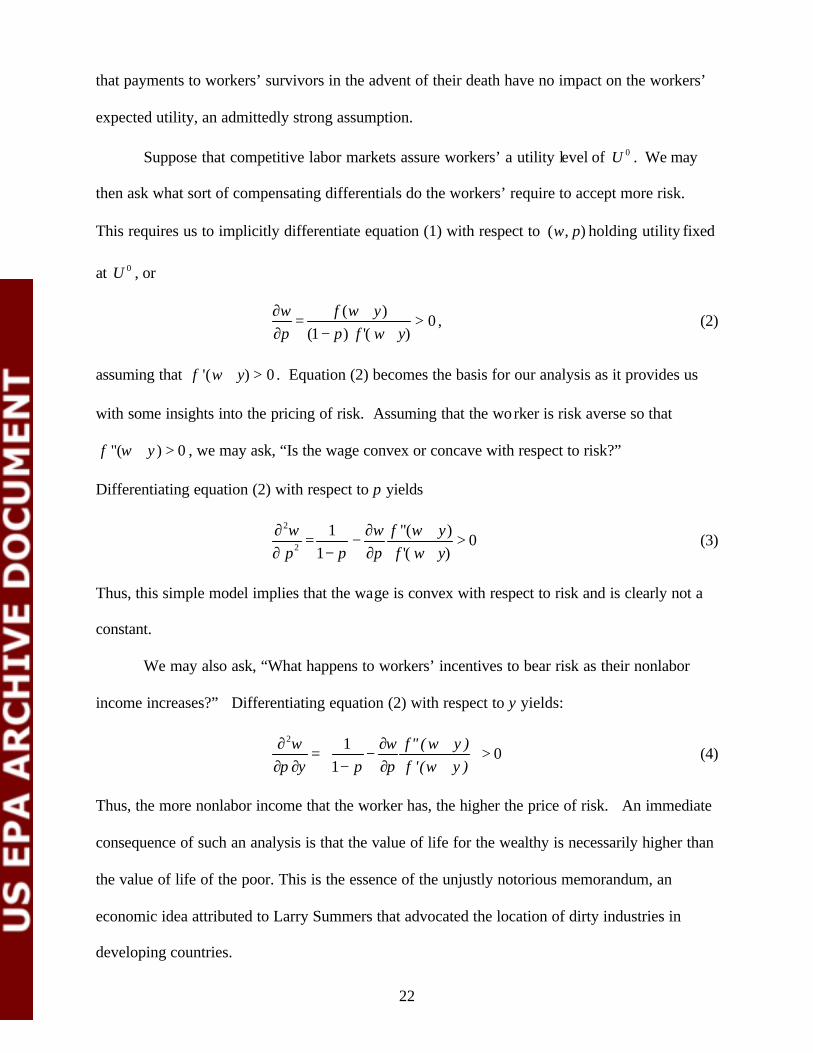
We may also ask, “What happens to workers’ incentives to bear risk as their nonlabor

income increases?” Differentiating equation (2) with respect to y yields:

2 10

1w w f " ( w y )

p y p p f '(w y ) ∂ ∂ +

= − > ∂ ∂ − ∂ + (4)

Thus, the more nonlabor income that the worker has, the higher the price of risk. An immediate

consequence of such an analysis is that the value of life for the wealthy is necessarily higher than

the value of life of the poor. This is the essence of the unjustly notorious memorandum, an

economic idea attributed to Larry Summers that advocated the location of dirty industries in

developing countries.

23

The result in equation (4) also indicates that any attribute that increases worker wealth

also increases their risk price. Thus, workers with greater education, or with college majors that

are financially more lucrative, should demand higher prices for accepting risk. Similarly,

workers who earn less in the labor market - women, blacks, Hispanics, and other minority groups

- should, according to the theory, have a lower price of risk.

These comparative statics summarize the guidance that the theory of compensating

differentials offers the applied researcher: the wage should increase with increases in job risk,

the rate of increase in the wage for an increase in risk is in itself increasing in risk, and wealthier

workers should require a greater compensation to take on risk. This is not a particularly great

deal of guidance for the applied researcher: the specified wage function for estimation should be

convex in job risk and the price of risk should be increasing in worker wealth. Yet, even this

guidance is not robust. If we make slight alteration to the model, such as relaxing the

assumption that the workers do not value payments to their survivors, even these modest

restrictions prove difficult to retain.

As is often the case, however, the theory does provide a critique of the existing empirical

work. While applied researchers have generally assumed that the wage-risk relationship is log-

linear, nothing in the theory suggest such a simple relationship. Thus, we expect that the price of

risk is a relatively complex function of worker characteristics and wealth.

III. Some Problems The fundamental approach in the hedonic literature is to use variation in the risk of various jobs

to assess the payment necessary to assume additional risk on the job. All the identification of the

price of risk necessarily depends on the assignment of occupation, industry, and location. This

fundamental feature of the hedonic wage literature is at once its greatest strength – it allow the

researcher to get informed estimates of the risk that workers face – and the source of several

problems in the identification of the price of risk.

24

To make the discussion concrete, let us begin with a standard wage equation used in the

hedonic wage literature. Assume that the wage equation is of the form:

*i i i iln(w ) X rβ γ ε= + + (5)

where iln(w ) is the natural logarithm of the ith worker’s wage, *ir is the measure of risk

(potentially a vector), iX is a vector of covariates that the researcher knows affects the wage,

( , )β γ are coefficients to be estimated, and iε is the error term of the regression. This form of

the wage equation is what Viscusi (1993) calls the “basic approach in the literature” and admits a

natural interpretation for γ as the “price of risk.”

Much of the advances in applied microeconomics over the last thirty years have arisen

from suspicion about parameter estimates from equations similar to equation (5). Researchers

have wondered whether *i i( X ,r ) are measured with error, whether *

i i( X ,r ) is uncorrelated with

the unobservables in that determine wage, which are captured in the error term, iε , and whether

the functional form of equation (5) is appropriate.

If one could think of a thought experiment to identify the willingness of workers to pay

for risk reductions, it would probably go something like this. A researcher could offer workers

otherwise identical jobs to their current jobs, but jobs that had less risk (the likewise informative

experiment of offering job with higher risk would probably fail to get the IRB approval from the

researcher’s institution).

In contrast, researchers are forced to use variation that is the result of workers optimal

choices rather than the random assignment of risk. Thus, one suspects that risk and the

unobservables, iε , may lead to substantially biased estimates. Moreover, despite the lack of

theoretical guidance, researchers often begin by assuming a specification of a wage function like

equation (5). One wonders if the arbitrary specification of the price of risk as a log- linear affects

25

the magnitude of the estimates of the price of risk as well. In what follows, we explore these

issues in greater detail.

a. The impact of errors in variables on the estimated price of risk The starting point for our analysis is a wage equation of the form:

*i i i iln(w ) X rβ γ ε= + + . (5)

For purposes of this discussion, we assume that 0i iCov(X , )ε = and 0*i iCov(r , )ε = (so that the

risk measures and other covariates are exogenous). To keep the discussion simple, we assume

that *ir is a scalar.

If the researcher could measure *i i( X ,r )perfectly, Ordinary Least Squares (OLS)

estimation of equation (5) would provide consistent and efficient estimates of the parameters

( , )β γ . Unfortunately, there are numerous reasons to suggest that the measure of job risk ( *ir ) is

mismeasured and perhaps mismeasured badly. First, government fatality reports are inherently

an inaccurate estimate of job risk: they are realizations of a random variable. For instance,

suppose there are kN workers in the kth industry (or occupation) category, and each of these

workers are subjected to a risk, *kr . Unfortunately for the researcher, the government’s tally of

deaths in the kth category is not exactly equal to the expected number of deaths, *k kr N . Rather,

the government’s tally is equal to the random variable kD . Using the random variable kD , the

researcher constructs an estimate of *kr as k k kr D / N= . While *

k kE(r ) r= , it is almost certain

that *k kr r≠ . Thus, let *

k k kr r η= + , where kη is the measurement error associated with the

variable kr .

The actual situation is much more complicated. Industry and occupation are very poorly

measured, even in carefully collected data sets such as the PSID and CPS. For instance, using a

CPS supplement that interviewed both the employee and employer, Mellow and Sider (1983)

26

document that employers and employees agree on three-digit industry codes only 84.1 percent of

the time. Even for the broader one-digit industry codes, the rate of agreement is only 92.3

percent. The situation for occupation codes is even worse. Employee and employer agree only

57.6 percent of the time about the three-digit code and only 81.0 percent of the time for one-digit

codes. Thus, there is a substantial degree of measurement error in the industry and occupation

measures. Mellow and Sider document that for the sample in which both firm and worker agree

on three-digit industry code, the estimated price of risk for non-fatal accidents is 50 percent

higher than the sample as a whole. Leigh (1987), however, argues that the impact of this

measurement error on fatality risk is much smaller.

Even when workers correctly identify their industry and occupation it is still likely that

the measurement of job risk is in error. Past studies have indicated that job risk differs by firm

size, region, and worker characteristics. Thus, when we make the further substitution for the ith

worker’s risk (who is in the kth industry/occupation class) that *i kr r= , we are undoubtedly

introducing measurement error. Thus, let

*k i ikr r ν= + (6)

where ikν represents the measurement error associated with using kr as a proxy for *ir .

The measurement error undoubtedly attenuates the estimates of the coefficient γ . Indeed

Hausman, Newey, and Powell (1991) term this the “iron law of econometrics.” From an

empirical standpoint the relevant question is, “How severe is attenuation bias that results from

the measurement error ikν ?” Instrumental Variables (IV) estimation can answer that question.

The usual problem with IV estimation is finding appropriate instruments for the

mismeasured variable. Fortunately, because both the BLS and NIOSH data provide estimates of

job risk, there is no shortage of instruments. To see why, suppose that we estimate equation (5)

using the BLS three-digit occupation measure of fatality risk to assign the worker’s job risk.

27

Given the disagreements in three-digit occupation codes that Mellow and Sider (1983)

document, there will probably be considerable measurement error in the variable. The NIOSH

job risk measures, using one-digit industry and state variation, can be used as instruments for the

BLS measures. While both measures probably contain a great deal of measurement error, both

should be highly correlated with the worker’s actual risk level.

Griliches (1986) outlines assumptions about the form of the measurement error necessary

to insure that instrumental variables will produce consistent estimate of ( , )β γ . Let us illustrate

this point with a simple example. In column (1) of Table 1, we present OLS estimates of the

price of risk using the 1995 CPS and the Bureau of Labor Statistics (BLS) estimates of fatality

risk from their Survey of Working Conditions and the National Institute of Occupational Safety.

The dependent variable is the logarithm of the workers average wage from the previous year.

Covariates include a quartic in age, a set of dummy variables measuring the respondents’

education, and dummy variables indicating whether respondents are African American, Asian,

Hispanic, or other race. The variable of interest is the industry fatality rate. We estimate

separate regressions for men and women. One could certainly add several additional covariates

(firm size, marital status, union membership to name but a few), but the specification of the

equation is sufficiently rich to illustrate our point. The OLS estimates for men indicate a

statistically significant and economically meaningful price of risk. The implied value of a

statistical life for a one in 100,000 reduction in the risk of a job related fatality is about $2.9

million for men when evaluated at the mean wage. For women, the relationship is not

statistically significant, but the point estimate of the price of risk remains economically

substantial. The implied value of a statistical life for a one in 100,000 reduction in the risk of a

job related fatality is about $1.4 million for women when evaluated at the mean wage.

Our discussion above, however, suggests that one might think these estimates are

attenuated by the measurement error in the BLS measure of risk. To illustrate the magnitude of

28

the potential attenuation bias, we implement a simple Instrumental Variables (IV) estimator of

the price of risk. If we let k,tr be the BLS measure of industry- level fatality risk, we use 1k,tr + as

an instrument for current job risk. This IV estimator will remove the random fluctuations that

result from the fact that k,tr is a random variable. It does not correct for possible

misclassification of industry, which would also attenuate the coefficient estimates, because we

continue to use the respondents’ reported industry to assign fatality risk.

We report the results in column (2) of Table 1. For men, the IV point estimate is 3.7

times the size of the OLS point estimates, suggesting a value of a statistical life of about $10.6

million. For women, the results are even more dramatic. The IV point estimate is 5.6 times the

size of the OLS point estimate, and the value of statistical life increases to $7.7 million. Indeed,

we cannot reject the hypothesis that the point estimate for men and women are the same.

These estimates are meant to be merely illustrative. As we noted above, there is

undoubtedly much remaining measurement error in our measure of job risk because we continue

to rely on respondents’ reported industry to assign job risk. In addition, these estimates, as well

as many of the other estimates in the literature, may suffer from the other problems we address in

this paper. These IV estimates, however, do indicate that the reliance of OLS to estimate the

price of risk may substantially understate the price of risk.1

B. Correlation of risk and other job attributes A second problem that arises when attempting to measure the impact of job risk on wages is the

possible correlations of job risk and other attributes. In principle, collecting information about

the characteristics of jobs could solve this problem. This has generally been the approach of

estimating hedonic price functions in the housing market. For occupations, however, this would

appear to be a hopelessly complex task. Jobs differ by whether they require the worker to travel, 1 Black, Berger, and Scott (2000) demonstrate that if the measurement error is mean reverting that IV estimation may overstate the magnitude of the relevant parameter. As they demonstrate, anytime the variable of interest contains a lower bound, such as zero, the measurement error may be mean reverting.

29

to work nights, to work outdoors, to work under stress, to perform tasks repetitively, or to work

with disagreeable colleagues or customers. Jobs also differ in whether they offer health benefits,

vacations, flex time, pensions, and opportunities for advancement. In addition, jobs impose

different human capital requirements on workers, with some requiring workers to acquire

complex skills while others require relatively little of workers.

Such variation would present no intrinsic problem if it were uncorrelated with job risk.

Unfortunately, such variation is probably highly correlated with job risk. For instance, the

ability to operate a chainsaw is probably a requirement for many a logging job. It is also a major

reason why such jobs are dangerous. Similarly, underground coal mining places the working in

a dirty environment, deep under the surface of the earth. While these are two of the more

obvious examples, one suspects job risk is highly correlated with other undesirable

characteristics of the job.

C. Correlation of risk and unobserved worker productivity At least since Brown (1980), economists have recognized that the nonrandom sorting of workers

into job risk may cause substantially biased estimates of the price of risk. It is closely related to

the problems caused by correlation of job risk and unobserved job characteristics. Both the

correlation of risk and unobserved worker productivity and the correlation of risk and other job

attributes pose problems because they induce a correlation of job risk and the error term in the

regression equation (5).

Brown’s approach is to modify equation (5) slightly:

*it it it i itln(w ) X r uβ γ α= + + + (7)

where the subscript t indexes time while the subscript i continues to index the individual. 2 As

Brown had panel data, he was able to estimate the fixed-effect model given in equation (7). The

estimation of the fixed-effect model requires that the data be demeaned so that the dependent

2 Duncan and Hulmlund (1983) pursue a similar identification strategy.

30

variables becomes it iln(w ) ln(w )− (where iln(w ) is the mean of the logarithm of wages for the

ith person) and the independent variables become it iX X− and * *it ir r− . As the data are

demeaned, individuals who do not change jobs (and hence do not change risk classification) do

not make any contribution to the variation used to identify γ .

The fixed-effect model also sweeps out all time invariant characteristics of the individual,

including those not observed by the researcher. It allows these time invariant characteristics,

captured by the iα term, to be correlated with either itX or *itr and still produce consistent

estimates of the parameters ( , )β γ . While this is clearly a less restrictive assumption than

required for the OLS estimation of equation (x), the fixed-effect model suffers from two

potentially important disadvantages. First, as Griliches and Hausman (1986) and Bound and

Krueger (1991) note, the use of fixed-effect models exacerbates any measurement error

problems. As we noted above, there are strong reasons to believe the data on job risks contain

substantial measurement error so this problem may be severe.

A second potential problem with the use of fixed-effect models relies necessarily on the

changes in job risk faced by individuals, presumably resulting from changes in jobs. The

assumption of the fixed-effect model is that this variation is uncorrelated with unobservables that

determine wages. Yet, if time- invariant unobserved characteristics might be correlated with job

risk so might time varying unobserved characteristics, and it is not obvious which correlation

might be larger.

Given the common structure of the correlation of risk and unobserved worker

productivity and the correlation of risk and other job attributes, it is not surprising that solutions

to both problems have a common structure. What is necessary is to find sources of exogenous

changes in job risk. Thus, as in the case of measurement error, an instrumental variables

approach would appear to be in order.

31

Unfortunately, these problems appear to be much more unremitting problem than the

problem of measurement error. While one might look for natural experiments in which changes

say in government safety regulations or technology changes occur, it is difficult to conceive of

experiments that would allow us to measure the price of risk in a wide number of settings.

Indeed, there are technological advances that have had large impacts on workplace safety (e.g.,

the introduction of long-wall coal mining), but these technological advances also affect the

demand for labor and the skill mix of labor in the industry or occupation. This makes it

extremely difficult to distinguish the impact of demand changes on wages from the impact of

reduction in risk on wages. Hence, technological advances do not appear to be legitimate natural

experiments. Hence, one might wish to focus on changes in government policy that reduced job

risk.

Professor William Evans of the University of Maryland suggested to us one of the most

promising natural experiments. In 2000, transportation accidents accounted for 43.5 percent of

the over 5,900 occupational fatalities. As Professor Evans correctly notes there is tremendous

heterogeneity in accident rates by states. For instance, for each mile driven, drivers are 3.2 times

more likely to die in Mississippi than in Massachusetts. One could use variation within states

across time to examine how changes in job safety that arise from improved vehicle safety and

improved enforcement of drunk driving laws have affected wages.

We believe this to be a very clever approach to estimating the price of risk. It has the

particular advantage of not greatly changing other characteristics of the job. Yet, it identifies

only modest changes in risk. While transportation fatalities account for about 44 percent of job

related deaths, this is due to the prevalence of driving on the job rather than the driving being

particularly dangerous. Indeed, only about 6.3 percent of fatal motor vehicle accidents occurred

while on the job. Thus, driving on the job appears to be relatively safe.

32

The nature of the variation induced by the instrument is therefore at relatively low levels

of risk and affects primarily those who drive on the job.3 If one takes the specification of

equation (5) seriously so that the re is one, and only one, price of job risk, then this experiment

identifies that price. In the next section, however, we discuss reasons why we might expect the

price of risk to vary.

D. Is there a single price to estimate? Again, consider the standard hedonic wage equation

*i i i iln(w ) X rβ γ ε= + + . (5)

The equation makes three strong assumptions that may do violence to the data. First, it assumes

that the researcher knows the appropriate vector of covariates *i i( X ,r ) . Second, it assumes the

coefficients ( , )β γ are constants, rather than functions or random vectors. Thus, the impact of

risk on wages is the same for a 45-year-old black female accountant as for a 27-year-old white

male high school graduate working in the oil fields of Texas. Third, it assumes a log- linear

relationship between the wage and the covariates. As Angrist and Krueger (1999) emphasize,

the use of OLS estimation may provide very misleading estimates if these assumptions are

incorrect.

There are several reasons to believe that this may not be true. As Hwang, Reed, and

Hubbard (1992) and Evans and Viscusi (1993) emphasize, differences in the productivity of

workers or the wealth of consumers may induce differences in the demand for safety. If safety is

a normal good, then wealthier workers will prefer less dangerous jobs than their poorer

counterparts. Thus, in equilibrium, we should see poorer workers demanding higher risk jobs,

and the price of risk then becomes a function of the wealth of the worker as the theory in Section

3 Some individuals are killed when struck by a motor vehicle when not driving another motor vehicle.

33

II predicts. Yet, little of the existing empirical work accounts for the heterogeneity in the price

of risk that the theory implies.

Of course, there are many other reasons to believe that the price of risk is not constant.

Workers differ in their attitude toward risk, their life expectancy, their ability to avoid accidents,

and other attributes. Similarly, the theory outlined above implies a convex relationship between

wages and risk, but the theory does not imply a log linear relationship between the price of risk

and wages.

Existing evidence suggests considerable heterogeneity in the parameter estimates and

equation specification. For instance, in the appendix to their 1988 paper, Moore and Viscusi

estimate a Box-Cox transformation that rejects both the log-linear and the linear-linear

specification. Nor do estimated prices for risk appear to be constant. Leigh (1987) finds

evidence that samples of men and women produce much different prices of risk. Viscusi (1981)

reports substantial variation in estimates of the value of life by quartiles of the distribution of job

risk. For instance, the implied value of life for workers in the first quartile of fatality risk is $5

million while the implied value for workers in the fourth quartile is only $2.8 million.

In the remainder of the subsection, we outline an empirical strategy for implementing

nonparametric estimates of the price of risk that will minimize the impact of assumptions about

functional form on the estimates. Our strategy requires that our risk measures be discrete. Thus,

suppose we divide jobs into K risk categories (for deciles, 10K = ). Let the wage of the ith

worker in the jth risk category, ijY , be given by

1 2ij j i ijY g ( X ) j , ,...Kε= + = (8)

where iX is a vector of characteristics that determines earnings and ijε is again the error term.

The function jg ( )⋅ is an unknown function that determines wages. We may define the price of

risk,

34

ijk i ij ikp ( X ) Y Y= − , (9)

which is the cost per hour of moving the ith worker from the jth risk class to the kth risk class.

The fundamental problem is that we observe either ijY or ikY but never observe both. We

propose to estimate the “missing” wage using nonparametric methods. For low dimensions of

the iX vector, the estimation is simply the mean wage of all individuals in the appropriate risk

class who have identical characteristics to the jth worker (e.g., all black men who are 27 years

old with a high school degree in the kth risk class). We call these the cell-matching estimators.

This is precisely the strategy of Heckman and Vytlacil (2001).

For higher dimensions of the iX vector, the cell-matching estimator is infeasible because

of the limited number of matches. A commonly used alternative is the propensity score

matching estimator of Rosenbaum and Rubins (1983); see Heckman, Ichimura, and Todd (1997,

1998) and Smith and Todd (2000) for a discussion of propensity score estimates and examples of

their use. Until recently, propensity score matching has been limited to cases in which the

variable of interest was binary. For case job risk, this would require the division of jobs into a

risky and safe classification, a much too restrictive formulation in my view. Fortunately, Imbens

(1999) and Lechner (2000) have shown that propensity score matching extends to finite numbers

of alternatives. Thus, we can use propensity score matching to estimate the “missing” wages.

Once the missing wages are estimated, the price of risk is just

ijk i ij ikˆp ( X ) Y Y= − (10)

where ikY is the estimated missing wage. Given these individual prices of risk, the average price

of risk for moving from the jth to the kth risk category may be calculated as

1

jN

ijk ii

jkj

p ( X )p

N==∑

(11)

35

The nonparametric estimation of the price of risk avoids making any assumptions about the

functional form of the jg ( )⋅ and allows the price of risk to vary across individuals. Hence, we

could calculate the price of risk for, say, college-educated Hispanic women between the ages of

30 and 34. The nonparametric estimation also imposes no functional form restriction as we

move across the various risk classes. Thus, moving from the first to the second decile of risk

may have a different price than moving from the fourth to the fifth decile.

A possible objection to this nonparametric approach is that it forces the risk measures to

be discrete. We can employ an alternative estimation strategy that allows for the risk measure to

be continuous but it does so at a cost of requiring a parsimonious specification of the covariates,

iX . Let iX be of sufficiently low dimension that we may again employ the cell-matching

estimator. We may for the kth cell consider the estimation of the equation

*ik k k ik ikY h ( r )α ε= + + (12)

where ikY is the ith worker’s wage, kα is a constant to be estimated, and ikε is the regression

error. The function *k ikh ( r ) is a cell-specific function that measures the price of risk. While the

precise functional form is unknown, under weak assumptions we can approximate the function

using a spline function, a Taylor series approximation, or a Fourier series expansion. Because

these approximations are linear in the parameters, the functions *k ikh ( r ) may be aggregated

across groups of workers or across all workers. We can then compare the results of the

semiparametric estimation to both the nonparametric estimation outlined in this section and the

parametric estimation of equation (5).

E. The support problem A major feature of the nonparametric approach outlined above is that the researcher’s inference

is limited by the support of the data. In parametric models, the support of the data is

considerably less transparent because the estimated function allows for inference in areas outside

36

the support of the data. The validity of these inferences, however, is questionable. Heckman,

Ichimura, Todd (1997, 1998), Heckman, Ichimura, Smith, and Todd (1998), and Heckman,

Smith, and Clements (1997) demonstrate how differences in the support of the distributions of

covariates may lead to incorrect inference in parametric models.

For the purposes of the EPA, the range of the risk measure is extremely important. As

we demonstrated above, the price of risk is an increasing function of the risk level. Given that

environmental risk may have a much wider range than job risk, it is important for the EPA to be

cognizant of the limited range of risk for which labor market data may be used to identify the

value of reducing risk.

As Kniesner and Leeth (2000) emphasize, the range over which workers face risk is

extremely small. For instance, in 1997 the probability of dying in a work-related accident was 5

in 100,000. In contrast, an individual is twice as likely to die in a home accident (10 in 100,000),

and over three times as likely to die in an automobile accident (16 in 100,000). NIOSH (1993)

documents that between 1980 and 1989, the traumatic fatality rate had substantial variation

across one-digit industries, ranging from a low of 1.37 per 100,000 workers in real estate,

insurance, and finance to a high of 31.91 in mining. Thus, working in mining results in a

probability of a traumatic fatality that is about as twice as high as that for motor vehicle

accidents. If we focus on a particular industry in a particular state, however, the rates can be

much higher. For instance, for mining in Kentucky (primarily underground coal mining) the

average death rate is 63.4 workers per 100,000.

Even this variation may be overstated for particular demographic groups. Kentucky coal

miners tend to have limited education. To illustrate how heterogeneous is the variation in job

risk, in Table 2 we present the distribution of occupational risk (using the NIOSH data) for

individuals with a high school degree and individuals with a bachelor’s degree. We separate the

samples by gender as well.

37

Clearly, college educated men and women use a part of their increased wealth to

purchase safer jobs. For both men and women, college educated people have much safer jobs

than those with a high school degree. Yet, the theory of hedonic implies that the price of risk

varies by the respondents’ wealth and the level of risk they face, and respondents with more

education are clearly wealthier than their less educated counterparts. When assessing the value

of a statistical life for the college educated, data on job risk has a much smaller range than data

from the high school graduates. Thus, inference from labor market data for college graduates is

valid over a smaller range than for high school graduates.

Similarly, women, regardless of their education level, sort into jobs that are safer than

men. Thus, when assessing the value of a statistical life for women, data from the labor market

provides intrinsically less information for women than for men.

IV. Conclusions In this paper, we explore several problems in the estimation of the price of risk and outline some

strategies to circumvent these problems. We note that existing data on job risk necessarily

contains a great deal of measurement error. Fortunately, the data are sufficiently rich to allow us

to implement instruments for this measurement error. Our preliminary estimates suggest that

current estimates of the price of risk may well be substantially understated because of the

inherent measurement error in job risk measures.

We outline how recent advances in nonparametric estimation may be used to estimate the

price of risk nonparametrically. The use of nonparametric estimation allows the researcher to

make inference about the price of risk without having to make strong distributional assumptions

on the unobservables or functional form assumptions on the conditional mean function. It has

the added advantage of requiring the researcher to confront the limited range for which labor

market data may be used to infer what consumers are willing to pay to reduce fatality risk.

38

References Angrist, Joshua D. and Alan B. Krueger. 1999. “Empirical Strategies in Labor Economics.” In

O. Ashenfelter and D. Card (eds.), Handbook of Labor Economics, Volume 3A. Amsterdam: North Holland.

Black, Dan A., Mark C. Berger, and Frank A. Scott. 2000 “Bounding Parameter Estimates with

Nonclassical Measurement Error.” Journal of the American Statistical Association September 95(3): 739-48.

Bound, John and Alan B. Krueger, 1991. “The Extent of Measurement Error in Longitudinal

Earnings Data: Do Two Wrongs Make a Right?” Journal of Labor Economics 9(1) (January): 1-24.

Brown, Charles. 1980. “Equalizing Differences in the Labor Market.” Quarterly Journal of

Economics 94(1) (February): 113-34. Duncan, Greg J. and Bertril Holmlund, 1983. “Was Adam Smith Right after All?” Journal of

Labor Economics 1(4) (October): 366-79. Evans, William N., and W. Kip Viscusi. 1993. “Income Effects and the Value of Health.”

Journal of Human Resources (Summer): 728-47. Garen, John E. 1988. “Compensating Wage Differentials and the Endogeneity of Job

Riskiness.” Review of Economics and Statistics 70(1) (February): 9-16. Griliches, Zvi. 1986. “Economic Data Issues,” In Zvi Griliches and Michael D. Intriligator

(eds.), Handbook of Econometrics, Volume 3. Amsterdam: North Holland. Griliches, Zvi and Jerry A. Hausman. 1986. “Errors in Variables in Panel Data.”

Journal of Econometrics. 31:93-118. Hausman, Jerry A., Whitney K. Newey, Hidehiko Ichimura, and James L. Powell. 1991.

“Identification and Measurement Polynomial Errors- in-Variables Models.” Journal of Econometrics 50(3) (December): 273-95.

Heckman, James J., Hidehiko Ichimura, Jeffrey A. Smith, and Petra Todd. 1998.

“Characterizing Substitution Bias Using Experimental Data.” Econometrica 66(5) (September): 1017-98.

Heckman, James J., Hidehiko Ichimura and Petra E. Todd. 1998. “Matching as an Econometric

Estimator.” Review of Economic Studies 65(2) (April) 261-94. Heckman, James J., Hidehiko Ichimura and Petra E. Todd. 1997. “Matching As An

Econometric Estimator: Evidence from Evaluating a Job Training Program.” Review of Economic Studies 64(4): 487-36.

39

Heckman, James J., Robert LaLonde, and Jeffrey Smith. 1999. “The Economics and Econometrics of Active Labor Market Policies.” In O. Ashenfelter and D. Card (eds.), Handbook of Labor Economics, Volume 3A. Amsterdam: North Holland.

Heckman, James J. and Richard Robb, Jr. 1985. “Alternative Methods for Evaluating the

Impact of Interventions.” In James J. Heckman and Burton Singer (eds.), Longitudinal Analysis of Labor Market Data. Cambridge: Cambridge University Press, pp.156-1245.

Heckman, James J., Jeffrey A. Smith, and Nancy Clements. 1997. “Making the Most Out Of

Programme Evaluations and Social Experiments: Accounting for Heterogeneity in Programme Impacts.” Review of Economic Studies 64(4) (October): 487-36.

Heckman, James J., and Edward Vytlacil. 2001. “Identifying the Role of Cognitive Ability in

Explaining the Level of Change in the Return to Schooling.” Review of Economics and Statistics 83(1) (February): 1-12.

Hwang, Hae-shin, W. Robert Reed, and Carlton Hubbard, 1992. “Compensating Wage

Differentials and Unobserved Productivity.” Journal of Political Economy 100(4): 835-858.

Imbens, Guido W. 1999. “The Role of the Propensity Score in Estimating Dose-Response

Functions.” NBER Technical Working Paper # 237. Cambridge, MA: National Bureau of Economic Research.

Kane, Thomas J., Cecilia E. Rouse, and Douglas Staiger. 1999. “Estimating Returns to

Schooling When Schooling is Misreported.” NBER Working Paper #7235. Cambridge, MA: National Bureau of Economic Research.

Kniesner, Thomas J. and John D. Leeth. 1991. “Compensating Wage Differentials for Fatal

Injury Risk in Australia, Japan, and the United States.” Journal of Risk and Uncertainty 4(1) (January): 75-90.

Kniesner, Thomas J. and John D. Leeth. 1995. Simulating Workplace Safety. Boston: Kluwer

Academic Publisher. Kniesner, Thomas J. and John D. Leeth. 2000. “Workplace Safety Policy: Past, Present, and

Future.” Center for Policy Research Policy Brief No. 19. Syracuse, NY: Syracuse University. http://www-cpr.maxwell.syr.edu/pbriefs/pblist.htm.

Lechner, Michael. 2000. “Identification and Estimation of Causal Effects of Multiple

Treatments under the Conditional Independence Assumption.” Unpublished paper. St. Gallen, Switzerland: University of St. Gallen. August.

Leigh, J. Paul. 1987. “Gender, Firm Size, Industry and Estimates of the Value of Life.” Journal

of Health Economics 6(3) (September): 255-73. Mellow, Wesley and Hal Sider. “Accuracy of Response in Labor Market Surveys: Evidence and

Implications.” Journal of Labor Economics 1(4): 331-44.

40

Moore, Michael J. and W. Kip Viscusi. 1988. “Doubling the Estimated Value of Life: Results Using New Occupational Fatality Data.” Journal of Policy Analysis and Management 7(3) (Spring): 476-90.

National Institute for Occupational Safety and Health. 1993. Fatal Injuries in the United States,

1980-1989: A Decade of Surveillance. NIOSH Publication #93-108. Washington, DC: U.S. Department of Health and Human Services, Center for Disease Control.

Rosenbaum, Paul and Donald Rubins. 1983. “The Central Role of the Propensity Score in

Observational Studies for Causal Effects.” Biometrika 70(1) (April): 41-55. Smith, Jeffrey and Petra Todd. 2000. “Does Matching Overcome LaLonde’s Critique of Non-

experimental Estimators.” Unpublished paper. London, Ontario: University of Western Ontario. November.

Viscusi, W. Kip. 1978. “Labor Market Valuations of Life and Limb: Empirical Estimates and

Policy Implications.” Public Policy 26(3) (Summer): 359-86. Viscusi, W. Kip. 1979. Employment Hazards: An Investigation of Market Performance.

Cambridge, MA: Harvard University Press. Viscusi, W. Kip. 1981. “Occupational Safety and Health Regulation: Its Impact and Policy

Alternatives.” In J. Crecine (ed.), Research in Public Policy Analysis and Management, Volume 2. Greenwich, CT: JAI Press, pp. 281-99.

Viscusi, W. Kip. 1993. “The Value of Risks to Life and Health.” Journal of Economic

Literature 31(5) (December): 1912-46.

41

Table 1: Impact of Measurement Error on the Price of Risk,

1995 CPS and BLS Fatality Data

OLS

Estimates (1)

IV Estimates

(2)

Industry death rate per 100 workers – men

0.916 (2.09)

3.40 (4.94)

Implied value of statistical life at mean wage and 2,000 hours

$2,854,000 $10,606,000

Industry death rate per 100 workers – women

0.576 (1.10)

3.24 (3.04)

Implied value of statistical life at mean wage and 2,000 hours

$1,370,000 $7,717,000

Notes: The dependent variable is the natural log of the worker’s wage. The independent

variables include a quartic in the worker’s age, a vector of dummy variables that control for the

worker’s education, and dummy variables indicating whether the worker is Hispanic, Asian,

African American, or other race. The instrument for the IV estimates is the industry death rate

from 1995. There are 21,368 observations in the men’s regressions and 20,472 in the women’s

regressions. Workers are aged 25 to 60, inclusive. T-statistics given in parentheses.

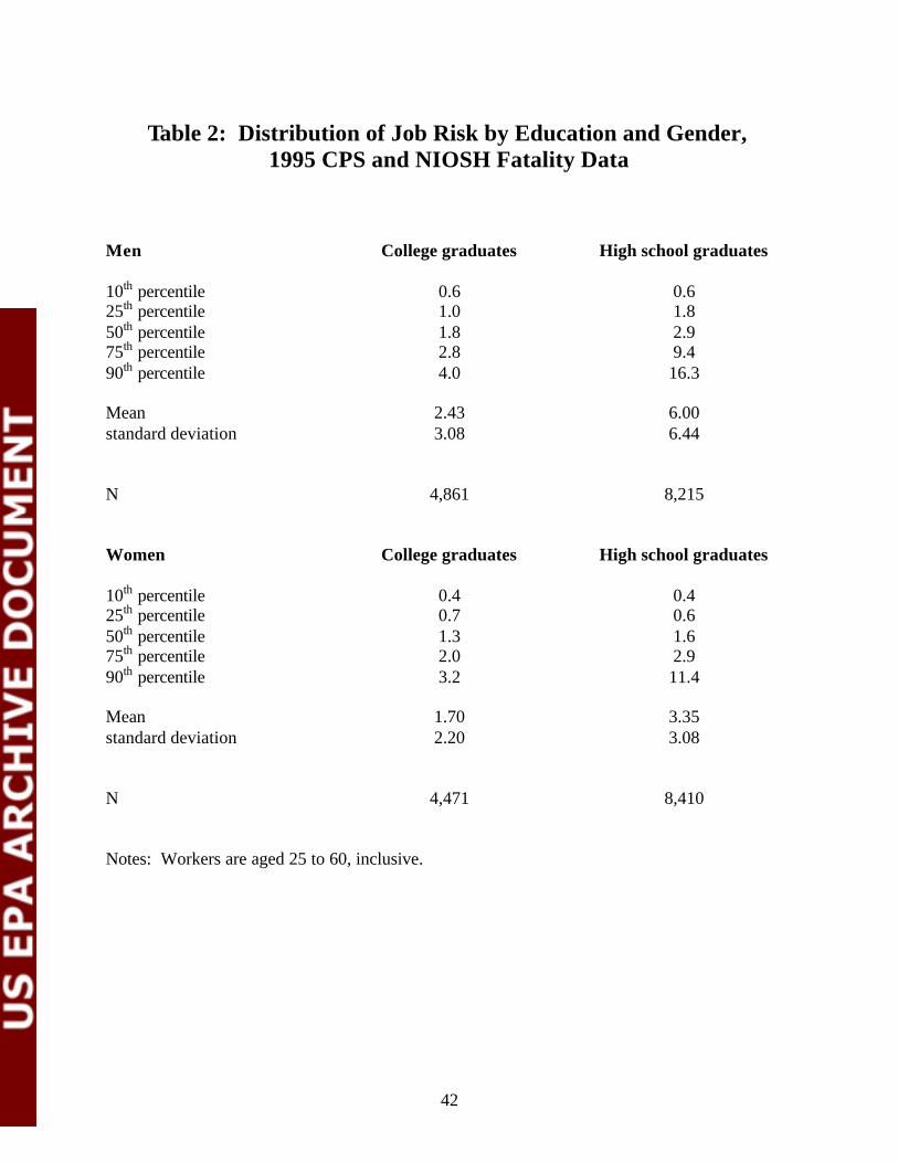
42

Table 2: Distribution of Job Risk by Education and Gender, 1995 CPS and NIOSH Fatality Data

Men College graduates High school graduates

10th percentile 0.6 0.6 25th percentile 1.0 1.8 50th percentile 1.8 2.9 75th percentile 2.8 9.4 90th percentile

4.0 16.3

Mean 2.43 6.00 standard deviation

3.08 6.44

N 4,861 8,215 Women College graduates High school graduates

10th percentile 0.4 0.4 25th percentile 0.7 0.6 50th percentile 1.3 1.6 75th percentile 2.0 2.9 90th percentile

3.2 11.4

Mean 1.70 3.35 standard deviation

2.20 3.08

N 4,471 8,410 Notes: Workers are aged 25 to 60, inclusive.

43

Data Appendix:

There are two major sources of government-reported job risk: the Bureau of Labor Statistics

(BLS) estimates from their Survey of Working Conditions and the National Institute of

Occupational Safety and Health (NIOSH) estimates from their National Traumatic Occupational

Fatality Survey. The NIOSH data provide one-digit occupation (or industry) mortality rates by

state, while the BLS data contain three-digit occupation codes but do not provide any regional

variation.

Our data on workers is from the March 1995 Supplement of Current Population Survey. The

1995 CPS provides data on 1994 earnings, occupation and industry. The CPS provides a

reasonably rich set of covariates for inclusion in wage equations. The data set is a random

sample of the US population.

44

Willingness to Pay for Mortality Risk Reductions: The Robustness of VSL Figures from Contingent Valuation Studies

--Working Paper*--

PRESENTED BY: ANNA ALBERINI

UNIVERSITY OF MARYLAND COLLEGE PARK, MD 20742


45

WILLINGNESS TO PAY FOR MORTALITY RISK REDUCTIONS:

THE ROBUSTNESS OF VSL FIGURES FROM CONTINGENT VALUATION STUDIES

By

Anna Alberini Department of Agricultural and Resource Economics

University of Maryland College Park, MD 20742

December 10, 2001

Paper presented at the Workshop

“Economic Valuation of Mortality Risk Reductions: Assessing the State of the Art for Policy Applications,” Silver Spring, MD, 6 November 2001

1. Introduction Reductions in risk of death are arguably the most important benefit underlying many health, safety, and environmental legislative mandates. For example, in two recent analyses of the benefits of U.S. air quality legislation, The Benefits and Cost of the Clean Air Act, 1970-1990 (US EPA, 1997) and The Benefits and Cost of the Clean Air Act, 1990-2010 (US EPA, 1999), over 80 percent of monetized benefits were attributed to reductions in premature mortality. In quantifying the benefits of policies that save lives, Viscusi (1993) recommends a range of Values of a Statistical Life (VSLs) from $3 to 7 million (1990 dollars) based on a review of labor market and other studies. The majority of these studies are compensating wage studies using observed workplace risk- income tradeoffs to infer the VSL. Only five of the twenty-six studies are contingent valuation (or conjoint choice) surveys directly eliciting willingness to pay for a specified risk reduction (Gerking et al., 1999; Jones-Lee et al., 1985, Viscusi et al., 1991b, Miller and Guria, 1991). Contingent valuation is a valuation technique that directly asks individuals to report information on their willingness to pay for an improvement in environmental quality, health or safety, or in the provision of a public good. This technique can and has been applied to both public and private goods. A change in the risk of death experienced by an individual, for example, is a public good if the risk reduction is delivered by a public program, such as an environmental or transportation safety program, but a private good is the risk reduction is delivered by an action or product (e.g., carbon monoxide detector) privately purchased and used by an individual. In conjoint choice surveys, respondents are asked to state which they prefer between two commodities (or policy packages)

46

described by a set of attributes. One of the attributes is usually the price of the good, or the cost of providing a government program. Because they are based on what individuals state they would do under specified, but hypothetical, circumstances, both contingent valuation and conjoint choice are examples of stated-preference methods for obtaining WTP for a commodity. In contingent valuation surveys, changes in small probabilities have proven to be a very difficult commodity to value. Respondents must be explained probabilities and risks concepts in the first place. They may find it difficult to grasp that many risks can be avoided or reduced, but at a cost. Moreover, the risk changes to be valued are usually very small, and likely to be dismissed as meaningless by the respondents. It is, then, not surprising that many recent CV surveys about reductions in mortality risks result in numerous zero WTP responses, and that the WTP amount announced by respondents fail to increase with the size of the risk reduction as predicted by economic theory (Hammitt and Graham, 1999). Statistical modeling of the WTP responses is further complicated by the fact that the underlying distribution of WTP has long, and hard-to-nail-down, tails, and that respondents with positive WTP must be distinguished from those respondents who hold no value at all for the risk reduction. This raises concerns about the robustness of these studies’ estimates of mean and median WTP, and relationships between WTP and individual characteristics such as income, age, education, and health status of the respondent. These relationship are used to test the internal validity of these studies and to test the internal validity of the responses, and can potentially be used for benefit transfer purposes. The purpose of this research is three-fold. First, I will request the original data collected through the five stated preferences studies and will re-analyze them to check the quality of the data and examine the robustness of the econometric estimates of VSL with respect to a variety of criteria (described below). In other words, I will try to find out if alternative analyses and statistical models of the WTP data would have resulted in largely different estimates of WTP/VSL. Second, I will search the recent literature, looking for articles in peer-reviewed economics journals and for unpublished discussion papers eliciting WTP for reductions in the risk of death. I will carefully examine the survey materials, the questionnaires used, the risk reduction scenarios presented to the respondents, the wording and the nature of the payment questions, and the sample of respondents, comparing them to those used in the three contingent valuation studies mentioned above. Third, for some of these papers or articles—those where the program delivering the risk reduction, the population surveyed, and the quality of the study itself suggest that results could be applicable to environmental policy and other health and safety situations—I will obtain the original datasets from the authors and econometrically re-analyze the WTP responses to assess the robustness of the estimates of WTP/VSL.

47

It should be emphasized that I do not wish to perform a meta-analysis of the VSL figures produced by stated preference studies. The purpose of this research is to examine the studies one by one, and not to uncover the across-study relationship between WTP and characteristics of the study design, the populations being surveyed, and the risk reductions being valued. In the remainder of this paper, I describe possible criteria to assess the econometric robustness of the estimates of WTP and VSL.

II. Possible Robustness Criteria A. Data Quality Checks My first order of business is to examine whether the responses from a contingent valuation survey eliciting WTP for mortality risk reduction satisfy basic requirements suggested by economic theory. When the CV survey is conducted using the dichotomous-choice format,4 for example, the percentage of “yes” responses to the payment question should decline with the bid amount. Figure 1 reports the percentage of “yes” responses to the payment question observed in a survey of US residents, where two independent subsamples of respondents were asked to report information about their WTP for risk reductions of different size. The figure shows that the percentage of “yes” responses declines regularly with the bid amount, ranging from 73% at the lowest bid amount ($70) to 35% at the highest bid amount ($725) for a risk reduction of 5 in 1000. It is also important to check that the bid amounts assigned to the respondents in the survey cover a reasonable portion of the range of possible WTP values. Alberini (1995a, 1995b) shows that when the distribution of WTP is assumed to be symmetric and the statistic of interest is mean/median WTP, placing of the bids on one side of the median and/or too far away from the center of the distribution may result in a significant loss of efficiency of the estimates of mean/median WTP.

4 In a dichotomous-choice contingent valuation survey, respondents are asked to state whether or not they would purchase the good to be valued, or vote in favor or against of a proposed government program, if the cost to their household was $X. If the respondent is in favor of the program, or says he would buy the good, then his WTP exceeds $X. If the respondent declines to buy the good, or votes against the program, then WTP must be less that the dollar amount X. The dollar amount, $X, is generally termed the bid value, and is varied across respondents. Binary response econometric models are then fit to the responses to this payment question, and estimates of mean or median WTP are usually obtained exploiting the properties of the distribution WTP is assumed to follow (see, for instance, Cameron and James, 1987).

48

In most applied work, WTP is assumed to follow an asymmetric distribution, such as the log normal or the Weibull. In my own research, I have found that failure to present respondents with bid amounts nicely spread over the possible range of WTP values can seriously impair the researcher’s ability to obtain stable estimates of the parameters of the distribution. In Figure 1, for example, the percentage of “yes” responses to the payment questions for the 1 in 1000 risk reductions is consistently less than 50%, implying that the researcher can only trace out the upper tail of the distribution of WTP. To illustrate the consequences of skewed bid designs, I conducted Monte Carlo simulations where the responses to the dichotomous choice payment questions are assumed to be driven by draws from a log normal distribution. The bid amounts are regularly spaced and range from the 5th to the 95th percentile of the distribution of WTP. I generate artificial dichotomous choice responses to the payment questions, fit a probit model where the binary response is regressed on a constant and on log bid, and estimate mean and median WTP. The sample size is 1000 and the procedure is repeated for 1000 replications. The experiment is then repeated with only the five largest bids, and the four largest bids, and for a log normal distribution with a larger variance. Descriptive statistics of the distribution of the resulting estimates of WTP are shown in Figures 2 and 3. When the variance of WTP is relatively small, mean and median WTP are relatively stable even if the bids cover a limited portion of range of WTP values. When the variance of WTP is large, however, mean WTP is estimated with a bias (ranging from 18 to 53%), and the bias is more severe when the bid design misses portions of the range of WTP. Similar considerations hold for the standard errors of the estimates of mean WTP. This shows that an unbalanced design has the potential for leading to biased and grossly inefficient estimates of WTP, and that this problem appears to be more severe when the distribution of WTP has a large variance. These findings confirm that it is important to check if existing CV studies have used balanced bid designs. A preliminary examination of recent articles and papers suggests that even well received, influential studies may have suffered from a poor choice of bid values: Johannesson and Johansson (1996), for instance, report that that the percentage of respondents willing to pay the lowest bid level in their survey (100 SEK) is 53%, while the percentage of respondents willing to pay the highest bid level is 4%—a rather unbalanced bid design. B. Choice of distribution for WTP. In their report of a contingent valuation surveys eliciting non-use values for Prince William Sound in Alaska, Carson et al. (1995) show that the estimates of both mean and median WTP from dichotomous choice CV survey data can be very sensitive to the distributional assumption about WTP. This suggests that alternative distributions should be attempted with the data from existing CV surveys. It is also important that researcher move away from fitting logit or

49

probit models to the responses to dichotomous choice payment questions, as these models imply that WTP is allowed to be negative. C. Discrete Mixtures. While it is routinely assumed that respondents will answer “yes” to a dichotomous choice payment question if their WTP amount is greater than the bid, and “no” when their WTP amount is greater than the bid, it seems possible that the sample might be “contaminated” with some responses that do not abide by the economic paradigm. Examples of such contaminating responses include “yea-saying,” “nay-saying,” and completely random responses. Yea-saying implies that the respondent answers “yes” with probability 1, regardless of the bid amount. By contrast, nay-saying implies that the respondent answers “no” with probability 1, regardless of the bid amount. When the responses are completely random, the respondent answers “yes” with probability 0.5, and “no” with probability 0.5, regardless of the bid value. Yea-saying behavior is possible, for example, when the respondent wishes to please the interviewer, or hopes that by answering in the affirmative to the payment question the survey will be terminated soon. Nay-saying behavior, on the other hand, might be observed when the respondent dislikes government programs, even though he might privately attach a value to the good or environmental quality improvement provided by the program. It is also possible that respondents exhibit nay-saying behaviors when they are opposed to new taxes, and/or when they fear to commit to something that they do not fully understand. Finally, completely random responses might be due to complete confusion about the scenario, failure to understand the commodity being valued, no interest in the survey, and/or poorly written questions or survey materials. (Completely random responses might also result from a data entry error, in which case, however, the problem arises for reasons other than the respondent’s behavior.) Because CV studies eliciting WTP for mortality risk reduction must present respondents with probabilities, which are difficult for most people to comprehend, response effects like the ones described above seem plausible. While it is possible, in some cases, to identify yea-sayers, nay-sayers and completely random responses by making judicious use of debriefing questions and interviewer observation, in most cases with dichotomous choice payment questions we do not know whether the response to the payment question is legitimate or is due to one of these contaminating behaviors. From the statistical point of view, the presence of contaminating responses can be addressed by specifying a (discrete) mixture of distributions. Assume for the sake of simplicity that the observed sample responses come from a mixture of two distributions. Let the first component of the mixture be a well-behaved distribution of WTP with cdf F(•), while the second component of the mixture is yea-saying behavior. Let α be the

50

probability of (fraction of the sample that engages in) yea-saying behavior, while (1-α) is the probability (fraction of the sample) of announced responses that are consistent with true WTP amounts. When a “yes” response is observed, then the contribution to the likelihood is (1) αθααα +−⋅−=⋅+>⋅−= ));(1()1(1)Pr()1()Pr( iiii BFBWTPyes where B is the bid amount, while the contribution to the likelihood by an observed “no” response is: (2) );()1()Pr()1()Pr( θαα iiii BFBWTPno ⋅−=≤⋅−= . Equations (1) and (2) are, therefore, different from the typical contributions to the likelihood in statistical models of dichotomous choice responses, the difference arising from having to account for the fact that an observed “yes” has a probability (1-α) of being a genuine “yes” and α of being the result of yea-saying behavior. When yea-saying exists and is not adequately accounted for, the estimated survival curve of WTP (i.e., 1 minus the cdf of WTP, which traces out the percentage of respondents willing to pay any given bid amount) lies above the true survival curve (see Figure 4). This will lead to overestimating both mean and median WTP. Similarly, if the second of the two discrete components of the mixture was “nay-saying,” the appropriate contributions to the likelihood would be: (3) ));(1()1()Pr()1()Pr( θαα iiii BFBWTPyes −⋅−=>⋅−= , and (4) αθααα +⋅−=⋅+≤⋅−= );()1(1)Pr()1()Pr( iiii BFBWTPno . The estimated survival function of WTP will, therefore, lie below the true curve, which will result in underestimating mean and median WTP. Finally, in the presence of completely random responses, the contributions to the likelihood are: (5) αθααα 5.0));(1()1(5.0)Pr()1()Pr( +−⋅−=⋅+>⋅−= iiii BFBWTPyes (6) αθααα 5.0);()1(5.0)Pr()1()Pr( +⋅−=⋅+≤⋅−= iiii BFBWTPno . The estimated survival curve will be below the true curve for bid amounts lower than the median, will cross the true curve at the median (since the probability of a “yes” is 0.5 for both legitimate responses and random responses) and will be above it for bid amounts greater than median WTP (see Figure 5).

51

The mixing probability α must be estimated by the method of maximum likelihood. It is also possible to make α a function of covariates, such as gender, age, education and attitudinal variables. As α is a probability, the logit or probit link is appropriate:

)( βα ixΦ= . In on-going research, I am exploring how important the shape of the distribution of WTP and the size of α are in determining the maximum likelihood routine’s ability to identify α (Alberini and Carson, 2001). Guided by the results of that research, I hope to fit discrete mixtures to the data from CV surveys about mortality risk reductions to assess the influence of contaminating responses. D. Zero WTP Especially when the mortality risk reductions being valued are small, many people report that they are not willing to pay anything at all to obtain the risk reduction. In earlier analyses, zero WTP responses have been pooled with non-zero WTP responses and continuous or interval-data versions of the tobit models have been fit to the data (Kriström, 1997; Krupnick et al., forthcoming). This approach, however, assumes that the relationship between the regressors and WTP is the same for both respondents with positive WTP amounts and respondents with zero WTP. If this assumption is incorrect, the estimates of WTP and the regression coefficients in the WTP functions might be biased. To avoid such biases, the sample might be interpreted as a mixture of two populations: the first component of the mixture is a degenerate distribution of WTP (all WTP values being equal to zero), while the second component of the mixture is a well-behaved random variable. Specifically,

(7)

−=

)1(yprobabilitwith);(~yprobabilitwith0

αθα

wtpfWTP

where f denotes the probability density function of WTP and is indexed by a vector of parameters θ. Equation (7) might be applied, for example, to the data from the Gerking et al study. Its regression analyses assume a tobit model with double truncation to account for the presence of numerous zero WTP responses, and for the fact that the highest value shown to the respondents in the payment card was $6000. Mean and median WTP estimated from such a mixture might be compared with mean and median WTP from the tobit model. E. Endogenous Regressors

52

Contingent valuation studies eliciting WTP for mortality risk reductions have sometimes asked respondents to evaluate their own baseline mortality risks (Gerking et al., 1988) and/or the risk reductions attainable if certain measures are taken or policies are passed (Persson et al., 2001). WTP is then regressed on baseline risk and/or the risk reduction thus measured. However, it is possible that both WTP and the self-assessed level of risk (or risk reduction) share common unobservable individual characteristics, resulting in their endogeneity with one another. Coefficient estimates based on OLS or ML that assume risk to be exogenous will, therefore, be biased, resulting in incorrect inference about marginal WTP and about the relationship between WTP and baseline risk. To address this problem, it is necessary to specify an additional equation relating respondent-assessed baseline risks to respondent characteristics and other factors, and to estimate two systems of simultaneous equations, one for self-assessed risks and one for WTP. It would be interesting to see how the regressions presented in Gerking et al. (1988) and Persson et al. (2001) might change if the simultaneity of risk and WTP is explicitly allowed for. In the Gerking et al study, for instance, respondents were to place their own occupation on a risk ladder, and to subsequently report their WTP (WTA) for reducing (increasing) risk by one notch. It would seem appropriate to model both perceived risk and WTP as a function of individual socioeconomic variables, risk aversion and attitudes, and to allow for common, unobserved factors to influence both perceived risk and WTP. In Persson et al. (2001), respondents are asked to value a reduction in the risk of being killed in a transportation accident. The baseline risk is assessed by the respondent, after he or she is told what the average risk for a person of their age and gender is. The risk change in expressed as a percentage (10, 50, or 99 percent) of the baseline risk. WTP is regressed on baseline risk, risk change, and other individual characteristics, but both baseline risks and risk changes are likely to be endogenous with WTP. Johannesson et al. (1991) survey patients contacted at a health care center in Sweden, asking them to assess their subjective risks of death due to hypertension as well as their subjective risk reduction associated with a medical intervention. The risk reduction was not found to be a statistically significant predictor of WTP, a result perhaps due to the fact that the risk reduction is endogenous with WTP. Similar concerns about endogeneity might hold for the data collected in the Viscusi et al. study. In this study, the authors implement a form of conjoint analysis, engaging respondents in tradeoffs between chronic diseases with a specified risk of death (a nerve disease, and two forms of lymphoma with different severity), the risk of death in an automobile accidents, and dollars. The tradeoffs were elicited by asking respondents to indicate which city they would choose between two, each city having a specified level of

53

risk and a specified cost of living. The survey was self-administered and computerized, and allowed the research to change the attribute levels of the cities until indifference was reached. The researchers also ask questions intended to capture respondent risk aversion and attitudes towards risk, and find that risk aversion correlates well with the WTP responses and with the tradeoffs between risks of different type. Here, it would seem plausible that the answer to the risk aversion questions and the WTP/risk tradeoff questions share common, unobservable characteristics, and that they should be treated as econometrically endogenous. F. Outliers Outliers may be defined as observations such that WTP is disproportionately large (or small) for the level of the regressors associated with that observations. In dichotomous-choice CV studies, WTP is not directly observed, suggesting that the formal definition of an outlier might be modified to denote an observation such that a “yes” response to the payment question was observed when the probability of “yes” is very low, or a “no” response was observed when the probability of a “no” is very low (Copas, 1988). To identify outliers and assess their impact on the estimates of mean and median WTP, one might consider excluding from the sample respondents whose implied WTP values exceed specified fractions of their income (e.g., 5%, 10% or 25% percent) and examining how the estimates of mean and median WTP change. It is also possible to identify outliers using the jackknife, a statistical technique whereby the model is re-estimated n times, after excluding the j-th respondent from the sample, while retaining all others, for j=1, 2, …, n. This results in a vector of n estimates of mean and median WTP, the goal of the researcher being that of identifying which particular observations appear to be responsible for large changes in mean or median WTP. To my knowledge, relatively little attention has been dedicated to outliers in mortality risk CV studies. An exception is Lanoie et al. (1995). These authors find that when three influential observations are excluded from the sample, the VSL estimated from the CV component of their study drops from $22-27 million to $15 million (1995 Can. Dollars). G. Sample Selection Bias. If a mortality risk survey tends to recruit respondents among those persons with unusually high (or low) interest in abating mortality risk, the estimates of WTP may be affected by sample selection bias. To correct for sample selection bias, it is necessary to specify and estimate two econometric equations. The first is a probit participation equation, which predicts the probability of participating in the survey as a function of individual characteristics. Let P* denote propensity to participate,

54

(8) iiP ηγ += z* with z a vector of individual characteristics, γ a vector of coefficients, and η a normally distributed error term with mean zero and variance equal to one. Let P be a binary indicator that takes on a value of 1, denoting participation in the survey, if P* is greater than zero. The second equation explains WTP as a function of a vector of individual characteristics x: (9) iiWTP εβ += x* , where η and ε are correlated, their covariance being equal to σ. Because WTP is observed only for those persons who participated in the survey, one estimates

(10) error)()(

0| * +Φ

+=>γγφ

σβi

iiPWTP

zz

x .

In practice, this system of equations is estimated in two stages. The first stage is a probit predicting the probability of participating in the survey. The estimated coefficients are used to build the Mills’ ratio term )ˆ(/)ˆ( γγφ ii zz Φ included in the WTP equation. It is clear that to estimate the probit model it is necessary to have information about the survey participants, as well as information about those persons who were sent questionnaires or otherwise solicited to participate in the survey, but declined to. With mail surveys, Cameron et al. (1999) suggest saving the addresses and zipcodes of all individuals who were sent questionnaires and imputing to those persons who do not return the completed questionnaire the characteristics (such as median income, percentage of college educated adults, percent of home ownership, etc. from the Census) of the residents of his or her zipcode. This procedure assumes that an individual is much like his or her neighbors. With phone surveys, it might be possible to ask some questions of the person who answers the telephone, and to obtain some information about him or her, even if he or she elects not to continue the survey. Once the two-stage estimation procedure is completed, mean WTP is estimated (assuming normally distributed WTP) as βx . Notice that the estimate of β is biased unless one explicitly includes the correction term )ˆ(/)ˆ( γγφ ii zz Φ in the WTP equation. To illustrate, Gerking et al’s study used a mail survey to elicit information about WTP and WTA for changes in occupational risks. The survey questionnaires were mailed to a random sample of 3000 US residents, and to an additional sample of 3000 respondents, randomly selected among the residents of 105 US counties with disproportionately large concentrations of high-risk industries. The ages, income, education levels, and other characteristics of those who elected to fill out and return the questionnaires can therefore be compared with those of the US population, using Census and Current Population

55

Survey data. If the researchers kept track of the addresses of the mail questionnaires who did not return the questionnaire, it is possible to check, using multivariate probit regressions, whether participation in the survey is more likely in areas—such as Census tracts, zipcodes or counties—where the residents have certain characteristics. H. Alternative econometric models. In the Gerking et al study, the WTP responses are treated as if they were on a continuous scale, although the correct interpretation of the responses is that an individual’s WTP falls between the amount he or she picked on the payment card and the next highest amount. Re-specifying and re-estimating the likelihood function accordingly (Cameron and Huppert, 1988) could result in different estimates of mean WTP, and in different regression coefficients. III. Conclusions. WTP Responses from surveys valuing mortality risks need to be carefully inspected and care must be taken when modeling them and obtaining WTP/VSL estimates for use in policy. In this paper, I have proposed a variety of criteria that could be used to assess the quality of the data and fit alternative models of WTP. The goal of the research is to apply these criteria and to assess the econometric robustness of estimates of VSL ava ilable in the literature.

56

References Anna Alberini (1995a), “Optimal Designs for Discrete Choice Contingent Valuation Surveys: Single-bound, Double-bound and Bivariate Models,” Journal of Environmental Economics and Management, 28, 187-306. Anna Alberini (1995b) “Efficiency v. Bias of Willingness-to-Pay Estimates: Bivariate and Interval Data Models,” Journal of Environmental Economics and Management, 29, 169-180. Alberini, Anna, and Richard T. Carson (2001), “Yea-Sayers, Nay-sayers, Or Just Plain Confused? Mixtures of Populations in Contingent Valuation Survey Responses,” presented at annual meeting of the European Association of Environmental and Resource Economists, Southampton, England, June 2001. Carson, Richard T., W. Michael Hanemann, Raymond J. Kopp, Stanley Presser, and Paul A. Ruud (1995), “Contingent Valuation and Lost Passive Use: Damages from the Exxon Valdez,” University of California San Diego Discussion Paper 95-02, January. Cameron, Trudy A. and Daniel D. Huppert (1989), “OLS Versus ML Estimation of Non-Market Resource Values with Payment Card Interval Data,” Journal of Environmental Economics and Management, 17, 230-246. Cameron, Trudy A., and Michelle D. James (1987), “Efficient Estimation Methods for ‘Closed-Ended’ Contingent Valuation Surveys,” Review of Economics and Statistics, 69(2), 269-276. Cameron, Trudy Ann, W. Douglass Shaw, and Shannon Ragland (1999), “Non-response bias in mail survey data: Salience v. Endogenous Survey Complexity,” in Joseph A. Herriges and Catherine L. Kling (eds.), Valuing the Environment Using Recreation Demand Models, Cheltenham, UK: Edward Elgar Publishing. Copas, J. B. (1988), “Binary Regression Models for Contaminated Data,” Journal of the Royal Statistical Society, Series B, 50(2), 225-265. Gerking, Shelby, M. De Haan and William Schulze (1988), “The Marginal Value of Job Safety: A Contingent Valuation Study,” Journal of Risk and Uncertainty 1(2): 185-200. Hammitt, James K. and John D. Graham (1999). “Willingness to Pay for Health Protection: Inadequate Sensitivity to Probability?” Journal of Risk and Uncertainty, 8, 33-62. Jones-Lee, M.W., M. Hammerton and P. R. Phillips (1985). “The Value of Safety: Results of a National Sample Survey,” Economic Journal, 95, 49-72.

57

Johannesson, Magnus and Per-Olov Johansson (1996), “To Be or Not to Be, That is the Question: An Empirical Study of the WTP for an Increased Life Expectancy at an Advanced Age,” Journal of Risk and Uncertainty, 13, 163-174. Johannesson, Magnus, Bengt Jonsson, and Lars Borquist (1991), “Willingness to Pay for Antihypertensive Therapy—Results for a Swedish Pilot Study,” Journal of Health Economics, 10, 461-474. Kriström, Bengt (1997), “Spike Models in Contingent Valuation,” Americal Journal of Agricultural Economics, 79(3), 1013-23. Krupnick, Alan, Anna Alberini, Maureen Cropper, Nathalie Simon, Bernie O’Brien, Ron Goeree, and Martin Heintzelman (forthcoming), “Age, Health, and the Willingness to Pay for Mortality Risk Reductions: A Contingent Valuation Survey of Ontario Residents,” Journal of Risk and Uncertainty. Lanoie, Paul, Carmen Pedro, and Robert Latour (1995), “The Value of a Statistical Life: A Comparison of Two Approaches,” Journal of Risk and Uncertainty, 10, 235-257. Miller, T.R. and J. Guria (1991), The Value of Statistical Life in New Zealand, Wellington, NZ: Land Transport Division, New Zealand Ministry of Transport. Persson, Ulf, Anna Norinder, Krister Halte, Katarina Gralen (2001), “The Value of a Statistical Life in Transport: Findings from a New Contingent Valuation Study in Sweden,” Journal of Risk and Uncertainty, 23(2), 121-134. Viscusi, W. Kip (1993), “The Value of Risks to Life and Health,” Journal of Economic Literature, XXXI, 1912-1943. Viscusi, W. Kip, Wesley A. Magat and Joel Huber (1991), “Issues in Valuing Health Risks: Applications of Contingent Valuation and Conjoint Measurement to Nerve Diseases and Lymphoma,” Draft report to EPA, Office of Policy, Planning and Evaluation under Assistance Agreement CR# 815455-01-1 and 814388-02.

58

Figure 1.

70150

500725

1/1000 (wave 2)

5/1000 (wave 1)

72.86

35.1743.79

12.890

10

20

30

40

50

60

70

80

%

Initial Bid

Percentage of "Yes" Responses to Initial WTP Question--US Study

59

Figure 2.

0

20

40

60

80

100

120

140

Dollars

Full design Top 5 bids Top 4 bids

Effects of skewed bid designs on WTP (log normal distribution, low variance)

Median WTP Mean WTP

60

Figure 3.

0

2000

4000

6000

8000

10000

12000

Dollars

Full design Top 5 bids Top 4 bids

Effect of Skewed Bid Designs on WTP: Log normal distribution, higher variance

Mean WTP Std err Mean WTP

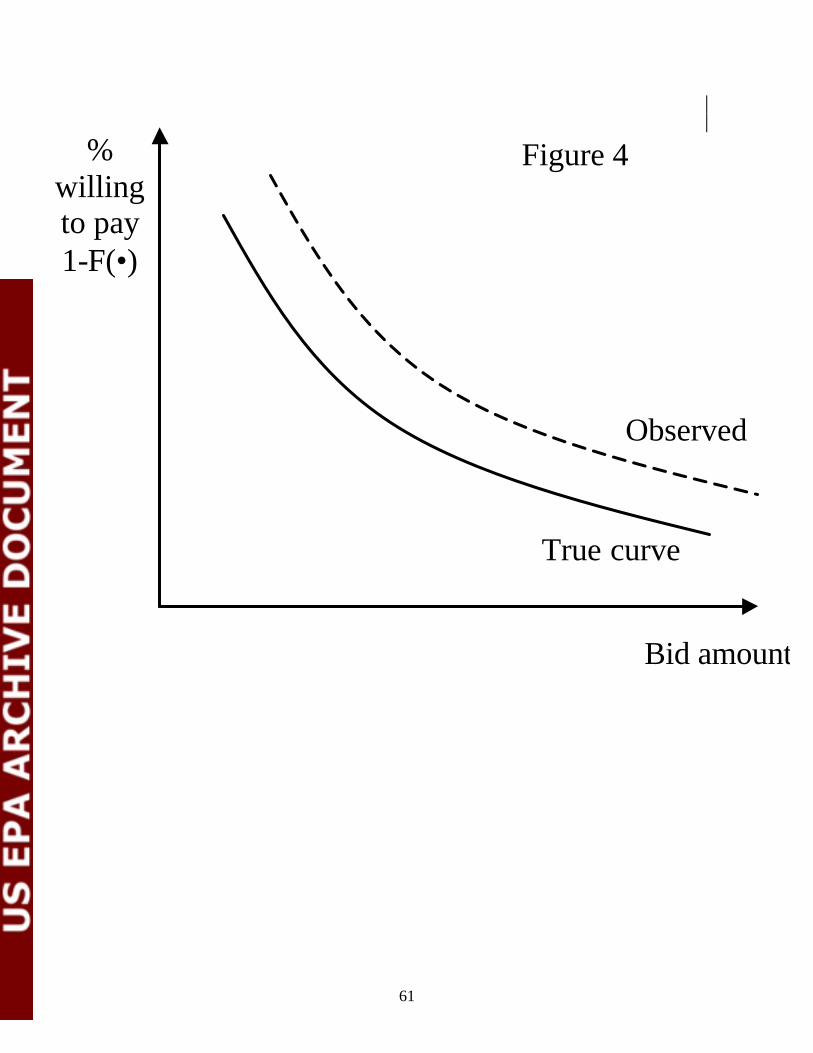
61

Observed

True curve

Bid amount

% willing to pay 1-F(•)

Figure 4

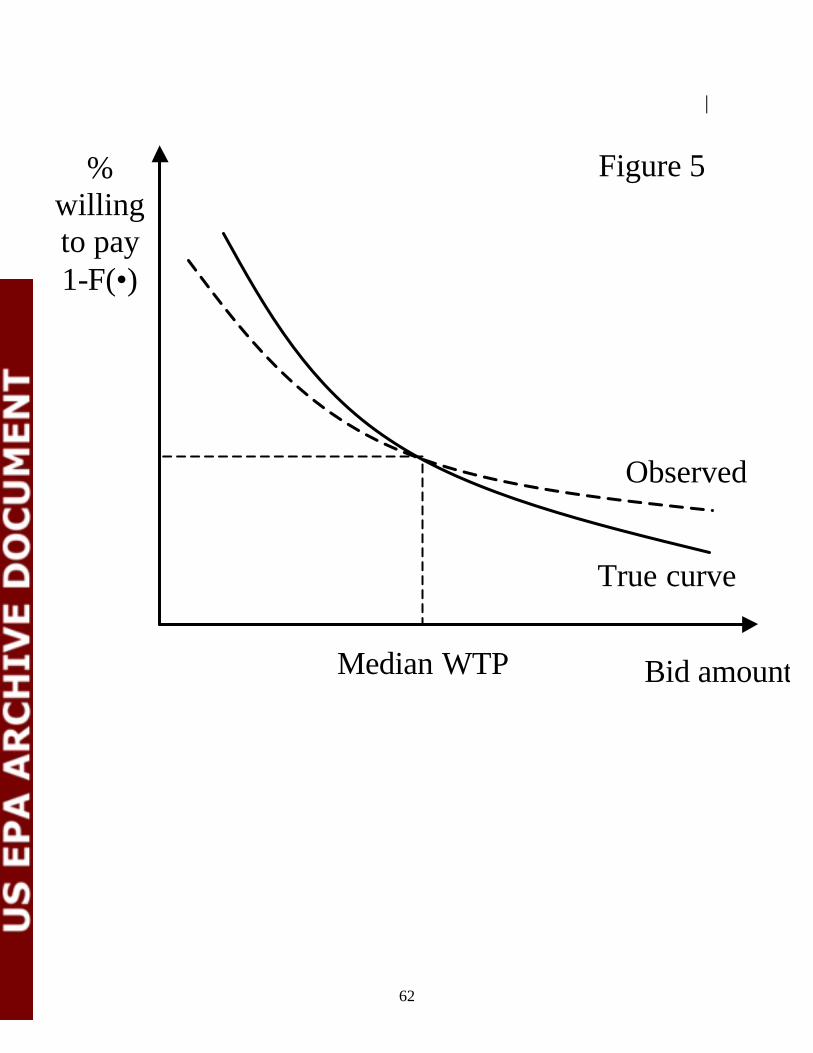
62

Observed

True curve

Bid amount

% willing to pay 1-F(•)

Median WTP

Figure 5

63

Self Protection and Averting Behavior, Values of Statistical Lives, and Benefit Cost Analysis of Environmental Policy

--Working Paper*--

PRESENTED BY: GLENN C. BLOMQUIST

UNIVERSITY OF KENTUCKY


“Self Protection and Averting Behavior, Values of Statistical Lives, and Benefit Cost Analysis of Environmental Policy”

Glenn C. Blomquist

Department of EconomicsUniversity of Kentucky

Lexington, KY 40506-0034and

Department of EconomicsStockholm School of Economics

Box 6501, Sveavägen 65SE-113 83 Stockholm Sweden

Phone: +46 8 736 92 84 Fax: +46 8 30 21 15 Email: [email protected](July 1, 2001 to June 30, 2002)

November 29, 2001

Prepared for “Economic Valuation of Mortality Risk Reduction: Assessing the State ofthe Art for Policy Applications,” an Environmental Policy and Economics Workshop held by theU.S. Environmental Protection Agency in Silver Spring, MD, on November 6-7, 2001. Comments of Bryan Hubbell, Ted Miller, Laura Taylor, and workshop participants areappreciated. I alone am responsible for the views in this paper.

2

Introduction.

Individuals can be observed in a variety of activities that affect their health and safety.

Protective behavior is evident in motorist choice of automobile type and use of safety equipment

such as seat belts. Choices concerning safety helmets, cigarette smoking and installation of fire

alarms change their risks of death. Choice of residence when housing markets encompass

Superfund sites influences the amount of risk they face. Visits to health clinics for preventive

care can reduce risks to health. The purpose of this paper is twofold. The first purpose is to

review studies which estimate values of mortality risks based on these tradeoffs which individual

consumers make. The common feature is that the estimates of values of small changes in

mortality risks are implied by observable consumer behavior as individuals protect themselves

against, or avert, risk. These values of mortality risks, for convenience, are sometimes referred

to as values of life or values of statistical life (VSL). Interest in estimates of these values exists,

in part, because the U.S. Environmental Protection Agency (EPA) evaluates policy that is

expected to have an impact on individuals’ health and safety and their mortality risks. Benefit

cost analysis (BCA) of such policy requires VSL estimates. The second purpose is to assess how

useful the estimates are for BCA of environmental policy and suggest directions for future

research.

This review is made with a constructively critical eye. While we economists find it

particularly easy to be critical, I think it is potentially too costly to go with our tendency in this

type of review because we risk fostering the notion that the whole methodology and entire body

3

1The ethical foundation for benefit cost analysis can be found in teleology. One form ofteleology is utilitarianism that judges goodness on the basis of choosing alternatives thatmaximize the good for all. A deontologist, in contrast, might object that any tradeoff of risk formoney or time is morally objectionable and the concept of VSL for use in BCA is wrong; seeBrandt-Rauf and Brandt-Rauf (1980).

of evidence on VSL are unreliable and, besides, the concept is immoral.1 A case can be made

that economists take for granted that we substantially agree that individual willingness to pay for

changes in risk is the best way to think about valuing the policy benefits and that sound,

theoretically based methods exist for estimating VSL. If we fail to emphasize what we know and

what we agree on while we strive to improve the practice of economics, we risk having the

whole approach dismissed as we are viewed as just squabbling, see The Economist (1997). A

great deal has been learned about valuing mortality risks since estimation of willingness to pay

for risk changes began nearly 30 years ago.

Frameworks for Estimating Values of Mortality Risks Based on Averting Behavior

The thought of inferring individuals’ values of reduction in mortality risks from their

behavior that is intended to influence that risk is appealing to economists. Situations in which

risk is at least partly a matter of choice provide opportunities to analyze behavior and estimate

the willingness to pay (WTP) for risk reductions or willingness to accept (WTA) compensation

for risk increments. These situations can involve choices among various types of work in the

labor market. These situations can involve choices in consumption, or household production,

activity. Self protection or averting behavior in consumption is the focus of this paper.

Smith’s (1991) “Household Production Functions and Environmental Benefit

Estimation” and Freeman’s (1993, Chapter 4) “Models for Indirect Benefit Estimation” provide

4

2 The model is only sketched here. For a more complete presentation see Blomquist(1979). For a more complete discussion of this approach including refinements, see Freeman(1993, Chapter 10).

broad reviews of the theory and use of household production approaches to valuing

environmental changes. Cropper and Freeman’s (1991) “Environmental Health Effects” and

Freeman’s (1993, Chapter 10) “Valuing Longevity and Health” provide careful reviews of

approaches to valuing changes in health risks, and in particular, to estimating values of changes

in mortality risks, VSLs. The literature is extensive and well developed and I will not attempt to

review in again in this paper. Instead, I will simply describe the two basic models that guide

thinking about valuing changes in mortality risks.

A basic model with the present and one future period captures the essence of estimating

risk tradeoffs in consumption.2 Let the individual maximize expected utility, E(U), that consists

of utility in the first period, U(C1,S) and expected utility in the second period, PU(C2), where U

is a well-behaved single period utility function, Ci is composite consumption in period i, i=1,2, P

is the probability of survival to period 2, and S preventive health or safety activity in which the

individual can engage. The production function for changing P is left general as P=P(S). P',

the marginal product of averting behavior, is the reduction in the mortality risk. P' is assumed to

be positive and diminishing. Averting activity can affect utility directly with US negative is S

generates disutility and positive if it generates utility. Maximization is subject to the budget

constraint, that the present value of expenditures on consumption and averting behavior, C1 + qS

+ d C2, cannot exceed the present value of income, wT + dwT + A, where q is the cost of

averting behavior, d is the factor that discounts the amount in period 2 back to the present, w is

the wage rate, T is time available for work in each period, and A is the present value of nonlabor

5

income. The cost of averting behavior, q, is composed of a money cost “m” and a time cost, awt,

where “a” is a factor which relates the value of time in averting activity to the wage rate and t is

the time input into averting activity.

The first order condition of interest is:

P'U(C2) / 8 = q - (US / 8) (1)

where 8 is the marginal utility of income. The left-hand side of equation 1 is the marginal

benefit of averting activity and the right-hand side is the marginal cost. The value of a gain in

the probability of survival (or reduction in mortality risk), is U(C2) / 8, which is the monetary

value of the utility of future consumption. Let this value be V so that V = U(C2) / 8. Notice that

if equation 1 is solved for V we have V = [q - (US / 8)] / P'. If for convenience of comparability

we evaluate V for a unit (0-1) change in P, then V is an estimate of VSL. So, the value of a

change in mortality risk for a unit change in P, VSL = [m + awt - (US / 8)] / P'.

Each component of the equation presents challenges in estimating VSL. The marginal

monetary cost, m, is sometimes negligible for averting activity. It is sometimes estimated by an

annual average cost. Marginal inputs of time, t, are sometimes small and sometimes substantial.

The value of time spent in producing changes in mortality risks can equal the market wage rate,

w, for the individual, or be some proportion of it, aw, as in motor vehicle travel. The monetary

worth of the marginal utility of the averting activity, US / 8, may be trivial, or may be a major

cost, such as has been the case with (nonpassive) seat belts in cars. Estimating P' may be simple

if expert estimates are available and individuals engaging in averting behavior perceive the

changes in risks to be the same as the experts. Any misperception of risk makes estimating the

perceived P' more challenging. I will discuss several of these components that are typically

6

3See Freeman (1993, Chapter 10) for a more complete presentation of life cycle models. The list of implications given above is based on his summary on page 334.

necessary for estimating VSL based on averting behavior. Despite the considerable effort that

has gone into estimating some components in many studies, I will recommend that more research

be done on some of the components in future research that is funded by EPA.

While a model with one future period is useful for understanding the basic tradeoff

between mortality risk and consumption, a multi-period model with uncertain lifetime allows

derivation of individual WTP for changes in mortality risks that would occur at different stages

of the life cycle. Life-cycle models can define, for example, the individual WTP now for a

change in the conditional probability of survival in 10 years. These models can be useful for

considering environmental policy that is expected to reduce future mortality risks. From life-

cycle models have followed several implications that have shaped expectations about VSL

estimates. Some testable implications are3: (1) generally WTP declines with age, (2) under

plausible conditions WTP exceeds discounted present value of future earnings, (3) WTP declines

with latency, and (4) WTP now for a risk reduction in year t is equal to WTP in year t for that

risk reduction discounted back to the present.

Current research continues to probe. For example, Shogren and Crocker (1991, 1999)

emphasize the importance of endongenous environmental risk and its implications for self

protection as a lower bound on the value of risk reductions. Bresnahan and Dickie (1995)

discuss the implications of endogenous risk and other issues in using values based on averting

behavior in policy evaluation. Shogren and Stamland (2001) show that the existence of

heterogenous workers with different unobservable skills to reduce their own mortality risks can

7

4Throughout this paper estimates are reported in 1998 U.S. dollars. The annual averageConsumer Price Index for all urban consumers for all items is used to convert values fromstudies with VSL reported in dollars for another year. The meta-analysis of VSL estimates fromthe labor market by Mrozek and Taylor (forthcoming 2002) reports VSL estimates in 1998dollars.

bias wage-risk estimates of VSL upward. Johansson (2001) using a life-cycle model to

demonstrate that, in contrast to the first implication listed above, there is no obvious age pattern

for WTP for mortality risk reductions over the life cycle. In this paper I will review estimates of

VSL based on self protection and averting behavior. I will comment on some of the issues in

using the basic model. I will note some of the results that are surprising given the implications

of life-cycle models, at least as we currently understand them.

Estimates of Values of Mortality Risks based on Self-Protection and Averting Behavior inConsumption

Interest in estimates of VSL has produced several reviews. Viscusi’s (1993) survey of

the literature included a summary of studies based on tradeoffs in consumption, or what he calls

outside of the labor market, see Table 1 (Viscusi, 1993, Table 5, p.1936.) It includes seven early

studies on highway speeds, seat belt use, smoke detectors, housing prices and air pollution, and

auto purchases. The average of the VSL estimates in 1998 dollars is $1.7.4 Miller (1990)

reviewed VSL estimates from all types of studies and based on 47 VSL estimates he considered

sound, he found an average VSL of $3.7 million in 1998 dollars. Using the previously reviewed

studies and 21 additional estimates, Miller (2000) reports his meta-analysis. Table 2 shows the

international studies included. They give an indication of the global interest in estimating VSL

and the values estimated for other countries, see Miller (2000, Table 1, p. 34.) Elvik’s (1995)

8

summary of averting behavior studies is shown in Table 3, see Elvik (1995, App. C, p. 19). One

feature of Elvik’s review is that he notes whether or not each study has a test of rationality, or

risk perception.

The most recent review, by de Blaeij et al. (2000), is a meta-analysis of all types of

studies that estimate VSL based on a tradeoff related to traffic safety. The summary from that

study is shown in Table 4, see de Blaeij et al. (2000, Table 1, p.31). The average VSL reported

in the paper is $5.0 million in 1998 U.S. dollars. It should be noted that 11 VSL estimates from

four different studies are included that are estimated from public policy decisions. While this

type of study reveals something about public decision making, the values are different in nature

from the values estimated from individual self protection, averting behavior. The public

tradeoffs tell us little, if anything, about individual WTP. Based on the values reported in their

Table 1, it appears that excluding the estimates based on public tradeoffs will increase the

average VSL because the values implied by public decisions tend to be lower. The increase is

not likely to be great given that there are 60 estimated values remaining and they do not appear

to be extremely different.

Table 5 shows my summary of eight relatively recent studies that estimate VSL based on

averting behavior in consumption. Hedonic analysis of prices of cars that have various fatality

risks, analysis of motorists’ use of safety equipment, analysis of bicyclists’ use of helmets,

analysis of highway speeds and fatalities, and hedonic analysis of prices of houses with various

cancer risks due to nearby Superfund sites are the methods used to estimate VSL. The range of

values for adults is something less than $2.6 million to $6.8 million. The average value for

adults is approximately $4.3 million in 1998 dollars if $2.0 million is used for the speed/fatality

9

study and averages are used for the two studies with a range reported. Four very recent studies

are worth more detail.

One recent study was presented by Ashenfelter and Greenstone (2001) at the symposium

in honor of Sherwin Rosen last May at the University of Chicago. They estimate the VSL from

changes in speeds on interstate highways. In 1987 federal law was changed to allow states to

raise the speed limit on rural interstates from 55mph to 65mph. Ashenfelter and Greenstone

analyze speeds and road fatalities for 28 states for which they can get data for the period 1982-

1993. Based on models which included state-by-road-type and year-by-road-type fixed effects,

they estimate that speeds increased by approximately 4% and fatalities increased by

approximately 36% in states which adopted the higher speed limit. They calculate the time

savings associated with the increase in speeds and it is approximately 221,000 hours. This

tradeoff between time gained and life lost implies an upper bound on VSL of approximately $2.6

million (1997 dollars) if time is valued at the wage rate. The estimate is an upper bound because

the tradeoff is observed only for states in which the ratio of time savings to VSL exceeds the

underlying VSL. Motorists would not have traded off the mortality risks if they had been worth

more than the savings in time. The second component of the paper is an effort to recover the

structural estimate of the VSL based on analysis of the tradeoff in each of the states. The

estimates of this “average” are lower than the upper bound estimate as expected, but they are

imprecisely estimated. Ashenfelter and Greenstone continue to work on this paper and their

estimates should be regarded as preliminary. However, their upper bound estimate appears to be

robust to many changes. One change in functional form that is not evidently sensible does

increase the estimate substantially and it is still being contemplated. If they use a value of time

10

5These estimates are based on laws being changed so that motorists can make tradeoffsfor time savings at the expense of bearing greater mortality risks. Motorists are assumed to basetheir behavior on the actual tradeoff of risks. This assumption is the same as in the labor marketin which workers are assumed to make the tradeoff between higher wages and the mortality risksthat actually occur. While one can question the assumption and attempt to obtain the subjectiveestimates of risk or adjust for perception bias, the tradeoff is no more ex post than the typicalestimate from self protection and averting behavior.

which is less than the wage rate, then their estimate will be reduced proportionately. Ghosh,

Lees, and Seal (1975) used observed speeds on British motorways to estimate VSL 26 years ago.

Although it is not as sophisticated as Ashenfelter and Greenstone’s, it is an early averting

behavior study which contributed to what is now considered something we know, that VSL is

greater than discounted foregone earnings5.

Gayer, Hamilton, and Viscusi (2000) analyze the housing market surrounding Superfund

sites in Grand Rapids, Michigan. They use a specially-constructed, expert measure of cancer

risk as well as distance measures and other proxies for physical risk. They find that the proxies

for risk can explain about half the variation in expert risk and that housing with less (either proxy

or expert statistical) risk sells for higher prices. After the release of the EPA Remedial

Investigation, premiums for safer locations imply values of statistical cancer of approximately

$4.1 - 4.8 million in 1998 dollars. If the share of the premium attributable to fatal risk and the

share of cancer cases that are fatal are the same, then this value is also an estimate of the VSL.

Estimates of VSL are much higher if prerelease risk perceptions are used. If the EPA is

interested in valuing reductions in cancer risks rather the VSL, then this study is especially

relevant to BCA.

Jenkins, Owens, and Wiggins (2001) calculate the VSL implied by use of bicycle helmets

and find it to be approximately $4.1 million in 1998 dollars for adults who purchase and wear the

11

helmets. They consider their estimate to be a lower bound because buyers and users find it

worth at least as much as the cost to gain the added protection. Including time and disutility

costs would increase the implied value and reinforce the claim that the estimate is a lower bound

if only money costs are relevant to the use decision. However, their estimated VSL is an upper

bound for bicyclists who are not buyers and users if time and disutility costs are zero. If

potential time and disutility costs are important for all bicyclists and those costs are different for

users and nonusers, then their estimate is not necessarily an upper bound for nonusers. It is not

clear what the VSL is for the average bicyclist. This aspect aside, their study is noteworthy in

that it is one of only a few that estimate VSL for children and the only published study that I

know of that infers a value from bicycle helmet use.

An ambitious hedonic study of prices of motor vehicles and associated fatality rates by

Mount, Weng, Schulze, and Chestnut (2001) seeks to estimate VSL for household members of

different ages. They build upon earlier related analysis and devote more attention to household

use of the vehicles and distribution within the household. A noteworthy characteristic of their

study is the set of detailed estimates of mortality risks that account for differences in vehicle use

by various members of households. Another advantage of their study is the inclusion of a wider

range of motor vehicles than passenger cars only and a rich set of driver characteristics. Their

preliminary estimates of VSL are among the highest of the recent studies. Their point estimate

of VSL for adults is $6.8 million in 1998 dollars.

One aspect of the recent estimates worth noting is that the simple average of the VSL

estimates for adults of $4.3 million is greater than the range of $1.5 - 2.5 million for estimates

from labor market studies in the meta-analysis by Mrozek and Taylor (forthcoming 2002).

12

Because I was under the impression that the labor market studies produced higher estimates, I

am surprised by this result and suggest that it bears more thought. Shogren and Stamland (2001)

offer a reason for upward bias in risk compensating wage studies. They demonstrate that if

workers differ in their individual, private ability to reduce risk and the ability is unobservable by

employers, then a market wage must be offered to attract the marginal worker who faces the

most risk of those employed. If the average risk of all workers is used to estimate a VSL, then it

is lower than that faced by the marginal worker and the VSL is biased upward. If unbiased

estimates from the labor market are even lower than the meta-analysis of Mrozek and Taylor

indicates, then more thought about the difference between them and the estimates from the recent

averting behavior studies is warranted.

Risk Perception and Values Implied by Averting Behavior in Consumption.

A crucial element in estimating VSLs from self protection and averting behavior is the

amount risk changes when the individual engages in the activity. Atkinson and Halvorsen (1990,

fn.2), for example, explicitly acknowledge that they assume that the automobile purchaser’s

perception of risk is consistent with actual risk in making their VSL estimates. Their estimates,

as do others’ estimates, depend directly on this assumption. It is no secret that individuals can

have difficulty understanding risk and making decisions involving risk. However, my

assessment is that this imperfection is not fatal for estimating VSL based on observable behavior

in product markets.

First, an impressive amount of evidence exists that reveals that individuals respond to

risk in expected ways. By this I mean they respond in the expected direction and they respond

13

more, the greater is the risk. Analysis of motorist use of protective equipment such as safety

belts and child safety seats, for example, typically shows that motorists protect more when

expected benefits are greater such as when traveling at higher speeds and protect less when it

costs more such as using child safety seats on older children who should be fitted with larger

seats and can protest confinement more effectively, see Blomquist (1990). When individuals

have something like their own health and safety at stake, they tend to act as if they perceive risks

in ways that indicate their perceptions are positively correlated with expert estimates of the risks.

However well individuals perceive increases and decreases in risk and rank them

correctly, their ability to perceive risk in a cardinally correct way is questioned. For example,

Lichtenstein et al. (1978) found that when individuals’ perceptions of risks are compared to

expert estimates of risks, low risks tend to be overestimated and higher risks tend to be

underestimated. Other differences between individual perceptions and expert estimates exist and

the relationships have been estimated. Thus, my second reason for thinking that averting

behavior is useful despite imperfect perceptions of risk is that, as part of the sensitivity analysis,

the estimates of VSL can be adjusted using the relationships between individual perceptions and

expert estimates. If individual risk estimates are known to be 20% lower than the expert risk

estimates, then the VSL can be recalculated with the lower risk. The rationale is that the lower

risk is the level on which the individual is basing behavior and making tradeoffs. I used the

Lichtenstein et al. (1978) estimates in my review of estimates of the VSL to allow policy makers

an alternative to VSL estimates based on expert risk estimates, see Blomquist (1982). Ideally,

the individual’s perceived risk is the risk appropriate for estimating the VSL.

14

If the policy maker believes that the adjusted risk is preferred, then the VSL can be

estimated based on it. Relying on the Lichtenstein et al. relationship, however, is not wholly

satisfactory. Benjamin and Dougan (1997) would question adjusting risks in this way. They

reanalyze the Lichtenstein data and show that correlations between individual perceptions and

expert estimates disappear if the risks are limited to risks in the person’s age group. They find

there is no perception “bias.” Hakes and Viscusi (1997) also reanalyze augmented Lichtenstein

et al. data using a Bayesian learning approach. They find that the differences between the

perceived and expert risks are explained by the actual population mean death risk, the discounted

lost life expectancy associated with the cause of death, and the age-specific hazard rate. My

point is not that we should necessarily stop using the Lichtenstein et al. study, but that we know

something about the relationship between individual perceived risk and expert estimates of risk

and that we can use those relationships in making estimates of the VSL based on averting

behavior in consumption. Before the Benjamin and Dougan’s reexamination of risk perception

bias, Miller (1990) used the Lichtenstein study as the basis for adjusting VSL estimates for

perception bias in his critique of wage-risk estimates. Blomquist, Miller and Levy (1996)

presented VSL estimates for adults, children, and motorcyclists unadjusted and adjusted for

perception bias. After the reexamination of Lichtenstein et al., Miller (2000), in his review and

analysis of VSL across countries, uses VSL estimates which are not adjusted for perception bias,

but he allows for misperception through various regression specifications. Mount et al. (2001)

estimate VSLs for children, adults, and senior adults based on a hedonic analysis of motor

vehicle prices and their own extremely detailed estimates of risks of fatal and nonfatal accidents.

They report their VSL estimates based on statistical risks and on risks corrected for perception

15

6Mrozek and Taylor (forthcoming 2002) find in their meta-analysis that using worker’sself-assessed risk does not have a significant effect on the VSL estimates. They define their bestestimates based on studies using expert risk because of their concern that too few wage-riskstudies use perceived risk. Only one study used perceived risk.

bias. They consider their best estimates ones based on adjusted risks.

Economists have paid a great deal of attention to perception of environmental risks.

Smith and Johnson (1988) evaluated how Maine residents form perceptions about radon risks.

They found support for a modified form of a Bayesian learning model and that individuals who

took mitigating action reported lower perceived risks. Brookshire, Thayer, Tschirhart, and

Schulze (1985) estimated the impact of a risk notification program on perceptions of earthquake

risks in the California housing market and compared the implicit values of risk after notification

with contingent values. Dickie and Gerking (1996) found that the formation of risk beliefs about

skin cancer depends on complexion and sunlight exposure, and link the risk beliefs to estimates

of willingness to pay for avoiding skin cancer. Viscusi and Evans (1998) studied nonfatal health

risks associated with a toilet bowl cleaner and an insecticide. They estimated the relationship

between the stated (expert) risk and perceived risk and reported a relationship in a way similar to

Lichtenstein et al. except that it is for the risks associated with the products being studied. They

report the willingness to pay values implied by both the stated risk and stated risk adjusted for

perception bias.

Averting behavior through job choice in the labor market provides yet one more example.

Gegax, Gerking, and Schulze (1991) survey workers to get data on individuals’ perceived

mortality risks of specific jobs and wages rather than use observed frequencies to estimate

occupation or industry average fatality rates.6 This study and the other examples illustrate that

16

studies of risk belief about averting behavior and valuation of risks can be combined to the

advantage of better VSL estimates.

If the concern is great enough about the relationship between expert estimates and

individual risk perception for a particular activity, then an additional project component is worth

funding. A suggestion for future funded research is to encourage study design which combines a

study of the risk perceptions associated with the particular averting behavior with the basic study

which estimates the VSL. Perhaps estimates of VSL based on averting behavior are now refined

enough that the confidence interval around the risk estimate is large enough due to potential

perception bias that it is worth more investment in perception in each study. This component is

unnecessary if risk perception bias is thought to be only a small contributor to the confidence

interval. It is unnecessary if the relationship between perceived risk and expert estimates of risk

are thought to be known precisely enough that after correction, this source of error is thought to

be only a small contributor. If it is worth the investment, then the EPA should expect a risk

perception component in averting behavior studies. Clearly, precedent exists for such research

design.

The final reason that potential problems with risk misperception are nonfatal to

estimating VSL based on averting behavior in consumption is that the standard is not one of

perfection. Estimates implicit in the labor market and estimates elicited in hypothetical markets

can contribute to our understanding of the VSL, but they are not perfect. The democratic process

has much to commend it, but preference revelation through the political process is not perfect

either.

Concern about risk perception bias must be thought through carefully. I think it is

17

straightforward that if perceived risks and expert risks match well for averting behavior studies,

then these studies can reveal the values that individuals place on changes in their own mortality

risks, and the estimated values can be used in BCA to evaluate environmental programs which

reduce similar risks. If risk perceptions are biased and the bias is known, then the values implied

by the biased perceptions are the VSL estimates that are appropriate for BCA because they

reflect the tradeoff that individuals thought they were making. I think this adjustment is

appropriate if the “correction” can be made in a convincing manner. Agreement with this

adjustment probably depends on assessments of how convincing the corrections are. When

evidence exists that individuals are willing to pay for perceived risks even though expert

estimates are much lower, it poses a policy problem discussed by McClelland, Schulze, and Hurd

(1990) and Portney (1992). The problem is that, from an expert perspective, resources would be

wasted. Regardless of this policy problem if the proximate objective is to estimate individual

WTP to reduce mortality risk, then VSLs implied by tradeoffs of perceived risk are appropriate.

Values of Reductions in Mortality Risks for Children and Senior Adults

Children and senior adults are currently of special interest for environmental policy. My

review of recent studies shown in Table 5 includes four that estimate VSL for special groups.

Carlin and Sandy (1991) analyze mothers’ use and nonuse of child safety seats for their children.

Based on their analysis they find that their estimates of time and money use costs and external

estimates of the reduction in mortality risks for the children imply a VSL for children of

approximately $0.8 million in 1998 dollars. They do not include an estimate for mothers’

disutility costs of using child safety seats, but they add a cost of raising a child of approximately

18

$0.16 million. They report that their estimate of mothers’ VSL for their children who are under

the age of five years is approximately 87% of my (Blomquist, 1979) estimate of VSL for adult

drivers based on use and nonuse of seat belts.

Three studies estimate VSL for both adults and children. In Blomquist, Miller, and Levy

(1996) we analyze motorists’ use and nonuse of safety equipment. We get a best estimate of

VSL for children less than five years of age based on use and nonuse of child safety seats and

belts of $3.5 million in 1998 dollars. This value is approximately 35% greater than the best

estimate of VSL for adults of $2.6 million based on driver use and nonuse of seat belts. Jenkins,

Owens, and Wiggins (2001) estimate the VSL for bicycling children of parents who buy and

promote use of bicycle helmets of approximately $2.7 million, a value that is less than the VSL

of $4.1 million for bicycling adults who buy and use bicycle helmets. Mount et al. (2000) based

on a hedonic analysis of motor vehicle prices using detailed vehicle and driver and vehicle use

data and an intertemporal adjustment based on Moore and Viscusi (1988) estimate that VSLs for

adults and children are approximately equal. Their estimate for children of $6.9 million is

slightly greater than the estimate for adults of $6.8 million.

Not wanting to assess the reliability of studies that include my own work, I instead will

point to two recent related studies of nonfatal health risks. Agee and Crocker (2001) analyze

data from the 1991 National Maternal and Infant Health Survey to estimate smokers’ substitution

rates between own consumption and own health, between own consumption and their children’s

exposure to tobacco smoke, and between own health and their children’s health. They estimate

that parents’ value their children’s health twice as much as their own health. The measure of

health is parents’ rating of child health and not mortality risk, but surely the parents, mostly

19

mothers, perceive that mortality risk increases with poorer health. The risk would be of fatal

acute episodes associated with respiratory attacks and of fatal chronic diseases which develop

later in children’s lives. A stated preference study of acute bronchitis by Dickie and Ulery

(2001) also finds parental altruism toward children and WTP for avoiding episodes is less for

parents than for their children. These two morbidity studies are consistent with the mortality risk

studies of child safety seat/belt use and motor vehicle choice that find that VSLs are not less for

children compared to adults.

Few estimates of VSL exist for senior adults. The only study I am aware of that

estimates VSL based on self protection or averting behavior in consumption is Mount et al.

(2000). Based on a hedonic analysis of motor vehicle prices using detailed vehicle, driver, and

vehicle use data and an adjustment using the Moore and Viscusi intertemporal model they

estimate that VSLs for senior adults is approximately $4.9 million. This preliminary estimate is

less than the estimate for all adults. The only study I am aware of that estimates a VSL for older

adults based on risk compensating wage differentials is by Smith, Kim, and Taylor (2001). Their

analysis of data from the Health and Retirement Survey and the Bureau of Labor Statistics yields

estimates of VSL for all workers in the sample that are similar to estimates from other labor

market studies, i.e., VSL of approximately $6 million. Their estimates for workers who are 51-

65 years of age are greater than for all workers and roughly twice the size of VSL for all

workers. At this time, it is safe to say that more empirical and theoretical research is warranted.

A new paper by Johansson (2001), for example, concludes that the assertions that there are

strong theoretical grounds for the view that VSL falls with age seems premature.

As part of the research, I recommend a formal study of the ethics and practicality of using

20

different VSL for different groups in BCA. The theory of using the values of the individuals

who receive the benefits and bear the costs of policy is clear. It is the basis for using individual

WTP. However, what is the ethical basis for using population average values in some cases and

values of specific subpopulations in other cases? If the primary beneficiaries of a policy that

improves air quality are smokers and smokers have lower VSL than nonsmokers, is the policy

evaluated with those lower values? If the primary beneficiaries of remediation of a Superfund

site are nonminority poor and the VSL for them is lower than for individuals with higher income,

is the policy evaluated with those lower values? I think the political pressures of policy analysis

have produced practices such that the value of a study that addresses this practice explicitly

would improve policy analysis and decision making.

Values of Mortality Risk Reductions Based on Averting Behavior Compared to StatedPreferences

The de Blaeij et al. (2000) meta-analysis of estimates of VSL finds that stated preference,

or contingent valuation, studies yield higher estimates of VSL than estimates of VSL implied in

studies of self-protection or averting behavior. Miller (2000) reports coefficients from his

regression meta-analysis that imply that VSL estimates based on wage-risk tradeoffs are

significantly and substantially higher than the VSL estimates based on averting behavior in

consumption. He finds that the VSL estimates based on stated preferences are higher yet. Based

on experience my interpretation of the evidence is that both averting behavior and stated

preference approaches can yield useful estimates. Stated preference studies in their rawest, most

naive form are subject to “yea saying” hypothetical bias. For example, for the simple, stark,

hypothetical purchase in our experiment with the private good, sunglasses, we find strong

21

7Other factors may cause the estimates from the approaches to differ, but the contributionof hypothetical bias will shrink if countermeasures are effective.

evidence of hypothetical bias relative to actual purchases. Significant numbers of individuals

say they will purchase at the stated price, and then, in fact, do not purchase when given the

opportunity, see Blumenschein et al. (1997). My assessment is that the extent of “yea saying”

depends on the quality of the stated preference study and the success in incorporating into the

design what has been learned in more than 25 years of development of the technique. In

particular, one explanation for the stated preference VSLs being greater than the implied VSLs is

the absence in early stated preference studies of specific countermeasures to “yea saying” that

have been developed recently. If recent research on countermeasures is indicative, then future

stated preference studies need not yield estimates of the VSL which are greater than values

implied by averting behavior due to hypothetical bias.7 A cheap talk script about how

individuals tend to say yes appears to have mitigated the tendency to say yes in experiments

about contributions for environmental goods, see Cummings and Taylor (1999). A self rating of

certainty (a 1-10 scale) allows Champ et al. (1997) to classify only individuals who rate

themselves as very sure (10) they would donate and then to find that there is no statistical

difference between them and those who actually make donations to a public good. In our

sunglasses experiment, we use a simpler format consisting of definitely no, probably no,

probably yes, and definitely yes, and find no significant difference between the definitely yes

responses and actual purchases, see Blumenschein et al. (1998). The result is confirmed by

Blumenschein et al. (2001) in a field experiment for a pharmacist-provided asthma management

program. Presumably if this type of countermeasure to hypothetical bias continues to be

22

effective and others are developed, then a future meta-analysis of VSL would show less

difference between stated preference and averting behavior estimates.

Meta-Analysis

In the review by Stanley (2001), he argues that meta-analysis can be a useful tool for

economists. Its strengths are its quantitative nature and breadth. Meta-analysis contributes

another type of information and another way to view studies in addition to critical, analytical

literature reviews. It seems to me that meta-analysis is best when all studies are the same

quality. Its roots are in medical clinical trials with rigorous standards and controls for

acceptability and pooling results basically to increase sample size. Caution is warranted in

applying the same technique to studies which estimate VSL when standards of what constitutes

acceptable quality vary from discipline to discipline, journal to journal, book publisher to book

publisher, agency to agency, and desk drawer to desk drawer - wherever that desk might be.

Whether the study has withstood the rigors of editing and refereeing of one of the premier

journals or sits as obscure, untested working paper, they count the same. I considered advising

that if a meta analysis of averting behavior in consumption is worth doing, it should be done by

statisticians who are well trained in meta-analysis and have not contributed to the literature on

estimating VSL. Statisticians can use EconLit, the Internet, other search tools, and contact

individuals and organizations which might be aware of unpublished studies. I considered

suggesting that after the meta-analysis is complete, that economists who have expertise in the

theory and practice of estimating VSL from averting behavior in consumption should be asked to

review and analyze the results of the meta-analysis. They should be asked to draw upon their

23

8See Smith and Huang (1995) for a meta-analysis of estimates of values of changes in airpollution based on hedonic analysis of housing prices.

knowledge to judge specific studies with respect to quality and assess the literature given any

insights from the meta-analysis. This practice would foster the best of what comprehensive,

systematic, theoretically agnostic, and ultra-democratic quantitative meta-analysis has to offer

and the best of what intentionally judgmental and professionally subjective qualitative narrative

reviews have to offer.

While I considered recommending this approach, I am not. I think it is unnecessarily

skeptical of the power of the professional ethic within economics. The meta-analysis by Mrozek

and Taylor (forthcoming 2002) is not the first good meta-analysis related to estimating benefits

of environmental policy, but it is exemplary in that it recognizes the differences between pooling

randomized clinical trial data in medicine and quantitatively analyzing a variety of studies that

estimate VSL in economics.8 It combines inclusiveness of meta-regression analysis with

judgment based on knowledge of the theory, econometrics, data, and the nature of the policy.

The meta-analysis of 25 VSL estimates related to road safety by de Blaeij et al. (2000)

produced several results: (1) stated preference studies yield higher estimates of VSL than studies

of averting behavior in consumption or work, (2) WTP is greater for private goods such as cars

compared to more public goods such as roads, and (3) VSL increases with increases in baseline

risk. While caution is warranted because some of the estimates are from studies of public

decisions rather than individual self protection or averting behavior, the results suggest what

might be learned from a broader meta-analysis that includes studies unrelated to road studies

also. Miller’s (2000) analysis, which focuses mostly on the effect of income, yields a result

24

similar to the first observation of de Blaeij et al. (2000) that stated preference studies yield

higher estimates than studies of self protection in the labor market or consumption activity.

A fresh, comprehensive meta-analysis of studies that estimate VSL based on self-

protection and averting behavior in consumption could be useful. It should include early studies

such as those by Portney (1981), Ippolito and Ippolito (1984), and Smith and Gilbert (1985).

The meta-analysis should include stated preference studies in which self protection and averting

behavior in consumption are fundamental to the constructed choice. It should include the risk-

risk, health-health studies because they reflect estimates based on the sum combined behaviors,

see Viscusi (1994). Factors that should be considered in the meta-regression analysis are: base

risk level, amount of change in risk, adjustment for any risk perception bias, upper bound or

lower bound or average nature of the estimate, how time is valued, how utility or disutility or

jointness in consumption is treated, characteristics of individuals such as age. Lastly, the study

should combine the meta-regression analysis with judgmental review of the studies.

The Research Portfolio at EPA

What may appear to be impossible, valuing on life, for practical purposes is

straightforward. People, as individuals and as societies, make choices all the time in which they

implicitly make tradeoffs between changes in their mortality risks and valuable time and money.

Estimates of these values of changes in mortality risks, or alternatively, values of statistical lives,

come from analysis of jobs with different wages and risks, consumption decisions involving

changes in risk and time and money, and from direct questioning involving risk-money tradeoffs

in constructed or experimental markets. The estimates come from a large number and variety of

25

9In this paper I have tried to demonstrate that the view that VSL estimates from studies ofaverting behavior in consumption are “too low” should be reconsidered. Because they are lowerthan typical estimates from stated preference studies, I recommend that stated preference studiesincorporate direct countermeasures to potential hypothetical bias. This recommendation is notpart of the summary because it does not pertain directly to studies of averting behavior.

studies. This nature of the evidence is a strength. To ignore the prospect of new information

from observable behavior in implicit markets for risk and to rely on only one approach would

indicate a lack of appreciation for how we achieved whatever understanding we have now. To

invest in research on only one type would make the investment portfolio a risky one. Estimates

of the VSL based on willingness to pay are considerably more reliable than, say, 20 years ago.

When the whole of the literature on VSL is viewed, the strength is the quantity and variety of

estimates, see Blomquist (forthcoming 2001). Future research should include a variety of

approaches. Tension exists between scholars probing the edges of our understanding and

practitioners who must make decisions and defend them in the face of demand for perfect

estimates. A tendency is to favor one method as the best and defend it. Because we do not know

exactly what future research will bring, the tendency tempts some to pursue a strategy of

investing research in only the “best” method. Prudent investors who are at all risk averse

diversify. Research on estimating values of mortality risks based on self protection and averting

behavior in consumption belong in the research portfolio. My overarching recommendation is:

research on self protection and averting behavior in consumption should be a vital part of the

research program at EPA.

A summary of my other recommendations for research at the EPA includes six specific

suggestions9. (1) Risk perception. Consider having a component of each research project to

address risk perception with respect to the tradeoff behavior and type of individuals who are

26

going to be studied. (2) Utility and Disutility. Consider having a component of each research

project to address nonpecuniary benefits and costs with respect to the tradeoff behavior and

individuals to be studied. (3) Time Costs. Consider having a component of each research

project to address the amount and value of time involved in the tradeoff behavior for the type of

individuals to be studied. (4) Population and Users. Consider having a component of each

research project to address characteristics of individuals whose tradeoff behavior is going to be

analyzed relative to individuals who will benefit or bear the costs of the policy. (5) Meta-

analysis. Conduct a meta-analysis of studies that estimate values of mortality risk reduction

based on self protection and averting behavior in consumption.

27

REFERENCES

Agee, Mark D. and Thomas D. Crocker. “Smoking Parents’ Valuations of Own and Children’sHealth.” Presented at the Association of Environmental and Resource Economists Workshop“Assessing and Managing Environmental and Public Health Risks” in Bar Harbor, ME, on June13-15, 2001.

Ashenfelter, Orley and Michael Greenstone. “Using Speed Limits to Measure the Value of aStatistical Life.” Paper presented at the Symposium in Honor of Sherwin Rosen held at theUniversity of Chicago on May 19, 2001.

Atkinson, Scott E. and Robert Halvorsen. “The Valuation of Risks to Life: Evidence from theMarket for Automobiles” Review of Economics and Statistics 72 (February 1990): 133-36.

Bartik, Timothy. Evaluating the Benefits of Nonmarginal Reductions in Pollution UsingInformation on Defensive Expenditures Journal of Environmental Economics and Management15 (March 1988): 111-27.

Benjamin, Daniel K. and William R. Dougan. “Individuals’ Estimates of Risks of Death: Part I:A Reassessment of the Previous Evidence” Journal of Risk and Uncertainty 15 (November1997): 115-133.

Berger, Mark C., Glenn C. Blomquist, Don Kenkel, and George S. Tolley. "Valuing Changes inHealth Risks: A Comparison of Alternative Measures," Southern Economic Journal 53 (April1987): 967-984.

Blomquist, Glenn C. “Economics of Value of Life” in the Economics Section edited by OrleyAshenfelter of the International Encyclopedia of the Social and Behavioral Sciences edited byNeil J. Smelser and Paul B. Baltes (New York: Pergamon of Elsevier Science, forthcoming2001).

Blomquist, Glenn C. "Estimating the Value of Life and Safety: Recent Developments," inMichael Jones-Lee, ed., The Value of Life and Safety. (Amsterdam: North-Holland PublishingCo., 1982).

Blomquist, Glenn C. “Motorist Use of Safety Equipment: Expected Benefits or RiskIncompetence?” Journal of Risk and Uncertainty 4 (April 1991): 135-152.

Blomquist, Glenn C. "Value of Life Saving: Implications of Consumption Activity," Journal ofPolitical Economy 87 (June 1979): 540-558.

Blomquist, Glenn C., Ted R. Miller, and David T. Levy. “Values of Risk Reduction Implied byMotorist Use of Protection Equipment: New Evidence from Different Populations” Journal of

28

Transport Economics and Policy 30 (January 1996): 55-66.

Blumenschein, Karen, Magnus Johannesson, Krista K. Yokoyama, and Patricia R. Freeman.“Hypothetical versus Real Willingness to Pay in the Health Care Sector: Results from a FieldExperiment” Journal of Health Economics 20 (2001): 441-457.

Blumenschein, Karen, Magnus Johannesson, Glenn Blomquist, Bengt Liljas and Richard M.O’Conor. “Hypothetical Versus Real Payments in Vickrey Auctions” Economic Letters 56(1997): 177-180.

Brandt-Rauf, Sherry I. and Paul W. Brandt-Rauf. “Occupational Health Ethics: OSHA and theCourts” Journal of Health Politics, Policy, and Law 5 (Fall 1980): 523-534.

Bresnahan, Brian W. and Mark Dickie. “Averting Behavior and Policy Evaluation” Journal ofEnvironmental Economics and Management 29 (November 1995): 378-92.

Brookshire, David S., Mark Thayer, John Tschirhart, and William Schulze. “A Test of theExpected Utility Model: Evidence from Earthquake Risks” Journal of Political Economy 93,2(1985): 369-389.

Carlin, P. and R. Sandy. “Estimating the Value of a Young Child’s Life” Southern EconomicJournal 58 (1991): 186-202.

Champ, P.A., R.C. Bishop, T.C. Brown, and D.W. McCollum. “Using Donation Mechanism toValue Nonuse Benefits from Public Goods” Journal of Environmental Economics andManagement 33 (1997): 151-162.

Cropper, Maureen L., Sema K. Aydede, and Paul R. Portney. “Rates of Time Preference forSaving Lives” American Economics Review 82 (May 1992): 469-72.

Cummings, Ronald G. and Laura O. Taylor. “Unbiased Value Estimates for EnvironmentalGoods: A Cheap Talk Design for the Contingent Valuation Method” American Economic Review89 (1999): 649-665.

Dardis, Rachel. “The Value of Life: New Evidence from the Marketplace” American EconomicReview 70 (1980): 1077-1082.

de Blaeij, Arianne, Raymond J.G.M Florax, Piet Rietveld, and Erik Verhoef. “The Value ofStatistical Life in Road Safety: A Meta-Analysis” Tinbergen Institute Discussion Paper, TI2000-089/3, (2000).

Dickie, Mark and Shelby Gerking. “Formation of Risk Beliefs, Joint Production and Willingnessto Pay to Avoid Skin Cancer” Review of Economics and Statistics 78,3 (August 1996): 451-464.

29

Dickie, Mark and Victoria L. Ulery. “Valuing Health in the Household: Are Kids Worth Morethan Adults?” Presented at the Association of Environmental and Resource EconomistsWorkshop “Assessing and Managing Environmental and Public Health Risks” in Bar Harbor,ME, on June 13-15, 2001.

Dreyfus, Mark Kallison and W. Kip Viscusi. “Rates of Time Preference and ConsumerValuation of Automobile Safety and Fuel Efficiency” Journal of Law and Economics 38 (April1995): 79-105.

The Economist. “The Puzzling Failure of Economics” (August 23, 1997): 11.

Elvik, Rune. “A Meta-Analysis of Value of Life Estimates for Occupational and TransportSafety” Institute of Transport Economics, Oslo, Norway (1995).

Eom, Y.S. “Pesticide Residue Risk and Food Safety Valuation: A Random Utility Approach”American Journal of Agricultural Economics 76 (November 1994): 760-771.

Evans, William N. and Matthew C. Farrelly. “The Compensating Behavior of Smokers: Taxes,Tar, and Nicotine” RAND Journal of Economics 29 (Autumn 1998): 578-95.

Evans, William N. and W. Kip Viscusi. “Income Effects and the Value of Health” Journal ofHuman Resources 28 (Summer 1993): 497-518.

Freeman, A. Myrick III. “Indirect Methods for Valuing Changes in Environmental Risks withNonexpected Utility Preferences” Journal of Risk and Uncertainty 4 (April 1991): 153-65.

Ehrlich, Isaac. “Uncertain Lifetime, Life Protection, and the Value of Life Saving” Journal ofHealth Economics 19 (May 2000): 341-67.

Garbacz, Christopher. “Smoke Detector Effectiveness and the Value of Saving a Life” Economic Letters 31 (December 1989): 281-86.

Garbacz, Christopher. “More Evidence on Smoke Detector Effectiveness and the Value ofSaving a Life” Population Research and Policy Review 10 (1991): 273-87.

Gayer, Ted, James T. Hamilton, and W. Kip Viscusi. “Private Values of Risk Tradeoffs atSuperfund Sites: Housing Market Evidence on Learning about Risk” Review of Economics andStatistics 82 (August 2000): 439-51.

Gegax, Douglas, Shelby Gerking, and William Schulze. “Perceived Risk and the Marginal Valueof Safety” Review of Economics and Statistics 73 (November 1991): 589-596.

Ghosh, Debapriya, Dennis Lees, and William Seal. “Optimal Motorway Speed and SomeValuations of Time and Life” Manchester School of Economic and Social Studies 43,2 (June

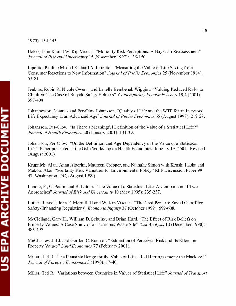
30

1975): 134-143.

Hakes, Jahn K. and W. Kip Viscusi. “Mortality Risk Perceptions: A Bayesian Reassessment”Journal of Risk and Uncertainty 15 (November 1997): 135-150.

Ippolito, Pauline M. and Richard A. Ippolito. “Measuring the Value of Life Saving fromConsumer Reactions to New Information” Journal of Public Economics 25 (November 1984):53-81.

Jenkins, Robin R, Nicole Owens, and Lanelle Bembenek Wiggins. “Valuing Reduced Risks toChildren: The Case of Bicycle Safety Helmets” Contemporary Economic Issues 19,4 (2001):397-408.

Johannesson, Magnus and Per-Olov Johansson. “Quality of Life and the WTP for an IncreasedLife Expectancy at an Advanced Age” Journal of Public Economics 65 (August 1997): 219-28.

Johansson, Per-Olov. “Is There a Meaningful Definition of the Value of a Statistical Life?”Journal of Health Economics 20 (January 2001): 131-39.

Johansson, Per-Olov. “On the Definition and Age-Dependency of the Value of a StatisticalLife” Paper presented at the Oslo Workshop on Health Economics, June 18-19, 2001. Revised(August 2001).

Krupnick, Alan, Anna Alberini, Maureen Cropper, and Nathalie Simon with Kenshi Itaoka andMakoto Akai. “Mortality Risk Valuation for Environmental Policy” RFF Discussion Paper 99-47, Washington, DC, (August 1999).

Lanoie, P., C. Pedro, and R. Latour. “The Value of a Statistical Life: A Comparison of TwoApproaches” Journal of Risk and Uncertainty 10 (May 1995): 235-257.

Lutter, Randall, John F. Morrall III and W. Kip Viscusi. “The Cost-Per-Life-Saved Cutoff forSafety-Enhancing Regulations” Economic Inquiry 37 (October 1999): 599-608.

McClelland, Gary H., William D. Schulze, and Brian Hurd. “The Effect of Risk Beliefs onProperty Values: A Case Study of a Hazardous Waste Site” Risk Analysis 10 (December 1990):485-497.

McCluskey, Jill J. and Gordon C. Rausser. “Estimation of Perceived Risk and Its Effect onProperty Values” Land Economics 77 (February 2001).

Miller, Ted R. “The Plausible Range for the Value of Life - Red Herrings among the Mackerel”Journal of Forensic Economics 3 (1990): 17-40.

Miller, Ted R. “Variations between Countries in Values of Statistical Life” Journal of Transport

31

Economics and Policy 34,2 (May 2000): 169-188.

Moore, M.J. and W.K. Viscusi. “The Quantity-Adjusted Value of Life” Economic Inquiry 26(1988): 369-88.

Mount, Timothy, Weifeng Weng, William Schulze, and Laurie Chestnut. “Automobile Safetyand the Value of Statistical Life in the Family: Valuing Reduced Risk for Children, Adults, andthe Elderly” Presented at the Association of Environmental and Resource Economists Workshop“Assessing and Managing Environmental and Public Health Risks” in Bar Harbor, ME, on June13-15, 2001.

Mrozek, Janusz R. and Laura O. Taylor. “What Determines the Value of Life? A Meta-Analysis”Journal of Policy Analysis and Management (forthcoming 2002).

O’Conor, Richard M. and Glenn C. Blomquist. “Measurement of Consumer-Patient PreferencesUsing a Hybrid Contingent Valuation Method” Journal of Health Economics 16 (December1997): 667-83.

Portney, Paul R. “Housing Prices, Health Effects, and Valuing Reductions in Risk” Journal ofEnvironmental Economics and Management 8 (March 1981): 72-78.

Quiggin, J. “Risk, Self-Protection, and Ex Ante Economic Value - Some Positive Results”Journal of Environmental Economics and Management 23 (July 1992): 40-53.

Rosen, Sherwin. “The Value of Changes in Life Expectancy” Journal of Risk and Uncertainty 1(September 1988): 285-304.

Shogren, Jason and Thomas D. Crocker. “Risk and Its Consequences” Journal of EnvironmentalEconomics and Management 37 (January 1999): 44-51.

Shogren, Jason and Thomas D. Crocker. “Risk, Self-Protection, and Ex Ante Economic Value”Journal of Environmental Economics and Management 20 (1991): 1-15.

Shogren, Jason and Tommy Stamland. “Skill and the Value of Life” Presented at theAssociation of Environmental and Resource Economists Workshop “Assessing and ManagingEnvironmental and Public Health Risks” in Bar Harbor, ME, on June 13-15, 2001.

Smith, V. Kerry. “Household Production Functions and Environmental Benefit Estimation” inJ.B. Braden and C.D. Kolstad Measuring the Demand for Environmental Quality (New York,NY: North Holland, 1991).

Smith, V. Kerry, Donald J. Epp, and Kurt A. Schwabe. “Cross-Country Analyses Don’t EstimateHealth-Health Responses” Journal of Risk and Uncertainty 8 (January 1994): 67-84.

32

Smith, V. Kerry and Carol C.S. Gilbert. “The Valuation of Environmental Risks Using HedonicWage Models” in Martin David and Timothy Smeeding, eds., Horizontal Equity, Uncertainty,and Economic Well-Being (Chicago: University of Chicago Press for NBER, 1985): 359-85.

Smith, V. Kerry, Hyun Kim and Donald H. Taylor, Jr. “Do the ‘Near’ Elderly Value MortalityRisks Differently?” Presented at the Association of Environmental and Resource EconomistsWorkshop “Assessing and Managing Environmental and Public Health Risks” in Bar Harbor,ME, on June 13-15, 2001.

Smith, V. Kerry and Ju-Chin Huang. “Can Markets Value Air Quality? A Meta-analysis ofHedonic Property Models” Journal of Political Economy 103 (February 1995): 209-227.

Smith, V. Kerry and F. Reed Johnson. “How Do Risk Perceptions Respond to Information? TheCase of Radon” Review of Economics and Statistics 70 (February 1988): 1-8.

Stanley, T.D. “Wheat from Chaff: Meta-Analysis as Quantitative Literature Review” Journal ofEconomic Perspectives 15 (Summer 2001): 131-150.

Sunstein, Cass R. “Bad Deaths” Journal of Risk and Uncertainty 14 (May-June 1997): 259-82.

Viscusi, W. Kip. “The Value of Risks to Life and Health” Journal of Economic Literature 31(December 1993): 1912-1946.

Viscusi, W. Kip. “Risk-Risk Analysis” Journal of Risk and Uncertainty 8 (January 1994): 5-17.

Viscusi, W. Kip, Jahn K. Hakes, and Alan Carlin. “Measures of Mortality Risks” Journal of Riskand Uncertainty 14 (May-June 1997): 213-233.

Viscusi, W. Kip and William N. Evans. “Estimation of Revealed Probabilities and UtilityFunctions for Product Safety Decisions” Review of Economics and Statistics 80 (February 1998):28-33.

Viscusi, W.K., W.A. Magat, and J. Huber. “Smoking Status and Public Responses to AmbiguousScientific Risk Evidence” Southern Economics Journal 66,2 (1999): 250-70.

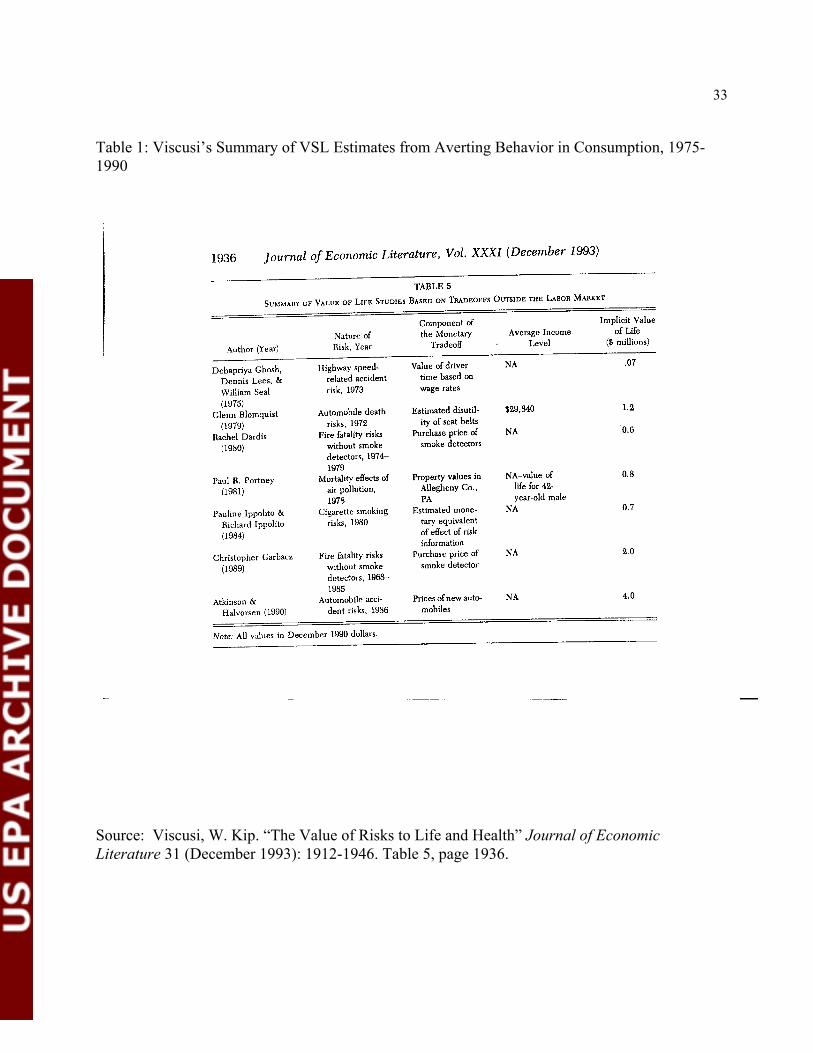
33

Table 1: Viscusi’s Summary of VSL Estimates from Averting Behavior in Consumption, 1975-1990

Source: Viscusi, W. Kip. “The Value of Risks to Life and Health” Journal of EconomicLiterature 31 (December 1993): 1912-1946. Table 5, page 1936.

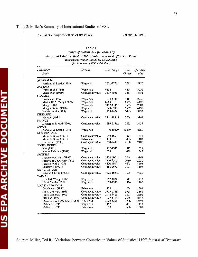
35

Table 2: Miller’s Summary of International Studies of VSL

Source: Miller, Ted R. “Variations between Countries in Values of Statistical Life” Journal of Transport

36

Economics and Policy 34,2 (May 2000): 169-188. Table 1, page 34.

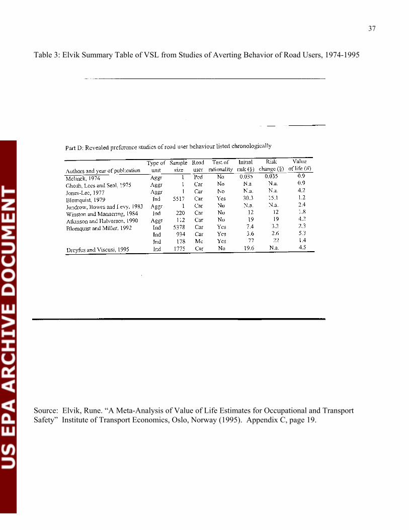
37

Table 3: Elvik Summary Table of VSL from Studies of Averting Behavior of Road Users, 1974-1995

Source: Elvik, Rune. “A Meta-Analysis of Value of Life Estimates for Occupational and TransportSafety” Institute of Transport Economics, Oslo, Norway (1995). Appendix C, page 19.

38

Table 4: de Blaeij et al.’s Summary of Averting Behavior of Road Users, 1973-1999

Source: de Blaeij, Arianne, Raymond J.G.M Florax, Piet Rietveld, and Erik Verhoef. “The Value ofStatistical Life in Road Safety: A Meta-Analysis” Tinbergen Institute Discussion Paper, TI 2000-089/3,(2000). Table 1, page 31.

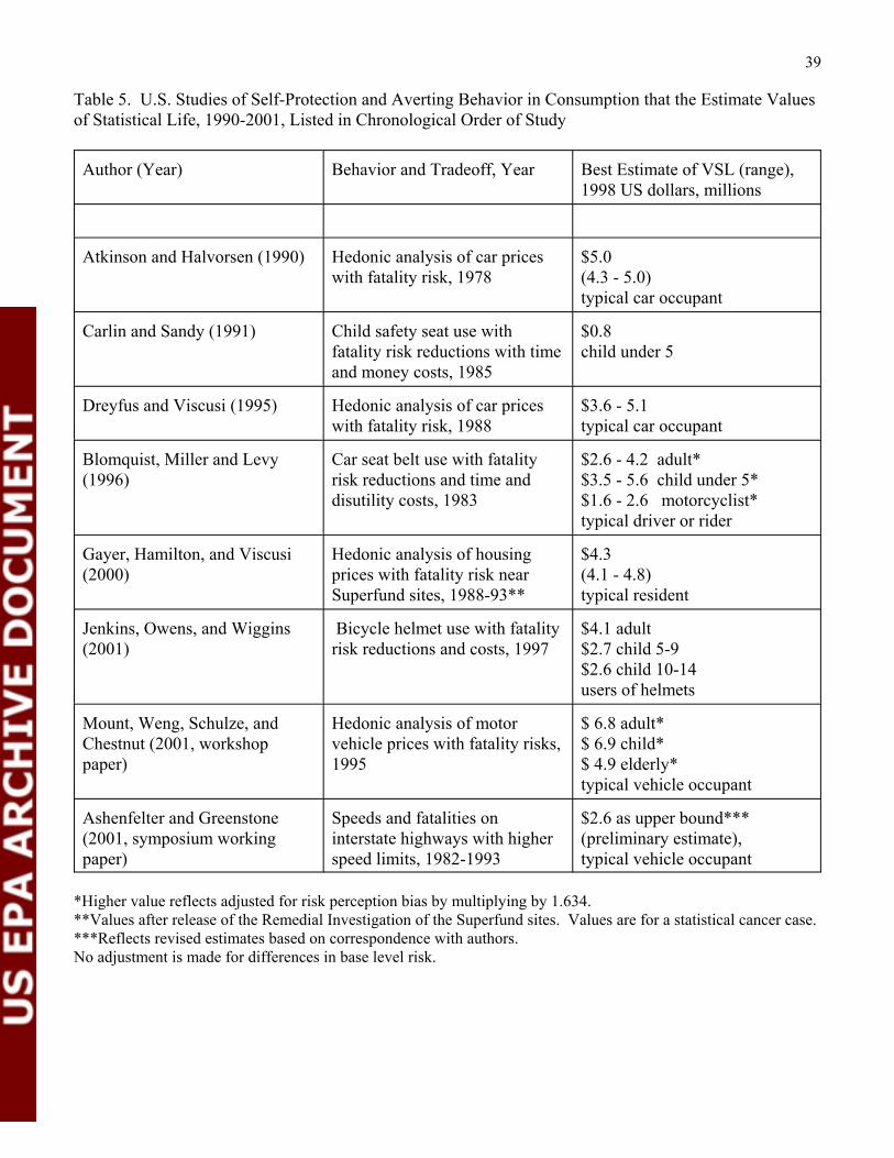
39

Table 5. U.S. Studies of Self-Protection and Averting Behavior in Consumption that the Estimate Valuesof Statistical Life, 1990-2001, Listed in Chronological Order of Study

Author (Year) Behavior and Tradeoff, Year Best Estimate of VSL (range),1998 US dollars, millions

Atkinson and Halvorsen (1990) Hedonic analysis of car priceswith fatality risk, 1978

$5.0(4.3 - 5.0)typical car occupant

Carlin and Sandy (1991) Child safety seat use withfatality risk reductions with timeand money costs, 1985

$0.8 child under 5

Dreyfus and Viscusi (1995) Hedonic analysis of car priceswith fatality risk, 1988

$3.6 - 5.1 typical car occupant

Blomquist, Miller and Levy(1996)

Car seat belt use with fatalityrisk reductions and time anddisutility costs, 1983

$2.6 - 4.2 adult*$3.5 - 5.6 child under 5*$1.6 - 2.6 motorcyclist*typical driver or rider

Gayer, Hamilton, and Viscusi(2000)

Hedonic analysis of housingprices with fatality risk nearSuperfund sites, 1988-93**

$4.3(4.1 - 4.8)typical resident

Jenkins, Owens, and Wiggins(2001)

Bicycle helmet use with fatalityrisk reductions and costs, 1997

$4.1 adult$2.7 child 5-9$2.6 child 10-14users of helmets

Mount, Weng, Schulze, andChestnut (2001, workshoppaper)

Hedonic analysis of motorvehicle prices with fatality risks,1995

$ 6.8 adult*$ 6.9 child*$ 4.9 elderly*typical vehicle occupant

Ashenfelter and Greenstone(2001, symposium workingpaper)

Speeds and fatalities oninterstate highways with higherspeed limits, 1982-1993

$2.6 as upper bound***(preliminary estimate),typical vehicle occupant

*Higher value reflects adjusted for risk perception bias by multiplying by 1.634.**Values after release of the Remedial Investigation of the Superfund sites. Values are for a statistical cancer case. ***Reflects revised estimates based on correspondence with authors.No adjustment is made for differences in base level risk.

104

Discussion of Session I Bryan Hubbell, US EPA Office of Air Quality Planning and Standards

Introduction There are three major methods for estimating the value of reducing mortality risks, or in the common shorthand, the value of a statistical life. These methods include stated preference (contingent valuation, stated choice, etc.), hedonic wage-risk, and averting behavior. By far the most common method used to date has been the hedonic wage-risk method. The paper by Black, Choi, and Walker provides an interesting set of potential biases in these analyses and proposes an interesting non-parametric statistical treatment to reduce the influence of some of these sources of bias. Glen Blomquist seeks to breath new life into the other revealed preference method, averting behavior, a source of VSL estimates that has been mostly downplayed in policy analysis. Anna Alberini provides an overview of a new research effort to bring older stated preference studies into the present by reanalyzing their data with new statistical methods. I’ve been asked to provide a policy perspective on these two papers, and in order to provide some context for my comments, let me begin by arguing for more attention to semantics. In my presentations to policymakers, one of the most misunderstood concepts is the statistical life. Perhaps the most important education we can provide for policymakers if we wish to continue to refine values of fatal risk reduction for policy use is to avoid the value of life terminology. For policy analysis, we are almost always valuing small changes in the risk of death, not valuing lives. We apply the VSL aggregation to avoided “statistical death,” but in essence, these are merely aggregations of population changes in the risk of death. What Are Policymakers Looking For? Most policymakers understand that we are reducing risk for large populations, but when we present them with statistical lives saved, and values of statistical lives saved, or as each paper does on at least one occasion, refer to the value of life, the immediate reaction is that we are saving lives, which implies that somehow, we could go out and find the individuals whose lives will be prolonged by our policies. I believe that policy and academics would be much better served if we referred to the magnitude of reduced risk and the size of the population affected, rather than going through the statistical aggregation to “statistical lives saved”. The value would be the same, but it would be the value of a risk reduction for a large population rather than the value of “lives saved,” which seems to have a much larger moral connotation. An explicit reminder that we are reducing the risk of death and not intervening to save specific lives would, I think, go a long way towards reducing the distaste many policymakers feel towards valuing fatal risk reductions as a part of the policy evaluation process. Policymakers have several issues with the current mortality risk literature. First, policymakers don’t like to deal with very uncertain numbers. The wide range of VSL estimates in the literature, and the lack of agreement about the reliability of those estimates, even within the economics discipline, causes policymakers to discount the usefulness of valuation in

105

evaluating policies. Second, because we are focused on the “lives saved” and “value of lives” terminology, policymakers are reluctant to assign different values for lives saved based on age, income, risk type, or other demographic characteristics. All of these papers may help to reduce the unexplained variability in estimates of the value of fatal risk reductions. And, if we can move away from the “value of life” terminology, all of these papers can potentially help in understanding how variability in values relates to underlying characteristics of the risk and population affected. Key Points from the Papers Black, Choi, and Walker: “Some Problems in the Identification of the Price of Risk” Starting with the paper on hedonic wage-risk analysis, Black and coauthors list 5 problems in the measurement of job risk that may bias the estimate of the estimated implicit value of fatal risk reductions. Of these, only one, measurement error in assigning job risks, has a clear downwards bias, while the other 4 can lead to biases of unknown magnitude and direction. The potentially large downward bias caused by measurement error also has implications for the averting behavior literature, because objective risk measures are often used to calculate VSL in these studies. To the extent that averting behavior studies are ex-post analyses of consumer purchases, unless the risk measure is an ex-ante estimate of risk (prior to the consumer purchases), the estimated risk will be endogenously determined, and will be the outcome of a similar random process. The second major problem, correlation between job risks and unobserved job and worker characteristics, may be resolved if sources of exogenous risk change can be found. Black and coauthors cite he work by William Evans on transportation accident rates and impact of drunk driving laws. This suggests that time series of job risk for individual jobs may need to be construc ted. However, it should be verified that employers are able to offer lower wages to currently employed workers when safety improvements are implemented. If wages are upwardly sticky, so that workers in a given job in a particular age cohort are not likely to see wages fall commensurately with risk, then it will not be possible to relate temporal changes in risk with temporal changes in wages to recover WTP for the risk change. For example, one would need to see if employers were able to reduce wages based on implementation of new safety regulations. An important research question is are there other “natural experiments” that can be exploited to examine changes in risk and wages within a given industry?

Based on recent statements by the Office of Management and Budget, there is likely to be renewed interest in reporting fatal risk reductions in terms of increases in life expectancy or increases in life-years, rather than statistical lives. Current wage-risk studies do not provide information on the value of life-years or life-expectancy, however, the non-parametric approach may allow recovery of age-specific values of risk reduction, which could be used in valuing changes in life-expectancy or life-years.

106

Are wage-risk studies useful if we move to a life-years or longevity framework? Even if wage-risk studies were able to provide unbiased, efficient estimates of VSL, some analysts in the U.S. and Europe, such as Graham Loomes, are suggesting that we couch risk reductions in terms of increases in longevity, or increases in QALY’s, or other non-binary outcomes. This would require a great deal of additional data on the age distribution of workers in particular industries and on age-specific risks. For example, it is highly unlikely that risk in a particular industry are age independent, partly due to movement from labor to management over time, partly due to skill in avoiding risk, partly due to self-selection, and partly due to industry desires to minimize risks. As older workers lose physical dexterity, they may be forced into earlier retirement or into less risk intensive duties. And, because of the limited age range covered by wage-risk studies, they cannot provide estimates of WTP for the population over 65. In addition to the bias issues raised by Black and coauthors, there are also two relatively new issues. The first is the concern raised by Shogren and Stamland about heterogeneity among workers with unobservable differences in skill at avoiding risks. They indicate this may lead to overestimates of VSL based on observed wage-risk tradeoffs. The second issue is in regards to the effects of relative income on wage-risk tradeoffs. This interesting issue, raised by Frank and Sunstein, implies that VSL for environmental policy applications may be understated by up to 50 percent. Both of these additional issues only add to the uncertainty surrounding wage-risk based VSL estimates. While the non-parametric approach described by Black and coauthors may help provide age specific estimates of the value of risk reduction, there may still be inherent selection biases, if older individuals opt out of dangerous jobs so that remaining employees are not a representative sample of that age cohort. In addition to the issues with risk measurement raised by Black and coauthors there are also other problems with wage-risk based estimates, such as the problem of relative income levels as raised by Frank and Sunstein, or the skill-sorting problem raised by Shogren. This raises the question of whether the additional information that can be gained from further refinement of the wage-risk literature is worth the potentially substantial investment of research dollars that would be necessary to achieve that information. And, how should the new information be viewed relative to existing data? The recent meta-analyses by Mrozek and Taylor suggest some ‘best practices’, but these need to be examined carefully, as they have rather large implications for the mean value of risk reductions.

Blomquist: “Self Protection and Averting Behavior, Values of Statistical Lives, and Benefit Cost Analysis of Environmental Policy”

Blomquist’s paper is focused on averting behavior models. These models have generally not been used in EPA’s valuation of fatal risk reductions, mainly due to concerns about the ability of these studies to provide an unbiased estimate of VSL and the tendency to underestimate VSL relative to WTP based measures. However, average VSL values cited by

107

Blomquist are within the range of estimates from CV and hedonic wage studies used by EPA in recent analyses. Blomquist also raises the issue of why averting behavior based estimates are higher than the range of estimates suggested by Mrozek and Taylor’s ‘best practice’ estimates. I would suggest that more attention needs to be given to the definitions of best practice provided by that study. The low estimates suggested by Mrozek and Taylor are driven largely by an adjustment reflecting whether studies included more than four dummy variables for occupation. To the extent that occupation is correlated with job risk, including dummy variables for occupation may overadjust for the effects of occupation, leading to a downward bias in the estimated coefficient on job risk. For the purpose of checking the robustness of risk-wage relationships, this may be appropriate. However, for purposes of establishing a VSL for policy analysis, we want an unbiased estimate, not one that has been constructed to control for occupational differences at the expense of unbiasedness. He also raises the issue of the impact of unobservable heterogeneity in risk reducing skills by laborers as a reason to suspect wage-risk based estimates should be even lower (Shogren and Stamland). However, while theoretically interesting, the magnitude of this effect has not been shown empirically. Blomquist calls special attention to a study by Ashenfelter and Greenestone (2001) which looked at the impact of increased speed limits and derived an implied value of risk by looking at tradeoffs in time gained and life lost. However, this is an ex post evaluation looking at the implied risk from realization of a random event, when individuals were functioning with incomplete information on actual risks from the higher speeds. The problem with this study is that the measure of risk, obtained by looking at observed fatalities, is in itself a reduced form measure which is a function of perceived risk and mitigating behavior on the part of drivers (this problem was also noted by Black for the hedonic wage literature, where he suggests the potential for downward bias). Blomquist also discusses the need to correctly account for perceived risks when calculating VSL based on averting behavior. The same argument holds true for wage-risk studies, although Mrozek and Taylor find little evidence of a strong impact of using self-reported risk instead of objective risk estimates. Blomquist discusses several recent studies which attempt to derive a value for reducing risks of death for children. The real question is “Are the private decisions of parents regarding children’s safety an adequate measure of society’s preferences for children’s safety?” Given that many states have bicycle helmet laws and child safety seat laws, it could be argued that parents who would have chosen not to consume these products are now buying them, so that these are constrained choices reflecting societal preferences as well as personal choices. Averting behavior studies may provide interim values that can be used in current regulatory analyses. However, long term research may need to address whether the current parental value paradigm is appropriate for regulatory benefit-cost analysis.

108

So what is the future of averting behavior/consumer market analysis as a source of VSL estimates? Regardless of the quality of the study, averting behavior studies can in most cases only produce a lower bound estimate when based on consumer purchases. However, they may be useful because they can focus on specific risks to specific sub-populations, which hedonic wage studies cannot, since they rely on aggregate data from only the working age population. Also, because they can focus on specific risk reducing products, there is potentially less chance for confounding than hedonic wage-risk studies, where wages may reflect a large number of factors other than fatal risk.

Alberini: “Willingness to Pay for Mortality Risk Reductions: A Re-examination of the Literature”

Alberini raises some interesting questions in her proposed research. Several of the robustness criteria deal with “contamination” by yea-saying, nay-saying, and random responses. She also raises the issue of potential sample selection bias. One critical issue for environmental policy analysis is obtaining a reliable estimate of WTP for risk reductions for the elderly, especially those over the age of 80. Figure 1 shows the distribution of the prolonged lives from reducing particulate matter resulting from the recent Heavy Duty Diesel rule and emphasizes why this is important. Around 40 percent of estimated mortality benefits are due to reducing mortality risks for those over 80 years of age. It seems likely that individuals in this age category may be less likely to respond to surveys and that if they do respond, they may seek assistance in responding or may systematically have more difficulty in understanding complex new information, such as risk probabilities. Special care will need to be taken in obtaining values for this class of individuals. In addition to treatment of zero WTP responses, care needs to be taken in determining how “don’t know” responses are treated. In some cases, a don’t know” may truly be an indication that the respondent does not have well constructed preferences for the risk reduction. In other cases, a don’ t know may be a cry for help, looking for additional understanding of the risk prior to making a commitment of resources. In fact, the more the respondent buys into the hypothetical market, the more likely the individual is to respond with a need for more information, especially as bid amounts increase. In a recent analysis by Krupnick et al., “don’t know”s were treated as no’s, which may lead to a significant downward bias in estimated VSL. A better understanding of why individuals respond with “don’t know” would be useful. And, I do not believe simply omitting “don’t know” as a response solves the problem, as you are then forcing people to choose with limited information, potentially increasing the probability of nay-saying. How will each of these approaches address the pressing policy questions of the near future? In addition to the many issues raised in each of the papers, research into the value of reducing risks from environmental pollution will need to address some very important issues in the near future. Regulatory analysts are being asked to provide measures not only of lives saved,

109

but of quality adjusted life years saved, increases in life expectancy, and impacts for specific age categories, especially the very young and very old. Each of the three methods needs to be evaluated for how well it can provide answers to these questions. In addition, research is needed to examine the impact of not only income or wages, but also of wealth. John Graham has questioned whether the higher values for risk reductions in the elderly observed in some studies is due to the higher levels of wealth for this age class, even though income levels are lower. Most hedonic wage, averting behavior, and stated preference studies have included income, but not wealth as an explanatory variable. Finally, what do we do with old estimates? Do we begin to throw out those that do not pass a minimum quality standard, or do we, as Anna Alberini suggests, go back to the data and revitalize it with new statistical methods? This is an important question not only for fatal risk valuation, but also for other morbidity and environmental endpoints. Given the scarcity of high quality studies providing values for many health and environmental effects, the ability to bring some older studies back to life would greatly enhance our ability to conduct benefits analyses.

110

Figure 1. Age Distribution of Avoided Premature Mortalities from the Heavy Duty Engine/Diesel Fuel Rule

0

500

1000

1500

2000

2500

30-39 40-59 60-69 70-79 80-84 85+

Age Category

Num

ber

of P

rem

atur

e M

orta

litie

s

111

Discussion of Session I Ted R. Miller, Pacific Institute for Research and Evaluation Comments on Dan Black’s Paper In reading Dan Black’s paper, I wondered about the wisdom of using an instrumental variable that is a good explanator of the Stage 2 dependent variable. It seems to me that approach will yield biased value estimates. A much better choice might be to try the days required to qualify for Worker’s Compensation as an instrument. I also was struck by the paper’s discussion of two U.S. occupational death data sets; which ignored the data set that many now consider the gold standard—the Census of Fatal Occupational Injuries (CFOI). The extant data sets are • National Traumatic Occupational Fatalities (NTOF), a National Institute on

Occupational Safety and Health census collected from 1980 to the present, with New York City missing in early years because its death certificates did not code whether deaths were work-related. NTOF collects occupation, industry, and state of residence for every victim. Although a detailed occupation by industry risk table is available from NIOSH, through 2000, studies using NTOF to analyze wage compensation for occupational risk all used a risk table by region and very aggregated industry instead. That choice was questionable.

• The Census of Fatal Occupational Injuries (CFOI) from the Bureau of Labor Statistics (BLS) is available by occupation & industry from 1992 to the present. Its counts are close to, but a bit higher than NTOF counts because it captures occupational deaths from other sources as well as death certificates.

• The BLS Annual Survey fatality counts by occupation and industry, which were discontinued after 1991 due to undercount problems. This data set, unlike NTOF and CFOI, does not cover all workers. Exclusions include the self-employed and government workers.

It strikes me as odd to continue focusing analyses on old BLS data discontinued because of inaccuracy problems when current and reasonably accurate data are readily available. Problems arise even with the current data. First occupational injury death is a rare event, so multi-year averages are needed to get accurate risk estimates. The occupational injury death rate has dropped precipitously in the last decade, however, so averaging across years may be dicey. Perhaps we should average wages over the same period. Second, occupational deaths also result from chronic illness. The data snapshot only a subset of the deaths, hardly a desirable property for a critical dependent variable. A partial solution here might be to access unpublished CFOI data on illness deaths, a source that Paul Leigh has been exploring. Third, whatever data set one uses, the analysis needs to account for nonfatal risk as well as fatality risk. Because of multi-collinearity, as described below, the best approach probably is to use expected Quality-Adjusted Life Year (QALY) loss by occupation and industry as the risk variable. The only injury risk data available are the BLS Annual Survey data. Regrettably, they exclude large classes of workers and are suspected of undercounting injuries to included workers.

112

The occupational motor vehicle death analysis that Black suggests seems a good idea BUT it has one major, potentially insurmountable problem. Many occupational motor vehicle deaths are drivers in interstate commerce, long-haul truck and bus drivers and even taxi drivers in the many metropolitan areas that straddle state borders. What state(s) should we assign each driver to? Again, it would be critical to consider nonfatal injury risk and perhaps even the risk of no- injury crashes in this analysis. QALY-based Risk Variables. A QALY is a health outcome measure that assigns a value of 1 to a year of perfect health and 0 to death. To get the QALY losses associated with an adverse health event, we sum the fraction of perfect health lost each year due to that event. In the best recent literature on QALYs, one accounts for health decline with age, so death causes the loss of less than one QALY per life year lost (Gafni 1991 ????). The consensus in the literature is that QALYs should be discounted to present value (e.g., Cropper et al. 1991, 1992; Viscusi 1995; Agee and Crocker 1996), in part because advancing medical technology may reduce the expected effects of chronic or “permanent” impairment. Working from economic theory, Miller, Calhoun and Arthur (1989) demonstrates that QALYs are an appropriate way to include fatal and nonfatal losses simultaneously in valuing health outcomes. Miller et al. (1995) and Miller (JFE, 2001) detail the mechanics involved. A monetized QALY approach underlies the fatality equivalents that the National Highway Traffic Safety Administration uses in its regulatory analyses and the willingness-to-pay values for injury used elsewhere at he US Department of Transportation (Miller, Luchter and Brinkman 1989; Miller et al. 1991; Miler 1993; Miller et al. 1995; Blincoe 1996). Our QALY methods are detailed further in the documentation of the US Consumer Product Safety Commission’s injury cost model (Miller at al. 1998; available on request to William Zamula at CPSC, 301-504-0962, [email protected] ). CPSC chose to use values of non-fatal injury derived from regression analysis of the non-economic component of jury verdicts, but validated those values against our QALY-based estimates. Cohen and Miller (under review) and Smith (2001) detail several analyses that used our QALY estimates to explain jury awards for non-fatal injury. These analyses suggest that juries use a VSL $2 to $4 million to value QALY loss, with the higher end of this range used to value losses to victims of violence and impaired driving and the lower end used to compensate vic tims of consumer product injury. Virtually all the U.S. data sets used to develop wage-risk estimates of the value of statistical life (VSL), including the Current Population Survey, the Quality of Employment Survey, and the Panel Study of Income Dynamics, are weighted sample surveys. Yet those data sets generally were analyzed with statistical packages that systematically underestimate standard deviations in weighted data. Either they ran regressions on the unweighted data or used weighted regression routines in BMD, SAS or SPSS that did not use jackknife or bootstrap procedures. In either event, unless analysts used SUDAAN, WESVAR, or LIMDEP (or more recently STATA or a new SAS module released in 2000) and brought in the sample design, the analyses underestimate standard deviations and overestimate coefficient significance. At the time these analyses were run,

113

SUDAAN either did not exist or required much expense and training to use. Not surprisingly, none of he analyses correctly handled the weights. The poor man's way to reduce the weighting problem would be to analyze the unweighted data and include the stratifiers in the regression equation. I do not think that approach was used either. This problem also applies to some regression-based VSL estimates from behavior, notably the Blomquist et al. estimates from the National Personal Transportation Survey. To illustrate the potential impact, in a recent log- linear analysis of motor vehicle crash injury costs, we set up the data set in SAS and ran a weighted regression, then transferred the data to STATA to get standard deviations right. The coefficient estimates in the model, of course, did not change. The significance of our main variable of interest, however, went from 0.005 to 0.33 and adjusted r-squared dropped from 0.36 to 0.28. This problem with the standard deviations is especially important for the Kochi,

Hubbell & Kramer (2000) Bayesian VSL meta-analysis. That analysis depends critically

on the incorrectly estimated effect sizes.

Comments on Anna Alberini’s Paper Alberini proposes to reanalyze some oft-cited past surveys on the value of fatal risk reduction. Much of her emphasis is on better handling of discrete-choice survey bids. That emphasis is confusing since the contingent valuation surveys she mentions generally used open-ended bidding. Moreover, both Hammitt & Graham (1999) and Beattie et al. (1998) already taught us many of these surveys have serious design flaws, so I am unsure how much we can learn from a reanalysis. In particular, most of them used 1 in 100,000 risk levels that apparently were too small for respondents to understand. Nevertheless, if one can get access to the data, Viscusi, Magat & Huber (1989) may be worth reanalyzing because it did not handle outliers well. Miller & Guria (1992) is analyzed with much attention to outliers but some reanalysis may make sense because the authors lacked the tools now available to do weighted regression and never fully integrated their contingent valuation data with longitudinal travel diary data collected from the same respondents. Gerking analyzed the data that his team collected extensively and thoughtfully but they are fine data. Some limited reanalysis may make sense, but only if the analyses planned can advance what we already learned from this data set. The Jones-Lee data are not readily available, but even if they were, I think this reasonably early survey had too many design warts for a reanalysis to be worthwhile. I noticed that Alberini’s partial draft did not cite the Schwab-Christe (1995) book full of European estimates or the subsequent estimates published in the Journal of Transport Economics & Policy or Journal of Risk and Uncertainty. Those references include several discrete choice surveys that might be better suited to the analyses she proposes.

114

Finally, with respect to the surveys, I think we can design a lot better. The recent Resources for the Future work that Alberini, Alan Krupnick, and others have undetaken is certainly a step in the right direction. Another tack, which might be more workable is time-risk trade-off questions (discussed further below). Miller & Guria (1992), Persson, and Jara-Diaz (2000) have used this approach. The later two studies, are particularly interesting as they build on the block choice designs that have proven so successful in modal choice modeling. Some of the best survey-based VSLs come from polling respondents about behavior and perceived risk change, not contingent values (CV) directly. They then use the data to estimate how respondents value risk reduction. This approach avoids the very difficult problem of creating realistic CV questions without using risk changes too small for respondents to understand. It also avoids having to make the recurring, and in my opinion always foolish, CV assumption that respondents will ignore nonfatal health effects if the interviewer tells them too. That violates the tenets of a realistic scenario. In the real world, nonfatal and fatal cases are the severity continuum of consequences from a single incident. People are too smart to believe that you can prevent highway crash deaths without having any impact on other injuries in crashes. Comments Stimulated by Glenn Blomquist’s Paper This paper talks about the existing meta-analyses on VSL, but it does not describe the characteristics of a good meta-analysis. That gives me something to discuss. A good meta-analysis should: • Considers all values from each study • Account for serial correlation of the values in each study (or data set combination

used across two or more studies) • Fix fixable problems before analyzing (e.g., converting to a uniform value of travel

time and discount rate, correcting a VSL that the original author extracted incorrectly from a regression equation, adequately dealing with absurd bids in CV studies) or code for problems, knowing a priori, which code value is theoretically correct and will be used to extract the consensus estimate from the VSL regression equation (e.g., before tax versus after-tax value; all-mortality risk used with compensation data for work-related risk only, implicitly bundles the value of non-fatal risk reduction into the value of fatal risk reduction). Note that some of these have a multiplicative impact on the VSL and cannot be accounted for simply by coding a dummy variable

• Searches for and includes unpublished studies • Does not discount or ignore studies that found no willingness-to-pay (WTP) for

fatality risk • Excludes extraneous concepts (e.g., what government spent on safety, the threshold

value of life below which people would not rationally purchase a product) • Excludes seriously flawed analyses (notably surveys with really bad design flaws or

just half a dozen respondents) or finds ways to let the meta-analysis decide whether to discount/ignore these studies

115

The Mrozek & Taylor wage-risk meta-analysis gets an A by these criteria. Miller (1990) gets a B-. it was a valiant effort for its time period but it did not apply regression and it fixed some problems somewhat arbitrarily that might better have been adjusted for using regression. Miller (2000) also gets a B- because it does not add newer US studies and does not code multiple values from each study. De Blaeij et al. (2001) ultimately should get a good grade, but the current draft includes studies that are not studies of individual WTP, -which makes it unacceptable. Desvousges et al. (1998) gets a low grade for omitting far too many studies. The Industrial Economics study presented at this meeting, on the other hand, gives too much value to really bad studies. In contrast, the second meta-analysis presented excludes any study that found a zero-WTP, thus guaranteeing an overestimate of the all-study value. It also is not sufficiently discriminating about flawed studies that got non-zero values, often very high ones. The other reviews I have seen, e.g., Viscusi (1993), are not meta-analyses or critical literature syntheses. Another issue concerns the fact that virtually all the U.S. data sets used to develop wage-risk estimates of the value of statistical life (VSL), including the Current Population Survey, the Quality of Employment Survey, and the Panel Study of Income Dynamics, are weighted sample surveys. Yet those data sets generally were analyzed with statistical packages that systematically underestimate standard deviations in weighted data. Either they ran regressions on the unweighted data or used weighted regression routines in BMD, SAS or SPSS that did not use jackknife or bootstrap procedures. In either event, unless analysts used SUDAAN, WESVAR, or LIMDEP (or more recently STATA or a new SAS module released in 2000) and brought in the sample design, the analyses underestimate standard deviations and overestimate coefficient significance. At the time these analyses were run, SUDAAN either did not exist or required much expense and training to use. Not surprisingly, none of he analyses correctly handled the weights. The poor man's way to reduce the weighting problem would be to analyze the unweighted data and include the stratifiers in the regression equation. I do not think that approach was used either. This problem also applies to some regression-based VSL estimates from behavior, notably the Blomquist et al. estimates from the National Personal Transportation Survey.

To illustrate the potential impact, in a recent log- linear analysis of motor vehicle crash injury costs, we set up the data set in SAS and ran a weighted regression, then transferred the data to STATA to get standard deviations right. The coefficient estimates in the model, of course, did not change. The significance of our main variable of interest, however, went from 0.005 to 0.33 and adjusted r-squared dropped from 0.36 to 0.28. This problem with the standard deviations is especially important for the Kochi, Hubbell & Kramer (2000) Bayesian VSL meta-analysis. That analysis depends critically on the incorrectly estimated effect sizes. Blomquist’s paper primarily focuses on published consumer behavior studies. These studies have several consistent problems, many of which were fixed in Miller (1990). Current meta-analyses should use the consumer behavior values from that study in place of the original values. It not only introduces consistent discount rates and values of time

116

but accounts carefully for the impacts on nonfatal injury. It adjusts for risk perception, an adjustment that Miller (2000) more wisely does meta-analytically. Miller (1990) contains a series of new consumer behavior estimates, often identifying them with the name of a study of consumer behavior that provided information needed to derive a VSL. In retrospect, too many people have failed to find those values. I should have labeled Miller (1990) as their source. Virtually everything written about consumer behavior studies, including most estimates in Miller (1990), has confused the VSL threshold at which a purchase is rational or the VSL below which people actually do not purchase a good with the average VSL. For example, a recent article on bicycle helmets (Jenkins et al. 2001) has been widely misinterpreted as saying people value their children less than themselves. Instead, it probably implies just the opposite. It says people use a much lower threshold VSL to justify buying bicycle helmets for their children than for themselves. Since many more children than adults have bicycle helmets, that probably means parents value their children more than themselves. To know for sure, we need to know the shape of the safety demand curve, not just one point on it. Again, Dardis’ oft-cited (1980) VSL estimate for smoke detectors simply reflects a threshold VSL for those who bought at a certain price. Many of those buyers had higher VSLs and realized a consumer surplus. Using data on price versus purchase frequency, Miller (1990) was able to integrate under the demand curve, obtaining an estimate of the mean VSL across US households. Interestingly, as Figure 1 illustrates, the demand curve for smoke detectors in the US (adjusted for risk misperception) is virtually identical to the safety demand curve from my CV survey about highway safety in New Zealand (Miller and Guria 1992). I am very fond of time-risk tradeoff studies and was interested to see that a new one on speed choice is circulating. Safety behavior generally involves trading safety against money, time, discomfort, and inconvenience. Decisions that require tradeoffs between time and lives are especially fruitful to study. Modeling these decisions, one develops an equation showing how many years of travel time equal one life. For policy decisions in transportation safety, the tradeoff equation alone often can be used for decision-making. For broader use, by supplying a value of travel time, we can estimate the value of life. The CV method is fairly easy to apply to value travel time, since small probabilities are not an issue and toll roads sell time savings. Notably, Miller and Guria (1992) got very similar values from a CV study and a survey-based analysis of the time-risk tradeoff supplemented by an externally supplied value of travel time. On average, for 3-minute packets of time, they found 253,000 of travel time equaled one life in New Zealand. By comparison, Blomquist et al. (1996) found a value of 267,000 hours per life with 4-second packets of time, and United Kingdom studies of threshold values for speed choice and pedestrian decision-making (Ghosh et al. 1975, Melinek 1974) found 1- to 3-minute packets valued at 296,000 and 278,000 hours per life respectively. Before closing, I thought it worthwhile to tout my two favorite wage-risk studies. One is Gerking & Gegax , which mixed CV methods with modeling of the impact of perceived risk on wages. The other is the study that Ron Meng did for the Ministry of Transport in

117

Ontario (Vodden et al. 1993). Meng had detailed risk data on fatal and nonfatal injury by occupation and industry. He used lots of dummy variables and tried a Pillsbury bake-off on model form. He found the VSLs were bi-modal, with one group around $1.5-$2.5 million and another group around $4-$5 million. In conclusion, the VSL literature is more an academic than a policy literature. It is good to see meta-analyses appearing, but they are difficult and not yet of the quality needed. We also have better data and methods than underlie much of the extant US literature. It is heartening to see the renewed Federal interest in funding these studies.

.

118

Question and Answer Period for Session I Matt Clark, of EPA’s National Center for Environmental Research, asked Anna Alberini if she is using Carson’s incentive compatibility as a screen to look at the value of the CV studies. Anna Alberini responded that she plans to do so. She noted that her investigation is an investigation of an econometric nature, but said that her review will be looking at all of the characteristics of the study. If she assesses a study to be essentially failing on some of the basic requirements for a study to be reliable, she said, she will make note of that, and might even determine not to look at the data itself as a result. J.R. DeShazo, of UCLA, addressed his question to all three panelists. He observed that researchers seem to have undercharacterized the outcome they are asking people to value, which is not just a reduction in risk but frequently a reduction in the risk of dying in a particular way, by using a particular intervention. He noted that researchers have focused on reductions from a baseline level of risk but not on the process of dying, which varies quite a bit over the cause of death and the types of intervention, which can have many non-price characteristics. He asked if the panelists could talk about the prospects for incorporating a better characterization of the outcome that researchers are hoping individuals will value. Glenn Blomquist made two points in response. First, that this question gets to the issue of the usefulness of benefit transfer. If all deaths are valued the same, then it doesn’t matter what source we look at. But if it matters whether it is a traffic death or a death from cancer, for example, then the extent to which we can avoid benefits transfer depends on whether we have the resources to do otherwise. If you want an estimate that is closely related to the risk of death associated with a particular environmental policy, he said, then you are going to have to fund a study which addresses that specific death. Second, he said, in a meta-analysis it should be possible to test whether these different factors related to different types of death matter. Al McGartland, of the EPA, said he thought Ted Miller had noted that the SAB endorsed the notion of QALYs (Quality Adjusted Life Years) and that he [Ted Miller] agreed with the SAB. He asked, first, where the SAB said they endorsed QALYs. Secondly, he asked the following: To embrace a QALYs concept, don’t you have to accept the notion that willingness to pay is well-correlated or at least moves proportionately with life years? Al McGartland noted that he would not conclude that from the literature. Ted Miller responded that he relied on a slide presentation by someone who reviewed the SAB work as a source. On the second point, he said you have to make the assumption that the value of a statistical QALY is the same for fatal and non-fatal health effects, and that does in some sense assume that there’s no scarcity premium, though there may be ways to test that. He mentioned a study he had done in which they had doctors rate injuries in terms of the impairment caused. Then they took that scale, a standard QALY scale that had been calibrated with surveys of how people value those losses, to convert from impairments to utility losses. Those surveys, he commented, are less shaky than contingent valuation because they don’t get into dollars.

.

119

Reed Johnson, of Research Triangle Institute, disputed Miller’s assertion that the surveys that are used to construct the QALYs are better than contingent valuation. He noted that the health state utility indices that are constructed for QALYs are derived from, for example, standard gamble exercises, which have never been subject to the methodological scrutiny that contingent valuation has been. And if they were, he said, they would fail miserably. He added that QALYs are not utility- theoretic to begin with. Ted Miller replied that he was not totally in disagreement with Reed Johnson. J.R. DeShazo commented that one potential explanation of the tremendous variability in the estimates of VSLs that we see may be that individuals have some sense of the set of interventions they can employ to reduce specific types of risk from dying. He suggested that it may be the availability of substitution possibilities that explains some of the variability in the VSL estimates. He asked the panelists to comment on this. Glenn Blomquist noted that this was a good point. Looking at the literature on averting behavior and consumption gives an appreciation, he said, for how important the household technology or in general the substitution possibilities are when one is trying to make inferences about how people value mortality risk reductions or any change in health or health risk. Dan Black noted that there is going to be a tradeoff between the richness of the data that one has for dealing with these sorts of issues, which are really important, versus the number of observations one is going to be able to bring to bear. Anna Alberini said that in contingent valuation surveys that ask people to report willingness to pay for a risk reduction, one should find out what they are actually doing on their own to control risk. She noted that some surveys (e.g., a survey by Johanssen and Johanssen and work by Mark Dickie) have tried to some extent to do that. She said that in the survey that she and Alan Krupnick, Maureen Cropper, and Nathalie Simon recently finished in Prince George’s County, MD, they ask extensive questions about the type of things that people do to reduce their risks. Ideally, she said, a model would have two simultaneous equations: one for willingness to pay and another for what you do or how much you spend to reduce risk on your own. Nishkam Agarwal, of the EPA, directed a comment to Glenn Blomquist on the interpretation of Kerry Smith’s recent VSL estimates for the near-elderly. He noted that, rather than Smith’s VSL estimates for the near-elderly being lower than for middle-aged adults, Smith found the opposite of that. The study at issue, “Do the Near Elderly Value Mortality Risks Differently?” was to be discussed by Smith during the second day of the workshop. Agarwal noted that Smith seems to suggest that the near elderly’ s VSL estimates are probably higher, or at least not lower, than the one for middle-aged adults. Blomquist responded that what he takes out of the Smith study on the near elderly is that there is not all that much difference [in VSL] between a typical worker and the near elderly --

.

120

whether it is a little more or a little less isn’t the main point. He noted, however, that it is a paper that is still in progress. Robin Jenkins, of the EPA, and one of the coauthors on the helmet study, commented (in response to an earlier comment by Ted Miller) that the results of their study were inconclusive, since the percent of the bicycling population who purchased the helmets varies across age categories. She concluded that all that could be said was that the value for children was lower than the median for that population; and the value for adults was higher than the median. So it was inconclusive as to which was greater. Ted Miller responded that the helmet study looked at “the threshold value” -- people are buying a helmet (for their child) if they value their child’s life at at least $2.6 million; they are buying a helmet for themselves if they value their own life at at least $4.1 million. That interpretation, he said, implies the following: if a person values his child’s life at at least $2.6 million, he will go buy him a helmet. If he values his own life at at least $4.1 million, he will go buy himself a helmet. That, he said, implies that he is spending more on safety for his kids than himself if he values his kids the same as himself. Jenkins replied that the fact that you have different proportions of the bicycling population buying a helmet (only 30 percent of adults are buying a helmet for themselves, whereas for the children it was 60 percent) introduces some uncertainty about what Miller was saying. Miller responded that it at least doesn’t say that people value their children less than themselves, and Jenkins agreed. Subhrendu Pattanayak, of Research Triangle Institute, asked Bryan Hubbell to expand on the point he made in his presentation regarding the extent extent to which policymakers are reluctant to assign different values to people in different income and age and other categories. Within the context of meta-analysis trying to explain different values, he asked what arguments Hubbell hears other than the obvious ethical ones. Hubbell replied that the reluctance is mainly due to ethical issues. But a lot of it, he said, is the public relations difficulties of explaining such differences. He noted that, although in many cases regulatory impact analyses are not used to decide a policy, they are, however, used to explain a policy and explain its impacts, and it is very difficult for policymakers to go forward and try to explain such differences to the public. He gave the following example: if we chose to assign a value for older people that is about half of that we assign for younger people, and we then have to explain that, it wouldn’t go over very well with the AARP. Tom Crocker, of the University of Wyoming, requested some comments from the panelists on whether the income elasticity of demand for avoiding risk is positive, when one takes into account that the poor may have less opportunity to avert risk and they may have less ability in the sense of knowledge of health impacts to avert risk. Dan Black said he would be shocked if safety wasn’t a normal good, because it is an economic good like any other economic good. Just from a theoretical standpoint alone, he said,

.

121

it would be very surprising to find that poor people were willing and able to pay for risk reductions like the well- to-do. He suggested that if you look at differences across education, which is the major form of wealth, certainly for most people at the workshop but probably for most people in the United States (and if you look at the corresponding willingness to pay to avoid risk), this would provide very compelling evidence. Ted Miller commented that there is little question when you look at various kinds of risk data that the low-income are risk- impoverished as well.

economic valuation of mortality risk reduction - us … valuation of mortality risk reduction: ... $...

Documents