economic takeoff and capital flight - united...
TRANSCRIPT

ESRI Discussion Paper Series No.8
Economic Takeoff and Capital Flight
by
Hiroshi Shibuya
December 2001
Economic and Social Research Institute Cabinet Office
Tokyo, Japan

Economic Takeoff and Capital Flight
by
Hiroshi Shibuya∗
December 2001
Office Address: Department of Economics, Otaru University of Commerce, Midori 3-5-21, Otaru, Hokkaido, Japan 047-8501.
E-mail: [email protected]
∗ This paper was written while I was a visiting scholar at the Economic and Social Research Institute, Cabinet Office, Government of Japan. I would like to thank Eiji Fujii, Koichi Hamada, Yukinobu Kitamura, Ryuzo Miyao, Eiji Ogawa, Yasuyuki Sawada, Shinji Takagi, Yosuke Takeda, Delano Villanueva, Kazuo Yokokawa for helpful comments and discussions. The views and errors are my own responsibility.

Economic Takeoff and Capital Flight
by
Hiroshi Shibuya
Abstract
This paper presents a model of economic takeoff and capital flight with free
international capital flows. In the early stage of development, investments
are complementary and production exhibits increasing returns to capital.
The increasing returns give rise to strategic complementarity between the optimal portfolio decisions of international investors. It produces two stable
Nash equilibria: a low and high capital equilibrium. Switches between two
equilibria represent economic takeoff and capital flight. At the high capital
equilibrium, the interest rate parity with risk premium holds and
international capital allocation is efficient. The model identifies the return
and risk factors that can trigger switches between two equilibria. The role
of government is to achieve the high capital equilibrium through policies that affect the return and risk factors. The globalization of capital markets helps
achieve economic takeoff through risk-sharing among the increasing number
of investors. The development strategy of domestic capital accumulation
and capital market liberalization can achieve economic takeoff. However, a
developing country may be trapped in the low capital equilibrium if the
liberalization is implemented before a sufficient accumulation of domestic
capital.
JEL Classifications: F21, F43, O40
Keywords: Increasing returns; Strategic complementarity; Optimal
portfolio; Multiple equilibria; Interest rate parity; Risk premium; Emerging
economies; Capital market liberalization; Economic development.

1
I. Introduction
One important development in the world economy during the last few
decades has been the extended liberalization and globalization of capital
markets. We now have a global capital market with free international
capital flows. Facilitating an efficient allocation of capital, the global capital
market has contributed to the remarkable transformation of many less
developed countries into emerging economies. At the same time, however,
we have witnessed a growing number of capital flights and economic crises.
Asian developing countries are recent examples. Many Asian countries had
gone through a stage of economic takeoff with large capital inflows, which
was hailed as the “Asian miracle” in the early 1990s, and then suddenly faced
capital flight and the turmoil of the “Asian crisis” in the late 1990s.1
What characterized the “Asian miracle” and the “Asian crisis” was the
sudden inflows and outflows of international capital. In the global economy
with an integrated capital market, sudden capital inflows and outflows
correspond to the economic takeoff and capital flight of developing countries.
To understand the mechanism of modern economic development, we need to
understand why and how the sudden inflows and outflows of international
capital occur. Thus, we ask the following questions: What is the mechanism
of sudden capital inflows and outflows? What triggers such capital inflows
and outflows? What are the conditions for economic takeoff and capital
flight? What is the role of government in economic development?
This paper presents a model of economic takeoff and capital flight
with free international capital flows. The model emphasizes the importance
of strategic complementarity between the optimal portfolio decisions of
international investors. In the early stage of economic development,
1 Economic developments leading up to the Asian crisis are surveyed and discussed in Corsetti, Pesenti, and Roubini (1998), Radelet and Sachs (1998), Furman and Stiglitz (1998), World Bank (1998a, 1998b), and Ito (1999).

2
investments are complementary and the aggregate production exhibits
increasing returns to capital. The complementarity between investments or
the increasing returns to capital give rise to strategic complementarity
between the actions of international investors. The strategic
complementarity produces two stable Nash equilibria: a low and high capital
equilibrium. Switches between two equilibria represent economic takeoff
and capital flight. Thus, economic takeoff and capital flight emerge from the
same mechanism of modern economic development, which is characterized by
increasing returns and multiple equilibria. It is not a coincidence, therefore,
that capital flights are observed among those countries that have recently
achieved a successful takeoff into development.
Many papers in development economics have argued that basic
investments are complementary and aggregate production exhibits increasing
returns in the early stage of development. They are known as the “big push”
models. 2 The “big push” models emphasize the importance of various
“economies of scale,” “linkages,” and “balanced growth” for economic
development. The essential element behind all of those concepts is the idea
of complementarity between investments. Lewis (1955: p.249), for example,
has stated as follows: “If a new undertaking is to be started, the productivity
of this undertaking depends not only upon itself, but also upon the efficiency
of all other industries whose services the new undertaking would need to
use---especially general engineering services, suppliers of components,
transport, and other public utilities. This in turn depends partly upon how
2 Early examples include Young (1928), Rosenstein-Rodan (1943), Singer (1949), Nurkse (1953), Scitovsky (1954), Fleming (1955), Lewis (1955), and Hirschman (1958). Murphy, Shleifer, and Vishny (1989) present a modern formulation of the “big push” model. Matsuyama (1991, 1992) extends their model into a dynamic model. Kremer (1993) presents a model that emphasizes complementarity between different components and inputs in a production process. Aoki, Kim, and Okuno-Fujiwara (1996) also emphasize the importance of complementarity between investments and discuss its implications for the role of government.

3
highly capitalized these other services are. Hence the productivity of one
investment depends upon other investments having been made before in
many directions. At least up to a point, there are increasing rather than
decreasing returns to capital investment.”
In fact, the assumption of decreasing returns to capital is inconsistent
with the growth data of developing countries, while it is consistent with those
of developed countries. The main implication of the conventional production
function with decreasing returns is that the growth rate declines as the
economy develops or equivalently that the marginal product of capital
declines as the economy accumulates more capital (Figure 1). This
implication is consistent with the growth data of developed countries. As
Figure 2 shows, developed countries with higher income (capital) tend to have
lower growth (marginal product) while developed countries with lower income
(capital) tend to have higher growth (marginal product). As a result, the
phenomenon of convergence is observed among developed countries.
However, the implication of the conventional production function is
incompatible with the growth data of developing countries. No phenomenon
of convergence is observed among developing countries (Figure 3). Most
developing countries are characterized by low income (capital) and low
growth (marginal product), while emerging economies are characterized by
medium income (capital) and high growth (marginal product). This is the
opposite of what decreasing returns to capital implies. Thus the
conventional production function does not apply to developing countries.
Furthermore, the lack of convergence suggests multiple equilibria.
What kind of a production function is consistent with the growth data
of both developed and developing countries? It is a production function with
increasing returns in the early stage and decreasing returns in the later stage
of development (Figure 4). This production function is consistent with the
inverted-U shaped growth pattern that countries initially move from the
stage of low income and low growth to the stage of medium income and high

4
growth (economic takeoff), and then enter into the stage of high income and
low growth (convergence). 3
Given the new production function with increasing and decreasing
returns to capital, the optimal portfolio decisions of international investors
and their non-cooperative interaction give rise to two stable Nash equilibria:
a Pareto-inferior low capital equilibrium and a Pareto-superior high capital
equilibrium. Switches between two equilibria correspond to the economic
takeoff and capital flight of developing countries. They are triggered by
changes in the basic return and risk factors: (i) expected exchange rate, (ii)
expected productivity, (iii) the world interest rate, (iv) exchange rate risk, (v)
productivity risk, and (vi) the risk aversion of international investors.
Now, given the Pareto-ranked multiple equilibria and the basic
factors for equilibrium selection, the role of government can be well defined.
It is to achieve the high capital equilibrium through policies that can affect
the return and risk factors. Those policies potentially include fixed exchange
rate policy, government guarantee, and capital control. The development
strategy of domestic capital accumulation and capital market liberalization
can also help achieve the high capital equilibrium. However, the economy
may be trapped in the low capital equilibrium if the liberalization is
implemented before the sufficient accumulation of domestic capital.
I will elaborate on those points, using a formal model. The rest of
the paper is organized as follows: Section II presents a model of optimal
portfolio decisions of international investors and Nash equilibria. Section III
presents the comparative static analyses with respect to the return and risk
factors. Section IV analyzes the mechanism of economic takeoff and capital
flight or switching between two equilibria. Section V studies the role of
government and development strategy. Section VI concludes the paper.
3 The inverted-U shaped growth pattern is discussed in Baumol et al. (1989), Dollar (1992), King and Rebelo (1993), Easterly (1994), and Ito et al. (2000).

5
II. The Model of Optimal Portfolio and Nash Equilibria
The model assumes the following situation: Capital markets are
integrated and form an efficient global capital market. There are no
obstacles to international capital flows. The economic growth of a
developing country depends on capital inflows from the global capital market.
The aggregate production function exhibits increasing returns to capital in
the early stage and decreasing returns in the later stage of development.
There are a large number of international investors. Their portfolios consist
of risk free assets and risky investment in a developing country. Their
optimal portfolio decisions and their non-cooperative interactions produce two
stable Nash equilibria with high and low capital stocks. Switches between
two equilibria represent economic takeoff and capital flight.
A. Production function with increasing and decreasing returns
There are many reasons why increasing returns to capital arise in the
early stage of development. The main argument is that many investments
are complementary at the beginning of development.4 Investments reinforce
each other through positive feedback and build the infrastructure of the
economy, which makes an efficient production possible. An investment may
not be profitable by itself, but its effects on other investments and their
4 Other arguments are as follows: First, because technology is embodied in capital, the accumulation of a certain amount of capital is a prerequisite for fully taking advantage of existing technology. It is not possible to scale down the size of production without causing inefficiency in the use of technology and capital. This gives rise to increasing returns to capital in the small scale of production. Second, there is a large pool of potential workers who can contribute to production only if they are equipped with capital. This prevents the force of diminishing returns from taking hold. Nevertheless, the number of workers is ultimately limited and resource constraints eventually set in. Therefore, diminishing returns will eventually dominate.

6
feedback effects on itself can make the investment profitable. Consequently,
investments are complementary in the aggregate production process.
However, as the economy develops into a more advanced stage, there emerge
various opportunities for investments associated with a wider variety of
substitutable products. Consequently, investments for new products are
more likely to be substitutable and they compete for limited resources. As a
result, the aggregate production function exhibits increasing returns in the
early stage and decreasing returns in the later stage of development. 5
Thus we define the production function as follows: The production
function is twice continuously differentiable with respect to capital k and
takes the following form:
( ) ( )F k f k kε= + (1)
where ε is a marginal productivity shock or a rate-of-return shock. It is
distributed as 2~ ( ( ), )N E εε ε σ , which represents a normal distribution with
mean ( )E ε and variance 2εσ . The production function satisfies that
(0) 0, (0) 1, ( ) 1f f f k′ ′= = > for 0k > and also that
( ) 0 for and ( ) 0 for f k k k f k k k′′ ′′> < < > (2)
5 In addition to the growth data of developed and developing countries that are discussed earlier, there exists empirical evidence for increasing and decreasing returns in the course of economic development. Okazaki (1996) has found a high correlation of investments across industries (electricity, steel, textiles, chemicals, machinery, transportation) in 1953-62 when Japan first took off after the war. The correlation, however, dropped and in some cases became negative in 1963-73 when Japan kept high growth but entered into a more advanced stage of development. Using world data and U.S. nineteenth century data, Ades and Glaeser (1999) have found that the division of labor is important for development, but too much specialization is bad for growth. The division of labor exploits complementarity between specialized tasks. As the division of labor is closely associated with the division of capital, it suggests that investments are initially complementary, but eventually become substitutable.

7
where k is the capital level at which the marginal product is maximal.
An important characteristic of this production function is that the
expected marginal product of capital initially increases and then declines. It
suggests that the marginal product of capital or the rate of return for capital
exhibits an inverted-U shaped growth pattern with the accumulation of
capital. The marginal product initially rises with a takeoff into development.
Then, after reaching a maximum rate, the marginal product begins to decline
with a further accumulation of capital. This implication is consistent with
the stylized fact that an economy tends to develop from a low-income
low-growth stage to a medium-income high growth stage (takeoff), and then
to a high-income low-growth stage (convergence).
B. Optimal portfolio decision of international investors
There are many identical international investors (i = 1,2,3,…,n).
Each investor has total wealth w available for investment. Their asset
portfolios consist of risk free assets and risky foreign investment. The risk
free assets yield the world interest rate R while the risky foreign investment
yields the rate of return r% . Investor i invests his wealth w either in risk
free assets ( iw k− ) at the world interest rate R or in a risky foreign country
( ik ) at the rate of return r% .
I assume that the global capital market is competitive so that each
investor takes the rate of return as independent of one’s own action. The
rate of return on foreign investment (r% ) depends on the average investment
of other investors (k) as follows:
( )r r k ε= +% (3)
where ( ) ( ) 1r k f k′= − (Figure 4). The rate of return (r% ) also depends on a
8
marginal productivity shock ( ε ). International investors thus face
productivity risk.
In addition to the productivity risk, international investors face
foreign exchange rate risk. Depreciation of foreign currency reduces the
value of foreign investment. The rate of return for foreign investment is
therefore reduced by the rate of the foreign currency depreciation d% . The
rate of depreciation is normally distributed as 2~ ( ( ), )dd N E d σ% .
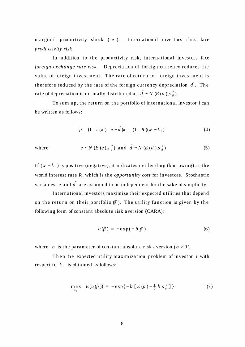
To sum up, the return on the portfolio of international investor i can
be written as follows:
(1 ( ) ) (1 )( )i ir k d k R w kπ ε= + + − + + −%% (4)
where 2 2 ~ ( ( ), ) and ~ ( ( ), )dN E d N E dεε ε σ σ% (5)
If ( iw k− ) is positive (negative), it indicates net lending (borrowing) at the
world interest rate R, which is the opportunity cost for investors. Stochastic
variables and dε % are assumed to be independent for the sake of simplicity.
International investors maximize their expected utilities that depend
on the return on their portfolio (π% ). The utility function is given by the
following form of constant absolute risk aversion (CARA):
( ) exp( )u π β π= − −% % (6)
where β is the parameter of constant absolute risk aversion (β > 0 ).
Then the expected utility maximization problem of investor i with
respect to ik is obtained as follows:
212max ( ( )) exp{ [ ( ) ] }
ikE u E ππ β π β σ= − − −% % (7)

9
where the equality is established by the calculation method that one uses to
find the moment generating function for the normal distribution.
The above expected utility maximization problem is equivalent to the
following maximization problem:
2212max ( , ) ( 1 ( ) ( ) ( ) ) (1 )( )
ii i i i
kk k r k E E d k R w k kφ ε β σ= + + − + + − − (8)
where 2 2 2dεσ σ σ≡ + . This involves only the means and variances of
stochastic variables.
The first order condition for maximization is obtained as follows:
2 2
( ) ( ) ( )( )i
d
r k E E d Rk
ε
εβ σ σ
+ − −=
+ (9)
This gives the optimal action (ki) of investor i as a function of the average
action (k) of other investors. It is the best response function of ki with
respect to k. The second order condition is satisfied because 2 2( ) 0dεβ σ σ+ > .
The optimal portfolio solution clearly shows a tradeoff between risk
and return. The numerator expresses the expected excess rate of return
over the risk free assets while the denominator expresses the risk factors
associated with investing in a foreign country. The optimal investment level
ki is increasing with respect to the return in the numerator and decreasing
with respect to the risk in the denominator. There is a clear tradeoff
between risk and return in the optimal portfolio decision.
C. Strategic complementarity and multiple Nash equilibria
We define strategic complementarity and strategic substitutability in
terms of the function 12( , )ik kφ . International investors face the situation of

10
strategic complementarity if 12( , ) 0ik kφ > . It means that the optimal
investment of an investor increases if other investors increase their
investment. It induces rational herd behavior among international investors.
Conversely, investors face the situation of strategic substitutability if
12( , ) 0ik kφ < . It means that the optimal investment of an investor decreases
if other investors increase their investment. 6 Therefore, strategic
substitutability makes capital flows stable while strategic complementarity
makes capital flows unstable.
In the model, strategic complementarity exists 12( 0)φ > if and only if
the production function exhibits increasing returns to capital ( ( ) 0)f k′′ > .
This proposition follows directly from the fact that
12( , ) ( ) ( )ik k r k f kφ ′ ′′= = (10)
Therefore, strategic complementarity exists in the early stage of development
with increasing returns while strategic substitutability exists in the later
stage of development with decreasing returns. It follows that capital flows
are unstable in the early stage of development while they become stable in
the later stage of development.
Strategic complementarity among the optimal portfolio decisions of
international investors produces multiple Nash equilibria: a low capital
equilibrium and a high capital equilibrium. Figure 5 shows the response
functions of investor i and j ( i j≠ ): that is, the response function of ki with
respect to k which includes kj and the response function of kj with respect to k
which includes ki. Nash equilibria are obtained at the intersection of those
response functions. The Nash equilibria satisfy the condition that
i jk k k= = for all i and j.
6 Cooper and John (1988) and Cooper (1999) discuss the concept of strategic complementarity and strategic substitutability. Strategic complementarity is often associated with multiple equilibria and multiplier effects.

11
There are generally two stable Nash equilibria at Hk and Lk as well
as one unstable Nash equilibrium at Tk , which is located between the two
stable Nash equilibria (Figure 5). Both high and low capital equilibria are
stable Nash equilibria because an investor i has no incentive to deviate from
i Hk k= if other investors choose Hk k= and also from i Lk k= if other
investors choose Lk k= . Although there is another equilibrium ( Tk )
between Lk and Hk , it turns out to be unstable. A small perturbation will
trip the unstable Nash equilibrium ( Tk ), and the economy will move to either
Hk or Lk .7 In other words, the unstable Nash equilibrium ( Tk ) represents
the threshold level of capital.
The two stable Nash equilibria are Pareto-ranked. This follows
directly from the relationship that
2 2 212( , ) ( , ) { ( ) ( ) } 0H H L L H Lk k k k k kφ φ β σ− = − > (11)
It shows that the high capital equilibrium ( Hk ) is a Pareto-superior Nash
equilibrium while the low capital equilibrium ( Lk ) is a Pareto-inferior Nash
equilibrium. All investors prefer the high capital equilibrium to the low
capital equilibrium. The Pareto-ranked multiple equilibria suggest a
possibility of coordination failure that the economy gets stuck at a
Pareto-inferior equilibrium.
If the return factors ( ( ) ( )E E d Rε − − ) are sufficiently large or the
risk factors ( 2 2( )dεβ σ σ+ ) are sufficiently small, the high capital equilibrium
will exist. However, if the return factors are sufficiently small or the risk
factors are sufficiently large, the high capital equilibrium does not exist and
the low capital equilibrium becomes a unique equilibrium (Figure 6).
7 A similar dynamic process may be obtained from a modified neoclassical growth model. For example, equation (9) suggest the following capital flow equation: 2( ) ( ) ( ) ( )dk dt k r k E E d R kε βσ= + − − − . It produces a dynamic process with multiple equilibria, which is analogous to the adjustment process of my model. I owe this point to Delano Villanueva.
12
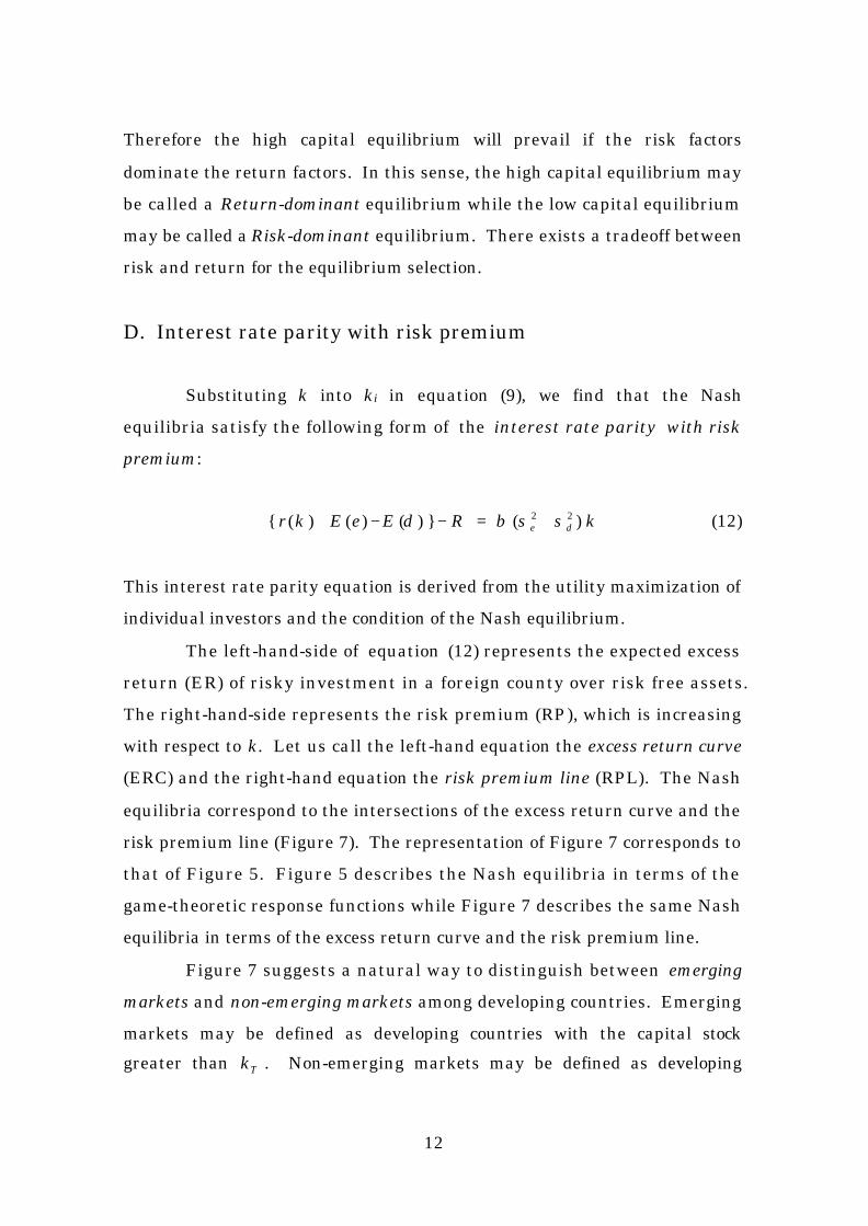
Therefore the high capital equilibrium will prevail if the risk factors
dominate the return factors. In this sense, the high capital equilibrium may
be called a Return-dominant equilibrium while the low capital equilibrium
may be called a Risk-dominant equilibrium. There exists a tradeoff between
risk and return for the equilibrium selection.
D. Interest rate parity with risk premium
Substituting k into ki in equation (9), we find that the Nash
equilibria satisfy the following form of the interest rate parity with risk
premium:
2 2{ ( ) ( ) ( ) } ( )dr k E E d R kεε β σ σ+ − − = + (12)
This interest rate parity equation is derived from the utility maximization of
individual investors and the condition of the Nash equilibrium.
The left-hand-side of equation (12) represents the expected excess
return (ER) of risky investment in a foreign county over risk free assets.
The right-hand-side represents the risk premium (RP), which is increasing
with respect to k. Let us call the left-hand equation the excess return curve
(ERC) and the right-hand equation the risk premium line (RPL). The Nash
equilibria correspond to the intersections of the excess return curve and the
risk premium line (Figure 7). The representation of Figure 7 corresponds to
that of Figure 5. Figure 5 describes the Nash equilibria in terms of the
game-theoretic response functions while Figure 7 describes the same Nash
equilibria in terms of the excess return curve and the risk premium line.
Figure 7 suggests a natural way to distinguish between emerging
markets and non-emerging markets among developing countries. Emerging
markets may be defined as developing countries with the capital stock
greater than Tk . Non-emerging markets may be defined as developing

13
countries with the capital stock less than Tk . Emerging markets are those
countries that converge to the high capital equilibrium ( Hk ) while
non-emerging markets are those that converge to the low capital equilibrium
( Lk ). Developed countries may be defined as those countries that have
already achieved a high level of capital accumulation ( HHk k>> ) where
diminishing returns dominate.
III. Comparative Statics of Return and Risk Factors
This section studies the comparative static properties of the high and
low capital equilibrium with respect to the return and risk factors.
A. Expected exchange rate, expected productivity, and the world
interest rate
The return factors in the model are expected exchange rate ( ( )E d ),
expected productivity ( ( )E ε ), and the world interest rate (R ). Expected
currency depreciation shifts the excess return curve downward by its
magnitude (Figure 8). Expected currency depreciation therefore reduces the
equilibrium capital stock, inducing capital outflows. Conversely, expected
currency appreciation shifts the excess return curve upward by its magnitude.
Expected currency appreciation therefore increases the equilibrium capital
stock, inducing capital inflows.
Those results are confirmed by the following derivative at
,H Lk k k= :
2 2
10
( ) ( ) ( )d
dkdE d f k εβ σ σ
= <′′ − +
(13)
At ,H Lk k k= , the slope of the risk premium line is larger than the slope of

14
the excess return curve: that is, 2 2( ) ( )d f kεβ σ σ ′′+ > . This makes the sign of
the denominator strictly negative.
Similarly, expected productivity increase shifts the excess return
curve upward by its magnitude. It increases the equilibrium capital stock,
inducing capital inflows. Expected productivity decline, on the other hand,
reduces the equilibrium capital stock, inducing capital outflows. A fall in the
world interest rate shifts the excess return curve upward by its magnitude.
It increases the equilibrium capital stock, inducing capital inflows. A rise in
the world interest rate, on the other hand, reduces the equilibrium capital
stock, inducing capital outflows.
These results are confirmed by the following derivatives at
,H Lk k k= :
2 2
10
( ) ( ) ( )d
dkdE f k εε β σ σ
−= >
′′ − + (14)
2 2
10
( ) ( )d
dkdR f k εβ σ σ
= <′′ − +
(15)
Again the sign of the denominator is strictly negative.
B. Exchange rate risk, productivity risk, and risk aversion
The risk factors in the model are the exchange rate risk ( 2dσ ), the
productivity risk ( 2εσ ), and the risk aversion (β ) of international investors.
Increases in those risk factors rotate the risk premium line counter-clockwise.
They reduce the equilibrium capital stock, inducing capital outflows (Figure
9). Decreases in the risk factors, on the other hand, rotate the risk premium
line clockwise. They increase the equilibrium capital stock, inducing capital
inflows. In short, increased risks reduce the equilibrium capital stock,
inducing capital outflows while reduced risks increase the equilibrium capital

15
stock, inducing capital inflows.
These results are confirmed by the following derivative at
,H Lk k k= :
2 2 2 2 0[ ( )] ( ) ( )d d
dk kd f kε εβ σ σ β σ σ
= <′′+ − +
(16)
Again the sign of the denominator is strictly negative.
IV. Mechanism of Economic Takeoff and Capital Flight
This section studies the mechanism of switching between two
equilibria or the mechanism of economic takeoff and capital flight in modern
economic development.
A. Sudden capital inflows and outflows
The comparative static analyses in the previous section have revealed
that the absolute values of derivatives become greater as the level of capital
(k) moves closer to the high critical level ( CHk ) from above (Figure 8 and 9).
This is because the slope of the excess return curve ( )f k′′ increases as k
moves down to CHk from above, decreasing the absolute value of the
denominator and therefore increasing the absolute values of derivatives. In
other words, the effect of a change in the basic factors is greater for the
economy that is located closer to the high critical level of capital ( CHk ). It
goes to infinity as the economy moves onto the high critical level ( CHk ). This
corresponds to the moment of capital flight.
Likewise, the absolute values of derivatives become greater as the
level of capital (k) moves closer to the low critical level ( CLk ) from below
(Figure 8 and 9). This is because the slope of the excess return curve ( )f k′′

16
increases as k moves up to CLk from below, decreasing the absolute value of
the denominator and therefore increasing the absolute values of derivatives.
In other words, the effect of a change in the basic factors is greater for the
economy that is located closer to the low critical level of capital ( CLk ). It
goes to infinity as the economy moves up to the low critical level ( CLk ). This
corresponds to the moment of economic takeoff.
The high capital equilibrium will suddenly disappear if the risk
factors overtake the return factors, bringing the economy below the high
critical level ( CHk ). If the risk premium line and the excess return curve no
longer intersect at Hk , capital outflows will suddenly occur. Conversely,
the low capital equilibrium will suddenly disappear if the return factors
overtake the risk factors, bringing the economy above the low critical level
( CLk ). If the excess return curve and the risk premium line no longer
intersect at Lk , capital inflows will suddenly emerge.
Suppose the economy is initially at H CHk k k= > . Then expected
currency depreciation will reduce the equilibrium level of capital and trigger
capital flight when the excess return curve falls below ER(CH) (Figure 8).
Then the economy will move from H CHk k= to Lk , inducing capital outflows.
This represents capital flight. A similar situation will arise with expected
productivity decline and a fall in the world interest rate.
In addition, a rise in productivity risk and exchange rate risk as well
as the risk aversion of international investors reduces the equilibrium level of
capital. They will trigger capital flight when the risk premium line rotates
counter-clockwise beyond RP(CH) (Figure 9). The economy will move from
H CHk k= to Lk with sudden capital outflows.
In contrast, expected currency appreciation, expected productivity
increase, a fall in the world interest rate, as well as decreases in productivity
risk, exchange rate risk, and the risk aversion of investors create an
environment conducive to achieving economic takeoff with large capital
inflows. They shift the excess return curve upward and rotate the risk

17
premium line clockwise (Figure 8 and 9). The economy will move from
L CLk k= to Hk with the disappearance of the low capital equilibrium.
This represents a takeoff with large capital inflows.
B. Emerging economies and capital flight
The globalization of capital markets is associated with growth in the
number of international investors. An increase in the number of investors
implies an equi-proportionate shift of the excess return curve to the left from
a viewpoint of international investors (Figure 10). In other words, the
amount of foreign investment per investor declines to finance a given amount
of total investment in a developing country. It means enhanced risk-sharing
among investors and reduced risk for each investor. It helps trigger a
takeoff into development. Thus the globalization of capital markets helps
achieve the transformation of developing countries into emerging economies.
Emerging economies ( CHk k> ) are more likely to face capital flight
than developed countries (k k>> ). The minimum shift in the risk premium
line or the excess return curve that can trigger capital flight in a developing
country cannot cause capital flight in a developed country (Figure 7). Only
larger shifts can trigger capital flight in developed countries. This is
because developed countries are operating their production at the level of
diminishing returns and are located further away from the high critical level
of capital ( CHk ).
The emerging economies that are located near the high critical level
are susceptible to capital flight. Those marginal emerging economies
( H CHk k≈ ) exist if international capital markets are efficient and the number
of emerging economies is large. To see this point, suppose there is an
increasing number of emerging economies in the efficient global capital
market. Then, their increasing demand for international capital will induce
the world interest rate to go up until some of the emerging economies are

18
attacked by capital flight. A rise in the world interest rate shifts the excess
return curve down until the supply and demand for international capital in
developing countries are balanced. Therefore there are many emerging
economies near the high critical level of capital ( CHk ). In short, a
combination of an efficient global capital market and a large number of
emerging economies make capital flight more likely to occur. A slight
perturbation of the basic factors can trigger capital flight in marginal
emerging economies.
The crisis of capital flight in one country will increase the perceived
risks ( 2σ ) for investing in other developing countries. The increased risks
can trigger capital flight in other emerging markets (Figure 9). Moreover,
an increasing number of crises will have adverse effects on the risk aversion
of investors ( β ). Like increased risks, a rise in the risk aversion of investors
can trigger capital flight. Therefore the crisis contagion of capital flight can
spread among emerging economies through the increased risks as well as the
increased risk aversion of international investors.
C. Economic takeoff and coordination failure
The existence of the high capital equilibrium is a necessary condition
for capital inflows and economic development. Is it also a sufficient
condition? The answer is no. When there exist multiple equilibria, the
high capital equilibrium is not necessarily selected over the low capital
equilibrium. In other words, coordination failures can arise. The reason for
coordination failures in the model is the stability of both high and low capital
equilibria. History matters and the phenomenon of hysteresis can arise.
Suppose that the economy is initially located at the unique low capital
equilibrium LLk (Figure 7). Now suppose that changes in the return and
risk factors bring the excess return curve and the risk premium line into
intersecting three times at Lk , Tk and Hk . Will the economy move from

19
the low capital equilibrium to the high capital equilibrium? In general, it
will not move so long as the low capital equilibrium continues to exist. This
is because the low capital equilibrium is stable. The economy will stay at
the low capital equilibrium even if the high capital equilibrium exists.
There are two ways in which a developing country can achieve
economic takeoff in this situation. First, the simplest case is that the
expected excess return increases and the risks decline so that the excess
return curve and the risk premium line intersect at the unique high capital
equilibrium HHk (Figure 7). If this happens, the economy will start
economic takeoff with large capital inflows until it converges to the high
capital equilibrium ( HHk ). Second, if international investors can coordinate
their investments so that they invest in a developing country at the same
time above the threshold level ( Tk ). This possibility seems, however, to be
small because of difficulties and costs associated with coordinating a large
number of international investors in a decentralized global capital market in
a way that is compatible with their individual incentives.8
V. Policy Implications
This section studies the policy implications of the model. We have
seen in the previous sections how autonomous changes in the return and risk
factors can bring about economic takeoff and capital flight. To the extent
that the government can control those return and risk factors, it can
influence the equilibrium selection of the economy. Therefore the
developmental role of government can be well defined: It is to help achieve
8 In the above argument, I am assuming that adjustment costs are large so that history dominates expectations in the selection of the final equilibrium. In the presence of large adjustment costs, history determines the equilibrium. Expectations can be important if adjustment costs are small. See Krugman (1991) for the discussion of history versus expectations in the presence of multiple equilibria.

20
the high capital equilibrium through policies that can affect the return and
risk factors in the right directions. What are those policies?
With respect to exchange rate policy, a fixed exchange rate creates an
economic environment conducive to large capital inflows and therefore
economic development. It reduces the exchange rate risk ( 2dσ ) and thus
helps achieve the high capital equilibrium with capital inflows (Figure 9).
This seems to be the main reason why many developing countries have
pegged their local currencies to the currency of international investors. In
contrast, a flexible exchange rate increases the exchange rate risk, and
makes it difficult for a developing country to attract international capital.
As the economy matures into a more advanced stage that is located away
from the critical level ( CHk ) and thus faces less risk of capital flight, the
government can adopt a more flexible exchange rate.9
Suppose that fixed exchange rate policy lost credibility and expected
currency depreciation has triggered capital flight. In other words, the excess
return curve has shifted from ER to below ER(CH) in Figure 8. In this case,
the role of government is to bring the high capital equilibrium back into
existence. This goal can be achieved, for example, if the government
devalues the currency immediately and sufficiently so that investors expect
future appreciation instead of depreciation. It will shift the excess return
curve back to ER and beyond, restoring the high capital equilibrium.
As long as the initial fall in capital is small and capital remains close
enough to the high critical level ( CHk ), an immediate and sufficient
9 The importance of a stable exchange rate for development suggests an answer to the open economy “policy trilemma.” It is well known that the government cannot simultaneously maintain the following three policy goals: (1) free international capital flows , (2) an exchange rate target, and (3) a monetary target. The above discussion about the exchange rate policy suggests that developing countries should seek the (1) and (2) policy goals, while developed countries should seek the (1) and (3) policy goals. The reason is that exchange rate stability is more important for developing countries because they are located closer to the high critical level of capital and therefore susceptible to capital flight.

21
devaluation will bring the economy back to the high capital equilibrium even
though the new equilibrium may be less than the previous level. It will stop
capital flight because the high capital equilibrium is stable. The economy
will move back to the high capital equilibrium so long as it stays near the
equilibrium.10
When combined with the immediate and sufficient devaluation,
capital controls can play an important role in stopping capital flight. If
capital controls can limit capital outflows to a minimum amount, the economy
will return to the high capital equilibrium as soon as the devaluation brings
the equilibrium back into existence. This is because the high capital
equilibrium is stable (Figure 7). Capital controls can also prevent the
economy from moving to the low capital equilibrium by increasing the costs of
capital movements for international investors.11 However, capital controls
can be effective only if they are combined with other policies that help bring
the high capital equilibrium back into existence. Without the re-emergence
of the high capital equilibrium, capital controls will not be able to stop capital
flight because the low capital equilibrium becomes the only equilibrium.
Therefore, the appropriate policy response to capital flight is firstly to limit
the amount of capital outflows, and secondly to bring the high capital
equilibrium back into existence. Capital controls can accomplish the first
objective while the immediate and sufficient devaluation can accomplish the
second objective.
10 In fact, the Asian countries hit by currency crises in 1997 began to recover with the sufficient devaluation that occurred after they gave up their initial attempts to defend currencies. The model suggests that the Asian crisis could have been stopped much earlier and therefore would have been less severe if they had devalued currencies immediately. Devaluation, however, has a negative side-effect that it weakens the balance-sheet of firms with dollar-denominated debts (cf., Krugman (1999)). 11 In the presence of large adjustment costs, history dominates expectations in the selection of the final equilibrium (cf., Krugman (1991)). Therefore, capital controls make it less likely for the economy to shift to the low capital equilibrium as long as the high capital equilibrium exists.

22
Government guarantee for foreign debts can be an effective means to
achieve the high capital equilibrium. From the viewpoint of international
investors, government guarantee is equivalent to purchasing a put option
with the option fee paid by taxpayers. A put option transforms the payoff
function into a convex shape. It has the same effect as an increase in the
expected marginal product ( )E ε and a reduction in the productivity risk 2εσ .
It shifts the excess return curve upward and rotates the risk premium line
clockwise. Therefore, government guarantee increases the probability that
the economy will achieve economic takeoff (Figure 8 and 9).12
The model suggests the two-stage development strategy of domestic
capital accumulation and capital market liberalization. The accumulation of
domestic capital has the effect of shifting the risk premium line to the right
by that amount (Figure 11). Therefore the following two-stage development
strategy becomes an effective means of achieving the high capital
equilibrium: In the first stage, domestic capital ( Dk ) should be accumulated
sufficiently above the level of DCk . In the second stage, capital market
liberalization should be implemented. Then, as Figure 11 shows, the high
capital equilibrium ( Hk ) becomes a unique Nash equilibrium and the optimal
response of international investors is to increase their investment in the
developing country. The country will thus achieve economic takeoff through
the autonomous inflows of international capital ( H Dk k− ).
The capital market liberalization should be implemented only after a
sufficient accumulation of domestic capital is achieved. There are two
12 Moral hazard models argue that government guarantee causes crises because it brings excessively large capital inflows that are to be followed by capital flight (cf., Dooley (2000)). However, a developing country trapped in the low capital equilibrium is suffering from excessively small capital inflows. The purpose of government guarantee is to help the economy shift from the low to the high capital equilibrium by encouraging capital inflows. Government guarantee may result in excessively large capital inflows if it continues to exist even after the economy has achieved the high capital equilibrium.

23
reasons: First, capital market liberalization will not help the economy to
achieve the high capital equilibrium if domestic capital is less than DCk .
Second, capital market liberalization will bring about some outflows of
domestic capital. Therefore, it becomes necessary for achieving the high
capital equilibrium that domestic capital ( Dk ) remains above the critical level
( DCk ) after some outflows of domestic capital due to the liberalization.
Otherwise the country will be trapped in the low capital equilibrium.
The role of government must change with the stages of economic
development. During the stage of increasing returns and complementarity ,
the government can help achieve the high capital equilibrium through
policies that affect the return and risk factors in the right directions.
However, after the high capital equilibrium is achieved and the risk of capital
flight is reduced, the role of government must change. Those interventional
policies become distortionary for the economy that is characterized by
decreasing returns and substitutability . Therefore, they must be abolished
after the economy has achieved a successful takeoff.
VI. Conclusion
I have presented a model of economic takeoff and capital flight with
free international capital flows. In the early stage of development,
investments are complementary and aggregate production exhibits increasing
returns to capital. The increasing returns lead to strategic complementarity
between the optimal portfolio decisions of international investors. The
result is multiple Nash equilibria: a high capital equilibrium and a low
capital equilibrium. The model has shown how changes in the return and
risk factors can trigger switches between two equilibria. Switches between
two equilibria correspond to the economic takeoff and capital flight of a
developing country.
At the high capital equilibrium, the interest rate parity with risk

24
premium holds and international capital allocation is efficient. If the risk
factors dominate the return factors, the high capital equilibrium will
disappear. Then, capital flight becomes inevitable. Conversely, if the
return factors dominate the risk factors, the low capital equilibrium will
disappear. Then, autonomous capital inflows will bring about the economic
takeoff of the developing country.
To the extent that the government can influence the return and risk
factors, it can affect the selection of the equilibrium in the economy.
Therefore the role of government is to help achieve the high capital
equilibrium through policies that affect the return and risk factors. Fixed
exchange rate policy, government guarantee, and capital control potentially
help achieve the high capital equilibrium. However, after the economy is
sufficiently developed to the level of decreasing returns, those policies become
distortionary and therefore should be abolished.
The globalization of capital markets helps achieve the high capital
equilibrium through risk-sharing among the increasing number of investors.
The two-stage development strategy of domestic capital accumulation and
capital market liberalization can also help achieve the high capital
equilibrium. It enables the economy to achieve economic takeoff with
autonomous capital inflows from the global capital market. However, the
economy may be trapped in the low capital equilibrium if the liberalization is
implemented before the sufficient accumulation of domestic capital.
25
References
Ades, A. and E. Glaeser (1999): “Evidence on Growth, Increasing Returns,
and the Extent of the Market,” Quarterly Journal of Economics (114):
1025-45.
Aoki, M., H-K. Kim, and M. Okuno-Fujiwara (1996): The Role of Government
in East Asian Economic Development, New York: Oxford University
Press.
Baumol, W., S. Batey Blakman, and E. Wolf (1989): Productivity and
American Leadership: The Long View, Cambridge, MA: MIT Press.
Cooper, R. (1999): Coordination Games: Complementarities and
Macroeconomics, Cambridge: Cambridge University Press.
Cooper, R. and A. John (1988): “Coordinating Coordination Failures in
Keynesian Models,” Quarterly Journal of Economics (103): 441-63.
Corsetti, G., P. Pesenti, and N. Roubini (1998): “What Caused the Asian
Currency and Financial Crises?” Unpublished paper.
Dollar, D. (1992): “Exploiting the Advantages of Backwardness: The
Importance of Education and Outward Orientation,” World Bank,
Unpublished paper.
Dooley, M. (2000): “A Model of Crieses in Emerging Markets,” Economic
Journal (110): 256-72.
Easterly, W. (1994): “Economic Stagnation, Fixed Factors, and Policy
Thresholds,” Journal of Monetary Economics (33): 525-57.
Fleming, J. (1955): “External Economies and the Doctrine of Balanced
Growth,” Economic Journal (65): 241-56.
Furman, J. and J. Stiglitz (1998): “Economic Crises: Evidence and Insights
from East Asia,” Brookings Papers on Economic Activity (2): 1-132.
Hirschman, A. (1958): The Strategy of Economic Development, New Haven:
Yale University Press.
Ito, T. (1999): “Capital Flows in Asia,” NBER Working Paper 7134.

26
Ito, T et al. (2000): “East Asian Economic Growth with Structural
Change,” The Keizai Bunseki (The Economic Analysis) (No.160),
Economic Research Institute, Economic Planning Agency.
King, R. and S. Rebelo (1993): “Transitional Dynamics and Economic Growth
in the Neoclassical Model,” American Economic Review (83): 908-31.
Kremer, M. (1993): “The O-Ring Theory of Ecoomic Development,” Quarterly
Journal of Economics (108): 551-75.
Krugman, P. (1991): “History versus Expectatoins,” Quarterly Journal of
Economics (106): 651-67.
Krugman, P. (1999): “Balance sheets, the transfer problem, and financial
crises,” forthcoming in Robert Flood Festschrift volume.
Lewis, A. (1955): The Theory of Economic Growth, London: George Allen &
Unwin Ltd.
Matsuyama, K. (1991): “Increasing Returns, Industrialization, and
Indeterminacy of Equilibrium,” Quarterly Journal of Economics (106):
617-50.
Matsuyama, K. (1992): “The Market Size, Entrepreneurship, and the Big
Push,” Journal of Japanese and International Economies (6): 347-64.
Murphy, K., A. Shleifer, and R. Vishny (1989): “Industrialization and the Big
Push,” Journal of Political Economy (97): 1003-26.
Nurkse, R. (1953): Problems of Capital Formation in Underdeveloped
Countries, New York: Oxford University Press.
Okazaki, T. (1996): “The Government-Firm Relationship in Postwar Japanese
Economic Recovery: Resolving the Coordination Failure by
Coordination in Industrial Rationalization,” in Aoki, Kim, and
Okuno-Fujiwara (1996): 74-100.
Radelet, S. and Jeffrey Sachs (1998): “The Onset of the East Asian Crisis,”
Unpublished paper, Harvard Institute for International Development.
Rosenstein-Rodan, P. (1943): “Problems of Industrialization of Eastern and
South-Eastern Europe,” Economic Journal (53): 202-11.

27
Scitovsky, T. (1954): “Two Concepts of External Economies,” Journal of
Political Economy (62): 143-51.
Singer, H. (1949): “Economic Progress in Underdeveloped Countries,” Social
Research (16): 1-11.
World Bank (1998a): Global Development Finance, Washington D.C.
World Bank (1998b): East Asia: The Road to Recovery, Washington, D.C.
Young, A. (1928): “Increasing Returns and Economic Progress,” Economic
Journal (38): 527-42.

Figure 1 The Conventional Production Function with Decreasing Returns
( )f k k− ( a )
0 k
( ) ( ) 1r k f k′= − ( b )
0
k

Figure 2 Development Stages and Growth Rate (OECD Countries)
0
0.01
0.02
0.03
0.04
0.05
0.06
0.07
0 5,000 10,000 15,000 20,000 25,000
GDP per worker, 1960
Gro
wth
rat
e, 1
960-
90
Source: Penn World Tables, Mark 5.6
Figure 3 Development Stages and Growth Rate (104 Countries)
-0.03
-0.02
-0.01
0
0.01
0.02
0.03
0.04
0.05
0.06
0.07
0 5,000 10,000 15,000 20,000 25,000
GDP per worker, 1960
Gro
wth
rat
e, 1
960-
90
Source: Penn World Tables, Mark 5.6

Figure 4 Production Function with Increasing and Decreasing Returns
( )f k k− ( a )
0 k
k
( ) ( ) 1r k f k′= − ( b )
0
k k

Figure 5 Response Functions and Multiple Nash Equilibria
ik , k
Hk P S NE
Tk
Lk
P I NE
k, kj
Lk Tk Hk
P S NE = Pareto-Superior Nash Equilibrium
PINE = Pareto-Inferior Nash Equilibrium
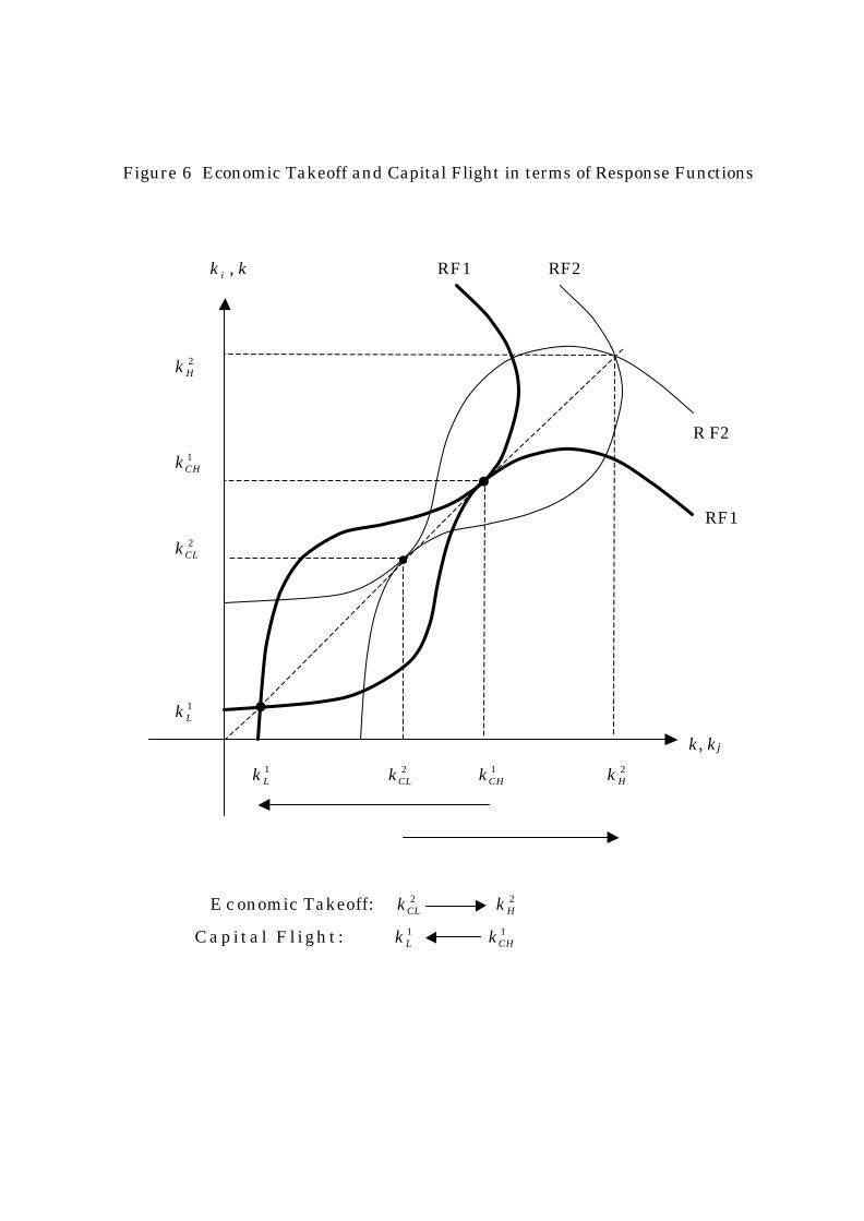
Figure 6 Economic Takeoff and Capital Flight in terms of Response Functions
ik , k RF1 RF2
2Hk
R F2
1CHk
RF1
2CLk
1Lk
k, kj
1Lk 2
CLk 1CHk 2
Hk
E c onomic Takeoff: 2CLk 2
Hk
Capita l Fl ight : 1Lk 1
CHk

Figure 7 Excess Return Curve and Risk Premium Line
ER, RP
RP(LL)
R P = εβ σ σ+2 2( )d k
R P ( H H )
E R = { ( ) ( ) ( )}r k E E d Rε+ − −
k
LLk Lk Tk Hk HHk
Lk Tk Hk
Risk Premium Line: RP = εβ σ σ+2 2( )d k
Excess Return Curve: ER = { ( ) ( ) ( )}r k E E d Rε+ − −

Figure 8 Changes in Expected Exchange Rate, Expected Productivity,
and the World Interest Rate
ER, RP
R P
E R (CL)
E R
E R (CH)
0 k
Lk CLk Tk CHk Hk

Figure 9 Changes in Exchange Rate Risk, Productivity Risk, and Risk Aversion
ER, RP
R P ( C H )
R P
R P (CL)
E R
k
Lk CLk Tk CHk Hk

Figure 10 Globalization of Capital Markets and Economic Takeoff
ER, RP
RP
ER
0 k
Lk CLk Hk

Figure 11 Domestic Capital Accumulation and Capital Market Liberalization
ER, RP
RP
ER
0 k
Lk DCk Dk Hk
Domestic Capital Accumulation = Dk
Capital Inflows = H Dk k−