economic scenarios generators in r with esgtoolkit

EconomicScenarios

Generation forInsurance:

ESGtoolkit (andfriends)

Thierry Moudiki(@moudikithierry)

Economic Scenarios Generation forInsurance: ESGtoolkit (and friends)Institut de Sciences Financières et d’Assurances,

Université Lyon 1

Thierry Moudiki (@moudikithierry)

September 26, 2014

EconomicScenarios




EconomicScenarios




Contents

1. Context2. ESGtoolkit

I About model riskI About discretization errorI About calibration error

EconomicScenarios




Why ?

I As an insurer, basically :I How much should I keep aside today at t = 0, for the

payment of a guaranteed compensation tomorrow att = T :

Liabs0 = BestEstimateLiabs0 + Margin0

=⇒ Reserving : pricing the guaranteed compensationI Having calculated Liabs0, I’d like to derive xα > 0, so

that :

P(AssetsT − LiabsT > xα) ≥ 1− α%

=⇒ Capital modeling : determining the futuredistribution of my Own Funds

EconomicScenarios




Why ? (cont’d)

Regulatory point of view

I Market Consistent Embedded value (MCEV) :Time Value of Financial Options & Guarantees (TVOFG)

I **Solvency II :I ** Best Estimate valuation of the technical reserves

(BEL)I Solvency II : Own Risk Solvency Assessment (ORSA)

But :

I For pricing (reserving) : not always closed formulasavailable for pricing the guarantees (risk asymmetryinduced by the optional features)

I For capital modeling : not always (never !)entirely-specified probability distributions available forthe Own Funds

EconomicScenarios




Context

What ?From what’s been said : Modeling and simulation of riskfactors are needed.

ESG : Economic Scenarios Generator

I Tool for modeling and simulation of economic factors’future values

I Purpose : Asset & Liability Management in Bankingand Insurance.

I Our focus : Insurance

EconomicScenarios




How ?How can we do that ?

I With Monte Carlo simulationI But also, Bootstrapping can be used

Generally, 2 types of simulations

I Real-world simulations under the objective probability :for capital modeling

I Risk-neutral simulations under a martingale probabilitymeasure : for reserving/pricing

EconomicScenarios



Thierry Moudiki(@moudikithierry)The package ESGtoolkit

I An R package providing tools, for constructing customEconomic Scenario Generators (ESG)

I Version 0.1 released in june 2014I A vignette is available (now in PDF, in HTML soon)I Under developmentI Suggestions, bug reports, and features request are

welcome.

http://cran.r-project.org/web/packages/ESGtoolkit/vignettes/ESG2toolkit_Intro_062014.pdf

EconomicScenarios




Why R ?

I The language of Analytics; 2 million users worldwide(Source : Seven quick facts about R)

I Free + Open sourceI Over 5800 contributed packages on CRAN repository,

doing almost anything you could think of (Visit : theTask Views)

I “Researchers in statistics and machine learning willoften publish an R package to accompany theirarticles. This means immediate access to the verylatest statistical techniques and implementations.”Hadley Wickham (RStudio)

http://blog.revolutionanalytics.com/2014/04/seven-quick-facts-about-r.html

http://cran.r-project.org/web/views/

http://cran.r-project.org/web/views/

http://adv-r.had.co.nz/Introduction.html

EconomicScenarios




Contents



EconomicScenarios




ESGtoolkitI Currently, 3 main functions

I simdiff (underlying C++ code via Rcpp) :I Ornstein-Uhlenbeck process simulationI Cox-Ingersoll-Ross process simulationI Geometric Brownian motion with constant or

time-dependent drift or volatility, and optional(lognormal or double-exponential) jumps

I simshocks :I simulation of gaussian shocks with highly flexible

dependence structureI esgfwdrates :

I instantaneous forward rates for no-arbitrage short ratemodels

I And additional functions for diagnostics :esgplotbands, esgplotshocks,esgplotmartingaletest, . . .

http://cran.r-project.org/web/packages/Rcpp/index.html

EconomicScenarios




ESGtoolkitESGtoolkit current structure

esgfwdrates (Nelson−Siegel, Smith−Wilson ...)

simdiff (OU, CIR, GBM−likes)

simshocks (Gaussian, Student t, Clayton ...)

no−arbitrage short rates models (HW, G2++, CIR++, BK, ...)

various models (Vasicek, BS, Merton, Heston, Bates...)

EconomicScenarios




However, remember

I “Essentially, all models are wrong, but some are useful”George E. P. Box

I . . . also, some can lead to disasters.

EconomicScenarios




From Felix Salmon’s Recipe for Disaster: The Formula ThatKilled Wall Street (available online)

http://archive.wired.com/techbiz/it/magazine/17-03/wp_quant?currentPage=all

http://archive.wired.com/techbiz/it/magazine/17-03/wp_quant?currentPage=all

EconomicScenarios




However, remember

3 types of risks in the process of modeling and simulation ofrisk factors :

I Model riskI Choice of the modelI Choice of the dependence structure

I Discretization errorI Calibration error

EconomicScenarios




Contents



EconomicScenarios




About model risk

Choice of the model and choice of the dependencestructureA simple example : Insurance company, ABC corp., thathas, on December 30, 2011, 2 assets in its portfolio :

A0 = Nominal × (40%CAC 40 + 60%S&P 500)

The liabilities on December 30, 2011 are :

L0 = 45%× A0

ABC corp. has to pay daily guaranteed benefits K to theinsured, plus an additional benefits depending on the dailyperformance of the assets :

∀i > 0, Li = Li−1 − K ×(1 + 95%max

( AiAi−1

− 1, 0))

EconomicScenarios




Analyst wants to assess ABC corp.’s 6-month solvencyand uses R

# loading the package quantmod# to obtain financial index time serieslibrary(quantmod)

# Importing the values of the CAC40 and S&P500# CAC40, as a time series (ts) objectgetSymbols('^FCHI', src='yahoo',

return.class = 'ts',from = "2011-06-30",to = "2011-12-30")

# S&P500, as a time series (ts) objectgetSymbols('^GSPC', src='yahoo',

return.class = 'ts',from = "2011-06-27",to = "2011-12-30")

EconomicScenarios




The type of data we can get from quantmod

head(FCHI)[, 1:4]

## FCHI.Open FCHI.High FCHI.Low FCHI.Close## [1,] 3937 3982 3926 3982## [2,] 3982 4024 3967 4007## [3,] 4010 4010 3997 4003## [4,] 3997 3999 3974 3979## [5,] 3981 3982 3942 3961## [6,] 3982 4020 3960 3980

EconomicScenarios



Thierry Moudiki(@moudikithierry)I Using the closing prices S(CAC)

t , S(SP)t analyst calculates

the daily log-returns

log

S(CAC)ti+1

S(CAC)ti

and

log

S(SP)ti+1

S(SP)ti

EconomicScenarios




Normality of the log-returns ?Histogram of log.ret.CAC

log.ret.CAC

Fre

quen

cy

−0.06 −0.04 −0.02 0.00 0.02 0.04 0.06

05

1015

2025

−2 −1 0 1 2

−0.

06−

0.02

0.02

0.06

Normal Q−Q Plot

Theoretical Quantiles

Sam

ple

Qua

ntile

s

Histogram of log.ret.SP

log.ret.SP

Fre

quen

cy

−0.06 −0.04 −0.02 0.00 0.02 0.04

05

1015

2025

30

−2 −1 0 1 2

−0.

06−

0.02

0.02

Normal Q−Q Plot

Theoretical Quantiles

Sam

ple

Qua

ntile

s

EconomicScenarios




Normality of the log-returns ? (cont’d)

shapiro.test(log.ret.CAC)

#### Shapiro-Wilk normality test#### data: log.ret.CAC## W = 0.9906, p-value = 0.5268

shapiro.test(log.ret.SP)

#### Shapiro-Wilk normality test#### data: log.ret.SP## W = 0.9827, p-value = 0.0962

EconomicScenarios




Maximum likelihood estimation

I Analyst assumes that :I the distribution of the assets over the next 6months will be the same that she observed in thelast 6-months period.

Maximum likelihood is used to calibrate the lognormalmodels :

# Parameters for the projection of the CAC 40delta <- 1/252 # for daily samplingsigma.CAC <- sqrt((n-1)/n)*sd(log.ret.CAC)/sqrt(delta)mu.CAC <- mean(log.ret.CAC)/delta +

0.5*sigma.CAC^2

EconomicScenarios




Correlation ?

I Based on :I the histogramsI the Normal qqplotI the results of the tests (Normality not rejected)

ABC corp.’s analyst assumes that the distribution of theassets on the period of interest is lognormal.

I But she now wants to know more about thedependence between the assets

EconomicScenarios




Correlation ? (cont’d)

I Visualizing the indices on the 6-month period, and thelog-returns

CAC 40

Time

S.C

AC

0 20 40 60 80 100 120

2800

3400

4000

S&P 500

Time

S.S

P

0 20 40 60 80 100 120

1100

1200

1300

0 20 40 60 80 100 120

−0.

060.

000.

04

log−returns

Index

log.

ret.C

AC

EconomicScenarios





I She decides toI assume that the assets are correlated (Gaussiandependence).

The correlation coefficients between the shocks is :

U.S.CAC <- pnorm((log.ret.CAC - mean(log.ret.CAC))/sd(log.ret.CAC))

U.S.SP <- pnorm((log.ret.SP - mean(log.ret.SP))/sd(log.ret.SP))

(correlation <- cor(U.S.CAC, U.S.SP))

## [1] 0.3852

EconomicScenarios





However. . .

# Package CDVine : Statistical inference of# canonical vine (C-vine) and D-vine copulaslibrary(CDVine)copula.selection <- BiCopSelect(U.S.CAC, U.S.SP)print(c(copula.selection$family, copula.selection$par,

copula.selection$par2))

## [1] 2.0000 0.4227 9.1056

I R package CDVine (see jstatsoft paper) says :I Student t dependence, with 9.11 degrees of freedom,

and dependence parameter equal to 0.42

http://www.jstatsoft.org/v52/i03/paper

EconomicScenarios




I Simulation of shocks with ESGtoolkit

library(ESGtoolkit)# Nb of simulations, horizon, and frequencynb <- 10000horizon <- 1freq <- "daily"# Simulation of shocksset.seed(1)# With student dependenceeps.student <- simshocks(n = nb,horizon = horizon, frequency = freq,family = copula.selection$family,par = copula.selection$par,par2 = copula.selection$par2)

EconomicScenarios




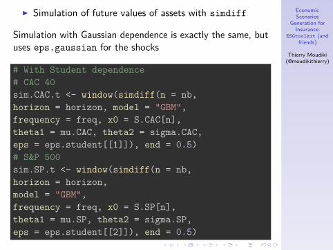
I Simulation of future values of assets with simdiff

Simulation with Gaussian dependence is exactly the same, butuses eps.gaussian for the shocks

# With Student dependence# CAC 40sim.CAC.t <- window(simdiff(n = nb,horizon = horizon, model = "GBM",frequency = freq, x0 = S.CAC[n],theta1 = mu.CAC, theta2 = sigma.CAC,eps = eps.student[[1]]), end = 0.5)# S&P 500sim.SP.t <- window(simdiff(n = nb,horizon = horizon,model = "GBM",frequency = freq, x0 = S.SP[n],theta1 = mu.SP, theta2 = sigma.SP,eps = eps.student[[2]]), end = 0.5)

EconomicScenarios




I Visualizing the projections of assets’ values withesgplotbands

par(mfrow = c(2, 2))esgplotbands(sim.CAC.t, xlab = "time",

ylab = "index values")lines(S.CAC.future, col = "red")esgplotbands(sim.SP.t, xlab = "time",

ylab = "index values")lines(S.SP.future, col = "blue")esgplotbands(sim.CAC.g, xlab = "time",

ylab = "index values")lines(S.CAC.future, col = "red")esgplotbands(sim.SP.g, xlab = "time",

ylab = "index values")lines(S.SP.future, col = "blue")

EconomicScenarios




I Visualizing the projections of assets’ values withesgplotbands. The true values (from January to June2012) are the red lines and the blue lines.

0.0 0.1 0.2 0.3 0.4 0.5

1000

2000

3000

4000

5000

6000

7000

8000

CAC 40 projection (Student dependence)

time

inde

x va

lues

0.0 0.1 0.2 0.3 0.4 0.5

500

1000

1500

2000

2500

S&P 500 projection (Student dependence)

time

inde

x va

lues

0.0 0.1 0.2 0.3 0.4 0.5

1000

2000

3000

4000

5000

6000

7000

CAC 40 projection (gaussian dependence)

time

inde

x va

lues

0.0 0.1 0.2 0.3 0.4 0.5

500

1000

1500

2000

2500

3000

S&P 500 projection (gaussian dependence)

time

inde

x va

lues

EconomicScenarios




I Assets and Liabilities simulation for the Net Asset Value(the whole code is available)

### The insurer's Assetw1 <- 0.4w2 <- 1-w1Nominal <- 100000# With gaussian dependenceS.g <- Nominal*(w1*sim.CAC.g + w2*sim.SP.g)# With Student t dependenceS.t <- Nominal*(w1*sim.CAC.t + w2*sim.SP.t)

### The insurer's liability# With gaussian and Student t dependence (at t=0)L0.g <- L0.t <- S.g[1,1]*0.45# Guaranteed capitalK <- 80# Pct. for additional benefitspct.PB <- .95

EconomicScenarios




I Assets and Liabilities simulation for the Net Asset Value

# variation of liabilitiesfact.growth.t <- -K*(1 + pct.PB*(S.t.mat[-1, ]/

S.t.mat[-nrowS, ] - 1)*(S.t.mat[-1, ]/S.t.mat[-nrowS, ] - 1 > 0))

# Liabilities simulation (Student)L.t <- ts(apply(rbind(rep(L0.t, ncolS), fact.growth.t), 2,

cumsum),start = start(S.t), deltat = deltat(S.t))

# Net Asset ValueNAV.t <- S.t - L.t

EconomicScenarios




I Estimating the 6-month required capital with Gaussianand Student dependences (the whole code is available)

# VaR Gaussian vs Student dep.qt.NAV.t <- quantile(NAV.t.last,

probs = 1 - c(0.9, 0.95, 0.995))(qt.NAV.t/qt.NAV.g - 1)*100

## 10% 5% 0.5%## -1.9779 -1.4868 -0.4514

# TVaR Gaussian vs Student dep.TVaR.NAV.t <- mean(sort(NAV.t.last)[1:50])(TVaR.NAV.t/TVaR.NAV.g - 1)*100

## [1] -5.767

EconomicScenarios




But still. . .

I Historical stock prices are NOT lognormal.I Even though it’s based on real data, this was a “nice”

example.I Try other models : Heston model (stochastic volatility)

or Bates model (stochastic volatility with jumpsdiffusion)

I Example : The package’s vignette explains how tomake simulations of Bates model

I But :I calibration must be carried out with careI validation of statistical properties as well

http://cran.r-project.org/web/packages/ESGtoolkit/vignettes/ESG2toolkit_Intro_062014.pdf

EconomicScenarios




Contents



EconomicScenarios




About discretization error

I Example

A Stochastic Differential Equation for an equilibrium shortrate model (Vasicek model’s SDE) :

drt = a(θ − rt)dt + σdWt

A simple and intuitive way to make simulations of the SDE :Euler scheme (1st order Ito development) :

I Deterministic mean-reverting part

rti+1 − rti = a(θ − rti )(ti+1 − ti ) + . . .

I . . . A part with random shocks (ε ∼ N (0, 1))

σε√

ti+1 − ti

EconomicScenarios




About discretization error (cont’d)

I Other method for the simulation of SDE : Milsteinscheme (2nd order Ito development). But when e.g thevolatility σ is constant, it’s not necessary. Otherwise,leads to more complicated formulas.

I Euler and Milstein schemes imply discretization bias.I Currently in ESGtoolkit, we use exact simulation of

the transition distribution between ti+1 and ti =⇒ Nodiscretization bias.

Here, using the SDE’s exact solution provides the followingalternative scheme :

rti+1 = e−a(ti+1−ti )rti +θ(1−e−a(ti+1−ti ))+σε

√1− e−a(ti+1−ti )

2a

EconomicScenarios




I Illustration using ESGtoolkit (set.seed(1))

m <- 50 # number of projection datesn <- 500 # number of simulationsa <- 0.5 # speed of mean-reversiontheta <- 0.02 # long term rate, mean-rev. levelsigma <- 0.001 # volatility

# Short rate with Euler discretizationr.Euler <- matrix(0, nrow = m, ncol = n)for (i in 1:(m-1)){r.Euler[i+1, ] <- r.Euler[i, ] + a*(theta -r.Euler[i, ]) + sigma*rnorm(n)}

# Short rate with Exact simulation (ESGtoolkit)r.Exact <- simdiff(n = n, horizon = 50,

model = "OU",x0 = 0, theta1 = a*theta,theta2 = a, theta3 = sigma)

EconomicScenarios




0.012 0.014 0.016 0.018

010

030

050

0

Visualizing discretization bias (t = 3 years) on the example, through densities

N = 500 Bandwidth = 0.0003097

Den

sity

Euler simulationExact simulation (ESGtoolkit)

0.016 0.018 0.020 0.022

010

030

050

0


N = 500 Bandwidth = 0.0002621

Den

sity


0.016 0.018 0.020 0.022 0.024

010

030

050

0


N = 500 Bandwidth = 0.0002712

Den

sity


0.016 0.018 0.020 0.022 0.024

010

030

050

0


N = 500 Bandwidth = 0.000304

Den

sity


EconomicScenarios




About discretization error (cont’d)

I Comparing the implied zero-coupon prices

price.Euler <- rowMeans(exp(-apply(r.Euler, 2,cumsum)))

price.Exact <- rowMeans(exp(-apply(r.Exact, 2,cumsum)))

(head(price.Exact)/head(price.Euler) - 1)*100

## [1] 0.0000 0.2071 0.4452 0.6392 0.7936 0.9002

EconomicScenarios




Contents



EconomicScenarios




Calibration (the Art of)

I Choice of projection models parameters usingmarket data

I Real worldI Methods of moments (Generalized, Simulated)I Maximum likelihood (or Quasi-Maximum likelihood,

Normal approximation, Simulated maximum likelihood)I Non-linear filtering

I Market Consistent (Risk-neutral)I Minimizing (for N given financial instruments)

N∑i=1

wig(Price(i,Model)0 (Θ)− Price(i,Market)

0 )

I With model parameters Θ ∈ Rd , weights (wi )i=1,...,Nand for example :

I g : x 7→ x2

I g : x 7→ |x |

EconomicScenarios




Focus on market consistent calibrationCRO Forum, in Extrapolation of Market Data (2010)

I The complexity of the stochastic model used to valueembedded options and guarantees is directly linked tothe complexity of the underlying insurance contract

I The complexity of the model used should take intoaccount the complexity of the liability and its embeddedequity guarantees [. . . ]. The calibration of any modelshould at least consider the at-the-money term-structureand for more complex models (e.g. Heston) should alsoconsider the full volatility surface of the liquid part of thevolatility market. This then automatically impliesextrapolated volatilities for in- and out-the-moneyvolatilities in the extrapolated part of the curve.

http://www.thecroforum.org/cro-forum_extrapolation-of-market-data/

EconomicScenarios




Focus on market consistent calibration (cont’d)

I Example : G2++ model (2-factor Hull & White)calibrated to ATM Euro Caps on December 31, 2011

dxt = −axt + σdW (x)t

dyt = −byt + ηdW (y)t

dW (x)t dW (y)

t = ρdt

rt = xt + yt + Φt

I 5 parameters to find : a, b, σ, η, ρI Objective function with many local optimaI Optimization with R package mcGlobaloptim

I Monte Carlo simulation of multiple starting points in agiven region

I Running local optimizationsI Finding the best parameters

EconomicScenarios




Focus on market consistent calibration (cont’d)

# Parameters found for the G2++a_opt <- 0.50000000b_opt <- 0.35412030sigma_opt <- 0.09416266rho_opt <- -0.99855687eta_opt <- 0.08439934

horizon <- 20n <- 500freq <- "semi-annual"delta_t <- 1/2

# Simulation of gaussian correlated shockseps <- simshocks(n = n, horizon = horizon,

frequency = freq,method = "anti",family = 1, par = rho_opt)

EconomicScenarios




I Simulation of the model factors

x <- simdiff(n = n, horizon = horizon,frequency = freq,model = "OU",x0 = 0, theta1 = 0, theta2 = a_opt, theta3 = sigma_opt,eps = eps[[1]])

y <- simdiff(n = n, horizon = horizon,frequency = freq,model = "OU",x0 = 0, theta1 = 0, theta2 = b_opt, theta3 = eta_opt,eps = eps[[2]])

EconomicScenarios




I Forward rates and final model

fwdrates <- esgfwdrates(n = n, horizon = horizon,out.frequency = freq, in.maturities = u,in.zerorates = txZC, method = "SW")fwdrates <- window(fwdrates, end = horizon)

t.out <- seq(from = 0, to = horizon,by = delta_t)

param.phi <- 0.5*(sigma_opt^2)*(1 -exp(-a_opt*t.out))^2/(a_opt^2) +0.5*(eta_opt^2)*(1 - exp(-b_opt*t.out))^2/

(b_opt^2) +(rho_opt*sigma_opt*eta_opt)*(1 - exp(-a_opt*t.out))*

(1 - exp(-b_opt*t.out))/(a_opt*b_opt)

EconomicScenarios




I Forward rates and final model (cont’d)

param.phi <- ts(replicate(n, param.phi),start = start(x), deltat = deltat(x))

phi <- fwdrates + param.phicolnames(phi) <- c(paste0("Series ", 1:n))

r <- x + y + phicolnames(r) <- c(paste0("Series ", 1:n))

EconomicScenarios




I The result

esgplotbands(r, xlab = "time", ylab = "values",main = "G2++ short rate")

lines(rep(0, ncol(r)), col = "red", lty = 2, lwd = 2)

0 5 10 15 20

−0.

050.

000.

050.

10

G2++ short rate

time

valu

es

EconomicScenarios




I Monte Carlo prices of zero-coupons vs true prices

5 10 15 20

0.65

0.70

0.75

0.80

0.85

0.90

0.95

1:horizon

win

dow

(esg

mcp

rices

(r, 1

), s

tart

= 0

.5, d

elta

t = 1

)

zero−coupon pricesm.c G2++ zero−coupons

EconomicScenarios




# Checking error manuallypct.err <- (window(esgmcprices(r, 1),start = 0.5, deltat = 1)/p[1:horizon] - 1)*100plot(pct.err)points(pct.err)

Time

pct.e

rr

0 5 10 15 20

−0.

20−

0.15

−0.

10−

0.05

0.00

EconomicScenarios




One further step is required

I Verifying by simulation that the discounted Caps payoffsare martingales (Market consistency test)

I Typically, a Student t-testI An example of Market consistency test can be found

in the package vignette.

economic scenarios generators in r with esgtoolkit

Software