economic restructuring and total factor productivity ... · economic restructuring and total factor...
TRANSCRIPT

Montréal
Juin 2010
© 2010 Sofiane Ghali, Pierre Mohnen. Tous droits réservés. All rights reserved. Reproduction partielle permise
avec citation du document source, incluant la notice ©.
Short sections may be quoted without explicit permission, if full credit, including © notice, is given to the source.
Série Scientifique
Scientific Series
2010s-26
Economic Restructuring and Total Factor Productivity
Growth: Tunisia Over the Period 1983-2001
Sofiane Ghali, Pierre Mohnen

CIRANO
Le CIRANO est un organisme sans but lucratif constitué en vertu de la Loi des compagnies du Québec. Le financement de
son infrastructure et de ses activités de recherche provient des cotisations de ses organisations-membres, d’une subvention
d’infrastructure du Ministère du Développement économique et régional et de la Recherche, de même que des subventions et
mandats obtenus par ses équipes de recherche.
CIRANO is a private non-profit organization incorporated under the Québec Companies Act. Its infrastructure and research
activities are funded through fees paid by member organizations, an infrastructure grant from the Ministère du
Développement économique et régional et de la Recherche, and grants and research mandates obtained by its research
teams.
Les partenaires du CIRANO
Partenaire majeur
Ministère du Développement économique, de l’Innovation et de l’Exportation
Partenaires corporatifs
Banque de développement du Canada
Banque du Canada
Banque Laurentienne du Canada
Banque Nationale du Canada
Banque Royale du Canada
Banque Scotia
Bell Canada
BMO Groupe financier
Caisse de dépôt et placement du Québec
Fédération des caisses Desjardins du Québec
Gaz Métro
Hydro-Québec
Industrie Canada
Investissements PSP
Ministère des Finances du Québec
Power Corporation du Canada
Raymond Chabot Grant Thornton
Rio Tinto
State Street Global Advisors
Transat A.T.
Ville de Montréal
Partenaires universitaires
École Polytechnique de Montréal
HEC Montréal
McGill University
Université Concordia
Université de Montréal
Université de Sherbrooke
Université du Québec
Université du Québec à Montréal
Université Laval
Le CIRANO collabore avec de nombreux centres et chaires de recherche universitaires dont on peut consulter la liste sur son
site web.
ISSN 1198-8177
Les cahiers de la série scientifique (CS) visent à rendre accessibles des résultats de recherche effectuée au CIRANO
afin de susciter échanges et commentaires. Ces cahiers sont écrits dans le style des publications scientifiques. Les idées
et les opinions émises sont sous l’unique responsabilité des auteurs et ne représentent pas nécessairement les positions
du CIRANO ou de ses partenaires.
This paper presents research carried out at CIRANO and aims at encouraging discussion and comment. The
observations and viewpoints expressed are the sole responsibility of the authors. They do not necessarily represent
positions of CIRANO or its partners.
Partenaire financier

Economic Restructuring and Total Factor Productivity
Growth: Tunisia Over the Period 1983-2001*
Sofiane Ghali †, Pierre Mohnen
‡
Résumé
Cet article mesure et décompose la croissance de la productivité totale des facteurs (PTF) potentielle
en Tunisie sur la période 1983 à 2001. La croissance de la PTF potentielle est définie comme le
déplacement de la frontière d’efficience de l’économie, qui est déterminée chaque année à partir d’un
programme de programmation linéaire, un genre d’analyse DEA macroéconomique. Cette croissance
de la PFT potentielle est décomposée de deux façons : une fois en termes de sources de la croissance, à
savoir le changement technologique, les variations de taux de change, les changements d’efficience et
utilisation des ressources ; et une fois en termes de bénéficiaires de cette croissance, à savoir le travail,
décomposé en cinq types, le capital, décomposé en deux types, et le déficit permis de la balance
commerciale.
Nous trouvons que la PTF potentielle a cru de 1 % par an après l’introduction du programme
d’ajustement structurel de 1987. La croissance de la PTF potentielle est surtout due au résidu de
Solow, qui capte le progrès technologique, et a surtout bénéficié au travail non-qualifié. Les termes de
l’échange ne furent pas favorables à la Tunisie. Après 1992, la frontière d’efficience s’est déplacée
vers l’extérieur, mais la Tunisie s’est distancée de sa frontière d’efficience.
Mots clés : croissance de la productivité totale des facteurs, tableaux entrée-sortie,
frontière d’efficience, Tunisie.
In this paper we aim to measure and decompose the growth of frontier total factor productivity (TFP)
in Tunisia over the period 1983-2001. We define frontier TFP growth as the shift of the economy’s
production frontier, which we obtain by solving for each year a linear program, a sort of aggregate
DEA analysis. We then decompose this aggregate frontier TFP growth into changes in technology,
terms of trade, efficiency and resource utilization. We can also attribute frontier TFP growth to its
main beneficiaries: labor, decomposed into five types, capital, decomposed into two types, and the
allowable trade deficit.
We find that frontier TFP grew by about 1% a year after the introduction of the structural adjustment
program of 1987. Labor, in particular unskilled labor, was the main beneficiary of frontier TFP
growth. The Solow residual reflecting technological change was the main driver of frontier TFP
growth. The terms of trade were not favorable to Tunisia. After 1992, while the Tunisian efficiency
frontier moved outwards, the country moved away from its efficiency frontier.
Keywords: total factor productivity growth, input-output, frontier analysis, Tunisia.
Codes JEL : O47, O55
* The authors wish to thank H. Fehri, M. Goaied, F. Kriaa, M. Lahouel, F. Lakhoua, J. Nugent, A. Szirmai, T. ten
Raa and an anonymous referee from the Economic Research Forum for their critical comments on earlier
versions of this paper. † F.S.E.G.N, University of 7 November at Carthage, ERF, UAQUAP.
‡UNU-MERIT, University of Maastricht, CIRANO, and Sanjaya Lall Programme at Oxford University. UNU-
MERIT, Maastricht University, P.O. Box 616, 6200 MD Maastricht, The Netherlands, E-mail:

I. Introduction.
With the structural adjustment program introduced in 1986 and supported by the
International Monetary Fund and the World Bank a policy of gradual trade
liberalization was pursued, first by implementing the current account convertibility,
followed by the accession to the GATT accords and by a free trade association with
the European Union in 1995. The price regulation based on a cost plus system
encouraging excessive capitalization was replaced by a price liberalization policy.
Starting in 1996, various micro structural adjustment programs were initiated with the
support of the European Union to help the small Tunisian enterprises to acquire the
necessary capabilities to face competition with the EU.
It is interesting to revisit the various drivers of productivity growth in a unified
framework and to examine whether the structural reforms improved Tunisia’s growth
potential. Building on ten Raa and Mohnen (2002) and Ghali and Mohnen (2003), a
general equilibrium model of the Tunisian economy is used to estimate the total factor
productivity (TFP) growth rate at the sector and at the aggregate level between 1983
and 2001. This TFP measure indicates the sources of strength and the bottlenecks to
Tunisia’s economic growth.
Conventionally, TFP is defined as the ratio of an output index to an input index (see
Diewert (1992)). Its growth therefore represents the growth of output that cannot be
explained by the growth in the inputs. Under certain conditions, among which
constant returns to scale, optimal factor holdings and marginal cost pricing, TFP
growth, as measured by the Solow residual, captures the technology shift.1 It is,
however, debatable whether these restrictive conditions hold. Moreover, in an open
economy it makes sense to redefine productivity as the final demand achievable with
the domestic resources and the extent of the trade deficit (Diewert and Morrison
(1986)). Another strand of literature turning around the Malmquist index distinguishes
between movements of and towards the frontier, splitting TFP growth into changes in
efficiency and changes in technology (see Caves, Christensen and Diewert (1982)).
The approach that we adopt for measuring and interpreting TFP growth is cast in a
general equilibrium model of an open economy that does not rely on observed market
prices to infer marginal productivities, but only on the fundamentals of the economy,
i.e. technologies, preferences and endowments. To reduce the errors of measurement
in total factor productivity (Jorgenson and Griliches (1967), Barro (1999)) we
disaggregate the inputs by quality classes, i.e two types of capital and five types of
labor.
The paper is organized as follows. In section II we briefly review the various
measures and interpretations of TFP. After that, in section III, we present our model
of the Tunisian economy, the calculation of the efficiency frontier and the data
1 The Solow residual is defined as
t
tL
t
tK
t
t
t
t
L
LS
K
KS
Q
Q
A
Att
....
where K and L represent capital, labor, SK and SL their respective output elasticities, and At measures
the shift of the production function (here specified in terms of value added, Q).

1
sources. We then turn to the application of this model to the Tunisian economy. In
section IV we analyze Tunisia’s TFP growth first at a macro level and then at the
sector level. We conclude by summarizing our main findings and suggesting further
lines of research.
II. The measurement and meaning of TFP
TFP has been measured and interpreted in many different ways (see the surveys by
Diewert (1992), Balk (1998), Grosskopf (2001)). The first choice is with respect to
the number of inputs. Materials are sometimes ignored or factored out by an
assumption of separability of materials and primary inputs so that output is defined as
value-added. Each individual input might itself result from the aggregation of many
heterogeneous parts. If the input components are given the same marginal
productivities in the face of heterogeneity, we have a measurement error, similar to
the one that results from unaccounted for quality changes. Our model is based on
input-output tables that explicitly incorporate the intermediate inputs, it distinguishes
between two types of capital and five types of labor.
Most of the time TFP is measured in closed economies, ignoring possible
substitutions between domestically produced and imported inputs. In an open
economy it is possible to increase output without producing more inputs, simply by
increasing the amount of imported inputs. It is therefore important in open economies
to adjust TFP to allow for imports, by redefining it as the growth in final domestic
demand minus the growth of the primary inputs, which include the allowable trade
deficit. As a result, TFP can now be affected by changes in the terms of trade. TFP
accounting in open economies have been handled by Diewert and Morrison (1986)
and Kohli (1991). Our model recognizes the openness of the Tunisian economy.
In the productivity literature there are two ways to measure marginal productivities
and hence TFP. The first one is the index number approach where observed prices are
supposed to equate marginal values. The second one is the parametric approach where
marginal productivities are estimated from a production function or a dual
representation of it. In the former approach TFP measurement rests on the assumption
of constant returns to scale, optimal factor holdings and marginal cost pricing. The
latter approach can overcome these restrictions by modeling the departures from
perfect competition, although in practice it is rare to relax all three assumptions at the
same time. The latter approach requires the use of specific functional forms whereas
the former does not, unless it is based on index numbers that are exact for specific
functional forms.
A third strand of literature, starting with Farrell (1957), distinguishes between
technology shifts and changes in efficiency by using the concept of a distance
function. The output distance function measures the greatest possible expansion of
output for given levels of inputs, and the input distance function measures the greatest
possible contraction in inputs for a given level of output. The distance function and
the resulting Malmquist productivity index can again be obtained non-parametrically
by using linear programming techniques, known as « Data Envelopment Analysis »
(DEA) or be estimated through a stochastic frontier function with an asymmetrically
distributed random error term (for a recent examples of DEA and stochastic frontier

2
analysis, see Färe, Grosskopf, Norris and Zhang (1994) and Fuentes, Grifell-Tatjé and
Perelman (2001) resp.).
We shall depart from all previous approaches and follow the approach proposed by
ten Raa and Mohnen (2002), which combines input-output analysis and linear
programming. It is a sort of macroeconomic DEA approach, defining a frontier for the
entire economy given its interindustry linkages, the technologies in each sector, the
final demand preferences and the endowments of primary inputs. Using this approach
we can follow the evolution of efficiency in the use of primary inputs and factor
allocations (the distance to the frontier) and the evolution of the production possibility
frontier, in other words the potential of the Tunisian economy.
The theoretical framework naturally leads to two macroeconomic decompositions of
TFP growth, one in terms of the individual contributions of the primary inputs and
one in terms of drivers of TFP growth: changes in technologies (the Solow residual),
the terms of trade, efficiency and resource utilization.
III. The competitive benchmark
We adopt the measure of frontier TFP growth defined in ten Raa and Mohnen (2002)
and we apply it to the model for Tunisia used in Ghali and Mohnen (2003). The idea
is to determine the frontier of the economy by factor reallocations across sectors,
international specialization, and full resource utilization. For that, we define a
competitive benchmark obtained by a sort of DEA analysis at the macro level.
Technology, preferences and factor endowments are taken as exogenous. The aim is
to determine what the economy’s frontier would be in a world of perfect competition.
On the basis of the fundamentals of the economy, i.e. the technologies, the
preferences, the endowments of labor and capital, and the world prices of tradable
commodities (because we assume that Tunisia is a small open economy), we set up a
linear programming problem, or activity analysis model, designed to maximize
domestic final demand given those fundamentals. For each year we solve the linear
programming problem, which determines the optimal allocation of resources among
the various sectors of the economy, the optimal production pattern and the optimal
trade in tradable commodities. In this general equilibrium setting shadow prices
support the optimal quantities. In this way we trace the economy’s frontier in terms of
potential production and consumption and its evolution over time. From these optimal
quantities and shadow prices we measure potential TFP growth and we decompose it
in its constituent parts. Observed prices and quantities do not enter the TFP expression
directly. They only serve as basic inputs into the computation of the economy’s
efficiency frontier. This frontier corresponds to a hypothetical competitive world
where technology, preferences and endowments are exogenous. It corresponds thus to
a long-term optimum. Adjustment costs from the observed to the optimal allocation of
resources are not taken into account. We could conceive of a dynamic programming
problem where technologies, preferences and endowments are endogenized with
given initial conditions and with adjustment costs or other rigidities constraining the
immediate adjustment to a long-run equilibrium. We leave these extensions for future
work.

3
Formally, the efficient state of the economy is obtained by solving the following
linear programming problem:
tDFDgst
)(max,,
subject to the following constraints:
JgftsUV )'( (1)
543215432154321 NNNNNtlllllsLLLLL )()'( (2)
543254325432 NNNNtllllsLLLL )()'( (3)
543543543 NNNtlllsLLL )()'( (4)
545454 NNtllsLL )()'( (5)
555NtlsL
' (6)
ee KsCK^^
(7)
es KK ss )()('' (8)
Dg' (9)
0s
where
lwfpDFD '~'~
p~ = (mx1) vector of observed commodity prices, where m is the number of
commodities
f = ( mx1) vector of domestic final demand
w~ = (vx1) vector of observed annual labor earnings per worker in the
non-business sector, where v is the number of types of labor
l = (vx1) vector of employment in the non-business sector
t = (scalar) level of domestic demand
s = (nx1) vector of activity levels, where n is the number of sectors
g = (mT x 1) vector of net exports, where index T stands for tradable commodities
V = make matrix (nxm), indicating how much of each commodity is produced in
each sector
U = use matrix (mxn), indicating how much of each commodity is used in each sector
as intermediate inputs
J = (nxmT) matrix selecting tradables
iL = (nx1) matrix of employment by sector for labor type i
iN = (scalar) labor force of labor type i
eK = (nx1) vector of available capital equipment
sK = (nx1) vector of available capital buildings
C = (nx1) vector of capacity utilization rates in each sector
= (mTx1) vector of world prices for tradable commodities relative to a domestic-
final-demand-weighted average of world prices
D = observed trade deficit = )'(T
fUeeV
e = unity vector of appropriate dimension
^ = diagonalization operator.
The decision variables are the level of domestic final demand (t), the sector activity
levels (s) and net exports (g). They are determined so as to maximize domestic final
demand subject to three sets of constraints. The first set are the commodity

4
balances (1), which stipulate that net production in each sector has to be sufficient to
satisfy domestic final demand and net exports. The second set, constraints (2) to (8),
state that the inputs used in each sector may not exceed total disposable inputs.
Equipment is taken to be sector-specific. In other words, we assume putty-clay
technologies. Once installed in a sector, equipment cannot be disassembled and
relocated somewhere else in the economy. In contrast, buildings are assumed to be
malleable. The capital constraint is binding in a sector when it reaches full capacity
utilization. For labor, we distinguish five different types, each corresponding to a
certain level of qualification and expertise. Workers can always be allocated to jobs
requiring lower (but not higher) qualifications, which is not unrealistic in the case of
Tunisia, where due to the high unemployment rate among educated individuals
between ages 25 and 29, many take jobs that underutilize their skills (World Bank,
2008)) . Part of the labor force is affected to the non-business sector, which essentially
comprises services directly consumed by final demand (government services, services
provided by non-profit institutions). The last constraint (9) posits that the trade deficit
at optimal activity levels may not exceed the observed trade deficit. To increase their
level of consumption, Tunisians can import from abroad, but only up to a certain
level, which is conservatively taken to be the observed trade deficit. Without
constraint (9), Tunisia could reach an infinite value for its objective function by
importing without limits. The assumption of a small open economy with exogenous
world prices for the tradable commodities is not unrealistic in the case of Tunisia. The
observed activity levels correspond to the following values: t=1, s=e, and
D = - ’(V’e-Ue-f)T. The observed state of the economy is thus our point of reference.
Efficiency derives from full capacity utilization, optimal factor allocations across
sectors, and international specialization.
The prices sustaining this general equilibrium resource allocation are derived from the
dual program:
DMrNwrwp
''min,,,
subject to the following constraints
'''')'(' KrLwUVp (10)
DFDlwfp '' (11)
'' Jp (12)
.0;0;0,0 12345 rwwwwwp (13)
where p, w, r and are respectively the shadow prices of commodities, the five types
of labor, the capital stocks in equipment in each sector, the capital stock in buildings
for the whole economy, and the trade deficit2, L’ is a (5xn) matrix of employment by
type of labor and sector, N is a 5x1 vector of total labor force by type of labor,
M= ])(|[ ' eKK se , K= ]|[^^
se KCK , and | is the vertical concatenation operator. By the
theorem of complementary slackness, a shadow price is positive only if the
corresponding constraint in the primal is binding. The shadow prices w and r denote
the marginal values of an additional unit of the respective inputs. If at a certain level
of qualification the labor constraint is tight, it earns a markup over the level of
2 Notice that the shadow price of the highest qualified labor type is the sum of the shadow prices of
constraints (2) to (6).

5
qualification just below. A sector with less than full capacity utilization earns a zero
rate of return on a marginal capital investment, for the very simple reason that it is in
no excess demand, as unused capital is still available. The shadow price of the trade
balance indicates the marginal value in terms of attainable domestic final demand of
an additional allowed dinar of trade deficit. The inequalities (10) indicates that at the
optimal solution of the linear program the prices of active sectors equal average cost,
and hence that the optimal solution can be interpreted as a competitive equilibrium.
By the complementary slackness conditions, it can also be said that a sector is active
only if it makes no loss. Condition (11) is a normalization condition akin to the choice
of a numeraire. At this point it should be noted that the observed prices p~ and w~ in
no way affect the optimal activity levels, they affect the shadow prices only through
the normalization rule (11), i.e. shadow prices are such that on average they reproduce
the existing prices3. By equality (12) domestic prices for tradable commodities may
differ from world prices only by a certain constant , which can be interpreted as the
exchange rate compatible with the purchasing power parity. All quantities are
expressed in base-year prices, except labor, which is denoted in man-years. The
observed prices p~ and w~ are normalized by their base-year values ( p~ =1 in 1990,
w~ =observed vector of wages in 1990). Hence, all shadow prices are expressed in base
year prices.
The basic data that we use are the input-output tables of Tunisia for the period
1983-2001. Labor is disaggregated into five levels of qualification: manual workers
and trainees, machine operators, foremen, technicians, and engineers and
administrators. Data on employment and earnings in the business and the non-
business sectors are taken from employment and population surveys conducted by
INS (Institut National de la Statistique). The number of unemployed workers in
category i (i=1,…,5) is computed from the proportions of unemployed workers in the
qualified and low-qualified groups and the proportion of workers that the five
categories represent in the two groups. Capital is disaggregated into buildings and
equipment. The estimates of capital stocks are taken from the national income
accounts of INS. Unfortunately no data are available at the manufacturing sector level
for the ICT and non ICT capital goods to measure the contribution of ICT capital to
productivity growth and to estimate the complementarity between ICT use and skilled
workers. Only economy-wide data on ICT are available in Tunisia. Capacity
utilization rates are borrowed from a study performed by the « Institut d'Economie
Quantitative » (1996). For more details on the data sources and constructions the
reader is referred to Ghali and Mohnen (2003). For the industry definitions, see
appendix I.
In our model labor is mobile across sectors and gets assigned first to the sector with
the greatest value added until this sector reaches its full capacity, then to the next
sector with the greatest value added until that one reaches its full capacity and so on.
The wage rate for a certain type of labor is thus determined by its marginal
productivity in the last sector that is activated. The marginal social values of workers
of different qualifications are reflected in their shadow wages (table 1). In 1983, the
availability of one more worker in the economy could have increased its well-being
by 246 dinars per year (in 1990 prices). The fact that high qualified workers did not
3 It could be argued, though, that observed technologies and preferences are the result of actual prices,
which may not be competitive.

6
potentially earn more than low-qualified workers is equivalent to saying that there
was no justification for the observed wage markup for workers of higher
qualifications. This is indeed what we would expect given the higher unemployment
rate for high-qualified workers. Only in six years (1986, 1988, 1994, 1995, 1996 and
1997 was there a certain shortage of the machine operators (L2) compared to manual
workers (L1). There was never a shortage of qualified workers (L4 and higher)
compared to non-qualified workers. In 2001, a worker’s contribution to the economy
in categories 1 to 5 was worth 1,659 dinars per year.
Unskilled workers are thus the crucial bottleneck for improved growth performance in
Tunisia. The excessive wage rates for the more qualified workers were not justified
according to our activity analysis. It is a fact that qualified labor is in excess supply in
Tunisia. Highly qualified workers are more likely to be demanded by large firms and
those are few in numbers in Tunisia. In 1996, according to a study of the World Bank
(World Bank (2000a), vol. II, table 2.3, p.6) 82.4% of Tunisian enterprises had less
than 6 workers, while only 1.6% employed more than 100 workers and a few dozens
more than 500. This fact was confirmed in a recent report (World Bank, 2008), which
found that about 90 percent of Tunisian firms are small and medium enterprises most
of which are family-owned.
As equipment is sector-specific, sectors can expand only up to their full capacity. All
sectors with full capacity earn a positive shadow price for their equipment. Sectors
that are activated at less than full capacity earn no marginal return on their equipment.
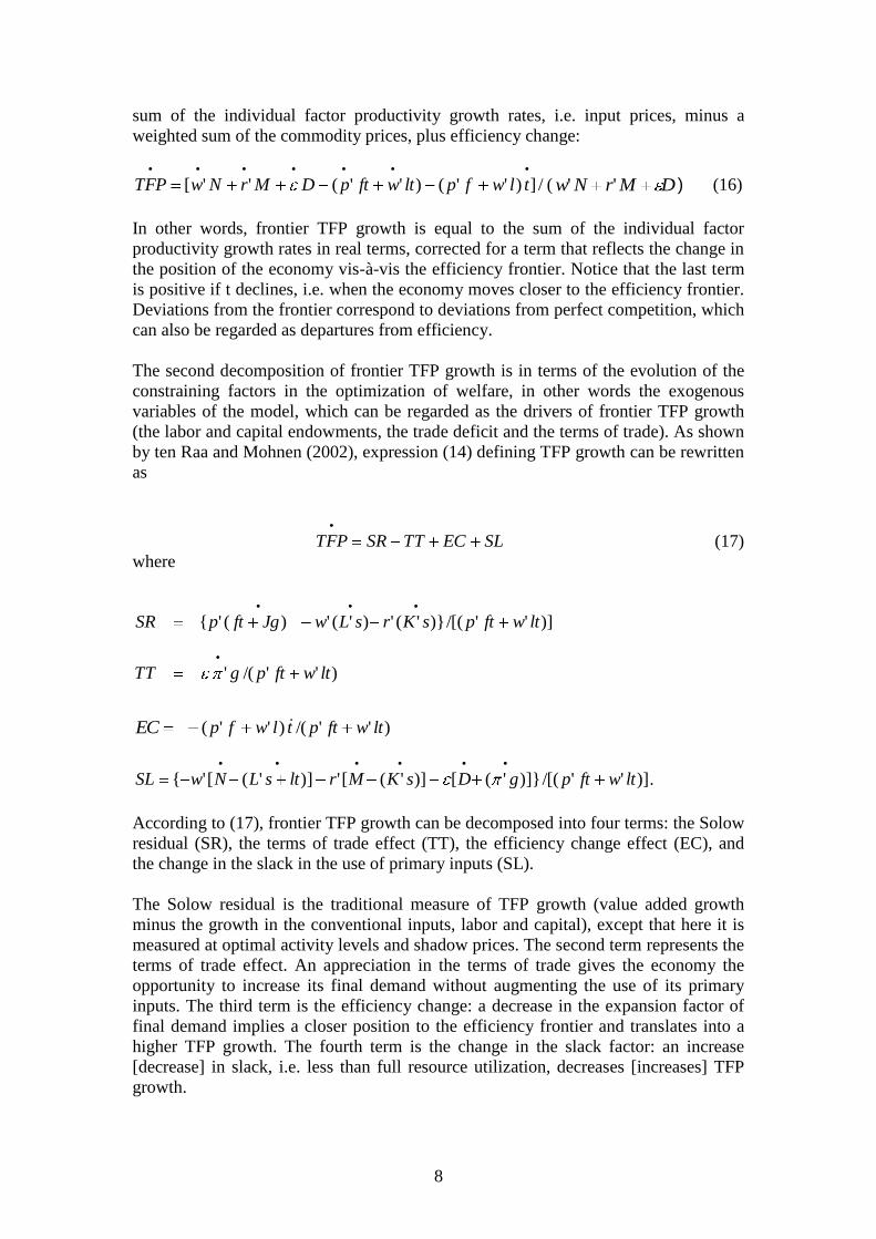
Table 2 reports the weighted average observed and optimal rates of return on
buildings, equipment and the total capital stock. The optimal rate of return on
buildings is the shadow price of constraint (8). The optimal rate of return on
equipment is the weighted of the shadow prices of constraints (7). The optimal rate of
return on the total capital stock is the weighted average of the shadow prices of
buildings and equipment. To calculate the observed rates of return on buildings and
equipment we followed the method used by the World Bank (World Bank, 1995).
Assuming that interest payments are fully deductible, as they are in Tunisia, the user
cost of physical capital is defined as: c = q (r (1 - t) + d), where q is the physical
capital deflator (specific to each sector and each component of the capital stock), r is
the real lending rate4, t is the corporate tax rate
5, and d is the depreciation rate (again
specific to each sector and component of the capital stock)6. Fiscal and financial
incentives have not been taken into account. The observed user cost for total capital is
the weighted average of the observed user costs for buildings and equipment. As
equipment depreciates faster than buildings the observed user cost of equipment is
higher than the observed user cost of buildings. The same does not necessarily hold
for the shadow prices of buildings and equipment.
The weighted average rate of return on physical capital dropped from 26.9 per cent in
1983 to 11 per cent in 1995 and rose afterwards to 30.8 per cent in 2001 (table 2). The
social return on capital decreased after the structural adjustment program got
4 The lending rate used is the money market rate plus 3 percentage points. Different preferential
sectoral interest rates were not taken into consideration. 5 To simplify the calculation, a 50% flat tax rate is applied for 1983-88, and after the tax reform in 1989
the normal corporate tax of 35% is applied for 1989-2001. Different tax rates for wholly exporting and
agricultural enterprises and various tax holidays have not been considered. 6 The average depreciation rate is of 2.9% for building and 6.7% for equipment.

7
introduced showing that the Tunisian economy invested during this period and rates
of return on capital got closer to the normal rate. From 1996 onwards, capital became
more scarce again, even more than in 1983.
Table 3 compares for selected years the shadow and the observed commodity prices.
We can distinguish two sub-periods. From 1983 to 1989 the shadow commodity
prices that sustain the optimal allocation of resources in the competitive benchmark
were higher than the observed commodity prices. Remember that in competitive
equilibrium prices may not exceed average cost (equation 10). Therefore we can
conclude that to survive in a competitive environment sectors would have had to price
their output at higher than observed prices. Commodity prices were kept artificially
low by regulation. Before the structural adjustment program, the price-fixing policy
depressed competition in many sectors and discouraged innovation (Ghali (1995),
Morrisson and Talbi (1996)). After 1989 the shadow commodity prices were below
the observed prices, except for electricity and water, which implies that the non-utility
sectors earned rents.
IV. The evolution of Tunisia’s economic potential, 1983-2001
We now turn to the definition and decomposition of frontier TFP growth. We define
frontier TFP growth as the growth of final demand of business and non-business
goods and services (where business goods and services refer to those for which there
is an intermediate demand) minus the growth in the primary inputs (the endowments
of the five types of labor, the capital stocks in each sector and the current trade
deficit):
DMrNw
DMrNw
lwfp
lwfpTFP
''
)''(
''
)''(
...... (14)
where dots denote growth rates. This new definition of frontier TFP growth is a
natural extension of the TFP concept at the sector level. Instead of computing the
growth of production not due to the growth of the factors of production (the
conventional definition of TFP growth), in an open economy and a macro-wide
context TFP is defined as the growth in final domestic demand that cannot be
explained by the growth in primary factor endowments. We call it frontier TFP
growth because we measure it at the prices (or marginal productivities) and general
activity level that solve the optimal program of resource allocation.
There are two ways to decompose frontier TFP growth. The first decomposition is in
terms of the individual factor productivities. We start from the equality between the
optimal values of the primal and the dual of the linear program, as stated by the first
theorem of linear programming:
DMrNwDFDt '' . (15)
By doing so, we position ourselves at the frontier of the economy. If we totally
differentiate (15) and make use of the normalization rule (11) we obtain, as derived by
ten Raa and Mohnen (2002), that frontier TFP growth can be written as the weighted
8
sum of the individual factor productivity growth rates, i.e. input prices, minus a
weighted sum of the commodity prices, plus efficiency change:
/])''()''(''[
.......tlwfpltwftpDMrNwTFP ( DMrNw '' ) (16)
In other words, frontier TFP growth is equal to the sum of the individual factor
productivity growth rates in real terms, corrected for a term that reflects the change in
the position of the economy vis-à-vis the efficiency frontier. Notice that the last term
is positive if t declines, i.e. when the economy moves closer to the efficiency frontier.
Deviations from the frontier correspond to deviations from perfect competition, which
can also be regarded as departures from efficiency.
The second decomposition of frontier TFP growth is in terms of the evolution of the
constraining factors in the optimization of welfare, in other words the exogenous
variables of the model, which can be regarded as the drivers of frontier TFP growth
(the labor and capital endowments, the trade deficit and the terms of trade). As shown
by ten Raa and Mohnen (2002), expression (14) defining TFP growth can be rewritten
as
SLECTTSRTFP
. (17)
where
)]''/[()}'(')'(')('{
...ltwftpsKrsLwJgftpSR
)''/('
.ltwftpgTT
EC )''/()''( ltwftptlwfp
)]''/[(]})'([)]'(['])'(['{
......ltwftpgDsKMrltsLNwSL .
According to (17), frontier TFP growth can be decomposed into four terms: the Solow
residual (SR), the terms of trade effect (TT), the efficiency change effect (EC), and
the change in the slack in the use of primary inputs (SL).
The Solow residual is the traditional measure of TFP growth (value added growth
minus the growth in the conventional inputs, labor and capital), except that here it is
measured at optimal activity levels and shadow prices. The second term represents the
terms of trade effect. An appreciation in the terms of trade gives the economy the
opportunity to increase its final demand without augmenting the use of its primary
inputs. The third term is the efficiency change: a decrease in the expansion factor of
final demand implies a closer position to the efficiency frontier and translates into a
higher TFP growth. The fourth term is the change in the slack factor: an increase
[decrease] in slack, i.e. less than full resource utilization, decreases [increases] TFP
growth.

9
In table 4 and in subsequent tables we present the evolution of Tunisian frontier TFP
growth and its components over the whole sample period (1983-2001) and different
sub-periods, corresponding respectively to the 6th
(1982-1986), 7th
(1987-1991), 8th
(1992-1996) and 9th
(1997-2001) five-year Economic Development Plans.
As table 4 reveals, over the whole sample period (1983-2001) frontier TFP growth
increased by a mere 0.2% per year. This poor global performance is especially due to
the negative growth rates over the 1983-1986 period, when frontier TFP actually
declined, in other words the economy’s potential seriously deteriorated. After 1986,
frontier TFP growth became positive again at about 1% per year. Regarding the
decomposition of TFP growth into the input sources and beneficiaries of TFP growth,
we notice that among the workers only manual workers and machine operators, i.e.
the unskilled workers, play a major role. The shadow wage of machine operators
increased in the first three periods and turned negative in the last period. For manual
workers, the least qualified workers, it flipped from negative (or zero) to positive in
each sub-period. The other categories of workers contributed only slightly to frontier
TFP growth because of their relative small share in total employment.
On the whole, capital, especially equipment, had a negative contribution to TFP
growth. Tunisia overinvested in equipment (see table 5). This was strikingly so during
the 1983-1986 sub-period. The declines in equipment after 1991 were beneficial to
aggregate TFP growth. The capital stock in buildings increased by 4.2% on average
over the whole period. The increase was justified in terms of increasing potential TFP
in 1983-1986, but no more afterwards. It must be recalled that in the period stretching
from 1972 to 1985 real interest rates were negative in selected key sectors (Morrisson
and Talbi (1995), World Bank (1996)). Investment policy changed in 1987.
Investment which previously had to be approved was now given financial and fiscal
incentives in some priority sectors. In 1993 a more unified code of investment was
promulgated which was based on export promotion, regional development, and
technological development.
The last primary input in our open model is the allowable trade deficit. Over the
whole period it played a slightly negative but modest role in frontier TFP growth. The
marginal value in terms of domestic final demand of one additional dinar of allowable
trade deficit decreased by one tenth of a percentage point throughout the period.
Commodity prices kept decreasing over time, thereby increasing the individual factor
productivities in real terms. The optimal expansion of domestic final demand
increased after 1992, which means that the economy moved further away from its
efficiency frontier.
We now turn to the decomposition of frontier TFP growth in terms of the growth in
the quantities of the exogenous variables. The Solow residual grew by 1% per year
over the whole period. In 1983-1986 it actually regressed, but then it rose in the next
three sub-periods to reach an annual growth rate of 2.2% in 1997-2001. The
improvement in the Solow residual coincides with the structural adjustment program
started in 1987. This policy aimed at increasing competition, liberalizing prices, the
financial sector and foreign trade, reforming public enterprises, and privatizing certain
sectors like the textile and the hotel industries. These reforms have been accelerated
and amplified after the implementation of the industrial restructuring program in
1996.

10
What is striking is the strong negative effect the terms of trade exerted on frontier TFP
growth in the two sub-periods prior to 1992 and after 1997. The evolutions of world
prices and of the exchange rate of the Tunisian dinar were not favorable to Tunisia.
On average the price of imported goods rose more than the price of exported goods. In
the end the Tunisian economy experienced over the whole period a significant drop in
its purchasing power on world markets. Only in 1992-1996 was the evolution of the
world prices compared to the domestic prices sustaining the equilibrium favorable to
Tunisia. The terms of trade effect neutralized so to say the Solow residual effect.
While Tunisia managed to move its efficiency frontier outwards after 1986 (Solow
residual), it also moved away from its efficiency frontier after 1992, as already
noticed in the first frontier TFP decomposition. Changes in the slacks of resource
utilization played only a minor role.
V. Sector decomposition of Tunisia’s Solow residual, 1983-2001
The decompositions of TFP growth in (16) and (17), and in particular the Solow
residual component, are decompositions at the macroeconomic level in a general
equilibrium setting. However, we can also define sector Solow residuals that are
consistent with the macroeconomic Solow residual by the Domar aggregation rule
(see Hulten (1978)). Let j stand for sectors, i for commodities, and k for groups of
sectors. The Solow residual for sector-group k can then be written as:
kj ijjii
kjjjjjj
kj ijjii
kjjjjj
kj ijjii
kj ijijjiji
kj ijjii
kj ijjijjii
kSRsvp
sKsKr
svp
sLsLw
svp
susup
svp
svsvp )()(')()( '
Notice that when k = j , we get the Solow residual for sector j.
According to the Domar aggregation rule:
kk
kj ijjii
SRltwftp
svp
SR)''(
(18)
We can thus define sector Solow residuals that by the Domar aggregation rule are
consistent with our Solow residual component of frontier TFP growth. The Domar
weights represent the ratio of optimal sector production and aggregate domestic final
demand. Each sector gets a weight proportional to its direct and indirect (via inter-
industry transactions) contribution to domestic final demand. The Domar weights add
thus up to more than 1.
Table 6 gives the weights used in the Domar aggregation of the sector Solow residuals
to get to the aggregate Solow residual, which forms part of our second frontier TFP
decomposition (equation (17)). Over the whole period the greatest weight is attached
11
to services followed by textile, food processing, agriculture, and mechanical and
electrical goods. The latter experienced a tremendous increase in its importance from
an average of 2% in 1983-1986 to an average of 28% in 1997-2001. This change in
industrial composition followed the government's decision to stop the assembly of
private cars and negotiate with European car manufacturers the "rules of local
content" for the import of the European cars. This decision led the initial growth of
this sector and an increased vertical integration with the E.U car industry (World
Bank, 2008). In contrast, the hydrocarbons sector’s importance in its contribution to
domestic final demand fell from 26% to 4% over the first and the last sub-periods.
In table 7 we compare the sector Solow residuals calculated at the activity levels and
shadow prices that sustain the optimal general equilibrium with those calculated at
observed activity levels and observed prices. It should first be noticed that the
observed Solow residuals overestimate in general the Solow residuals consistent with
the optimal program. The difference between the two measures is perhaps most
evident in the case of mining. In the optimal allocation of resources mining should not
be activated. It would be more economical to specialize in sectors where Tunisia has a
comparative advantage and use the import proceeds to import the mining goods.
Consequently there is no Solow residual for mining at the optimal activity level. In
practice, though, there is activity in mining and hence also a Solow residual, which is
actually sizeable. Over the period 1983-2001 the Solow residual evaluated at the
optimal allocation of resources was highest in electricity, water, and hydrocarbons.
Those are the strong sectors of the Tunisian economy. But it is also worth noticing
that the mechanical, electrical and textile goods sectors that faced increased
international competition maintained a high Solow residual, implying that they were
able to adjust to increased competitiveness. Substantial improvements in the Solow
residual took place in the services sectors that turned from negative before 1991 to
positive afterwards in contrast to agriculture whose Solow residual continuously
declined. The Tunisian economy is thus well under way in moving from a primary to
a tertiary economy.
VI. Conclusion
In this study we have examined the evolution of frontier TFP in Tunisia over the
period 1983-2001 using the framework of ten Raa and Mohnen (2002). Frontier TFP
growth captures the shift in the production frontier of the economy as well as
variations in efficiency movements with respect to the frontier. The location of the
frontier is obtained by the resolution of a linear program (or activity analysis) at the
level of the whole economy, taking into account factor resource constraints, inter-
industry linkages, preferences and world prices. We have proceeded to two
decompositions of TFP growth. One decomposes it with respect to the individual
marginal productivities: capital subdivided into buildings and equipment, labor
subdivided into five levels of qualification, and the allowable trade deficit. The
second one is with respect to the exogenous variables of the model, yielding four
terms: the usual Solow residual (but evaluated at frontier quantities and supporting
prices), the terms of trade effect, the economy’s efficiency and the extent of
incomplete resource utilization.
The main results of our analysis can be summarized in the following points:

12
Between 1983 and 2001 frontier TFP growth hardly increased in Tunisia. This poor
global performance is especially due to the negative growth rates over the 1983-1986
period, where the economy’s potential actually deteriorated. After the introduction of
the structural adjustment program, frontier TFP growth increased by about 1% per
year.
With the exception of the last sub-period corresponding to the 9th Five-Year
Development Plan, it was labor productivity and not capital productivity that was the
main contributor to frontier TFP growth, and in particular unskilled labor. The
allowable trade deficit played a slightly negative but modest role in frontier TFP
growth over the whole period. Commodity prices kept decreasing all the time, thereby
increasing frontier TFP growth.
The Solow residual computed at frontier levels grew by 1% per year over the whole
period and kept increasing after the structural adjustment program, which started in
1987. It even accelerated after the implementation of the industrial restructuring
program in 1996. What is striking is the strong negative effect the terms of trade
exerted on frontier TFP growth in all sub-periods, except between 1992 and 1996. The
evolution of world prices and the value of the Tunisian dinar were not favorable to
Tunisian frontier TFP growth. Tunisia managed more efficiently its primary resources
until 1992, and then it moved away from its efficiency frontier while the frontier kept
moving outwards.
These results indicating changing trends and deep restructurings in the Tunisian
economy should nevertheless be taken with some reservations. Nugent (1970) already
pointed out that activity analysis models like this one may depend heavily on model
and data imperfections. Data on capacity utilizations and labor force by type of
qualification are partly constructed and hence particularly subject to measurement
errors. Quantities are hard to measure in the service sectors and future studies will
certainly improve our measure of productivity in services. The same could be said
about quality changes with possible mismeasurement of output, especially in high-
tech commodities. It would be more rewarding to have a disaggregation of labor by
skills rather than by occupations. Finally, adjustment lags and expectations are
completely absent from this static model. Introducing dynamics into the model would
call for an intertemporal optimization model. It may well be that what is regarded as
bad performance in the short run could turn out to be beneficial in a long-run
perspective.

13
Bibliography
Balk, B. (1998), Industrial Price, Quantity, and Productivity Indices: The Micro-
Economic Theory and an Application. Kluwer Academic Publishers, Boston.
Barro, R. J. (1999), "Notes on Growth accounting", Journal of Economic Growth, 4,
119-137.
Bsaies, A., M. Goaied et R. Baccouche (1995), "Etude de la productivité globale des
facteurs: Analyse globale", Notes et Documents de Travail, No 04-95, Institut
d'Economie Quantitative, Septembre.
Bosworth, B., S. Collins and Y. C. Chen (1995), "Accounting for Differences in
Economic Growth", Brookings Discussion Papers in International Economics,
No 115.
Caves, D.W., L.R. Christensen and W.E. Diewert (1982), "The Economic Theory of
Index Numbers and the Measurement of Input, Output, and Productivity",
Econometrica, 50, 1393-1414.
Diewert, W. E. (1976), "Exact and Superlative Index Numbers", Journal of
Econometrics, 4, 115-145.
Diewert, W. E. (1981), "The Theory of Total Factor Productivity Measurement in
Regulated Industries", in Cowing, T. and R. Stevenson (eds.), Productivity
Measurement in Regulated Industries, Academic Press, New York.
Diewert, W. E. (1992), "The Measurement of Productivity", Bulletin of Economic
Research, 44(3), 163-198.
Diewert, W. E. and C.J. Morrison (1986), "Adjusting Output and Productivity Indexes
for Change in the Terms of Trade", Economic Journal, 96, 659-679.
Domar, E. (1961), "On the Measurement of Technical Change", Economic Journal,
70, 710-729.
Färe, R., Grosskopf S., Norris M. and Zhang Z. (1994), "Productivity Growth,
Technical Progress, and Efficiency Change in Industrialized Countries", American
Economic Review, 84, 1, March, 66-83.
Farrell, M. J. (1957), "The Measurement of Productivity Efficiency", Journal of Royal
Statistical Society A, 120, 253-281.
Fuentes, H.J., E. Grifell-Tatjé, and S. Perelman (2001), "A Parametric Distance
Function Approach for Malmquist Productivity Index Estimation", Journal of
Productivity Analysis, 15, 79-94.
Ghali, S. (1995), "Régimes des prix et organisation de la concurrence", in Schéma
Global de Développement de l'Economie Tunisienne à l'Horizon 2010, Etude
stratégique No 3, Vol III, Institut d'Economie Quantitative, Novembre.

14
Ghali, S. and P. Mohnen (2003), "Restructuring and Economic Performance: The
Experience of the Tunisian Economy", in Trade Policy and Economic Integration in
the Middle East and North Africa: Economic Boundaries in Flux, (Hassan Hakimian
and Jeffrey B Nugent, eds.), London: Routledge-Curzon.
Grosskopf, S. (2001), "Some Remarks on Productivity and its Decompositions",
mimeo.
Hall, R.E. (1990), "Invariance Properties of Solow's Residual", in Diamond, P. (ed.),
Growth / Productivity / Unemployment, M.I.T Press, Cambridge, M.A.
Hulten, C. R. (1978), "Growth Accounting with Intermediate Inputs", Review of
Economic Studies, 45, 511-518.
Institut d’Économie Quantitative (1996), Étude stratégique No. 8, compétitivité,
restructuration, diversification et ouverture sur l’extérieur des industries
manufacturières et des services, 8622/96.
Institut National de la Statistique, Les comptes de la nation.
International Monetary Fund (1999), Tunisia: Staff Report for the Article IV
Consultation, IMF Staff Country Report No. 99/104, September, Washington D.C.
Jorgenson, D. W. and Z. Griliches (1967), "The Explanation of Productivity Change",
Review of Economic Studies, 34(3), 308-350.
Kohli, U. (1991), Technology, Duality, and Foreign Trade: The GNP Function
Approach to Modelling Imports and Exports, Ann Arbor: University of Michigan
Press.
Ministère du Développement Economique et de la Coopération Internationale (1992),
VIII ème Plan de Développement, 1992-1996, Contenu Global, Vol I, République
Tunisienne.
Ministère du Développement Economique et de la Coopération Internationale (1996),
IX ème Plan de Développement, 1996-2001, Contenu Global, Vol I, République
Tunisienne.
Morrisson, C. and B. Talbi (1996), La croissance de l’économie tunisienne en longue
période. Centre de développement de l’OCDE.
Nugent, J. (1970), "Linear Programming Models for National Planning:
Demonstration of a Testing Procedure", Econometrica, 38(6), 831-855.
Redjeb, M.S. et B. Talbi (1995), "Performance de l'Economie Tunisienne durant la
Période 1961-1993", in Schéma Global de Développement de l'Economie Tunisienne
à l' Horizon 2010, Etude stratégique No 3, Vol II, Institut d'Economie Quantitative,
Novembre.

15
Redjeb, M. S. et L. Bouzaiane (1999), "Contribution du secteur privé à la croissance
économique en Tunisie", in L'entreprise au seuil du troisième millénaire: Défis et
Enjeux, Institut Arabe des Chefs d'Entreprises, Novembre.
Solow, R. (1957), "Technical Change and the Aggregate Production Function",
Review of Economics and Statistics, 39, 312-320.
ten Raa, T. and P. Mohnen (2002), " Neoclassical Growth Accounting and Frontier
Analysis: A Synthesis ", Journal of Productivity Analysis, 18, 111-128.
World Bank (1995), Republic of Tunisia, Poverty Alleviation: Preserving Progress
while Preparing for the Future, Report No. 13993-TUN, Vol II, August. Washington
D.C.
World Bank (1996), Tunisia's Global Integration and Sustainable Development,
Strategic Choices for the 21. Washington D.C.
World Bank (2000a), Tunisia-Private Sector Assessment Update, Meeting the
Challenge of Globalization, report No.20173-TUN, December. Washington D.C.
World Bank (2000b), Republic of Tunisia. Social and Structural Review 2000.
Washington D.C.
World Bank (2008), Tunisia's Global Integration: Second Generation of Reform to
Boost Growth and Employment, report No.40129-TUN, May. Washington D.C.

16
Table 1
Observed and shadow prices of labor for different levels of qualification (1983-2001).
(1,000 DT per year, 1990 prices)
L 1 L 2 L 3 L 4 L 5
observed shadow observed shadow observed shadow observed shadow observed shadow
1983 1.143 0.246 1.934 0.246 2.968 0.246 4.158 0.246 5.605 0.246
1984 1.109 0.846 1.913 0.846 3.025 0.846 4.039 0.846 5.450 0.846
1985 1.015 1.832 1.983 1.832 2.639 1.832 3.648 1.832 5.059 1.832
1986 1.007 0.340 1.689 0.749 2.621 0.749 3.858 0.749 5.047 0.749
1987 0.874 0.781 1.740 0.781 2.422 0.781 3.211 0.781 4.365 0.781
1988 0.954 0.000 1.591 0.472 2.477 0.472 3.713 0.472 4.810 0.472
1989 0.906 0.016 1.742 0.016 2.447 0.016 3.243 0.016 4.556 0.016
1990 1.000 1.451 1.617 1.451 2.466 1.451 3.760 1.451 5.036 1.451
1991 0.929 1.581 1.788 1.581 2.385 1.581 3.358 1.581 4.671 1.581
1992 1.097 1.242 1.752 1.242 2.786 1.242 3.844 1.242 5.516 1.242
1993 1.016 1.282 1.919 1.282 2.646 1.282 3.474 1.282 5.172 1.282
1994 1.125 1.743 1.788 1.992 2.765 1.992 3.829 1.992 5.657 1.992
1995 1.065 0.599 1.838 3.221 2.236 3.221 3.591 3.221 5.403 3.221
1996 1.200 0.177 1.756 2.050 3.007 2.050 4.138 2.050 6.080 2.050
1997 1.214 0.000 1.879 2.040 3.010 2.040 4.219 2.040 6.102 2.040
1998 1.219 0.000 1.880 0.000 3.004 0.000 4.266 0.000 6.164 0.000
1999 1.272 0.000 1.915 0.000 3.183 0.000 4.373 0.000 6.403 0.000
2000 1.315 0.000 1.943 0.000 3.349 0.000 4.506 0.000 6.603 0.000
2001 1.364 1.659 2.006 1.659 3.442 1.659 4.647 1.659 6.866 1.659
L1: manual workers/trainees, L2: machine operators, L3: foremen, L4: technicians, L5: engineers/administrators
DT: Tunisian Dinar
17
Table 2
Observed and shadow weighted average of sector level rates of return of capital stock (K)
decomposed into buildings (KB) and equipment (KE) (1983-2001).
(Weighted average of sector level rates of return, expressed in base-year (1990) prices).
Total capital Equipment Buildings
observed optimal observed optimal observed optimal
1983 0.026 0.269 0.027 0.308 0.024 0.219
1984 0.032 0.209 0.033 0.229 0.031 0.183
1985 0.045 0.166 0.047 0.178 0.043 0.151
1986 0.054 0.193 0.057 0.145 0.049 0.253
1987 0.057 0.189 0.068 0.142 0.044 0.245
1988 0.062 0.209 0.076 0.199 0.047 0.221
1989 0.076 0.214 0.093 0.156 0.058 0.279
1990 0.102 0.148 0.122 0.111 0.081 0.188
1991 0.100 0.143 0.123 0.096 0.076 0.192
1992 0.127 0.181 0.152 0.128 0.100 0.235
1993 0.140 0.188 0.171 0.165 0.110 0.211
1994 0.125 0.160 0.158 0.169 0.093 0.152
1995 0.114 0.110 0.152 0.093 0.082 0.125
1996 0.147 0.194 0.201 0.204 0.102 0.186
1997 0.137 0.188 0.198 0.188 0.090 0.187
1998 0.147 0.294 0.214 0.356 0.098 0.249
1999 0.145 0.299 0.213 0.389 0.098 0.238
2000 0.142 0.301 0.208 0.482 0.098 0.183
2001 0.156 0.308 0.223 0.216 0.114 0.199

18
Table 3
Observed (obs.) and shadow (shad.) commodity prices (selected years).
(base year: 1990)
1984 1987 1990 1993 1996 1999 2001
obs. shad. obs. shad. obs. shad. obs. shad. obs. shad. obs. shad. obs. shad.
Agric & Fishing 0.658 0.855 0.794 0.837 1.000 0.951 1.120 0.901 1.227 0.786 1.315 0.774 1.426 1.030
Food process 0.650 0.771 0.838 0.885 1.000 0.951 1.167 0.721 1.397 1.104 1.515 0.880 1.596 0.702
Const material 0.762 1.175 0.840 1.081 1.000 0.951 1.147 0.988 1.241 0.909 1.311 1.086 1.385 1.331
Mechan & Elect 0.616 0.969 0.775 1.050 1.000 0.951 1.116 1.067 1.263 0.867 1.409 1.431 1.490 1.255
Chem & Rubb 0.747 1.515 0.814 1.092 1.000 0.951 1.083 0.864 1.329 0.926 1.385 0.989 1.368 0.779
Text & Leather 0.592 0.970 0.767 1.019 1.000 0.951 1.217 1.085 1.434 1.028 1.553 1.085 1.619 0.912
Other Manuf 0.654 0.919 0.790 0.983 1.000 0.951 1.136 1.068 1.209 0.907 1.306 1.106 1.371 0.855
Mining 0.902 1.405 0.743 0.913 1.000 0.951 0.906 0.964 1.188 0.709 1.526 0.881 1.514 0.738
Hydrocarbons 0.868 1.955 0.867 1.016 1.000 0.951 0.992 0.775 1.042 0.745 1.156 0.722 1.447 1.064
Electricity 0.886 2.377 0.951 1.960 1.000 1.506 1.108 1.447 1.219 1.268 1.345 1.461 1.443 1.480
Water 0.714 2.700 0.858 3.198 1.000 2.700 1.177 2.681 1.366 2.408 1.437 2.524 1.508 2.274
Construction 0.707 0.841 0.828 0.846 1.000 0.879 1.210 0.877 1.281 0.862 1.424 0.783 1.494 0.940
Transp &Comm 0.681 1.188 0.855 1.127 1.000 0.951 1.222 1.086 1.294 0.941 1.327 1.011 1.416 0.909
Hot & Tourism 0.648 1.234 0.804 1.103 1.000 0.951 1.268 1.165 1.533 1.033 1.719 1.056 1.788 0.886
Other Services 0.578 1.222 0.826 1.089 1.000 0.951 1.183 1.056 1.349 0.982 1.468 1.067 1.575 0.918

19
Table 4
Decomposition of Frontier Total Factor Productivity Growth (1983-2001 and various sub-periods)
1983-2001 1983-1986 1987-1991 1992-1996 1997-2001
TOTAL 0.2 -4.6 1.0 1.1 1.0
Manual workers and trainees
Machine operators
Foremen
Technicians
Engineers/administrators
Equipment
Buildings
Trade deficit
Changes in commodity prices
Efficiency
---------------------------------------
Solow Residual
Terms of trade
Efficiency
Resource utilization
0.3
0.8
0.1
0.1
0.1
-1.4
-0.1
-0.1
0.2
0.2
-----------------
1.0
-1.0
0.2
0.0
0.0
1.2
0.2
0.3
0.1
-10.0
2.3
-0.1
0.6
0.8
-------------------
-2.5
-2.7
0.8
-0.2
1.3
2.8
0.4
0.4
0.2
-3.0
-2.4
-0.1
0.2
1.2
-------------------
0.8
-0.8
1.2
-0.2
-1.4
2.5
0.4
0.3
0.2
2.6
-2.1
-0.1
0.1
-1.4
-------------------
1.5
0.7
-1.4
0.3
1.7
-1.6
-0.2
-0.2
-0.1
1.0
0.5
-0.1
0.1
-0.1
------------------
2.2
-1.0
-0.1
-0.1
20
Table 5
Annual growth rates of labor (by type), capital (by type) and trade deficit
(in percentages)
1983-2001 1983-1986 1987-1991 1992-1996 1997-2001
Manual workers and trainees 1.1 0.2 1.7 0.6 1.2
Machine operators 2.9 3.5 3.0 2.8 2.8
Foremen 3.0 3.2 3.8 3.1 3.2
Technicians 2.9 1.5 2.8 3.3 2.6
Engineers/administrators 3.5 7.0 2.6 3.1 2.9
Total labor 2.5 2.6 2.7 2.3 2.5
Equipment 0.6 4.9 0.3 -1.1 -0.5
Buildings 4.2 5.9 3.4 4.7 4.5
Total capital 2.6 5.3 1.7 2.0 2.5
Trade deficit -0.2 -12.8 13.1 -64.6 34.1

21
Table 6
Solow residual (SR) at optimal activity levels and shadow prices (1983-2001), (annual growth rates in percentages)
and mean weights in Domar aggregation
1983-2001 1983-1986 1987-1991 1992-1996 1997-2001
SR weights SR weights SR weights SR weights SR weights
Agriculture and fishing -0.1 0.21 -0.2 0.24 -0.3 0.26 -2.2 0.21 -2.1 0.12
Food processing 0.7 0.24 -0.4 0.11 -0.6 0.34 -0.6 0.14 4.2 0.26
Construction materials & glass 1.5 0.02 10.0 0.00 0.0 0.00 0.7 0.00 -1.5 0.11
Mechanical and electrical goods 1.0 0.20 0.6 0.02 0.7 0.20 0.7 0.19 2.7 0.28
Chemical and rubber products 0.8 0.00 0.0 0.00 0.0 0.00 7.8 0.00 1.2 0.00
Textile and leather products 1.1 0.24 1.2 0.10 1.2 0.24 1.3 0.27 1.1 0.29
Other manufacturing 0.6 0.09 0.8 0.01 0.2 0.10 0.9 0.10 0.2 0.11
Mining 0.0 0.00 0.0 0.00 0.0 0.00 0.0 0.00 0.0 0.00
Hydrocarbons 1.7 0.11 1.1 0.26 1.5 0.13 -3.4 0.04 8.5 0.04
Electricity 1.5 0.04 0.5 0.03 2.8 0.04 1.6 0.03 0.7 0.05
Water 1.2 0.02 0.2 0.02 -0.5 0.03 1.9 0.02 1.6 0.02
Construction and public works 0.7 0.15 1.5 0.16 0.5 0.12 1.6 0.17 0.9 0.16
Transport and telecom. 0.9 0.11 -0.8 0.06 -0.1 0.08 1.2 0.15 1.3 0.17
Hotel and tourism 0.4 0.13 -1.2 0.12 -2.8 0.13 1.5 0.14 0.7 0.13
Other services -0.1 0.43 -5.2 0.44 -0.4 0.42 2.3 0.42 1.0 0.45
Aggregate 1.0 1.97 -2.5 1.58 0.8 2.09 1.5 1.87 2.2 2.19

22
Table 7
Sector Solow residuals at observed and optimal prices and activity levels (1983-2001) (annual growth rates in percentages)
1983-2001 1983-1986 1987-1991 1992-1996 1997-2001
observed optimal observed Optimal Observed optimal observed optimal observed optimal
Agriculture and fishing 1.6 -0.1 1.7 -0.2 1.4 -0.3 -0.9 -2.2 0.0 -2.1
Food processing 0.8 0.7 1.9 -0.4 -0.4 -0.6 0.3 -0.6 0.8 4.2
Construction materials & glass 1.1 1.5 -0.4 10.0 0.0 0.0 3.3 0.7 1.6 -1.5
Mechanical and electrical goods 1.1 1.0 1.4 0.6 0.9 0.7 0.7 0.7 2.1 2.7
Chemical and rubber products 0.5 0.8 1.0 0.0 1.6 0.0 0.3 7.8 0.0 1.2
Textile and leather products 1.4 1.1 1.1 1.2 1.9 1.2 1.5 1.3 1.3 1.1
Other manufacturing 0.8 0.6 2.0 0.8 0.2 0.2 0.8 0.9 0.3 0.2
Mining 1.8 0.0 0.5 0.0 0.8 0.0 0.4 0.0 3.9 0.0
Hydrocarbons 0.7 1.7 2.6 1.1 1.6 1.5 0.0 -3.4 -1.2 8.5
Electricity 0.2 1.5 2.5 0.5 0.0 2.8 0.9 1.6 -2.3 0.7
Water 1.4 1.2 0.4 0.2 -3.3 -0.5 5.3 1.9 2.1 1.6
Construction and public works 0.9 0.7 -0.3 1.5 0.7 0.5 1.9 1.6 2.5 0.9
Transport and telecom. 2.0 0.9 0.2 -0.8 0.1 -0.1 4.1 1.2 2.0 1.3
Hotel and tourism 1.4 0.4 1.0 -1.2 -2.0 -2.8 1.7 1.5 1.7 0.7
Other services 1.1 -0.1 -2.7 -5.2 1.4 -0.4 1.6 2.3 2.5 1.0
Aggregate 2.2 1.0 0.8 -2.5 1.4 0.8 2.2 1.5 2.6 2.2

23
Appendix I: Industry nomenclature and symbols
Industry Commodity code AGRICULTURE & FISHING
Agriculture & fishing 00
MANUFACTURING
Food processing 10
Construction materials & glass 20
Mechanical & Electrical goods 30
Chemical & Rubber products 40
Textile & Leather products 50
Other Manufacturing 60
UTILITIES
Mining 65
Hydrocarbons 66
Electricity 67
Water 68
Construction & Public works 69
SERVICES
Transport &Communications 76
Hotels & Tourism 79 + 99
- Hotels, coffees and restaurants 79
- Tourism and other stays 99
Other Services 72+ 82 + 85 + 94
- Commodity trade 72
- Financial services and insurance 82
- Other market services 85
- Non market services 94