Economic Policy Uncertainty & Asset Price Volatility∗

Maxim Ulrich

Columbia University

∗Contact details: mu2167@columbia.edu

Economic Policy Uncertainty & Asset Price Volatility

Abstract

We document that fear about misspecified economic and central bank policies explain 45%

of variations in bond option implied volatilities and interest rate volatilities. We endogenize

this empirical pattern with a parsimonious equilibrium asset pricing model. In equilibrium,

volatility is endogenously driven by fear of not knowing the data generating process that drives

future economic and future central bank policies. An increase in either of these two uncertainties

steepens the yield curve and increases the volatility in asset and option markets. A structural

estimation of the equilibrium model explains the upward sloping term structures of interest

rates, bond volatility, and option volatility, with only four in real-time observable economic and

central bank related risk and uncertainty factors. The study ends with highlighting an inverse

relationship between interest rates and volatility disparity from fundamentals during the policy

hiking period of 2004-2007 and during QE1.

1 Introduction

The Chairman of the Federal Reserve emphasizes in Bernanke and Kuttner (2005) the impor-

tance of understanding how monetary policy risks transmit to asset markets.1 Surprisingly, little

is known about how monetary policy and economic risks affect bond option markets and the

volatility of interest rates. Notice the strong co-movement of different standardized volatility

measures from Treasury bond and bond option markets in Figure 2. In fact, more than 90% of

variations in these volatilities are driven by one unobserved factor. Can observable measures of

economic and monetary policy risks account for at least a fraction of these variations? Is there

a simple and parsimonious asset pricing model that explains the transmission mechanism from

macroeconomic and monetary policy risks to the volatility of bonds and options? It is the goal

of this paper to answer these questions.

Guided by existing state of the art asset pricing theories, we divide economic and mone-

tary policy (inflation) risks into three subgroups: business cycle risk (’Activity’), volatility risk

(’Risk’), and model risk (’Uncertainty’).2 We document in Table 2 that (i) 50% of variations in

the above mentioned unobserved bond volatility factor are explainable by observable macroe-

conomic risk factors, (iii) variations in Activity and Risk seem not to drive the volatility in

the bond market, (iii) variations in Uncertainty soak up the entire 50% of explanatory power,

(iv) controlling for the yield curve does not drive out Uncertainty as an important contribu-

tor to bond volatility, and (v) economic and monetary policy Activity and Uncertainty are key

macroeconomic risk factors for variations in Treasury interest rates.

It is unfortunate for economic research in general and for the understanding of the monetary

policy transmission mechanism in particular, that existing asset pricing theories cannot explain

why Economic Uncertainty and Monetary Policy Uncertainty are such important volatility risk

factors in the bond and in the option market. We close this gap in the literature by proposing

a parsimonious equilibrium asset pricing model where asset price volatility is endogenously

driven by Economic Uncertainty and Monetary Policy Uncertainty.

The agent in our model is exposed to both, Knightian uncertainty about future Economic

Activity and Knightian uncertainty about future Monetary Policy Activity. Notice that com-

1 Bernanke and Kuttner (2005) write in their introduction: ”Understanding the links between monetary policy

and asset prices is thus crucially important for understanding the policy transmission mechanism.”2 Monetary policy risks and uncertainties relate to inflation because one of the key Federal Reserve mandates,

given by U.S. Congress, is to keep inflation under control. Even unconventional Quantitative Easing policies of

central banks around the globe were motivated as necessary tools to ensure stable inflation in the future.

1

pared to Risk, the investor is not afraid of not knowing the realized values of future Economic

Activity and future Monetary Policy Activity ex-ante, but instead he fears not to know their re-

spective data generating process (DGP). The time-varying magnitude of Economic Uncertainty

and Monetary Policy Uncertainty is exogenous and heteroscedastic and leads in equilibrium to a

heteroscedastic dynamic of marginal utility, interest rate volatility, and to stochastic option im-

plied volatilities. The model accounts very naturally for the high co-movement between interest

rate volatility and option implied volatility that is revealed in Figure 2.

Our goal is not to understand the reason for Uncertainty but its equilibrium effect onto the

volatility of interest rates and bond options. Our equilibrium model contributes several theo-

retical insights to the existing literature, from which we emphasize two. First, the source of

Uncertainty matters. An exogenous increase in Economic Uncertainty leads to a flight to safety

and a steepening of the yield curve because being long a Treasury bond hedges the amplified

amount of Economic Uncertainty. On the other hand, holding a Treasury bond does not hedge

run-ups in Monetary Policy Uncertainty. Second, an increase in Economic Uncertainty and/or

Monetary Policy Uncertainty leads to an endogenous increase in the volatility of interest rates

and in bond option implied volatilities. The relative persistence of both Uncertainty measures

and the relative strength of the agent’s fear determine whether Economic Uncertainty or Mon-

etary Policy Uncertainty dominates the endogenous dynamic of volatility in the bond market.

Whereas the persistence of both Uncertainty measures is pinned down by their respective time

series behavior, we have to estimate the equilibrium model to assess the agent’s degree of fear.

We estimate the structural model with Maximum Likelihood and a rich panel of interest rate,

macroeconomic, monetary policy, interest rate volatility, and bond option implied volatility

data. From the numerous empirical lessons, we want to stress six novel and policy relevant

insights.

First, the parsimonious equilibrium model is able to explain, the upward sloping term struc-

tures of interest rate volatility, option implied volatility, and interest rates. Second, fear (i.e.

Uncertainty) in the model is driven by two components, a high frequency component (i.e. Eco-

nomic Uncertainty) and a low frequency component (i.e. Monetary Policy Uncertainty). Third,

a potentially alarming finding for policy makers and central bankers is that the estimated half-

life of a shock to Monetary Policy Uncertainty is over 50 years. Fourth, the parsimonious

model captures that physical volatilities and option implied volatilities sharply increase before

recessions, which is mainly driven by an increase in Uncertainty about future Monetary Policy

Activity.

2

Fifth, according to our model, there was a significant underpricing of bond volatility during

2004 and 2007. This deviation from fundamentals was not caused by an artificially low market

price of volatility, but instead by an understatement of physical bond volatility. Sixth, the esti-

mated structural model reveals a striking negative correlation between Treasury yields starting

to revert back to fundamentals in 2004, and bond volatility starting to negatively deviate from

fundamentals. The Federal Reserve started to raise interest rates in 2004 to correct the path of

easy monetary policy that it launched right before the 2001 recession. The pricing errors of our

model suggest that the bond market might have interpreted that as a signal towards lower finan-

cial market risk ahead, despite the amount of fundamental uncertainty in the macroeconomy

(i.e. Monetary Policy Uncertainty) being unchanged. With the launch of untested QE1 policies

(Quantitative Easing), bond interest rates started to trend significantly lower than predicted by

fundamentals in our model, whereas bond volatilities started to move above fundamentals.

The theoretical results of our paper contribute to a very small but fast growing part of the lit-

erature that links volatility in financial markets to Knightian uncertainty about macroeconomic

fundamentals.3 Liu et al. (2005) analyze how Knightian uncertainty about rare events affects

equity options. The authors endogenize an uncertainty premium for exposure to rare events

and show in a calibration exercise its importance for the volatility of equity options. Drech-

sler (2012) endows an extended Bansal and Yaron (2004) economy with a representative agent

who is exposed to Knightian uncertainty about the frequency and magnitude of rare jumps in

endowment growth, cashflow growth, and their volatility. Holding a financial option provides a

natural hedge against these model misspecification concerns which, as a calibration shows, can

explain the high variance risk premium in S&P500 index options. Miao et al. (2012) extend

the smooth ambiguity model of Ju and Miao (2012) to account for the variance risk premium in

equity options. The authors show that ambiguity aversion enlarges the counter-cyclical nature

of the stock return variance and amplifies the variance risk premium in equity options.

These pioneering theoretical contributions study the effect of Knightian uncertainty on the

variance risk premium in equity options and calibrate their respective model to several uncon-

ditional financial and macroeconomic moments. Unlike these papers, our theory shuts off both

3 Theoretical contributions to link financial market volatility to Knightian uncertainty are rare, but the founda-

tions of the importance of Knightian uncertainty in financial economics is very rich. Early pioneers are Knight

(1921), Ellsberg (1961), Gilboa and Schmeidler (1989), Chen and Epstein (2002), Anderson, Hansen, and Sargent

(2003), Epstein and Schneider (2003), Uppal and Wang (2003), Klibanoff et al. (2005), Hansen et al. (2006),

Hansen and Sargent (2008). Applications to financial economics are Epstein and Miao (2003), Maenhout (2004,

2006), Sbuelz and Trojani (2008), Gagliardini et al. (2009), Ju and Miao (2012), among others.

3

the rare events and/or stochastic volatility channel in fundamentals, the variance risk premium,

and the dependence on unobserved risk factors. Instead, we explicitly analyze how Knight-

ian uncertainty about future economic and monetary policy actions affects the volatility in the

bond market. Another distinguishing feature of our modeling is the strong empirical focus of

our analysis. We focus explicitly on the time series properties of bond volatility and analyze

whether different types of observable macro and policy related risks and uncertainties account

for these. Our equilibrium model is more parsimonious than the existing theories and allows

for a straightforward maximum likelihood estimation with only observable macroeconomic risk

variables. The empirical part of our paper is the first to document that an equilibrium model with

Knightian uncertainty can indeed explain key features of interest rates, interest rate volatility,

and bond option implied volatilities.

Other equilibrium asset pricing theories with Knightian uncertainty that are tested with

empirical estimations are rare in the literature. Ulrich (2012) is the first study to document

that an equilibrium model with an observable amount of Knightian uncertainty about future

monetary policy actions is indeed able to explain a longstanding puzzle that the same model

without Knightian uncertainty could not resolve. Ulrich (2012) focuses on the positive term

premium in U.S. government bonds and can explain why the yield curve was rather flat in the

early 1980s, whereas observable forecasts of inflation were strongly downward sloping. He

shows that the observable amount of inflation uncertainty, measured as dispersion in profes-

sional macroeconomic forecasts, was strongly elevated during that time period. The ambiguity

averse representative investor did therefore price Treasury bonds with a steep inflation ambigu-

ity premium. While Wright (2011) provides international empirical evidence for the importance

of this channel, Ulrich (2012) cannot explain why Knightian uncertainty might affect the con-

ditional volatility of interest rates. Furthermore, his empirical implementation, following the

tradition in the literature, relies on unobserved factors, which complicates policy relevant in-

terpretations. Our study has a different focus because we focus on endogenizing volatility in

the bond and option market with only observable measures of economic and monetary policy

related Knightian uncertainty.

Another small but very important strand of the theoretical asset pricing literature tries to

link (primarily) equity volatility to the macroeconomy via Bayesian learning.4 In contrast to

4 Pioneering work in that field include Detemple and Murthy (1994), Zapatero (1998), David (1997), Veronesi

(1999), Veronesi (2000), David and Veronesi (2002), and Basak (2005). Buraschi and Jiltsov (2006) analyze how

learning about the endowment growth rate affects equity options and trading volume. Buraschi et al. (2009) study

how learning about cashflow growth affects the cross-section of credit spreads. David and Veronesi (2009) study

4

this exciting avenue of research, we show that a simple economy with Knightian uncertainty

and only four observable state variables is able to make a step towards linking bond and option

volatility to uncertainty about monetary policy. We leave a related analysis within a Bayesian

learning framework to future research.

The rest of the paper is organized as follows. Section 2 is devoted towards understanding the

empirical linkages between different types of macroeconomic risks and the volatility on bond

and option markets. Section 3 proposes an equilibrium model that endogenizes key features

of the lessons from Section 2. Section 4 presents the findings of the structural model estima-

tion. Section 5 concludes and all proofs, description of data, as well as the specification of the

likelihood function are summarized in the appendix.

2 Economic Risks and Bond Volatility

In this section we document that a significant fraction of volatility in Treasury bond and Trea-

sury bond option markets correlates with variations in observable measures of economic risks.

We differentiate between economic risks and risks associated with monetary policy. Monetary

policy risks are related to inflation because first, the Federal Reserve controls the aggregate

supply of money in the U.S. economy (and therefore inflation) and second, one of its mandate,

given by U.S. Congress, is to ensure low rates of inflation. We classify economic risks to be re-

lated to real economic growth in the economy. The analysis will decompose both economic and

monetary policy risks into three sub-categories each: Activity, Risk, and Uncertainty, which, as

we show below, builds naturally on state of the art economic theory and macroeconomic data.

2.1 Different Economic Risk Measures

Our primary focus of the empirical analysis is to understand whether economic and policy risks

could be responsible for variations in the volatility of bond markets. Guided by theory we differ-

entiate between business cycle risks, volatility risks (which assumes the data generating process

is known), and Knightian uncertainties. The seminal work of Knight (1921) emphasized the

importance of distinguishing between knowing the DGP but not knowing the outcome ex-ante

(volatility risk) from not knowing the DGP that the random variable is drawn from (Knightian

how learning affects the time-varying correlation between stocks and bonds, whereas David and Veronesi (2012)

analyze how learning about the Taylor rule affects the price of equity options.

5

uncertainty). The more recent seminal workhorse model of Bansal and Yaron (2004) empha-

sizes that innovations to business cycle variables can be important macroeconomic risk factors.

We call such risk factors Activity as by their nature, they capture economic and policy activity.

We use real-time data from the Survey of Professional Forecasters to account for all three

subcategories of economic and policy risks. We define the demeaned one quarter ahead median

GDP growth forecast to coincide with Economic Activity. Similarly, we define the demeaned

one quarter ahead median inflation forecast to coincide with Monetary Policy Activity. In order

to have a standard measure for economic and monetary policy risks, we separately extract the

conditional volatility of Economic Activity and Monetary Policy Activity with a GARCH(1,1).

We call the former Economic Risk and the latter Monetary Policy Risk, as the literature asso-

ciates risk usually with volatility.5 As has been argued elsewhere (e.g. Anderson et al. (2009),

Patton and Timmerman (2010)), the amount of macroeconomic Knightian uncertainty can be

naturally estimated with cross-sectional dispersion data of real-time macroeconomic forecasts.

We measure Economic Uncertainty as the cross-sectional dispersion in one quarter ahead GDP

growth forecasts, and we measure Monetary Policy Uncertainty as the cross-sectional dispersion

in one quarter ahead inflation forecasts. We remove seasonality in both uncertainty measures

by using a four quarter moving average.

Figure 1 plots all six economic risk factors for the time period 1994:Q1 to 2009:Q2 together

with NBER recession dates. The data begins in 1994:Q1 because we only have access to bond

volatility data starting in 1994:Q1. All risk factors in Figure 1 are standardized to have a zero

mean and a unit variance. The top panel of Figure 1 plots Economic Activity and Monetary

Policy Activity, the middle panel plots Economic Risk and Monetary Policy Risk, whereas the

lower panel plots Economic Uncertainty and Monetary Policy Uncertainty.

Figure 1 provides graphical evidence for the time varying nature of all six types of economic

risks and for the countercyclical nature of Risk and Uncertainty. Monetary Policy Activity fell

during the 1990s and remained stable during the 2000s, which implies a reduction in long-run

monetary policy risk (Piazzesi and Schneider 2006, Piazzesi and Schneider, 2010)). Economic

Activity has been particularly strong in 2004 and 2006 and tends to be very weak during reces-

sions, which implies amplified long-run economic risks during recessions (Bansal and Yaron,

2004). The middle panel of Figure 1 highlights that Monetary Policy Risk has been low and

calm over the past 15 years with a few sudden spikes during recessions. While variations in

5 Compare for example Drechsler and Yaron (2011), Bansal et al. (2012), Campbell et al. (2012), Tauchen

(2005), Bloom (2009), Bollerslev, Tauchen, and Zhou (2009).

6

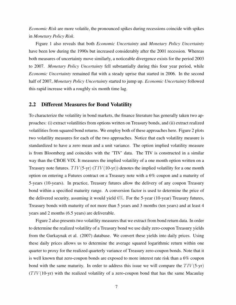
Economic Risk are more volatile, the pronounced spikes during recessions coincide with spikes

in Monetary Policy Risk.

Figure 1 also reveals that both Economic Uncertainty and Monetary Policy Uncertainty

have been low during the 1990s but increased considerably after the 2001 recession. Whereas

both measures of uncertainty move similarly, a noticeable divergence exists for the period 2003

to 2007. Monetary Policy Uncertainty fell substantially during this four year period, while

Economic Uncertainty remained flat with a steady uprise that started in 2006. In the second

half of 2007, Monetary Policy Uncertainty started to jump up. Economic Uncertainty followed

this rapid increase with a roughly six month time lag.

2.2 Different Measures for Bond Volatility

To characterize the volatility in bond markets, the finance literature has generally taken two ap-

proaches: (i) extract volatilities from options written on Treasury bonds, and (ii) extract realized

volatilities from squared bond returns. We employ both of these approaches here. Figure 2 plots

two volatility measures for each of the two approaches. Notice that each volatility measure is

standardized to have a zero mean and a unit variance. The option implied volatility measure

is from Bloomberg and coincides with the ’TIV’ data. The TIV is constructed in a similar

way than the CBOE VIX. It measures the implied volatility of a one month option written on a

Treasury note futures. TIV (5-yr) (TIV (10-yr)) denotes the implied volatility for a one month

option on entering a Futures contract on a Treasury note with a 6% coupon and a maturity of

5-years (10-years). In practice, Treasury futures allow the delivery of any coupon Treasury

bond within a specified maturity range. A conversion factor is used to determine the price of

the delivered security, assuming it would yield 6%. For the 5-year (10-year) Treasury futures,

Treasury bonds with maturity of not more than 5 years and 3 months (ten years) and at least 4

years and 2 months (6.5 years) are deliverable.

Figure 2 also presents two volatility measures that we extract from bond return data. In order

to determine the realized volatility of a Treasury bond we use daily zero-coupon Treasury yields

from the Gurkaynak et al. (2007) database. We convert these yields into daily prices. Using

these daily prices allows us to determine the average squared logarithmic return within one

quarter to proxy for the realized quarterly variance of Treasury zero-coupon bonds. Note that it

is well known that zero-coupon bonds are exposed to more interest rate risk than a 6% coupon

bond with the same maturity. In order to address this issue we will compare the TIV (5-yr)

(TIV (10-yr) with the realized volatility of a zero-coupon bond that has the same Macaulay

7

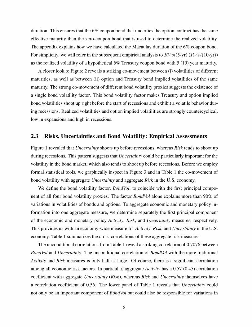
duration. This ensures that the 6% coupon bond that underlies the option contract has the same

effective maturity than the zero-coupon bond that is used to determine the realized volatility.

The appendix explains how we have calculated the Macaulay duration of the 6% coupon bond.

For simplicity, we will refer in the subsequent empirical analysis to RV ol(5-yr) (RV ol(10-yr))

as the realized volatility of a hypothetical 6% Treasury coupon bond with 5 (10) year maturity.

A closer look to Figure 2 reveals a striking co-movement between (i) volatilities of different

maturities, as well as between (ii) option and Treasury bond implied volatilities of the same

maturity. The strong co-movement of different bond volatility proxies suggests the existence of

a single bond volatility factor. This bond volatility factor makes Treasury and option implied

bond volatilities shoot up right before the start of recessions and exhibit a volatile behavior dur-

ing recessions. Realized volatilities and option implied volatilities are strongly countercyclical,

low in expansions and high in recessions.

2.3 Risks, Uncertainties and Bond Volatility: Empirical Assessments

Figure 1 revealed that Uncertainty shoots up before recessions, whereas Risk tends to shoot up

during recessions. This pattern suggests that Uncertainty could be particularly important for the

volatility in the bond market, which also tends to shoot up before recessions. Before we employ

formal statistical tools, we graphically inspect in Figure 3 and in Table 1 the co-movement of

bond volatility with aggregate Uncertainty and aggregate Risk in the U.S. economy.

We define the bond volatility factor, BondVol, to coincide with the first principal compo-

nent of all four bond volatility proxies. The factor BondVol alone explains more than 90% of

variations in volatilities of bonds and options. To aggregate economic and monetary policy in-

formation into one aggregate measure, we determine separately the first principal component

of the economic and monetary policy Activity, Risk, and Uncertainty measures, respectively.

This provides us with an economy-wide measure for Activity, Risk, and Uncertainty in the U.S.

economy. Table 1 summarizes the cross-correlations of these aggregate risk measures.

The unconditional correlations from Table 1 reveal a striking correlation of 0.7076 between

BondVol and Uncertainty. The unconditional correlation of BondVol with the more traditional

Activity and Risk measures is only half as large. Of course, there is a significant correlation

among all economic risk factors. In particular, aggregate Activity has a 0.57 (0.45) correlation

coefficient with aggregate Uncertainty (Risk), whereas Risk and Uncertainty themselves have

a correlation coefficient of 0.56. The lower panel of Table 1 reveals that Uncertainty could

not only be an important component of BondVol but could also be responsible for variations in

8

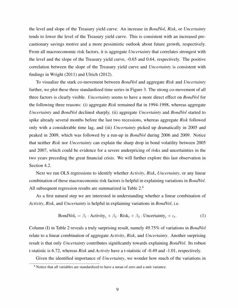
the level and slope of the Treasury yield curve. An increase in BondVol, Risk, or Uncertainty

tends to lower the level of the Treasury yield curve. This is consistent with an increased pre-

cautionary savings motive and a more pessimistic outlook about future growth, respectively.

From all macroeconomic risk factors, it is aggregate Uncertainty that correlates strongest with

the level and the slope of the Treasury yield curve, -0.65 and 0.64, respectively. The positive

correlation between the slope of the Treasury yield curve and Uncertainty is consistent with

findings in Wright (2011) and Ulrich (2012).

To visualize the stark co-movement between BondVol and aggregate Risk and Uncertainty

further, we plot these three standardized time series in Figure 3. The strong co-movement of all

three factors is clearly visible. Uncertainty seems to have a more direct effect on BondVol for

the following three reasons: (i) aggregate Risk remained flat in 1994-1998, whereas aggregate

Uncertainty and BondVol declined sharply, (ii) aggregate Uncertainty and BondVol started to

spike already several months before the last two recessions, whereas aggregate Risk followed

only with a considerable time lag, and (iii) Uncertainty picked up dramatically in 2005 and

peaked in 2009, which was followed by a run-up in BondVol during 2006 and 2009. Notice

that neither Risk nor Uncertainty can explain the sharp drop in bond volatility between 2005

and 2007, which could be evidence for a severe underpricing of risks and uncertainties in the

two years preceding the great financial crisis. We will further explore this last observation in

Section 4.2.

Next we run OLS regressions to identify whether Activity, Risk, Uncertainty, or any linear

combination of these macroeconomic risk factors is helpful in explaining variations in BondVol.

All subsequent regression results are summarized in Table 2.6

As a first natural step we are interested in understanding whether a linear combination of

Activity, Risk, and Uncertainty is helpful in explaining variations in BondVol, i.e.

BondVolt = β1 · Activityt + β2 · Riskt + β3 · Uncertaintyt + εt. (1)

Column (I) in Table 2 reveals a truly surprising result, namely 49.75% of variations in BondVol

relate to a linear combination of aggregate Activity, Risk, and Uncertainty. Another surprising

result is that only Uncertainty contributes significantly towards explaining BondVol. Its robust

t-statistic is 6.72, whereas Risk and Activity have a t-statistic of -0.49 and -1.01, respectively.

Given the identified importance of Uncertainty, we wonder how much of the variations in

6 Notice that all variables are standardized to have a mean of zero and a unit variance.

9

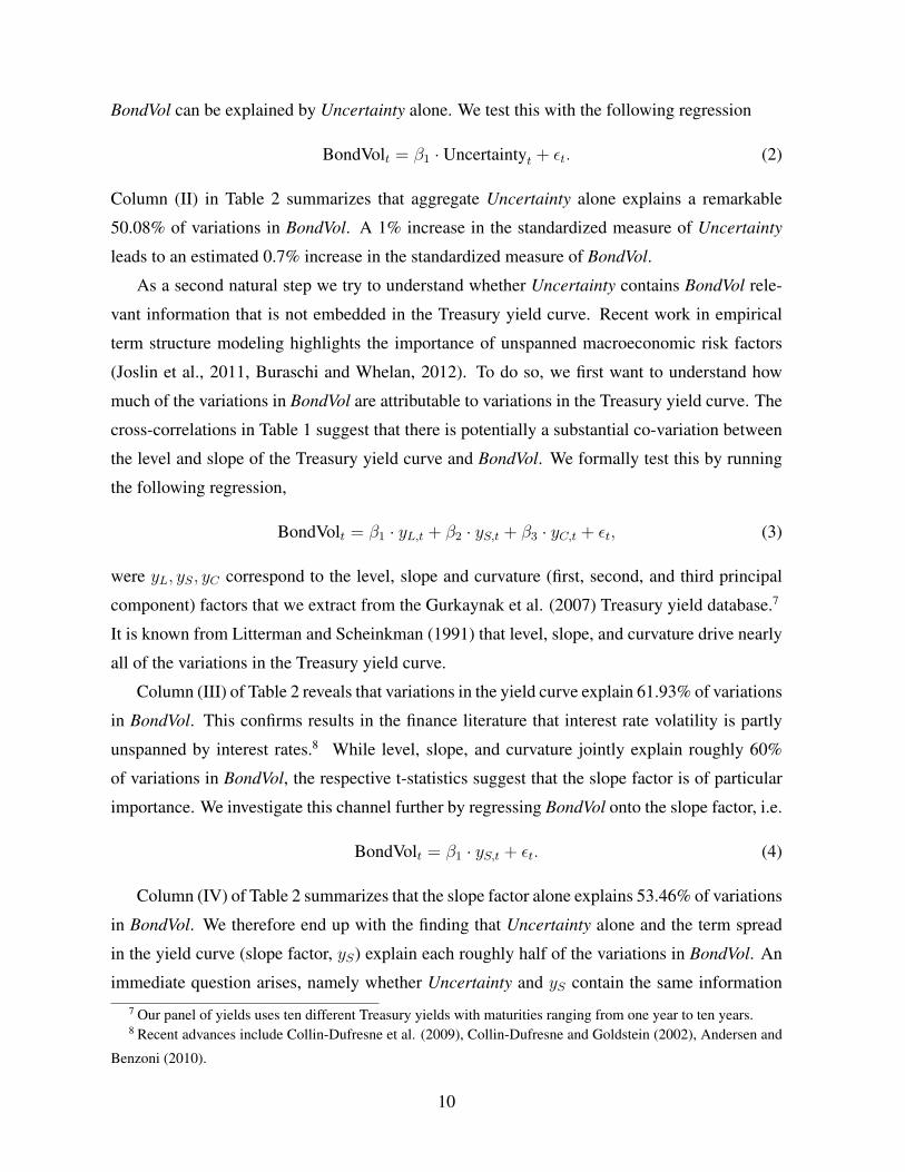
BondVol can be explained by Uncertainty alone. We test this with the following regression

BondVolt = β1 · Uncertaintyt + εt. (2)

Column (II) in Table 2 summarizes that aggregate Uncertainty alone explains a remarkable

50.08% of variations in BondVol. A 1% increase in the standardized measure of Uncertainty

leads to an estimated 0.7% increase in the standardized measure of BondVol.

As a second natural step we try to understand whether Uncertainty contains BondVol rele-

vant information that is not embedded in the Treasury yield curve. Recent work in empirical

term structure modeling highlights the importance of unspanned macroeconomic risk factors

(Joslin et al., 2011, Buraschi and Whelan, 2012). To do so, we first want to understand how

much of the variations in BondVol are attributable to variations in the Treasury yield curve. The

cross-correlations in Table 1 suggest that there is potentially a substantial co-variation between

the level and slope of the Treasury yield curve and BondVol. We formally test this by running

the following regression,

BondVolt = β1 · yL,t + β2 · yS,t + β3 · yC,t + εt, (3)

were yL, yS, yC correspond to the level, slope and curvature (first, second, and third principal

component) factors that we extract from the Gurkaynak et al. (2007) Treasury yield database.7

It is known from Litterman and Scheinkman (1991) that level, slope, and curvature drive nearly

all of the variations in the Treasury yield curve.

Column (III) of Table 2 reveals that variations in the yield curve explain 61.93% of variations

in BondVol. This confirms results in the finance literature that interest rate volatility is partly

unspanned by interest rates.8 While level, slope, and curvature jointly explain roughly 60%

of variations in BondVol, the respective t-statistics suggest that the slope factor is of particular

importance. We investigate this channel further by regressing BondVol onto the slope factor, i.e.

BondVolt = β1 · yS,t + εt. (4)

Column (IV) of Table 2 summarizes that the slope factor alone explains 53.46% of variations

in BondVol. We therefore end up with the finding that Uncertainty alone and the term spread

in the yield curve (slope factor, yS) explain each roughly half of the variations in BondVol. An

immediate question arises, namely whether Uncertainty and yS contain the same information7 Our panel of yields uses ten different Treasury yields with maturities ranging from one year to ten years.8 Recent advances include Collin-Dufresne et al. (2009), Collin-Dufresne and Goldstein (2002), Andersen and

Benzoni (2010).

10

or whether each of these factors carries its own BondVol relevant information. We approach

this problem from two angels. First, we regress Uncertainty on yS and jointly on [yL, yS, yC ]

to understand whether the yield curve spans all information embedded in Uncertainty. Second,

we take the unspanned part of Uncertainty and ask whether it adds explanatory power to the

regressions (4) and (3). The relevant regression output is summarized in Table 3.

With regard to the first analysis we find that 59% (48%) of variations in Uncertainty are

unspanned by yS ([yL, yS, yC ]). The term spread (yS) reveals the biggest amount of Uncer-

tainty related information (Ulrich (2012), Wright (2011)). Roughly half of the variations in

Uncertainty appear unspanned by the level, slope, and curvature. We denote Uncertainty\yS(Uncertainty\yL,yS ,yC) to be the component of aggregate Uncertainty that is orthogonal to yS([yL, yS, yC ]). To better understand the nature of Uncertainty and BondVol, we regress BondVol

on yield curve information and Uncertainty related information that is orthogonal to the yield

curve, i.e.

BondVolt = β1 · yS,t + β2 · Uncertaintyt,\yS + εt (5)

BondVolt = β1 · yL,t + β2 · yS,t + β3 · yC,t + β4 · Uncertaintyt,\yL,yS ,yC + εt. (6)

Table 4 summarizes the regression output and reveals that Uncertainty is not driven out by yield

curve information. All three principal components of the yield curve, as well as the unspanned

part of aggregate Uncertainty are significant contributors to BondVol. The term spread and the

unspanned part of uncertainty explain 62.57% of variations in BondVol, whereas level, slope,

and curvature together with the unspanned part of Uncertainty explain 70.77% of variations in

BondVol. We conclude that (i) Uncertainty is a very important macroeconomic risk factor for

BondVol that appears to be partly unspanned by the yield curve, and (ii) after controlling for

Uncertainty, traditional risk measures, such as Risk and Activity, do not help to explain varia-

tions in the volatility of the bond market. The unspanned nature of Uncertainty is consistent

with Duffee (2011) and Joslin et al. (2011) who emphasize the importance of incorporating un-

spanned macro risks into fixed-income models to better capture bond premiums. Whereas the

previous two papers focus on an empirical analysis and on bond premiums, we will show that a

parsimonious equilibrium model with Knightian uncertainty can very naturally endogenize that

Uncertainty should drive the volatility of interest rates.

We close the empirical examination with two last questions. First, which are the macroe-

conomic risk factors that even a parsimonious general equilibrium model should account for?

Second, do we have to account for a variance risk premium (VRP) in bond options?

11

With regard to the first closing question, Table 2 and Table 5 provide a striking message,

namely a parsimonious general equilibrium model for Treasury interest rates, interest rate

volatilities, and Treasury options should incorporate economic and monetary policy Activity

and Uncertainty measures, and ignore the Risk measures.

In particular, Table 2 revealed that Uncertainty explains roughly 50% of variations in the

volatility of bond prices and bond options, whereas Risk and Activity do not help to explain

variations in BondVol. A general equilibrium model derives also implications for the term

structure of interest rates. It is well known that the level factor explains more than 90% of

variations in the term structure of interest rates (Litterman and Scheinkman (1991)). Table 5

reveals that Activity and Uncertainty contribute significantly to variations in yL, whereas Risk

is negligible. Column (II) of Table 5 reveals that Economic Activity, Monetary Policy Activity,

Economic Uncertainty, and Monetary Policy Uncertainty explain jointly roughly 70% of vari-

ations in yL, whereas Economic Risk and Monetary Policy Risk have robust t-statistics of less

than 0.5. Monetary Policy Uncertainty has the highest absolute value of the robust t-statistic

(7.40), emphasizing its overall importance for the level (Table 5) and volatility (Table 2) of

interest rates. Wright (2011) and Ulrich (2012) explore the importance for the level and slope

of interest rates, whereas we analyze the importance for the volatility of interest rates and the

implication for bond options.

With regard to our second closing question, we wonder whether a parsimonious general

equilibrium model could abstract from the variance risk premium in bond options. The impor-

tance of the variance risk premium for predicting equity and Treasury excess returns is well

established in the literature.9 The focus of our paper is not on using option implied information

to predict excess returns but rather to endogenize the dynamic of BondVol with a parsimonious

equilibrium model. We document in Table 1 that interest rate volatilities have nearly identical

dynamics in the bond and in the option market. Intuitively, 91% of variations under the pricing

and under the physical probability measure are identical. The spread between both measures,

the VRP, accounts therefore only for a rather small portion of volatility. To aggregate informa-

tion, we determine the aggregate VRP as the first principal component of the spread between the

5-year (and 10-year) TIV 2 and the corresponding realized (physical) variance. Table 6 sum-

marizes that regressing the aggregate VRP measure jointly on Activity, Risk, and Uncertainty,

9 The importance of the variance risk premium for predicting equity returns has been documented in Bollerslev

et al. (2009) and Drechsler and Yaron (2011). The importance for predicting bond returns has been documented in

Mueller et al. (2011).

12

i.e.

VRPt = β1 · Activityt + β2 · Riskt + β3 · Uncertaintyt + εt, (7)

reveals that all macro and policy risks together explain only 5.51% of variations in the VRP

of bond options. Only Risk is weakly significant with a robust t-statistic of -2.1, whereas the

loadings on Activity and Uncertainty are not significant. The regression results are in line with

the literature, such as Mueller et al. (2011). The authors show that only disagreement about

prices of short-term bonds and disagreement about prices of long-term bonds, expressed as

dispersion of short-term and long-term interest rates, help to explain variations in the VRP

of bond options. The authors analog for our Risk and Uncertainty measures do not help to

explain the dynamic of the VRP in a statistically significant way. Buraschi and Whelan (2012)

endogenize disagreement about bond prices in a Bayesian model with heterogeneous agents

and informative signals and emphasize that disagreement about prices cannot easily arise in

a representative agent economy with Knightian uncertainty. Taking all of these observations

together motivates us to abstract from the VRP in our general equilibrium analysis to keep the

analysis parsimonious and to focus on first-order effects.

3 General Equilibrium Model with Endogenous Volatility

The findings in the previous section show that an increase in Uncertainty is strongly related

to an increase in the volatility of interest rates and bond options. It is an unresolved issue to

understand in a general equilibrium model why economic and monetary policy Uncertainty

matter so strongly for the volatility of the bond market. Ulrich (2012) explained why Monetary

Policy Uncertainty matters for the term spread but cannot explain its importance for the bond

option market. Drechsler (2012) calibrates a long-run risk model with Economic Uncertainty

to capture the variance risk premium in equity options, but does not address the issue of bond

market volatility or of Monetary Policy Uncertainty. Moreover, Drechsler (2012) shows that

equity options rely crucially on a variance risk premium, whereas we document that the variance

risk premium is of secondary importance for the dynamic of bond options. Buraschi and Whelan

(2012) and Xiong and Yan (2010) explain how Economic Uncertainty can affect interest rates

and bond premia, but leave unexplored how Monetary Policy Uncertainty affects bond options.

We now investigate whether a parsimonious macro-finance general equilibrium model with

Economic Activity, Monetary Policy Activity, Economic Uncertainty, and Monetary Policy Un-

certainty is able to match key features of the volatility in bond markets. To do so, we follow the

13

Knightian uncertainty literature by first introducing the agent’s most trusted belief about the data

DGP of Economic Activity and Monetary Policy Activity in the economy (benchmark model). In

a second step we will introduce that the agent has time-varying model misspecification doubts

about his most trusted benchmark model.

To simplify all mathematical derivations, we assume that (i) time is continuous, varying over

t ∈ [0, ...,∞), (ii) all Brownian motions are pairwise orthogonal, and (iii) the representative

agent has logarithmic preferences. We follow a standard procedure by assuming a complete

filtered probability space (Ω,F ,F, Q0), whereQ0 stands for the agent’s most trusted benchmark

DGP. Expectations under Q0 are denoted as E[.] instead of EQ0[.]. The analysis explains in

detail how the solution to the dynamic Gilboa and Schmeidler (1989) type min-max problem

determines endogenously the worst-case probability measure Qh.

3.1 Investor’s Most Trusted View on Monetary Policy and Real Growth

The goal of the model is to endogenize stochastic volatility in bond markets without relying on

what we called Risk in Section 2. The model will therefore rely on an homoscedastic endow-

ment economy with an agent who fears not to know the true DGP for Economic Activity and

Monetary Policy Activity. We do not aim to uncover why the agent fears to be confronted by

model misspecification doubts, but analyze its possible consequences for the volatility on bond

markets.

We model monetary policy and the real economy as exogenous processes and leave it to

future research to endogenize these processes. The agent believes that monetary policy controls

the trend growth rate, wt ∈ R, of inflation, d ln pt ∈ R. The agent understands that realized

inflation, d ln pt, is a noisy realization of the central bank’s intended rate of trend inflation, wt.

Inspired by our previous empirical analysis we denote wt to coincide with Monetary Policy Ac-

tivity. The real economy is characterized through the agent’s exogenous consumption growth

process, d ln ct ∈ R, whose trend growth rate, zt ∈ R, is time-varying. In analogy to our

previous empirical exercise we denote zt to capture Economic Activity. The agent believes that

Monetary Policy Activity can only in the short-run affect Economic Activity. We model this by

allowing for a non-zero correlation between Monetary Policy Activity shocks and Economic Ac-

tivity shocks. This non-zero correlation ensures long-run inflation neutrality, which is consistent

with a vertical long-run Philips curve.

The agent’s most trusted DGP of monetary policy actions and real growth can be conve-

14

niently described as: (d ln ct

d ln pt

)=

(c0 + zt

p0 + wt

)dt+

(σc 0

0 σp

)(dW c

t

dW pt

), (8)

where [c0, p0, σc, σp] ∈ R4+. Economic Activity and Monetary Policy Activity follow a zero-

mean Gaussian process(dzt

dwt

)=

(κzzt

κwwt

)dt+

(σ1z σ2z

0 σw

)(dW r

t

dWMPt

)(9)

with [−κz,−κw, σ1z, σw,−σ2z] ∈ R5+. The modeling of σ2z < 0 is consistent with recent

empirical macro-finance evidence in Piazzesi and Schneider (2006, 2010) and Ulrich (2012).

The investor has log utility with ρ characterizing his subjective time discount factor, i.e.

U(ct; zt) = Et

[∫ ∞t

e−ρs ln csds

]. (10)

3.2 Fear about DGP Misspecifications

The agent worries that theQ0 DGP for Economic Activity and Monetary Policy Activity in equa-

tion (9) is not correct. The true but unknown one-step ahead DGPs might differ by statistically

difficult to identify stochastic perturbations hrt , hMPt t. Each stochastic perturbation induces

a conditionally Gaussian Qh DGP for Economic Activity and Monetary Policy Activity, i.e.(dzt

dwt

)=

(κzzt

κwwt

)dt+

(σ1z σ2z

0 σw

)(dW r,h

t + hrtdt

dWMP,ht + hMP

t dt

). (11)

Notice that knowing the set of potentially correct one-step ahead perturbations (hrtdt, hMPt dtt)

is equivalent to knowing the set of potentially correct DGPs for Economic Activity and Monetary

Policy Activity.10

The agent observes central bank actions, which allows him to observe innovations in Mon-

etary Policy Activities, dWMPt . The policy relevant trouble with model misspecification doubts

is that the agent worries that dWMPt was not drawn from a mean zero Gaussian distribution,

but might indeed have come from a slightly perturbed density function. The magnitude of the

conditional one-step ahead perturbation is quantified through hMPt . Mathematically, this means

that the agent observes only

1

σw(dwt − κwwtdt) = dWMP,h

t dt+ hMPt dt, (12)

10 A formal proof is given in Chen and Epstein (2002).

15

where we will solve for hMPt dt as part of the min-max optimization problem below.

How is a rational agent going to cope with Knightian uncertainty about Monetary Policy

Activities? The answer is surprisingly intuitive, as he will surveil with highest scrutiny whether

there is statistical evidence that realized Monetary Policy Activity innovations were not drawn

from Q0 but instead from a perturbed density Qh. Mathematically, this allows for a convenient

characterization because the logarithmic likelihood ratio between a perturbed Gaussian one-

step ahead DGP and the most trusted (Gaussian) DGP for Monetary Policy Activity innovations,

dWMP , coincides with

lnLRMPt→t+dt := ln

Qh,WMP

t→t+dt

Q0,WMP

t→t+dt

= −1

2(hMP

t )2dt+ hMPt dWMP

t , (13)

where lnLRMPt→t+dt measures the amount of statistical (empirical) confidence that Monetary

Policy Activity is accurately described by a zero-mean Gaussian process.

The endogenous amount of model mistrust about future Monetary Policy Activities, lnLRMP ,

is an exponential martingale with stochastic volatility hMPt . This has the intuitive conse-

quence that the agent expects incoming Monetary Policy Activity innovations to confirm that

the most trusted DGP for Monetary Policy Activity (Q0) is indeed correct, i.e. Et[dQ0,WMP

t→t+dt ] >

Et[dQh,WMP

t→t+dt ]. If the set of potentially correct DGPs for future Monetary Policy Activities in-

creases (hMP increases), the endogenous heteroscedasticity in the agent’s confidence in Q0 will

increase. This implies that for each unit of unpredictable innovation in Monetary Policy Activ-

ity (dWMP ), the agent’s confidence in Q0 will vary more strongly over time. We show below

that this translates into stronger variations in the agent’s marginal utility per unit exposure to

dWMP .

After interpreting incoming Monetary Policy Activity innovations, the agent is able to infer

realized innovations in Economic Activity (dW r). For completeness, we also allow the agent to

have model misspecification doubts about the DGP of dW r. Mathematically, this means1

σ1z

(dzt − κzzt − σ2z(dW

MP,ht + hMP

t dt))

= dW r,ht + hrtdt (14)

is observed, but its decomposition is unobserved and the reason for Economic Uncertainty. Sim-

ilar to Knightian uncertainty about Monetary Policy Activities, the agent tries to learn through

likelihood ratio tests which DGP drives future Economic Activities. The logarithmic likelihood

ratio between the perturbed and the most trusted DGP for future Economic Activities, W rt , co-

incides with

lnLRrt→t+dt := ln

Qh,W r

t→t+dt

Q0,W r

t→t+dt= −1

2(hrt )

2dt+ hrtdWrt . (15)

16

We follow the research on dynamic recursive multiple priors, pioneered by Chen and Epstein

(2002) and Epstein and Schneider (2003), and assume the agent observes the set of potentially

correct economic and monetary policy one-step ahead perturbations hrtdt, hMPt dtt. Both

likelihood ratios, mentioned above, imply that observing the set of one-step ahead perturbations,

characterizes the set of potentially correct DGPs for both, Economic Activity and Monetary

Policy Activity. Mathematically, we constrain the amount of Economic Uncertainty and the

amount of Monetary Policy Uncertainty with the concept of multi-dimensional stochastic κ-

ignorance of Chen and Epstein (2002), i.e.

1

2(hit)

2dt ≤ Uncertit dt ∈ R+, ∀i ∈ r,MP. (16)

Notice that the amount of both uncertainties is observable and time-varying. We introduce

the time-variation by assuming that both uncertainties are driven by their own exogenous pro-

cesses that we denote as ηrt and ηMPt , respectively. Formally,

Uncertit dt :=(mi)2

2(ηit)

2dt, (17)

dηit = (aηi + κηiηit)dt+ σηi

√ηitdW

ηi

t , ∀i ∈ r,MP, (18)

with [mi, aηi ,−κηi , σηi ] ∈ R4+ ∀i ∈ r,MP. Note that the scaling parameters mi ∀i ∈

r,MP govern the absolute magnitude of Uncertit, whereas the time series behavior is gov-

erned by ηit. The heteroscedasticity in the amount of Economic Uncertainty (ηrt ) and Monetary

Policy Uncertainty (ηMPt ), makes the set of potentially correct DGPs heteroscedastic and will

endogenously create stochastic volatility in the agent’s stochastic discount factor and in the

equilibrium bond and option market.

3.3 Optimization Problem and Endogenous Characterization of Qh

The investor has min-max preferences and searches within the set of potentially correct DGPs

for the unique economic and monetary policy Activity DGP that minimizes his expected life-

time utility. Formally, the investor solves

minh∈hrt , hMP

t tEh

[∫ ∞t

e−ρ(s−t) ln csds|Ft]

(19)

s.t.(8), (11), (16), (17), (18). (20)

17

The solution to the minimization problem follows Chen and Epstein (2002) and is summarized

in the following proposition.11

Proposition 1

The data generating process for Economic Activity and Monetary Policy Activity that min-

imizes the agent’s expected life-time utility is characterized by the following one-step ahead

perturbations

hr(t) = −√

2 · Uncertrt ∈ R− (21)

hMP (t) =

√2 · UncertMP

t ∈ R+. (22)

The proof of Proposition 1 is in the appendix.

Proposition 1 suggests that the ambiguity averse investor does portfolio and asset pricing

decisions, assuming that Economic Activity and Monetary Policy Activity are affected by the

worst-case one-step ahead perturbations, hrt , hMPt . Notice that these perturbations could indeed

characterize the true but unknown DGP of Economic Activity and Monetary Policy Activity. To

save notation, we will from now on refer to hrtdt and hMPt dt as the optimally chosen one-step

ahead equilibrium distortions.

Another intuitive insight from Proposition 1 is that periods of increased Monetary Policy

Uncertainty (Economic Uncertainty) are periods where the representative agent’s subjective

forecast of future Monetary Policy Activity (Economic Activity) deviates more strongly from the

most trusted Q0 benchmark forecast. Finally, the endogenously chosen (worst-case) one-step

ahead belief perturbations hrtdt and hMPt dt for anticipated future economic and monetary policy

Activity introduce stochastic volatility into the agent’s marginal rate of substitution.

3.4 Endogenous Marginal Rate of Substitution

The ambiguity averse investor evaluates his expected life-time utility under the worst-case DGP,

i.e.

Uh(c0; z0, ηr0, η

MP0 ) = Eh

0

[∫ ∞0

e−ρt ln ctdt

], (23)

11 Other applications of Chen and Epstein (2002) include Sbuelz and Trojani (2002, 2008), Drechsler (2012),

and Ulrich (2012), among others.

18

where z0, ηr0, η

MP0 emphasize the dependence on the revealed amount of Knightian uncertainty.

From an econometric point of view it is beneficial to re-write the agent’s expected life-time

utility under Q0, because Q0 is the agent’s most trusted DGP for the economy and therefore the

most likely description of how the exogenous processes of the economy move in the data.

Applying the Radon Nikodym derivative allows us to re-write the agent’s worst-case ex-

pected life-time utility under Q0, i.e.

Uh(c0; z0, ηr0, η

MP0 ) = E0

[∫ ∞0

LRr0→t · LRMP

0→t · e−ρt ln ctdt

](24)

d(LRr

t→t+dt · LRMPt→t+dt

)LRr

t→t+dt · LRMPt→t+dt

= −√

2 · Uncertrt · dW rt +

√2 · UncertMP

t · dWMPt . (25)

The product of both marginal likelihood ratios coincides with the accumulated amount of

confidence in the accuracy ofQ0 for predicting future economic and policy actions. Hansen and

Sargent (2008) recommend to interpret this confidence measure as an endogenously constrained

preference shock. The endogenous preference shock has no equilibrium asset pricing effects if

the investor has 100% confidence in Q0. This occurs if realized data on Economic Activity

and Monetary Policy Activity confirm that Q0 is the single most reliable forecasting DGP (i.e.

lnLRr · lnLRMP 0). On the other hand, this endogenous preference shock has severe asset

pricing implications in periods where the agent is confronted with sufficient doubt thatQ0 might

be incorrect.

Suppose the agent observes an unpredictable reduction in Economic Activity (i.e. dW r < 0).

As an endogenous response, the investor’s doubt about the accuracy of the AR(1) assumption

for Economic Activity increases, because the worst-case (but still potentially correct) DGP for

Economic Activity predicted a negative innovation in dW r. This is intuitive because since the

DGP for Economic Activity is not known, a realized value for Economic Activity that is lower

than forecasted under the AR(1) specification (Q0), i.e. zt+dt < Et[dzt], increases the observed

statistical evidence that the worst-case DGP might indeed be correct. News about lower than

expected Economic Activity hurts a min-max preference investor twice. First, the investor is in

a state of low consumption growth and second, the investor is confronted with more statistical

evidence that his trusted Q0 DGP for Economic Activity is too optimistic.

Conversely, suppose the agent observes an unpredictable increase in Monetary Policy Ac-

tivity (trend inflation), i.e. dWMP > 0. In equilibrium, this increases the agent’s fear that

his trusted Q0 forecast for future Monetary Policy Activity might be systematically downward

biased. Because of σ2z < 0 this implies that forecasts for Economic Activity might be too

optimistic under Q0.

19

The endogenous intertemporal marginal rate of substitution (MRS), m, accounts for the

standard logarithmic utility consumption risk kernel and for model misspecification doubts,

which are driven by shocks to Economic Activity and shocks to Monetary Policy Activity. Note

that it is somewhat surprising that although m is an endogenous equilibrium outcome of the

dynamic min-max optimization problem in Proposition 1, its equilibrium characterization is

quite tractable, i.e.

mt,t+∆ = e−ρ∆ ·(ct+∆

ct

)−1

· LRrt→t+∆ · LRMP

t→t+∆. (26)

The equilibrium MRS of a min-max agent accounts not only for the standard consumption risk

kernel, but also for a Knightian uncertainty kernel (Chen and Epstein, 2002, Ulrich, 2012). The

Knightian uncertainty kernel captures the time-varying confidence in the accuracy of the most

trusted Q0 forecast for future Economic Activities and future Monetary Policy Activities. It is

an intuitive learning point that the endogenous innovations in the uncertainty kernel coincide

with innovations in Economic Activity and innovations in Monetary Policy Activity. Stochastic

volatility in the accumulated amount of model misspecification doubts leads to a heteroscedas-

tic MRS. Notice that this result holds independent of whether or not consumption itself is het-

eroscedastic.

It is worth emphasizing that exposure to Knightian uncertainty about Economic Activity and

about Monetary Policy Activity endogenizes two stochastic market prices of Knightian uncer-

tainty. The dynamic of the MRS reveals this property immediately, i.e.

−dmt

mt

= ρdt+dctct−d(LRr

t→t+dt · LRMPt→t+dt

)LRr

t→t+dt · LRMPt→t+dt

= ρdt+dctct

+√

2 · Uncertrt · dW rt −

√2 · UncertMP

t · dWMPt . (27)

The market price of consumption risk is constant and positive, i.e. σc > 0. On the contrary,

the market price for exposure to Knightian uncertainty about Economic Activity is positive and

time-varying, i.e.√

2 · Uncertrt ∈ R+. Equity would pay off a positive equity risk premium

because of its positive exposure to Economic Activity (Bansal and Yaron, 2004). On the other

hand, Knightian uncertainty about future Monetary Policy Activities pays out a negative but

also time-varying market price of uncertainty, −√

2 · UncertMPt ∈ R−. An asset whose re-

turn has negative exposure to Monetary Policy Activity shocks would pay a positive equilibrium

premium. In Ulrich (2012) this makes nominal Treasury bonds pay out a positive premium,

whereas in Ang and Ulrich (2012) this would make equity pay out a positive equity risk pre-

mium.

20

3.5 Endogenous Stochastic Volatility in Marginal Rate of Substitution

We emphasize the empirical puzzle from Section 2, namely that from a variety of traditional

macro risk factors it has been only Uncertainty which explained a considerable fraction of

variations in the volatility of bonds and bond options. In this section we analyze whether our

simple general equilibrium model is able to endogenize the same insight.

To investigate the volatility implications further, we want to understand how Uncertainty

affects the conditional variance of the agent’s MRS. The previous equation implies that the

conditional variance of the logarithmic MRS is affine in the time-varying amount of Monetary

Policy Uncertainty and Economic Uncertainty, i.e.

V art (d lnmt) = σ2cdt+ 2 ·

(Uncertrt + UncertMP

t

)dt. (28)

The effect of economic and monetary policy uncertainty on the variance of the agent’s MRS

is clearly visible from the last equation. Two observations are worth mentioning. First, an

exogenous rise in either Economic Uncertainty or Monetary Policy Uncertainty leads to an

endogenous increase in the conditional variance of the agent’s MRS. A one percent increase in

either of these uncertainties leads to an economically meaningful 2% increase in V art(d lnmt).

Variations in Uncertainty could therefore indeed be potentially very important for understanding

variations in the volatility of financial markets.

Second, the equilibrium outcome for V art(d lnmt) emphasizes that heteroscedasticity in

the agent’s MRS might arise from variations in the agent’s confidence in the accuracy of his

most trusted workhorse DGP. These fluctuations might have nothing to do with fluctuations

in standard measures of fundamental macro Risk or fundamental macro Activity. An observer,

who stands outside of the model (ignoring Knightian uncertainty) would be tempted to term this

excess volatility. To be more precise, the economic policy uncertainty factors that drive in our

model the volatility in the financial market are of course related to the underlying macro econ-

omy, but variations in these factors (ηr and ηMP ) are not captured by standard fundamental risk

factors, such as business cycle risk or macroeconomic volatility risk. Instead, a model must be

extended to e.g. Knightian uncertainty, to account for this feature of the data. Patton and Tim-

mermann (2010) conclude in their extended empirical analysis of macroeconomic dispersion

data that Knightian uncertainty could indeed be the economic reason for time variation in ηr

and ηMP . Our economy takes this insight as an exogenous input and shows that the endogenous

implications for the volatility of the agent’s MRS could be potentially substantial.

21

3.6 Endogenous Bond Market Volatility

The previous section showed that economic policy Uncertainty drives variations in the con-

ditional variance of the agent’s MRS. This has the intuitive equilibrium implication that the

volatility of all financial assets loads on Uncertainty. To further illustrate this observation, we

will focus on the volatility of Treasury bonds and bond options and leave it to future research

to extend the model to equity options.

Let Nt(τ) denote the equilibrium price at time t of a τ maturity zero-coupon Treasury bond.

It is well known that the price of such a bond satisfies the following Euler equation

Nt(τ) = Et

[mt,t+τ

ptpt+τ

$1

]. (29)

We verify in the appendix thatNt(τ) is exponentially affine in four macroeconomic risk fac-

tors, namely, (i) Economic Activity, (ii) Monetary Policy Activity, (iii) Economic Uncertainty,

and (iv) Monetary Policy Uncertainty. The activity factors enter the price of Treasury bonds be-

cause they affect the agent’s inference about future economic growth and about future inflation.

Both uncertainty factors enter as endogenous uncertainty premiums into the equilibrium price

of bonds, i.e.

Nt(τ) = eA(τ)+Bz(τ)·zt+Bw(τ)·wt−Bhr (τ)·√

2·Uncertrt+BhMP (τ)·√

2·UncertMPt , (30)

where the loadings A(τ) and B(τ) are deterministic functions of the underlying economy and

fully characterized in the appendix.12

In order to prepare for the upcoming maximum likelihood estimation of the general equilib-

rium model we solve explicitly for the continuously compounded yield of zero-coupon Treasury

bonds. We denote these yields as yt(τ) = − 1τ

lnNt(τ), i.e.

yt(τ) = a(τ) + bz(τ) · zt + bw(τ) · wt − bhr(τ) ·√

2 · Uncertrt + bhMP (τ) ·√

2 · UncertMPt ,

(31)

where a(τ) = −A(τ)τ

and b(τ) = −B(τ)τ

.

Notice that the type of Uncertainty matters. Suppose there is an exogenous increase in

Economic Uncertainty. This leads to an endogenous increase in the market price of Economic

Uncertainty, because the min-max agent worries that future Economic Activity might be sys-

tematically lower than previously expected. Investing into Treasury bonds becomes a more

12 Note that one can substitute into the last equation the equilibrium relationship: hrt = −√

2 · Uncertrt and

hMPt =

√2 · UncertMP

t .

22

valuable investment strategy because being long a Treasury bond hedges bad realizations of

Economic Activity. A min-max agent hedges the rise in Economic Uncertainty through an in-

creased demand for Treasury bonds. The price of these bonds increases because the negative

Economic Uncertainty premium in Treasury bonds increases in absolute magnitude to keep

Treasury bonds in zero net supply. The increase in the price of a Treasury bond is consistent

with a flight to safety and leads to a steepening of the Treasury yield curve in times of elevated

Economic Uncertainty. The yield curve steepens because the impact of the Economic Uncer-

tainty shock is expected to mean revert back to zero, which implies a relatively strong reduction

of short-term Treasury yields and a minor reduction in long-term yields.

On the other hand, suppose there is an exogenous increase in Monetary Policy Uncertainty.

The negative market price of Monetary Policy Uncertainty increases in magnitude (Proposition

1), because the min-max agent worries to systematically under-predict future inflation. The

monetary uncertainties associated with investing into Treasury bonds increase because the real

payoff of these bonds is worse than expected in periods where realized trend inflation is higher

than predicted. Since Treasury bonds do not hedge the amplified amount of Monetary Policy

Uncertainty the price of these bonds drops because the positive Monetary Policy Uncertainty

premium in Treasury bonds increases to keep the Treasury bonds in zero net supply. The result-

ing Monetary Policy Uncertainty premium increases all Treasury yields and leads to an upward

sloping yield curve if innovations to Monetary Policy Activities are sufficiently persistent.

Knowing how economic and monetary policy measures for Activity and Uncertainty drive

the price of Treasury bonds, allows us to determine the conditional variance of bond returns

(quadratic variation in instantaneous bond returns). We denote this instantaneous return vari-

ance of a τ maturity Treasury bond as RV art(Nt(τ)) to emphasize its close relation to the

realized volatility measure in Section 2, i.e.

RV art(Nt(τ)) = (Bw(τ) · σw +Bz(τ) · σ2z)2 +B2

z (τ) · σ21z

+B2hr(τ) · σ2

ηr · (mr)2 · ηrt +B2hMP (τ) · σ2

ηMP · (mMP )2 · ηMPt , (32)

where the B(τ) loadings coincide with the corresponding loadings from the price of the bond.

Consistent with empirical evidence in Section 2, we see that only aggregate Uncertainty

drives the realized variance of Treasury bond returns. A positive shock to either type of Uncer-

tainty leads to an endogenous increase in the variance of bond returns. This happens because an

increase in Uncertainty increases not only the discount rates (market price of uncertainty) but

it also increases the conditional variance of the agent’s MRS, which increases the conditional

variance of bond returns.

23

We now want to use the equilibrium insights to better understand the empirical observation

from Section 2. We uncovered that most of the variations in option implied bond volatilities

arise from variations in the realized volatility of bond returns. A more skill-full expression for

this observation is that we want to understand why bond volatilities move similarly under the

physical and under the pricing probability measure. We deliberately abstract from a variance

risk premium (see discussion in Section 2) which as a consequence generates the high covari-

ation between the physical and the pricing dynamic of volatility. An analytically convenient

consequence of this modeling choice is that the option implied variance on a bond coincides

with the expected variance of the bond return (under the physical probability Q0), i.e.

Et [RV art+m(Nt+m(τ))] = (Bw(τ) · σw +Bz(τ) · σ2z)2 +B2

z (τ) · σ21z+

+∑

i∈r,MP

B2hi(τ) · σ2

ηi ·mi ·[(mi · ηit +

aηi ·mi

κηi

)· eκηi ·m −

aηi ·mi

κηi

].

(33)

The m-period ahead variance forecast of a τ period Treasury bond coincides in the model with

the m-period option implied variance of a τ maturity Treasury bond. The option implied bond

volatility is time-varying and increases in periods where economic and/or monetary policy un-

certainty rises. The model explains naturally why an elevated amount of economic and mone-

tary policy Uncertainty leads to an increase in the price of bond options. The persistence of both

types of Uncertainty, i.e. κηr and κηMP and the scaling parameter mr and mMP , determine how

strongly both uncertainties affect bond options. The persistence of both uncertainties is pinned

down through the time-series of ηr and ηMP , whereas the magnitude of both scaling parameters

must be identified through a structural model estimation.

4 Structural Estimation of General Equilibrium Model

The previous section showed that Knightian uncertainty about Monetary Policy Activity and

Economic Activity is indeed able to endogenize the empirical bond volatility pattern that we

document in Section 2 of this paper. As a last insight we would like to use the equilibrium

model to understand whether Economic Uncertainty and Monetary Policy Uncertainty affect

yields and volatilities the same way or whether there are meaningful differences. To do so, we

estimate the model with the following data, which are laid out in more detail in the appendix.

First, we use continuously compounded yields on Treasury zero-coupon bonds with matu-

rities of 1, 2, 3, 4, 5, 6, 7, 8, 9, and 10 years. The data is taken from the Gurkaynak et al. (2007)

24

database and comprises the years 1972:Q1 to 2009:Q2. Second, we use all four bond volatility

measures that were introduced in Section 2. In short, these were realized quarterly volatility of

the 4.5-year and the 6.5-year zero-coupon Treasury bond, as well as the option implied volatility

on the 5-year and on the 10-year Treasury note. The option implied volatility coincides with the

TIV series in Bloomberg. All four volatility time series start in 1994:Q1, which is the earliest

date for which we have access to all four volatility measures.

Third, we use two macroeconomic measurement equations to identify d ln ct and d ln pt.

We match the former with realized quarterly GDP growth and the latter with the GDP implicit

inflation rate. The FRED database from the St. Louis Federal Reserve publishes both time

series. Fourth, our four, in real-time observable, state equations coincide with the Activity

and Uncertainty measures from Section 2. In summary, these are (i) Economic Activity (zt),

(ii) Monetary Policy Activity (wt), (iii) Economic Uncertainty (ηrt ), and (iv) Monetary Policy

Uncertainty (ηMPt ). This data is from 1972:Q1 to 2009:Q2. The estimation starts in 1972:Q1

because of the real-time survey data that we rely upon to construct the four state equations.

We use maximum likelihood to estimate the model. Four observable and conditionally

Gaussian state variables are employed to fit 16 measurement equations. We summarize the

parameters of the economy in a vector θ and all four state equations in a vector st. The appendix

verifies that the joint logarithmic likelihood function, lnL(θ), coincides with

lnL(θ) =T−1∑t=1

ln fm(mt+1|zt, wt; θ) + ln fs(st+1|st; θ)

+ ln fuy(uyt,τ |st; θ) + ln fuRVol(uRVol

t,τ |ηMPt , ηrt ; θ) + ln fuTIV(uTIV

t,τ |ηMPt , ηrt ; θ)

(34)

where all the marginal transition densities, fm, fs, fuy , fuRV ol , fuTIV are fully characterized in

the appendix. The marginal density fm captures the joint likelihood of d ln ct and d ln pt, fs cap-

tures the joint likelihood of the four state processes, fuy stands for the joint likelihood of the ten

Treasury yields, fuRV ol stands for the joint likelihood of the two realized bond volatilities, and

last but not least, fuTIV , captures the joint likelihood of the two option implied bond volatilities.

The empirical fit of the model is surprisingly good, considering that (i) it only uses four

observable state processes, (ii) it matches Treasury yields and Treasury volatilities, and (iii)

it matches option implied bond volatilities with a zero variance risk premium. How does the

model achieve that? The empirical insights of Section 2 helped to identify economic and mone-

tary policy Activity and Uncertainty as the key macro risk factors. Moreover, Section 2 identified

that the dynamic of the sample variance risk premium is negligible.

25

4.1 Cross-Section of Bond Volatility

Figure 5 plots the estimated model implied term structure of bond volatilities and option volatil-

ities together with the data counterpart and standard error bounds. The upper left panel shows

that the average fit to the physical bond volatility is very accurate. The annualized physical

volatility of the 4.5-year zero-coupon bond is roughly 4%, whereas it is roughly 6% for the

6.5-year zero-coupon bond. Notice that we explained in Section 2 that we do not compare the

5 (10)-year TIV with the physical volatility of the 5 (10)-year zero-coupon Treasury volatility,

but that instead we match their effective duration, as laid out in the Appendix. The upper right

panel shows that the model is indeed able to explain the term structure of option implied volatil-

ities with only Uncertainty and with a zero variance risk premium. The lower left and the lower

right panel plot the model implied term structure for physical bond volatilities and option im-

plied volatilities, for the period 1972:Q1 to 2009:Q2. Both term structures are strongly upward

sloping with a similar shape to the 1994 to 2009 data.

Figure 6 shows that the fit to the yield curve is successful. The model implied yield curve

is clearly upward sloping and all yields are within standard confidence error bounds. The fit to

the 4.5 and 6.5-year yield is actually very good, which is comforting because we also match the

4.5 and the 6.5-year interest rate volatility and the corresponding option implied volatility.

The parameter estimates in Table 7 reveal that the yield curve model is effectively a two-

factor model, whereas the volatility model is effectively a one-factor model. The very persistent

Monetary Policy Activity measure, is known to be the most important observable macroeco-

nomic yield curve factor (Ulrich, 2012, Ang and Ulrich, 2012). Our estimation confirms that

and stresses that Monetary Policy Uncertainty is an important volatility factor.

It is interesting to note that if one considers Uncertainty to be an aggregate macro factor

with two subcomponents, our estimation argues that Economic Uncertainty is the high fre-

quency uncertainty component, whereas Monetary Policy Uncertainty is the lower frequency

component. The half-life of a shock to Monetary Policy Uncertainty is over 50 years. This is

a potentially alarming finding for policy makers because it indicates that increases in Monetary

Policy Uncertainty are extremely long lasting.

4.2 Bond Volatility and Monetary Policy Uncertainty

We next turn to the question whether the model provides any insights to why volatility, as docu-

mented in Section 2, appears to be underpriced in 2004 to 2007. Figure 7 plots physical volatil-

26

ity (top panel), option implied volatility (middle panel), and the corresponding Treasury yield

(lower panel) for the 4.5-year Macaulay duration bond (left panels) and the 6.5-year Macaulay

duration bond (right panels). The physical bond volatility moves very closely to the priced

volatility, for all maturities, as already noted in Section 2.

Three volatility related observations are worth mentioning. First, physical and priced volatility

increase sharply right before recessions. The model captures this stylized fact accurately. That

is a striking observation because (i) the model implied volatilities are mainly driven by Mon-

etary Policy Uncertainty, and (ii) it emphasizes that spikes in option implied bond volatility

seems to arise from spikes in physical volatility.

Second, a strong divergence in model implied and data observed volatility starts in 2004 and

lasts until the middle of 2007. With the help of the model we can infer that the understatement

of physical bond volatility was then transferred into lower option volatilities. Both volatility

markets were affected. So it was not that the market price of volatility risk was too low, instead

the estimated amount of volatility risk was too low, compared to the amount of Monetary Policy

Uncertainty in the U.S. economy. The under-prediction of volatility was sharply reversed in late

2007, when the financial crisis started to arrive. The sudden increase in fear is apparent because

physical and priced volatility started to overshoot the model counterpart.

Third, for the moment it remains a puzzle why physical volatility started to drop signifi-

cantly in 2004, compared to the observed amount of Monetary Policy Uncertainty. Even more

puzzling is the observation that the ’artificially low’ Treasury yields (according to our model)

after the 2001 recession, started to revert back to fundamentals (our model) in 2004. There is a

striking negative correlation between the yields coming back to fundamentals and the volatility

deviating from fundamentals. In other words, the Federal Reserve started to raise interest rates

in 2004 to correct the path of easy monetary policy after 2001, which the volatility market in-

terpreted as a signal towards lower financial market risk ahead. But according to our model, the

amount of Monetary Policy Uncertainty remained unchanged which should have led volatility

in the bond market to remain unchanged. The market noticed the underpricing of risk when the

financial crisis hit unexpectedly and when monetary policy prepared for the launch of untested

Quantitative Easing policies.

When the financial crisis hit in late 2007, the Federal Reserve went back to the policy of

easy money, which in our estimation is clearly visible, because even long-term rates started to

be again substantially lower than what our model with Economic Activity and Monetary Pol-

icy Activity justifies. At the same time, volatility in the market starts to overshoot compared

27

to the amount of Monetary Policy Uncertainty in the economy. This indicates a complex in-

teraction between actions of the Federal Reserve and the volatility of bond markets which our

consumption-based asset pricing model captures partly. We leave it to future research to further

analyze this identified puzzle.

Figure 8 shows that the term structure of volatility in the bond and in the option market was

noticeably higher during the Monetary Policy Experimentation than during the Great Moder-

ation. The model has been estimated for the entire sample and sample averages are used to

find the term structure for these subperiods. The longer the duration of the underlying Treasury

bond, the higher the volatility spread. The average bond volatility for a 10-year Macaulay dura-

tion bond has been 10.72% during the Monetary Policy Experimentation and 8.35% during the

Great Moderation. The corresponding average option implied volatility has been 11.09% dur-

ing the Monetary Policy Experimentation and 8.83% during the Great Moderation. Notice that

these volatility spreads arise because of variations in the observed amount of Monetary Policy

Uncertainty.

A variance decomposition of the model implied bond and option implied volatility reveals

that the main uncertainty driver of bond volatility is Monetary Policy Uncertainty. The intuition

for this model implication is very instructive. Fear about under-predicting future Monetary

Policy Activity leads to an upward sloping nominal yield curve (Ulrich, 2012), whereas we

find in this paper that fear about over-predicting future Economic Activity leads to a downward

sloping nominal yield curve. It is a stylized empirical fact that the U.S. Treasury yield curve

is on average upward sloping. Monetary Policy Uncertainty endogenizes this stylized fact and

makes the bond volatility be time-varying. Economic Uncertainty can endogenize time-varying

volatility as well, but at the cost of a downward sloping Treasury yield curve. We match in our

structural model estimation both, the dynamics of the Treasury yield curve and the dynamics

of the volatility in bond and option markets. In retrospect it is therefore not a surprise that

Monetary Policy Uncertainty dominates Economic Uncertainty.

The dominance of Monetary Policy Uncertainty for the volatility of bond options is depicted

in Figure 9. It plots the time series for the model implied volatility on a one month option

written on a 10-year Treasury note together with our observable measure of Monetary Policy

Uncertainty. The unconditional correlation of 99% confirms that Monetary Policy Uncertainty

is the main driver in the model for the volatility of bond and bond option markets. Periods of

spikes in Monetary Policy Uncertainty, such as the 1981, 1991, and 2008 recessions are periods

where the volatility of options spike as well.

28

We plot in Figure 10 several financial market responses to a one standard deviation shock

to ηMPt . This figure reveals that shocks to Monetary Policy Uncertainty have a severe effect

on the financial market. The slope of the yield curve would increase by 0.2% as the monetary

policy ambiguity premium steepens (Ulrich, 2012, Wright 2011). The steepening of the yield

curve is accompanied by a 4.74% increase in the physical volatility of a 4.5-year Macaulay

duration bond, and a 5.99% increase in the physical volatility of a 6.5-year Macaulay duration

bond. Option implied volatilities on bonds with the same Macaulay duration would increase

by the same amount because we abstract from a variance risk premium (see Section 2).13 The

estimated high persistence of ηMP makes the impact on the slope and the volatility of interest

rates to be long lasting.

4.3 Detection Error Probability

One natural question of interest remains: how much Knightian uncertainty has been necessary

to endogenize the above mentioned equilibrium results? The appendix derives the analytical ex-

pression for the detection error probability (DEP). Detection error probabilities are an intuitive

tool, because they quantify the probability that an econometrician could, after seeing the entire

sample of the state vector, tell whether Q0 or Qh generated the data. Notice that two Gaussian

transition densities are indistinguishable if their DEP is 50%. According to Hansen and Sargent

(2008) a DEP of 10% or more poses a realistic threat of choosing the wrong state vector DGP.

Our maximum likelihood estimation implies a DEP of 21.65%. This says that there is

a 21.65% chance that an econometrician chooses the wrong DGP for Economic Activity and

Monetary Policy Activity, after seeing the entire state vector. This implies that the agent has

been confronted with a lot of Knightian uncertainty about whether or not Q0 or Qh generated

the observed economic and policy data.

5 Conclusion

Our analysis started out documenting that roughly half of the quarterly variations in option

implied bond volatilities and interest rate volatilities correlate with real-time measures of eco-

nomic and monetary policy uncertainty. Standard measures of macroeconomic volatility and

business cycle risk did not contribute to explain variations in those bond volatilities.

13 The result would also hold in a model with a non-zero variance risk premium that is driven by a factor different

than Monetary Policy Uncertainty.

29

We propose a simple and extremely parsimonious general equilibrium asset pricing model

that is able to explain why economic and monetary policy uncertainty matter so strongly for the

volatility of bond and option markets. Estimating the equilibrium model with maximum likeli-

hood reveals that Monetary Policy Uncertainty is the most important macroeconomic volatility

risk factor in bond markets. A one standard deviation shock to Monetary Policy Uncertainty

increases the slope of the yield curve by 0.2% and raises the (physical) volatility and option im-

plied (priced) volatility of a 6.5-year Macaulay duration bond by an economically meaningful

6%.

We conclude first, that volatility in bond markets suggests that Knightian uncertainty is far

more important that traditional measures of volatility risk and expected business cycle risk.

Second, a simple general equilibrium asset pricing model with only observable risk factors can

account for the key dynamics in the cross-section and time-series of Treasury interest rates,

interest rate volatility, and option implied volatility. We leave an extension towards equity

options and towards analyzing the variance risk premium to future research.

30

6 Appendix

”For Online Publication”

6.1 Macaulay Duration for Matching Interest Rate Risk

The underlying contract of a TIV (5−yr) (TIV (10−yr)) is a 6% Treasury coupon bond with not more

than 5 years and 3 months (ten years) and at least 4 years and 2 months (6.5 years) time to maturity. We

use the following approximation to match the TIV implied volatility to the volatility of an option on a

zero-coupon bond.

First, the coupon rate of the underlying is fixed to be 6%. Second, as the maturity of the deliverable

claim, we use the average of 4 and 5 years for the TIV(5-yr) (i.e. 4.5) and the average of 6 and 10 years

for the TIV(10-yr) (i.e. 8). Third, the time span of the option data is 1994:Q1 to 2009:Q2. The average 8

year (4.5) Treasury yield has been 5% (4.6%) during this time period. Fourth, the Macaulay duration of

a Treasury note with 6% coupon, maturity in 8 years, which trades at a yield of 5% is approximately 6.5.

Analogously, the Macaulay duration of a Treasury note with 6% coupon, maturity in 4.5 years, which

trades at a a yield of 4.6% is approximately 4.5.

To summarize, the underlying of a TIV(5-yr) and TIV(10-yr) contract has had approximately the

same interest rate risk in 1994:Q1 to 2009:Q2 than a 4.5-yr and 6.5-yr Treasury zero-coupon bond,

respectively.

6.2 Data

State Variables

We use real-time forecast data from the Survey of Professional Forecasters to identify the empirical

counterpart of wt, zt, ηMPt , ηrt . We match wt (zt) with the demeaned median one quarter ahead inflation

(GDP growth) forecast and we match ηMPt (ηrt ) with the cross-sectional dispersion of one quarter ahead

inflation (GDP growth) forecasts. We remove seasonality in the cross-sectional dispersion data by using

a 4-quarter moving average. All data is from first quarter 1972 to second quarter 2009.

Measurement Variables: Treasury Bond Yields

Data for continuously compounded Treasury yields on nominal zero-coupon bonds is taken from the

Board of Governors of the Federal Reserve System and is based on work in Gurkaynak, Sack, and

Wright (2007). We use yields of maturities 1,2,3,4,5,6,7,8,9,10 years. Data is from first quarter 1972 to

second quarter 2009. provide details

Measurement Variables: Realized Bond Volatility and Option Implied Bond Volatility

31

We use the above mentioned data on Treasury bond yields (with daily frequency) to construct daily

prices of zero-coupon bonds. We approximate for the quarterly variance of Treasury zero-coupon bonds

by taking the average squared logarithmic bond return within one quarter.

Option implied bond volatility is taken from the TIV data series that is provided by Bloomberg. TIV

is the bond market analog to the CBOE VIX measure. The TIV measures the implied volatility of a one

month option on a Treasury Note futures. We use TIV (5 − yr) and TIV (10 − yr). The underlying

contract of a TIV (5 − yr) (TIV (10 − yr)) is a coupon Treasury bond with not more than 5 years and

3 months (ten years) and at least 4 years and 2 months (6.5 years) time to maturity.

We explained above that the Macaulay duration of the TIV (5 − yr) (TIV (10 − yr)) series in my

sample is 4.5 (6.5), respectively. Treasury bond data from Gurkaynak, Sack, and Wright (2007) represent

prices of zero-coupon bonds. For consistency reasons, we treat the TIV (5 − yr) (TIV (10 − yr)) data

to coincide with the option implied volatility on a 4.5 (6.5) Macaulay duration bond.

This means we use 4 measurement equations. We use the quarterly realized bond volatility for zero-

coupon bonds with a Macaulay duration (maturity) of 4.5 and 6.5 years. We also use the TIV (5 − yr)and TIV (10− yr) series.

6.3 Proof of Proposition 1

Rewrite the constrained minimization in (19) as a relative entropy constrained HJB. J denotes the value

function. It depends on J = J(ln c, ηMP , ηr, zt). The time varying Lagrange multipliers for the entropy

constraints are θrt and θMPt .

ρJ(ln ct, ηMP , ηr, zt) = min

hrt ,hMPt

ln ct + θrt

((hrt )

2

2− (mr)2

2(ηrt )

2

)+ θMP

t

((hMPt )2

2− (mMP )2

2(ηMPt )2

)+

+AhJ(ln ct, ηMP , ηr, zt), (35)

whereAh is the second order differential operator (under the ambiguity adjusted measure) applied to the

value function J. Guess the value function is linear in the states, i.e. J = δ0 + δzzt + δηMP ηMPt + δηrη

rt .

The second order differential operator applied to the value function is

Ah J = δz(κz + σ1zhrt + σ2zh

MPt ) + δηr(aηr + κηrη

rt ) + δηMP (aηMP + κηMP ηMP

t ) (36)

First-order conditions with regard to hrt and θrt reveal

θrt =−σ1zδz±mrηrt

(37)

hrt = ±mrηrt . (38)

32

Note (δz > 0, σ1z > 0), the robust HJB is minimized at

hrt = −mrηrt , mr ∈ R+ (39)

θrt =−σ1zδz−mrηrt

≡ b0ηrt, b0 ∈ R+, (40)

where we defined b0 ≡ −σ1zδz−mr > 0. This proves the first part of the proposition.

First-order conditions with regard to hMPt and θMP

t reveal

θMPt =

−σ2zδz

±mMP ηMPt

(41)

hMPt = ±mMP ηMP

t . (42)

Note (δz > 0, σ2z < 0), the robust HJB is minimized at

hMPt = mMP ηMP

t , mMP ∈ R+ (43)

θMPt = − σ2zδz

mMP ηMPt

≡ b1

ηMPt

, b1 ∈ R+, (44)

where we defined b1 ≡ −σ2zδzmMP > 0. This proves the remaining part of the proposition. Plug the solution

to the robust HJB and verify that the guess of the linearized value function was correct.

6.4 Derivation of Nominal Bond Yields

Let F = Ft(τ) be the price of a nominal bond. In the economy this price is exponentially affine F =

eA(τ)+B(τ)X where X denotes the state vector Xt = (wt zt hMPt hrt )

′. Note that hit ∀ir,MP solves

dhit = (aηimi + κηih

it)dt+ σηi

√mihitdW

ηi

t , ∀i ∈ r,MP. (45)

F solves the following PDE

R · F = AHF + Ft, Ft = −Fτ (46)

where R is the nominal short rate, i.e. Rtdt = −Et[d(mt/pt)mt/pt

], AH is the second order differential

operator and Fτ is the first derivative of F with regard to τ . Using the equilibrium nominal short rate and

the exogenous dynamics of X reveals that the bond loadings solve simple ordinary differential equations.

The solution to the loadings Bw(τ) and Bz(τ) is:

Bw(τ) =1

κw(1− eκwτ ) (47)

Bz(τ) =1

κz(1− eκzτ ). (48)

33

The loading Bhr(τ) solves a one-dimensional Riccati equation. We obtain an analytical solution by

approximating Bz(τ) with its steady-state value Bz(∞):

Bhr(τ) =(−β1 + d)(1− edτ )

2β2(1− gedτ )(49)

g :=−β1 + d

−β1 − d(50)

d :=√β2

1 − 4β0β2 (51)

β0 :=σ1z

κz(52)

β1 := κηr (53)

β2 :=1

2mrσ2

ηr . (54)

The loading BhMP (τ) solves a one-dimensional Riccati equation. We obtain an analytical solution

by approximating Bw(τ) with its steady-state value Bw(∞):

BhMP (τ) =(−β1 + d)(1− edτ )

2β2(1− gedτ )(55)

g :=−β1 + d

−β1 − d(56)

d :=√β2

1 − 4β0β2 (57)

β0 :=σ2z

κz+σwκw

(58)

β1 := κηMP (59)

β2 :=1

2mMPσ2

ηMP . (60)

Function A(τ) follows from direct integration.

6.5 Derivation of Detection Error Probability

The derivation of the detection-error probabilities pT (mr,mMP ) follows directly from Maenhout (2006):

pT (mr,mMP ) =1

2

(Pr

(lndQhTdQ0

T

> 0|dQ0,F0

)+ Pr

(lndQ0

T

dQhT> 0|dQh,F0

))(61)

=1

2

(Pr

(−1

2

∫ T

0h′mhmdm+

∫ T

0hm · dW z

m > 0|dQ0,F0

))+

1

2

(Pr

(−1

2

∫ T

0h′mhmdm−

∫ T

0hm · dW z,h

m > 0|dQh,F0

))(62)

where ht = (mMP ηMPt mrηrt )

′ is the endogenous distortion to trend GDP growth. The last equation

coincides with

pT (mr,mMP ) =1

2− 1

2π

∫ ∞0

(Re

(φh(k, 0, T )

ik

)−Re

(φ(k, 0, T )

ik

))dk (63)

34

where i =√−1, φ(.) is defined as φ(k, 0, T ) := E

[ei·k·ξ1,T |F0

]and φh(.) is defined as φh(k, 0, T ) :=

Eh[ei·k·ξ1,T |F0

]and ξ1,T = ln

dQhTdQ0

T.

Applying Feynman-Kac theorem to φh and φ reveals that they are an exponentially quadratic function

in the amount of inflation distortion ht:

φh(k, t, T ) = zik+1t eG(τ,k)+

∑j∈MP,r Ej(τ,k)hj(t)+

∑j∈MP,r

Fj(τ,k)

2h2j (t) (64)

φ(k, t, T ) = zikt eG(τ,k)+

∑j∈MP,r Ej(τ,k)hj(t)+

∑j∈MP,r

Fj(τ,k)

2h2j (t) (65)

zT := eξ1,T , (66)

whereG(τ, k), Ej(τ, k), Fj(τ, k), G(τ, k), Ej(τ, k), Fj(τ, k) are deterministic solutions to standard com-

plex valued Riccati equations. We provide details on the derivation of the Riccati equations for φh. The

derivation of φ is analogous.

In order to get an analytical solution, we approximate the conditional volatility of the uncertainty pre-

mium by its steady state value, i.e.

dht = (aηm+ κηht)dt+ ση√m√htdW

ηt (67)

≈ (aηm+ κηht)dt+ ση√m√maη/(−κη)dW η

t (68)

For ease of notation we define b :=√m√maη/(−κη), where more specifically br refers to the condi-

tional steady state volatility of dhr and bw is the analog for dhw.

φh(k, t, T ) solves φhτ = Aφh where τ = T − t and φhτ stands for ∂φh

∂τ .

φhτ = φh

G(τ, k) +∑

j∈MP,r

Ej(τ, k)hj(t) +1

2

∑j∈MP,r

Fj(τ, k)h2j (t)

(69)

Aφh

φh=

∑j∈MP,r

[(Ej(τ, k) + Fj(τ, k)hj(t))

(aηjm

j + κηjhj(t))]

+ 0.5ik(k + 1)(h2MP (t) + h2

r(t))

+1

2

∑j∈MP,r

(E2j (τ, k) + F 2

j (τ, k)h2j (t) + 2Ej(τ, k)Fj(τ, k)hj(t)

)b2j (70)

Set φhτ = Aφh and match coefficients:

Fj(τ, k) = F rj (τ, k) + F cj (τ, k) (71)

F cj (τ, k) = k · τ (72)

F rj (τ, k) =(aj + dj)(1− edjτ )

2br2j(1− gjedjτ )(73)

where F r is the real part of F and F c is the complex part and

aj = −br1j ; dj =√a2j − 4br0jb

r2j ; gj =

aj + djaj − dj

; br0j = −k2 (74)

br1j = 2κηj ; br2j = b2j (75)

35

where j ∈ MP, r. The stable steady state solution of F is

Fj(∞, k) = −br1j + dj

2br2j. (76)

The loadings Ej(τ, k), j ∈ MP, r solve the following ode

d

dτEj(τ, k) = κηjEj(τ, k) +mjaηjFj(τ, k) + Ej(τ, k)Fj(τ, k)b2j . (77)

We obtain an analytical approximation by approximating Fj(τ, k) around its steady state value Fj(∞, k).

Ej(τ, k) = − ajbj

(1− ebjτ ) (78)

aj = Fj(∞, k)mjaηj (79)

bj = Fj(∞, k)b2j + κηj . (80)

The loading G(τ, k) is obtained through straightforward integration

G(τ, k) =∑

j∈MP,r

(mjaηj

∫ τ

0Ej(u, k)du

)+

1

2

∑j∈MP,r

b2j

∫ τ

0E2j (u, k)du. (81)

The required expression φh(k, 0, T ) is therefore

φh(k, 0, T ) = eG(T,k)+∑j∈w,r Ej(T,k)hj(∞)+ 1

2

∑j∈w,r Fj(T,k)h2j (∞), (82)

where we assumed that hj(0) started in its steady state hj(∞) =mjaηj

−κηj

.

6.6 Derivation Likelihood Function

The equilibrium model is estimated with ML. The frequency is quarterly. The macroeconomic measure-

ment equations are

mt+1 :=

ln ct+1

ct

ln pt+1

pt

∼ N (µm(t),ΣmΣ′m), (83)

where µm(t) :=

c0 + zt

p0 + wt

and ΣmΣ′m :=

σ2c 0

0 σ2p

.

We summarize the state variables into a vector st. Its transition density is conditionally Gaussian

st+1 :=

wt+1

zt+1

ηMPt+1

ηrt+1

∼ N(µ(st),ΣstΣ

′st

), (84)

36

where µ(st) :=

wte

κw

zteκz

aηMP

−κηMP

(1− eκηMP ) + ηMPt eκηMP

aηr

−κηr (1− eκηr ) + ηrt eκηr

and ΣstΣ′st :=

σ2w σwσ2z 0 0

σwσ2z σ21z + σ2

2z 0 0

0 0 σ2ηMP η

MPt 0

0 0 0 σ2ηrη

rt

.

There are ten measurement equations for nominal bond yields. We denote uyt,τ to be the measurement

error at time t of the τ -maturity nominal bond yield and yt(τ) to be the observed nominal bond yield and

ymt (τ) to be the model implied bond yield from equation (31),

uyt,τ := yt(τ)− ymt (τ), uyt,τ ∼ N(0, σ2

ME,y,τ

). (85)

There are two measurement equations related to the realized volatility of bond returns. We denote

their measurement error as uRVolt,τ and the observed realized volatility as RVolt(τ), and the model coun-

terpart as RVolmt (τ). The latter coincides with the square-root of the realized variance in equation (32),

uRVolt,τ := RVolt(τ)− RVolmt (τ), uRVol

t,τ ∼ N(0, σ2

ME,RVol,τ). (86)

There are two measurement equations related to the option implied volatility of bond returns. We

denote their measurement error as uTIVt,τ and the observed realization in data as TIVt(τ), and the model

counterpart as TIVmt (τ). The latter coincides with the square-root of the expected variance in equation

(33),

uTIVt,τ := TIVt(τ)− TIVm

t (τ), uTIVt,τ ∼ N

(0, σ2

ME,TIV,τ). (87)

We denote the Gaussian transition density of mt, st, uyt,τ , uRVol

t,τ , and uTIVt,τ as fm, fs, fuy , fuRVol , fuTIV ,

respectively. The joint log-likelihood lnL(θ), for a given parameter vector θ, is given by14

lnL(θ) =T−1∑t=1

ln fm(mt+1|zt, wt; θ) + ln fs(st+1|st; θ)

+ ln fuy(uyt,τ |st; θ) + ln fuRVol(uRVol

t,τ |ηMPt , ηrt ; θ) + ln fuTIV(uTIV

t,τ |ηMPt , ηrt ; θ) (88)

14 The sample for the volatility related measurement equations is shorter than for the sample for bond yields. We

account for that by adjusting T accordingly.

37

with the marginal transition densities being equal to:

ln fm(mt+1|zt, wt; θ) = − ln(2π)− 1

2ln(det(ΣmΣ′m

))− 1

2(mt+1 − µm(t))′

(ΣmΣ′m

)−1(mt+1 − µm(t))

(89)

ln fs(st+1|st; θ) = −2 ln(2π)− 1

2ln(det(ΣstΣ

′st

))− 1

2(st+1 − µ(st))

′ (ΣstΣ′st

)−1(st+1 − µ(st))

(90)

ln fuy(uyt,τ |st; θ) = −5 ln(2π)− 1

2ln

(10∑l=1

σ2ME,y,l

)− 1

2

10∑l=1

(uyt,l)2

σ2ME,y,l

(91)

ln fuRVol(uRVolt,τ |ηMP

t , ηrt ; θ) = − ln(2π)− 1

2ln

(2∑l=1

σ2ME,RVol,l

)− 1

2

2∑l=1

(uRVolt,l )2

σ2ME,RVol,l

(92)

ln fuTIV(uTIVt,τ |ηMP

t , ηrt ; θ) = − ln(2π)− 1

2ln

(2∑l=1

σ2ME,TIV,l

)− 1

2

2∑l=1

(uTIVt,l )2

σ2ME,TIV,l

. (93)

38

References[1] Andersen, T., and L. Benzoni (2010): Do Bonds Span Volatility Risk in the U.S. Treasury Market? A

Specification Test for Affine Term Structure Models, Journal of Finance, 65 (2), 603-653.

[2] Anderson, E., E. Ghysels, and J. Juergens (2009): The Impact of Risk and Uncertainty on Expected Returns,

Journal of Financial Economics, 94, 233-263.

[3] Anderson, E., L. Hansen, and T. Sargent (2003): A Quartet of Semigroups for Model Specification, Robust-

ness, Prices of Risk, and Model Detection, Journal of the European Economic Association, 1(1), 68-123.

[4] Ang, A., and M. Ulrich (2012): Nominal Bonds, Real Bonds, and Equity, Working Paper.

[5] Bansal, R., and A. Yaron (2004): Risks for the Long Run: A Potential Resolution of Asset Prizing Puzzles,

Journal of Finance, 59, 1481-1509.

[6] Bansal, R., D. Kiku, I. Shaliastovich, and A. Yaron (2012): Volatility, the Macroeconomy and Asset Prices,

Working Paper.

[7] Basak, S. (2005): Asset Pricing with Heterogeneous Beliefs, Journal of Banking and Finance, 29, 2849-2881.

[8] Bernanke, B., and K. Kuttner (2005): What Explains the Stock Market’s Reaction to Federal Reserve Policy?,

Journal of Finance 60 (3), 1221-1257.

[9] Bloom (2009): The Impact of Uncertainty Shocks, Econometrica, 77 (3), 623-685.

[10] Bollerslev, T., G. Tauchen, and H. Zhou (2009): Expected Stock Returns and Variance Risk Premia, Review

of Financial Studies, 22, 4463-4492.

[11] Buraschi, A., and A. Jiltsov (2006): Model Uncertainty and Option Markets with Heterogeneous Beliefs,

Journal of Finance 61, 2841-2897.

[12] Buraschi A., F. Trojani, and A. Vedolin (2009): Economic Uncertainty, Disagreement, and Credit Markets,

Working Paper.

[13] Buraschi, A., and P. Whelan (2012): Term Structure Models with Differences in Beliefs, Working Paper.

[14] Campbell, J., S. Giglio, C. Polk, and R. Turley (2012): An Intertemporal CAPM with Stochastic Volatility,

Working Paper.

[15] Chen, Z., and L. Epstein (2002): Ambiguity, Risk and Asset Returns in Continuous Time, Econometrica, 70,

1403-1444.

[16] Collin-Dufresne, P., and R. Goldstein (2002): Do Bonds Span the Fixed-Income Markets? Theory and

Evidence for Unspanned Stochastic Volatility, Journal of Finance 57 (4), 1685-1730.

[17] Collin-Dufresne, P., R. Goldstein, and C. Jones (2009): Can Interest Rate Volatility be Extracted from the

Cross-Section of Bond Yields?, Journal of Financial Economics 94, 47-66.

39

[18] David, A. (1997): Fluctuating Confidence in Stock Markets: Implications for Returns and Volatility, Journal

of Financial and Quantitative Analysis 32 (4), 427-462.

[19] David, A., and P. Veronesi (2002): Options Prices with Uncertain Fundamentals, Working Paper.

[20] David, A., and P. Veronesi (2009): What Ties Return Volatilities to Price Valuations and Fundamentals?,

Working Paper.

[21] David, A., and P. Veronesi (2012): Investor and Central Bank Uncertainty and Fear Measures Embedded in

Index Options, Working Paper.

[22] Detemple, J., and S. Murthy (1994): Intertemporal Asset Pricing with Heterogeneous Beliefs, Journal of

Economic Theory 62, 294-320.

[23] Drechsler, I. (2012): Uncertainty, Time-Varying Fear, and Asset Prices, Journal of Finance, forthcoming.

[24] Drechsler, I., and A. Yaron (2011): What’s Vol Got To Do With It, Review of Financial Studies, 24(1), 1-45.

[25] Duffee, G. (2011): Information in (and not in) the Term Structure, Review of Financial Studies 24 (9),

2895-2934.

[26] Ellsberg, D. (1961): Risk, Ambiguity and the Savage Axioms, Quarterly Journal of Economics, 75, 643-669.

[27] Epstein, L., and J. Miao (2003): A Two-Person Dynamic Equilibrium under Ambiguity, Journal of Economic

Dynamics and Control 27, 1253-1288.

[28] Epstein, L., and M. Schneider (2003): Recursive Multiple-Priors, Journal of Economic Theory, 113-131.

[29] Gagliardini, P., P. Porchia, and F. Trojani (2009): Ambiguity Aversion and the Term Structure of Interest

Rates, Review of Financial Studies, 22, 4157-4188.

[30] Gilboa, I., and D. Schmeidler (1989): Maxmin Expected Utility with Non-Unique Prior, Journal of Mathe-

matical Economics, 18, 141-153.

[31] Gurkaynak, R., B. Sack, and J. Wright (2007): The U.S. Treasury Yield Curve: 1961 to the Present, Journal

of Monetary Economics, 54, 2291-2304.

[32] Hansen, L.P., and T.J Sargent (2008): Robustness, Princeton University Press.

[33] Hansen, L., T. Sargent, G. Turmuhambetova, and N. Williams (2006): Robust Control and Model Misspeci-

fication, Journal of Economic Theory 128(1), 45-90.

[34] Joslin, S., M. Priebsch, and K. Singleton (2011): Risk Premiums in Dynamic Term Structure Models with

Unspanned Macro Risks, Working Paper.

[35] Ju, N., and J. Miao (2012): Ambiguity, Learning, and Asset Returns, Econometrica 80, 559-591.

[36] Klibanoff, P., M. Marinacci, and S. Mukerji (2005): A Smooth Model of Decision Making under Ambiguity,

Econometrica, 73 (6), 1849-1892.

40

[37] Knight, F. (1921): Risk, Uncertainty, and Profit. Boson: Houghton Mifflin.

[38] Litterman, R., and J. Scheinkman (1991): Common Factors Affecting Bond Returns, Journal of Fixed In-

come, 1, 54-61.

[39] Liu, J., J. Pan, and T. Wang (2005): An Equilibrium Model of Rare-Event Premia and Its Implication for

Option Smirks, Review of Financial Studies 18, 131-164.

[40] Maenhout, P. (2004): Robust Portfolio Rules and Asset Pricing, Review of Financial Studies 17, 951-983.

[41] Maenhout, P. (2006): Robust Portfolio Rules and Detection-Error Probabilities for a Mean-Reverting Risk

Premium, Journal of Economic Theory, 128, 136-163.

[42] Miao, J., B. Wei, and H. Zhou (2012): Ambiguity Aversion and Variance Premium, Working Paper.

[43] Mueller, P., A. Vedolin, and Y. Yen (2011): Bond Variance Risk Premia, Working Paper.

[44] Patton, A., and A. Timmermann (2010): Why do Forecasters Disagree? Lessons from the Term Structure of

Cross-Sectional Dispersion, Journal of Monetary Economics, 57, 803-820.

[45] Piazzesi, M., and M. Schneider (2006): Equilibrium Yield Curves, NBER Macroeconomics Annual, 389-

442.

[46] Piazzesi, M., and M. Schneider (2010): Trend and Cycle in Bond Premia, Working Paper.

[47] Sbuelz, A., and F. Trojani (2002): Equilibrium Asset Pricing with Time-Varying Pessimism. Working Paper.

[48] Sbuelz, A., and F. Trojani (2008): Asset Prices with Locally Constrained Entropy Recursive Multiple-Priors

Utility, Journal of Economic Dynamics and Control, 32, 3695-3717.

[49] Tauchen, G. (2005): Stochastic Volatility in General Equilibrium, Working Paper.

[50] Uppal, R., and T. Wang (2003): Model Misspecification and Underdiversification, Journal of Finance 58(6),

2465-2486.

[51] Ulrich (2012): Inflation Ambiguity and the Term Structure of U.S. Government Bonds, Journal of Monetary

Economics, forthcoming.

[52] Veronesi, P. (1999): Stock Market Overreaction to Bad News in Good Times: A Rational Expectations

Equilibrium Model, Review of Financial Studies 12 (5), 975-1007.

[53] Veronesi, P. (2000): How does Information Quality Affect Stock Returns? Journal of Finance 55(2), 807837.

[54] Wright, J. (2011): Term Premia and Inflation Uncertainty: Empirical Evidence from an International Panel

Dataset, American Economic Review 101(4), 1514-1534.

[55] Zapatero, F. (1998): Effects of Financial Innovations on Market Volatility when Beliefs are Heterogeneous,

Journal of Economic Dynamics and Control 22, 597-626.

41

Table 1: Volatility and the Macro Economy

Principal Component

Volatility Economic & Economic & Economic &Bond Market MP Activity MP Risk MP Uncertainty

PC1 PC1 PC1 PC1

VarianceExplained 0.9151 0.5450 0.6472 0.8314

Correlation 1.0000 0.3512 0.3107 0.70760.3512 1.0000 0.4479 0.57400.3107 0.4479 1.0000 0.56110.7076 0.5740 0.5611 1.0000

Correlationwith Bond Yields

PC1(y) -0.4348 0.0456 -0.3826 -0.6547PC2(y) 0.7311 0.0891 0.3873 0.6400PC3(y) -0.0566 -0.0117 -0.0507 0.1089

This table contrasts the summary statistics for the first principal component of the bond volatility panel withthe economic and monetary policy activity, risk, and uncertainty panel. The panel of bond volatilities is de-picted in Figure 2. The panel of economic and monetary policy activity, risk, and uncertainty is depicted inFigure 1. The activity factors consist of the median SPF one quarter ahead GDP growth and inflation fore-casts. The risk factors coincide with volatility factors of the median SPF one quarter ahead GDP growth andinflation forecasts, extracted with a GARCH(1,1). The uncertainty factors coincide with the cross-sectionaldispersion of SPF one quarter ahead GDP growth and inflation forecasts.

42

Table 2: Drivers of Bond Volatility

I II III IV

Activity -0.0605[-0.4890]

Risk -0.1150[-1.0147]

Uncertainty 0.8069 0.7076[6.7204] [7.9188]

Level, yL 0.4398[2.9035]

Slope, yS 1.1603 0.7311[5.7476] [4.2076]

Curvature, yC 0.4461[2.9963]

Adjusted R2 49.75% 50.08% 61.93% 53.46%

We regress the first principal component of the panel of option and Treasury bond volatilities onto various

risk and uncertainty factors. The factor Activity coincides with the first principal component of the median

SPF one quarter ahead GDP growth and inflation forecast. The Risk factor coincides with the first principal

component of a panel that consists of GARCH(1,1) implied volatility factors extracted from the median

one quarter ahead SPF GDP growth and inflation forecast. The factor Uncertainty coincides with the first

principal component of a panel that consists of the cross-sectional dispersion in GDP growth and inflation

forecasts. The factors yL, yS , yC stand for the first, second, and third principal component of a panel of

Treasury interest rates. The data is from 1994:Q1 to 2009:Q2. All factors are standardized to have zero mean

and unit variance. Robust t-statistics are reported in square brackets.

43

Table 3: Decomposing Economic Policy Uncertainty

I II

Level, yL -0.2139[-0.9218]

Slope, yS 0.6400 0.5794[3.0549] [3.2396]

Curvature, yC 0.2372[1.2227]

Adjusted R2 40.97% 52.10%

We decompose economic policy uncertainty information into information that is embedded in the yield curve

and information that appears ’unspanned’by the yield curve. We run the following regressions

Uncertaintyt = βS · yS,t + ε1t (: I)

Uncertaintyt = βL · yL,t + βS · yS,t + βC · yC,t + ε2t (: II)

where Uncertainty coincides with the first principal component of a panel that consists of the cross-sectional

dispersion in GDP growth and inflation forecasts, yL, yS , yC coincide with the first, second, and third prin-

cipal component of a panel of Treasury interest rates. We define ε1t to coincide with Uncertainty\yS and

ε2t to coincide with Uncertainty\yL,yS ,yC. The factor Uncertainty\yS stands for uncertainty informa-

tion that is unspanned by the slope of the Treasury yield curve, whereas Uncertainty\yL,yS ,yC captures

uncertainty information that is orthogonal to the level, slope and curvature of the Treasury yield curve. The

data is from 1994:Q1 to 2009:Q2. All factors are standardized to have zero mean and unit variance. Robust

t-statistics are reported in square brackets.

44

Table 4: Bond Volatility and Unspanned Uncertainty

I II

Level, yL 0.4398[4.0855]

Slope, yS 0.7311 1.1603[5.7561] [7.4130]

Curvature, yC 0.4461[4.1024]

Uncertainty\yS 0.3119[3.7586]

Uncertainty\yL,yS ,yC 0.3003[5.2065]

Adjusted R2 62.57% 70.77%

We regress the first principal component of the panel of option and Treasury bond volatilities onto various risk

and uncertainty factors. The factors yL, yS , yC stand for the first, second, and third principal component of

a panel of Treasury interest rates. The factor Uncertainty\yS coincides with the information in Uncertainty

that is orthogonal to information in yS . The factor Uncertainty\yL,yS ,yC coincides with information in

Uncertainty that is orthogonal to the joint information in yL, yS , yC . The data is from 1994:Q1 to 2009:Q2.

All factors are standardized to have zero mean and unit variance. Robust t-statistics are reported in square

brackets.

45

Table 5: Economic Drivers of the Level Yield Curve Factor

I II

Activity 0.6618[5.4007]

Risk -0.1301[-1.7869]

Uncertainty -1.0376[-9.9736]

BondVol 0.1075[1.1373]

Economic Activity -0.4587[-3.3063]

Monetary Policy Activity 0.3770[2.7198]

Economic Risk -0.0357[-0.5828]

Monetary Policy Risk -0.0171[-0.1998]

Economic Uncertainty -0.3745[-3.1173]

Monetary Policy Uncertainty -0.6401[-7.3979]

Adjusted R2 69.78% 69.69%

We regress the level factor of the yield curve onto several macroeconomic risk factors. The factor Activity

coincides with the first principal component of the median SPF one quarter ahead GDP growth and inflation

forecast. The factor Risk coincides with the first principal component of a panel that consists of GARCH(1,1)

implied volatility factors extracted from the median one quarter ahead SPF GDP growth and inflation forecast.

The factor Uncertainty coincides with the first principal component of a panel that consists of the cross-

sectional dispersion in GDP growth and inflation forecasts. The data is from 1994:Q1 to 2009:Q2 to make it

comparable with the bond volatility data. All factors are standardized to have zero mean and unit variance.

Robust t-statistics are reported in square brackets.

46

Table 6: Economic Drivers of the Variance Risk Premium

I II III IV

Activity -0.1138 0.0064[-1.1125] [-0.0433]

Risk -0.2916 -0.3148[1.9327] [-2.0658]

Uncertainty -0.1367 0.0363[-0.8819] [0.28748]

Adjusted R2 1.29% 8.50% 1.87% 5.51%

We regress the first principal component of the panel of 5-year and 10-year bond option implied variance risk

premiums on several economic risk factors. The factor Activity coincides with the first principal component

of the median SPF one quarter ahead GDP growth and inflation forecast. The factor Risk coincides with the

first principal component of a panel that consists of a GARCH(1,1) implied volatility factors extracted from

the median one quarter ahead SPF GDP growth and inflation forecast. The factor Uncertainty coincides with

the first principal component of a panel that consists of the cross-sectional dispersion in GDP growth and

inflation forecasts. The data is from 1994:Q1 to 2009:Q2. All factors are standardized to have zero mean and

unit variance. Robust t-statistics are reported in square brackets.

47

Table 7: Parameter Estimates

State Parameters

w z ηr ηMP

κ -0.006107 -2.417790 -2.446220 -0.003715(0.000457) (0.082165) (0.017742) (0.003553)

a – – 0.004711 0.001342(–) (–) (0.006226) (0.000118)

σ 0.000824 0.000530 -0.001865 0.033993 0.099407(0.000006) (0.000003) (0.000029) (0.000634) (0.015317)

Consumption and Inflation

lnC ln p

const 0.005486 0.007188(0.000315) (0.000314)

σ 0.005377 0.005365(0.004052) (0.004043)

Economic Policy Uncertainty and ρ

mMP mr ρ

2.208350 205.548000 0.000503(0.169886) (5.477361) (0.000222)

We report parameter estimates and asymptotic standard errors. The model is estimated with maximum like-

lihood. The asymptotic covariance matrix of the estimated parameters coincides with the inverse of the outer

product of the gradient of the likelihood function. The standard error is the square-root of the corresponding

diagonal element of that matrix. The data is from 1972.Q1 to 2009.Q2.

48

Figure 1: Economic and Monetary Policy Risk Measures

1994 1996 1998 2000 2002 2004 2006 2008 2010

−4

−2

0

2

Monetary Policy ActivityEconomic Activity

1994 1996 1998 2000 2002 2004 2006 2008 2010

0

2

4

Monetary Policy RiskEconomic Risk

1994 1996 1998 2000 2002 2004 2006 2008 2010−2

0

2

4

Monetary Policy UncertaintyEconomic Uncertainty

This figure plots the zscore of different measures of economic and monetary policy risks. The upper panel

plots the median one quarter ahead GDP growth and inflation forecast, respectively; published by the Sur-

vey of Professional Forecasters. The former measures anticipated economic activity, whereas the second

measures anticipated monetary policy activity. The medium panel plots stochastic volatility of expected in-

flation and expected GDP growth, extracted from a GARCH(1,1) applied to the above mentioned economic

and monetary policy activity measures. The lower panel plots the zscore of the cross-sectional dispersion

of the above mentioned one quarter ahead GDP growth and inflation forecasts, respectively. The latter mea-

sures economic and monetary policy Knightian uncertainty. The sample is from 1994:Q1 to 2009:Q2, the

frequency is quarterly, and NBER recession dates are shaded.

49

Figure 2: Bond Volatility in Treasury and Option Markets

1994 1996 1998 2000 2002 2004 2006 2008 2010−3

−2

−1

0

1

2

3

4

Vol(5yr)TIV(5yr)Vol(10yr)TIV(10yr)

This figure plots the zscore of different volatility measures in the bond market. The time-series for the

’TIV’ data coincides with the option implied volatility on a 5- and 10-year Treasury note. This data is from

Bloomberg. The underlying Treasury note of the option contract is a hypothetical 6% coupon bond with par

value of $100. I determine the Macaulay Duration of these instruments and plot the realized volatility of

zero-coupon bonds who share the same Macaulay Duration. The zero-coupon bond data is from the Federal

Reserve database. The sample is from 1994:Q1 to 2009:Q2, the frequency is quarterly, and NBER recession

dates are shaded.

50

Figure 3: Risks, Uncertainties and Bond Volatility

1994 1996 1998 2000 2002 2004 2006 2008 2010−2

−1

0

1

2

3

4

5

6

Bond VolatilityAggregate UncertaintyAggregate Risk

The solid line corresponds to the zscore of the first principal component of a bond volatility panel. This panel

consists of the realized volatility of a 5-yr and 10-yr Treasury bond and the 5-yr and 10-yr TIV. The dotted

red line depicts the first principal component of macroeconomic stochastic volatility (’risks’), extracted from

a GARCH(1,1), applied to the one-quarter ahead SPF median inflation and GDP growth forecast. The green

’-o’ line reports the first principal component of a panel that consists for macroeconomic dispersion data

(’Knightian uncertainty’), extracted from the cross-sectional volatility of one one-quarter ahead SPF inflation

and GDP growth forecasts. The sample is from 1994:Q1 to 2009:Q2, the frequency is quarterly, and NBER

recession dates are shaded.

51

Figure 4: State Variables of Model (Observed in Real-Time)

1975 1980 1985 1990 1995 2000 2005 2010

−6

−4

−2

0

2

4

6

Economic ActivityMonetary Policy Activity

1975 1980 1985 1990 1995 2000 2005 20100

0.5

1

1.5

2

Economic UncertaintyMonetary Policy Uncertainty

The upper panel plots the empirical proxies for economic activity (zt) and monetary policy activity (wt),

annualized an in percent. The variable zt (wt) coincides with the demeaned median one quarter ahead forecast

for GDP growth (inflation). The bottom panel plots the observed amount of economic and monetary policy

uncertainty. Economic uncertainty proxies for ηr and is measured as the cross-sectional dispersion in one

quarter ahead SPF GDP growth forecasts. Monetary policy uncertainty proxies for ηw and is measured as

the cross-sectional dispersion in one quarter ahead SPF inflation forecasts. The data frequency is quarterly

and spans the period 1972:Q1 to 2009:Q2. The data in this picture is annualized and in percent. Yellow bars

represent NBER recession dates.

52

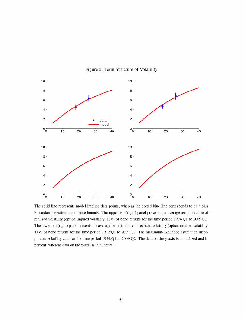
Figure 5: Term Structure of Volatility

0 10 20 30 400

2

4

6

8

10

datamodel

0 10 20 30 400

2

4

6

8

10

0 10 20 30 400

2

4

6

8

10

0 10 20 30 400

2

4

6

8

10

The solid line represents model implied data points, whereas the dotted blue line corresponds to data plus

3 standard deviation confidence bounds. The upper left (right) panel presents the average term structure of

realized volatility (option implied volatility, TIV) of bond returns for the time period 1994:Q1 to 2009:Q2.

The lower left (right) panel presents the average term structure of realized volatility (option implied volatility,

TIV) of bond returns for the time period 1972:Q1 to 2009:Q2. The maximum-likelihood estimation incor-

porates volatility data for the time period 1994:Q1 to 2009:Q2. The data on the y-axis is annualized and in

percent, whereas data on the x-axis is in quarters.

53

Figure 6: Term Structure of Treasury Interest Rates

5 10 15 20 25 30 35 404

4.5

5

5.5

6

6.5

7

7.5

8

8.5

9

datamodel

This figure jointly plots the annualized average yield curve in the sample (with confidence error bounds) and

the model implied yield curve. The maximum-likelihood estimation incorporates bond yield data for the time

period 1972:Q1 to 2009:Q2 and uses only observable macro variables. The y-axis is in percent and the x-axis

is in quarters.

54

Figure 7: Fundamentals and Mispricing: Bond & Option Markets, 1994:Q1 - 2009:Q2

1995 2000 2005 2010

3

4

5

6

7

8

datamodel

1995 2000 2005 2010

4

6

8

10

1995 2000 2005 20102

4

6

8

1995 2000 2005 2010

4

6

8

10

12

1995 2000 2005 2010

4

6

8

10

12

1995 2000 2005 20102

4

6

8

The solid line represents model implied data points, whereas the dotted blue line corresponds to data.

The left part of the picture (from top to bottom) represent: realized volatility, option implied volatility, and

Treasury zero-coupon yield of a 4.5 year Macaulay duration bond. Analogously, the right part of the picture

(from top to bottom) represent: realized volatility, option implied volatility, and Treasury zero-coupon yield

of a 6.5 year Macaulay duration bond. The maximum-likelihood estimation incorporates volatility data for

the time period 1994:Q1 to 2009:Q2 and Treasury yield data from 1972:Q1 to 2009:Q2. The data in this

picture is annualized and in percent. Yellow bars represent NBER recession dates.

55

Figure 8: Volatility Curves

5 10 15 20 25 30 35 40

2

4

6

8

10

12

Monetary ExperimentationGreat ModerationWhole Sample

5 10 15 20 25 30 35 40

2

4

6

8

10

12

This figure presents the model implied term structure of physical volatility (upper panel) and option implied

volatility (bottom panel) for the three periods: Great Moderation, Monetary Policy Experimentation, and the

whole sample. The model is estimated over the whole sample and sample averages are used to construct

the picture. The maximum-likelihood estimation incorporates volatility data for the time period 1994:Q1 to

2009:Q2 and Treasury yield data from 1972:Q1 to 2009:Q2. The data in this picture is annualized and in

percent, the x-axis is in quarters.

56

Figure 9: Option Volatility vs Monetary Policy Uncertainty, 1972:Q1 - 2009:Q2

1975 1980 1985 1990 1995 2000 2005 20101

2.5

4

5.5

7

8.5

10

11.5

1975 1980 1985 1990 1995 2000 2005 20100.128

0.628

1.128

1.628

2.128

2.628

3.128

3.628

4.128

4.6286.5−yr Option Volatility

UncertMP

This figure plots the model implied volatility on a one month option written on a 6.5-year Macaulay duration

Treasury bond (solid line) and the observable real-time measure of Monetary Policy Uncertainty (dotted line)

together with NBER recession dates. The maximum-likelihood estimation incorporates volatility data for the

time period 1994:Q1 to 2009:Q2. The data in this picture is annualized and in percent. Yellow bars represent

NBER recession dates.

57

Figure 10: Impulse Response: Monetary Policy Uncertainty

0 100 200 300 4000

2

4

6

RVol(6.5−yr)

0 100 200 300 4000

2

4

6

TIV(6.5−yr)

0 100 200 300 4000

2

4

6

RVol(4.5−yr)

0 100 200 300 4000

2

4

6

TIV(4.5−yr)

0 100 200 300 4000

0.05

0.1

0.15

0.2 YC slope

This figure presents impulse responses. The driver of monetary policy uncertainty, ηMP is shocked by one

standard deviation and the response on various financial variables is analyzed. The financial variables of

interest are (from top left to bottom right): physical volatility of a 6.5-year Macaulay duration bond, option

implied volatility of a 6.5-year Macaulay duration bond, physical volatility of a 4.5-year Macaulay duration

bond, option implied volatility of a 4.5-year Macaulay duration bond, slope the the Treasury yield curve. The

x-axis is in quarters, numerical values on the y-axis are in percent and annualized. The maximum-likelihood

estimation incorporates volatility data for the time period 1994:Q1 to 2009:Q2 and Treasury yield data from

1972:Q1 to 2009:Q2.

58