economic performances of u.s. non-profit hospitals using ...aabri.com/manuscripts/11869.pdf ·...

Journal of Management and Marketing Research

Economic performances,

Economic performances of U.S. non-profit hospitals using the

Malmquist productivity change index

Chul-Young Roh City University of New York/Lehman College

Changsuh Park

Soongsil University

M. Jae Moon Yonsei University

Abstract

This study evaluated the productivity of non-profit hospitals in the USA in applying DEA-base Malmquist productivity Change index, decomposed into technical efficiency change index and technical progressive change index. Data used for this analysis consisted of 118 non-profit hospital utilization data and financial statements from 1993 through 2003. DEA-based Malmquist was conducted to measure the productivity of non-profit hospitals. This study finds the productivity of non-profit hospitals has increased over the period of 1999-2003. Assessing productivity by hospital size, small-sized hospitals having less than 130 beds are most productive due to technical progress. This study suggests that non-profit hospitals need to downsize their facilities or make adjustments, such as changes of cost structure and facility operation, or adoption of new management to increase productivity. Government bodies also need to develop and enact health policies to ensure that hospitals can increase productivity in both technical progress and efficiency improvement.

Keywords: Hospital Performance, DEA-Malmquist, Non-Profit Hospitals



I. Introduction

Hospital competition and managed care have affected the hospital industry in various

ways. The U.S. hospital industry has become increasingly subject to tighter budget constraints with the implementation of Medicare prospective payment system (PPS) and the growth of managed care. In the current health care environment, competition among hospitals dominates the pricing practice in the hospital industry and has negatively affected hospital costs. Measuring hospital productivity has become an important topic, and it is important to properly measure hospital productivity in order to evaluate the impact of policies on the hospital industry (Walker & Dunn 2006).

Hospital CEOs and administrators, creditors and bondholders, health care consultants, public finance and public accounting researchers, public policy analysts, and the government alike should take interest in this issue of hospitals’ economic performance (Walker & Dunn 2006). For instance, the hospital CEO and administrators should devote themselves to the factors that influence hospitals’ productivity. Public policymakers should pursue possible alternatives to public policy decisions concerning hospital productivity.

Increasing emphasis has been placed on the measures of productivity in hospitals to compare their relative performance given the need to ensure the best use of scarce resources. This paper focuses on a national sample of only non-profit hospitals, mainly due to the availability of data, for the purpose of estimating the productivity of hospitals. However, this weakness of our study in using a sample of non-profit hospitals may not be a significant problem because this is the most common type of hospital in the United States. Although, for-profit and government hospitals play a substantial role in health care delivery in the United States, 61.4% (3,025 hospitals) of the 4,927 hospitals in the United States are classified as non-profit hospitals.1 In addition, this paper is the first study to measure the productivity of non-profit hospitals in the United States.

The primary purpose of this paper is to investigate the economic performance of a national sample of non-profit hospitals, the most prevalent health care service providers in the United States, for the period of 1999-2003. This paper employs Data Envelopment Analysis (DEA) to analyze the productivity of non-profit hospitals in the United States. DEA estimates Malmquist productivity change index, which is a flexible, mathematical programming approach for the assessment of productivity. This study is comprised of 5 parts: literature review; model specification including the specification of factors accounting for hospitals’ economic performance; data and variables used; findings; and, lastly, conclusions.

II. Literature Review

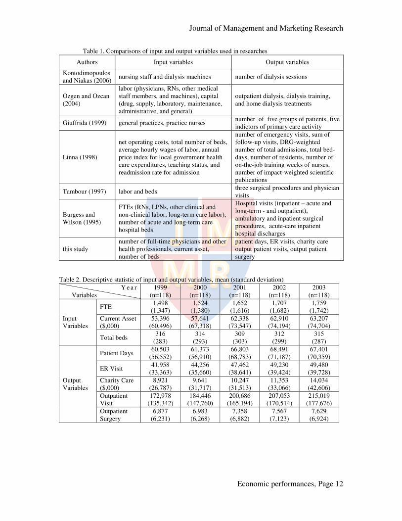
Table 1 compares previous studies’ methods of analysis for assessing hospital productivity by outlining input and output variables. Some studies (Giuffrida, 1999; Linna, 1998; Ozgen & Ozcan, 2004; Tambour, 1997) used panel data to analyze hospital efficiency in detail using a DEA-based Malmquist index. Even though studies using panel data are attractive, the DEA-based Malmquist index is still rarely applied to analysis of health care applications as indicated in Table 1 (Appendix).

1 See AHA 2004, Hospital Statistics (p.6)



In their 1995 study, Burgess and Wilson assess productivity changes between the

years of 1985 and 1988 for a sample of U.S. hospitals that included non-profit hospitals. This analysis focused on estimating technical efficiency by comparing infrastructure and outcome variables. Infrastructure variables consisted of the number of acute-care and long-term hospital beds and the number of full-time equivalents represented by registered nurses, licensed practical nurses, and other clinical and non-clinical staff. Outcomes were measured by the number of acute care and long-term care inpatient days, the number of acute care and long-term care inpatient discharges, the number of outpatient visits, and the number of ambulatory and inpatient surgical visits. The results of this analysis indicated that while non-profit hospitals, along with VA-based hospitals, state and local government hospitals, and for-profit hospitals, experienced intermittent increases in efficiency, decreased technological change counteracted overall productivity.

Linna (1998) measured hospital cost efficiency and productivity in Finland during 1988-1994 using parametric panel models, various DEA models, and the Malmquist productivity index. As output values, he included the total number of emergency visits, the total sum of follow-up visits, the DRG-weighted number of total admissions, the total bed-days, the number of residents, the total number of on-the-job training weeks of nurses, and the total number of impact-weighted scientific publications. He used net operating costs, total number of beds, average hourly wages of labor, annual price index for local government health care expenditures, teaching status, and readmission rate for admission as input variables. He concluded that cost efficiency and technical changes contributed to increase productivity by a 3-5% annual average. Kontodimopoulos and Niakas (2006) estimated the productivity of 73 dialysis establishments in Greece during a 12 year period (1993-2004). They employed a DEA-based Malmquist method that included nursing staff and dialysis machines as input variables and the number of dialysis sessions as the output variables. Though the authors failed to provide a generalized conclusion because of crooked trends, they calculated the productivity indices to progress or regress up to 5% yearly, and they discovered that the technical efficiency change differed from the technical change by 30 %.

Ozgen and Ozcan (2004) analyzed the productivity of 140 free-standing dialysis facilities during the period of 1994-2000 in the USA. They also applied a DEA-based Malmquist index to measure the productivity. They included various output variables (outpatient dialysis, dialysis training, and home dialysis treatments), labor input variables (physicians, RNs, other medical staff members, and machines), and capital input variables (drug, supply, laboratory, maintenance, administrative, and general). They found out that freestanding dialysis facilities did not improve in productivity, but did improve in technical efficiency.

Giuffrida (1999) examined the productivity of primary care service in England from 1991 to 1995 using a DEA-based Malmquist method. He adopted 2 input variables and 10 output variables. He discovered that improvements in technical and scale efficiency contributed to small improvements in total productivity. Technological changes did not significantly affect productivity.

Tambour (1997) used 2 input variables (labor and beds) and 4 output variables (three surgical procedures and physician visits) to estimate the growth in productivity of a



surgical specialty covered by the maximum waiting time guarantee in Sweden. He used a DEA-based Malmquist method, and he focused on the time period from 1988 to 1993. He concluded that positive changes in productivity were mainly due to positive changes in production technology rather than an overall positive change in relative efficiency or scale efficiency. Interestingly, none of DEA-based Malmquist method studies has evaluated the productivity of non-profit hospitals on a national basis. This study uses the first inquiry that measures the productivity of US non-profit hospitals in DEA-based Malmquist method.

II. Model Specification

There are several methods of measuring productivity at the aggregate level or at industrial level. Before the mid-1990s, most studies estimated the total factor

productivity (TFP) by growth accounting method2, or Törnquist productivity index.

Despite the considerable amount of literature, there is no consensus regarding the adequate magnitude of TFP growth rates in the process of economic growth. In addition to the assumptions of perfect competition and constant returns to scale, the basic problems of the growth accounting method are perfect mobility and divisibility of factors and no distortion due to government regulations. It also assumes that the production activities are always efficient, in other words, that outputs are always produced along the production possibilities frontier. One of the recent methods of estimating productivity growth is the Malmquist productivity change index (MPI) method, which became popular after the mid-1990s. This method, without using general or specific production function form, is based on the DEA to construct a piece-wise linear production frontier for each year in a data set. It does not require cost and revenue shares to aggregate inputs, nor does it use a cost minimization assumption. This study adopts the MPI method1 to measure TFP because the MPI method does not need heavy data requirement on output and input variables.

Let the pair of observed input vector xt at time t and the corresponding observed output vector yt at time t be denoted as at = (xt, yt). Then the output distance function at time t is defined as

Dt(at) = infδ

{δ | yt /δ is in Pt(xt)} = [ supδ

{δ | δyt is in Pt(xt)}]-1 (1)

where Pt(xt) = {yt | xt can produce yt} is the production set at time t which is convex, closed, bounded, and satisfies strong disposability of xt and yt (Coelli, 1996). The scalar

δ is a fraction, 0 < δ ≤ 1 for all yt ≥ 0, and δ = 1 if yt is in the production set. Then, the MPI at time t when the production set (technology) is Pt(xt) is defined as Mt = Dt(at+1)/ Dt(at), which is the ratio of the maximum proportional changes in the observed output required to make each of the observed outputs efficient in relation to the technology at time t. Here, Dt(at) is applied to the constant-returns-to scale benchmark. Similarly, the MPI at time t+1 when the production set is Pt+1(x) is Mt+1 = Dt+1(at+1)/ Dt+1(at), which refers to the technology at time t+1. To avoid ambiguity in choosing the production set, the output-oriented MPI is then defined as the geometric mean of the MPI in two consecutive periods (Coelli, 1996; Färe et al., 1994):

2 Growth accounting method is also called Solow’s residual method.



MPIt = (Mt • Mt+1)1/2 =

1/ 21 1 1

1

( ) ( )

( ) ( )

t t t t

t t t t

D a D a

D a D a

+ + +

+

(2)

where MPI > = < 1 implies productivity growth (or change) is positive, zero, or negative from time t to time t+1. Generally, definition (2) may be decomposed into three parts,

MPIt =

1/2t 1 t 1 t t 1 t t

t t t 1 t 1 t 1 t

D ( ) D ( ) D ( )

D ( ) D ( ) D ( )

a a a

a a a

+ + +

+ + +

(3)

EI TI

=

1/2t 1 t 1 t t t+1 t 1 t t 1 t t

t t t t t 1 t 1 t 1 t 1 t 1 t

( ) ( ) ( ) D ( ) D ( )/

( ) D ( ) D ( ) D ( ) D ( )

V a V a V a a a

V a a a a a

+ + + +

+ + + + +

(4)

PI SI TI

The first term in equation (3) is called the efficiency change index (or simply

efficiency index, EI, hereafter), and the second term is the technology change index (or simply technology index, TI, hereafter). Note that the concept of the distance function can be applied to either a constant- returns-to-scale (CRS) or a variable-returns-to-scale (VRS) benchmark. In equation (4), Vt (at) is the output distance function based on a variable-returns-to-scale benchmark. The ratio of Vt+1 (at+1)/Vt (at) is the pure efficiency change index (or simply pure efficiency index, PI, hereafter) from time t to t+1, based on the variable-returns-to-scale technology. The ratio, Vt (at)/ Dt (at), is the scale efficiency index at time t, which measures the output difference between the variable-returns-to-scale technology and the constant-returns-to-scale technology at time t. The ratio of this difference at t and t+1 is the scale efficiency change index from time t to t+1, and is called the scale efficiency change index (or simply scale index, SI, hereafter).

The MPI in equation (2) is the standard definition. It is enigmatic and obscure. Figure 1 indicates a simple diagram to illustrate the basic concepts intuitively. To avoid the cluttering of superscripts, we denote the observed outputs for periods t and t+1 as y

and z, respectively, and the corresponding efficient outputs at time t as y' and z' along the

constant-returns-to-scale technology C', and those at time t+1 as y" and z" along the

constant-returns-to-scale technology C", respectively. Similarly, we denote the efficient

outputs at time t as a' and b' along the variable-returns-to-scale technology C', and those

at time t+1 as a" and b" along the variable-returns-to-scale technology C", respectively

as indicated in Figure 1 (Appendix).

Since, from Figure 1, the definition of the distance function gives Dt (at) = y/y',

etc., the definition of the MPI above reduces to equations (5) and (6) below:

MPI =

1/ 2' "

' "

z y y

y z z



=

1/ 2

/ " " "

/ ' ' '

z z y z

y y y z

= EI× TI (5)

=

1/ 2

/ " '/ ' " "

/ ' "/ " ' '

z b y a y z

y a z b y z

= PI× SI× TI (6)

Thus, the efficiency index EI in (5) is based on the constant-returns-to-scale benchmark, and the pure efficiency index PI in (6) is based on the variable-returns-to-scale benchmark. Both measure the ratio of the degree of deficiencies of the observed

points y to a' for (6) in Figure 1 (or y to y' for (5)) and z to b" for (6) (or z to z" for (5))

relative to the corresponding maximum possible output (a' and b" for (6)) and (y' and z"

for (5)) using the benchmark technology at each period. They reflect the results of learning, knowledge diffusion, spillover across the industrial sectors, improvements in market competitiveness, cost structure, capacity utilization, etc. The scale index SI measures the ratios of the maximum output based on the constant-returns-to-scale technology as compared with the variable-returns-to-scale technology between the two periods. Roughly speaking, Figure 1 measures the change of

the line segment a'y' in the first year to the segment b"z" in the second year. It indicates the change in efficiency due to the scale of production between the two periods. The term in the square root measures the relative movement of the productivity curves based on the constant-returns-to-scale benchmark between two periods and is the

technology index TI, shown by the (geometric) average of the line segment y'y" and z'z" in Figure 1. It represents new product and process innovations, new management systems, or the external shocks that shift the production possibilities frontier.

In this paper, we will refer to the output-oriented MPI simply as the productivity index. When the observed outputs are on the production possibilities curve at each

period, that is, y = y' and z = z", then EI = 1 and, as in Färe et al., (1994), we have TI =

z/y, which is the same as the conventional definition of the TFP ratio between two periods.

IV. Data Source and Variables Used

The data used consisted of hospital utilization data and financial statements, such

as income statements, cash flow, and balance sheets from Merritt Research Services, LLC. To analyze a longitudinal productivity across non-profit hospitals, a final sample of 118 of 3,218 hospitals were identified from 1999 through 2003 (T=5) after all the variables that this study used were cleaned.

Like Lynch and Ozcan (1994), the DEA-based Malmquist method allows flexibility in selecting input and output variables, and results of productivity scores proved to be consistent across various input and output variables. In this paper, 3 input variables are included to measure the resources used in production of non-profit hospitals. The first input variable is the number of full time equivalent (FTE) for physicians and other health professionals for each hospital as a proxy of labor input factor. This variable is intended to reflect the volume and range of work undertaken by health care



professionals in hospitals. The second input variable is the current assets of each hospital as a proxy of capital input factor (resources that the hospitals either has in cash or can convert to cash within one year). This variable indicates how quickly hospitals can pay off obligations that are due in the near future. The current assets become a diagnostic indicator to test the financial health and stability of hospitals (Finkler, 2005). The current assets are deflated using the Consumer Price Index published by the U.S. Department of Labor, Bureau of Labor Statistics. This index was scaled to 100.0 in 1999. The third input variable is the number of hospital beds in a particular hospital, which indicates the size of the hospital. Hospitals with larger bed size should realize economies of scale more easily than hospitals of smaller bed size.

A total of 5 output variables are included in this study. The first output variable considered is the total number of patient days (the sum of the inpatient days of each hospital). A hospital’s total inpatient days reflect a broad measure of its inpatient workload. The other output variables are the number of Emergency Room (ER) visits, outpatient visit, and outpatient surgery visits of each hospital. These output variables indicate the capacity of a hospital’s ambulatory workload and reflect a substantial portion of the total output. The variables are widely accepted in measuring hospital productivity (Harrison et al., 2004). The last output variable in this study is the total amount of charity care (uncompensated care), which is the amount of free care provided to patients who cannot pay for their health care services. Even though charity care is not collected, it is not included as bad debt expense. The level of charity care reflects a hospital’s core competency in delivering health care. The charity care is also deflated using the CPI by the U.S. Department of Labor, Bureau of Labor Statistics. This index was scaled to 100.0 in 1999.

Table 2 shows the descriptive statistics of input and out variables used to measure technical efficiency of non-profit hospitals during 1999-2003 in order to understand the year-specific outputs and inputs. In the input variables, full time equivalent (FTE) was shown to increase over the years, with a five-year average of 1,628 and with an average increase of 4.13% per year, showing that FTE is a main product among multiple input variables. The average current assets with constant dollars increased from $53,396,000 in 1999 to $63,207,000 in 2003, with an average increase of 4.4%. Since 2001, the average amount of current assets slightly increased compared to the time period before 2000. The average bed size fluctuated over the entire period, with the average number of beds being 313.2 as indicated in Table 2 (Appendix).

This study uses 5 output variables: patient days, ER visits, charity care, outpatient visits, and outpatient surgery visits. With a 5 year average of 64,914, the number of patient days slightly increased during the period, but declined in 2003. The average number of ER visits was 46,477 over the 5 years, but the growth rate of ER visits declined overall. The amount of charity care steadily increased over the period, from $8,921,000 in 1999 to $14,034,000 in 2003. The growth rate of charity care, however, increased from 8.1% to 23.6%. Outpatient visits also steadily increased from 172,978 in 1999 to 215,019 in 2003, but the growth rate of outpatient visits declined from 6.6% to 3.8 % over the period. Lastly, outpatient surgery visits steadily increased from 6,877 in 1999 to 7,629 in 2003, but the growth rate of outpatient surgery visits declined from 1.5% to 0.8% over the period.



V. Findings

1. The empirical results of Malmquist productivity change index

This study analyzed the productivity of 118 non-profit hospitals in the U.S.A. during the time period of 1999-2003. Table 3 shows the average values of the Malmquist productivity change index (MPI) and its components: technical efficiency change index (EI), technical progressive change index (TI), pure efficiency change index (PI), and scale efficiency change index (SI) over the period. Over the period, the MPI indicates that non-profit hospitals improved their productivity by 2.1% annually, the TI by 2.5% annually, and the EI by -0.2% annually. The TI (i.e., adoption of new technology, new health care services, new management systems, etc.) reveals similar trends to the MPI during the period. It indicates that the improvement in productivity was driven primarily by the TI, while the EI (i.e., knowledge diffusion, market competition, and cost structure and facility operation) is negative during the period as indicated in Table 3 (Appendix). In accordance with Färe et al. (1994), the EI can be divided into two components in order to explain the regressive shift in technical efficiency change index in detail: PI and SI. During the period focused on in this study, the PI increases, while SI decreases. Technical changes, namely innovations, led the overall productivity trend of non-profit hospitals in the U.S.A. during the period.

It is worth examining the results in detail to find out the effects of technical efficiency of productivity by certain subgroups, such as hospital size and location. Hospitals can be stratified by bed size. This study classifies non-profit hospitals into 3 groups: small-sized, medium-sized and large-sized hospitals. Out of the sample of 118 non-profit hospitals, non-profit hospitals under 130 beds are classified as small-sized (36), hospitals between 131 and 250 beds are classified as medium-sized (39), and hospitals with over 250 beds are classified as large-sized (43).

Table 4 indicates that the geometric mean of the MPI is 1.041 in small-sized hospitals, 1.012 in medium-sized hospitals, and 1.021 in large-sized hospitals, respectively during the period of 1999-2003. Small-sized non-profit hospitals revealed the highest productivity growth, while medium-sized non-profit hospitals increased least productivity growth. The increase of productivity was achieved through TI rather than EI. On the contrary, EI was decreased during the same period. EI decomposes into PI and SI. SI and EI logically demonstrated the same trend as indicated in Table 4 (Appendix).

Hospitals are also characterized by their locations. This study classified hospitals into two location types: urban and rural hospitals3. Out of the 118 non-profit hospitals studied, 66 were located in rural counties, while 52 were in urban ones. According to the results of table 5, during the period of 1999-2003, the productivity growth of urban hospitals is higher than that of rural hospitals. On average, The MPI of urban non-profit

3 The most commonly used and simplistic definitions of rural and urban communities are given by the Office of Management and Budget (OMB) and the Bureau of Census. The OMB makes a dichotomous separation of the country into either Metropolitan Statistical Areas (MSAs) or non-Metropolitan areas, with a metropolitan area defined as either a county with a city of at least 50,000 residents, or urbanized area being part of a county or counties with a minimum of 100,000 inhabitants. The Bureau of Census define an urban area as an any area with a central city with population of 50,000 or more and adjacent territory of more than 2,500 people living outside the central city limits. This study adopts the definition of the Bureau of Census.



hospitals increased in 4 consecutive periods: 1999-2000, 2000-2001, 2001-2002, and 2002-2003 as indicated in Table 5 (Appendix).

However, the MPI of rural non-profit hospitals decreased overall (from 1.024 in 1999 to 1.014 in 2003) as well as in each period with the exception of 2002-2003. TI is the leading source of positive productivity growth in urban non-profit hospitals during the entire period as well as rural non-profit ones in every period except 2002-2003. EI in urban hospitals remains 1.000 on average during the sample period, while EI in rural hospitals showed a negative growth rate of 0.07% on average during the same period. Thus, this result indicates that urban hospitals are more efficient than rural hospitals.

Overall PI of urban hospitals is higher than that of rural hospitals during the period. In detail, the growth rates of PI in urban non-profit hospitals were positive, that is, greater than 1, in 2000-2001 and 2001-2002, while the growth rates of PI in rural hospitals were positive in 2000-2001 and 2002-2003. The empirical results indicate that SI did not exist in rural and urban non-profit hospitals during the period except in 1999-2000.

2. The identification of innovative hospitals

Lastly, this paper investigates which hospitals in the sample make the category-wise best-practice production frontier to shift in each year. We follow Färe, et al. (1994) to identify the “innovators,” which exhibit the following properties:

{TI > 1, Dt(at+1) > 1, Dt+1(at+1) = 1} (7) That is, equation (7) identifies the hospitals that have technology growth at time t, located beyond the previous technology set, but inside the current technology set based on the constant-returns-to- scale technology.

Table 6 shows the number of innovative hospitals by bed size. According to Table 6, the number of innovative hospitals is slightly larger in small sized hospitals in each year over the periods. However, there are no significant differences between medium and large sized hospitals as indicated in Table 6 (Appendix).

In order to analyze the characteristic between innovative and non-innovative hospitals in achieving productivity, the sample is separated into innovative hospitals and non-innovative ones. Figures 2 and 3 show the relationship between EI and TI growth rates for innovative and non-innovative hospitals. The growth rates of EI of innovative hospitals mostly are equal to zero and the growth rates of TI are greater than zero, which implies that there are technical progresses without the improvement of efficiency. On the other hand, in case of non-innovative hospitals, there is a weak negative relationship between the growth rates of EI and TI. Thus, hospitals with technical progress will have a negative growth rate of EI, or vice versa as indicated in Figures 2 and 3 (Appendix).-

Figures 4 and 5 indicate the sources of MPI growth rates, EI or TI, between innovative and non-innovative hospitals. In case of innovative hospitals, the source of MPI growth is TI growth rather than EI growth. In case of non-innovative hospitals, however, EI growth has a positive relationship with MPI growth, but there is a very weak positive relationship between MPI and TI growth rates as indicated in Figures 4 and 5 (Appendix).



In summary, technical progress has an important role in MPI growth in innovative hospitals, while efficiency improvement rather than technical progress has a positive role in MPI growth in non-innovative hospitals.

VI. Conclusion and Policy Implication

The factors that affect the productivity of hospitals have important implications

for stakeholders, such as hospital CEOs and administrators, creditors, bondholders, health care consultants, public policy makers, and governments. Measuring the productivity of hospitals will continue to provoke interest in the current dynamic health care management environment. In this study, technical progressive change index and technical efficiency change index, including pure efficiency change index and scale efficiency change index, for a sample of non-profit hospitals in the USA were estimated. The study used Malmquist productivity change indices, which are linear programming techniques, to measure the growth of productivity. The MPI method is appropriate for this study because it allows multiple input and output variables for non-profit hospitals.

The most critical finding in this study was that the productivity of non-profit hospitals in the USA improved over the 1999-2003 period, especially due to technical progress rather than efficiency improvement. That is, it is concluded that the positive changes in productivity of non-profit hospitals were primarily due to positive changes in technical progress rather than an overall technical efficiency improvement. Facility and market characteristics such as the hospital bed size and location may offer an explanation for policy implications in detail. The results indicate small non-profit hospitals to be most productive due to technical progress. Non-profit hospitals need to downsize their facilities or to make trials, such as changes of cost structure and facility operation or the adoption of new marketing strategies, to increase productivity. Also, the government is a key stakeholder in hospital management, especially for non-profit hospitals in the USA. The government should develop and enact health policies to ensure that hospitals improve productivity, especially technical efficiency.

This study is the first study in measuring the productivity of non-profit hospitals in the USA. The elements of productivity, namely technical progress and technical efficiency, including pure efficiency and scale efficiency, were estimated for each 2 consecutive years over 5 years. Although some interesting facts were observed, it is questionable to generalize the results of this paper for other sectors and for different study periods. Panel study is useful for investigating the trends in measuring productivity over periods. Longitudinal studies should provide insightful information about the effects of health care environments, such as political and economic factors, on productivity. Future productivity research should add measures of health care quality in addition to evaluating productivity of health care organizations. References

American Hospital Association (AHA). (2004). Hospital Statistics, 2004 edition, Chicago, IL: American Hospital Association.



Burgess, J.F. & Wilson, P.W. (1995). Decomposing hospital productivity changes, 1985-1988: A non-parametric Malmquist approach. The Journal of Productivity Analysis, 6, 343-363.

Coelli, T. (1996). A Guide to DEAP Version 2.1: A Data Envelopment Analysis (Computer) Program. CEPA Working Paper 96/08, University of New England, Australia.

Färe, R., Grosskopf, S., Norris, S., & Zang, Z. (1994) Production growth, technical progress, and efficiency change in industrialized countries. American Economic

Review, 84, 66-83. Finkler. S. (2005). Financial Management for Public, Health, and Not-for-Profit

Organizations, 2nd

edition. Upper SaddleRiver, NJ: Pearson Education Inc. Gjuffrida, A. (1999) Productivity and efficiency changes in primary care: A Malmquist

index approach. Health Care Management Science, 2, 11-26. Harrision, J., Coppola, M., & Wakefield, M. (2004). Efficiency of federal hospitals in the

United States. Journal of Medical System, 28(5), 411-422. Kontodimopoulos, N. Niakas, D. (2006). A 12-year analysis of Malmquist total factor

productivity in dialysis facilities. Journal of Medical System, 30, 333-342. Linna, M. (1998). Measuring hospital cost efficiency with panel data models.

Econometrics and Economics, 7, 415-427. Lyunch, J. & Ozcan, Y. (1994). Hospital closure: An efficiency analysis. Hospital and

Health Service Administration, 39 (2), 205-220. Ozgen, H. &, Ozcan, Y. (2004). Longitudinal analysis of efficiency in multiple output

dialyses.” Health Care Management Sciences, 7, 253-261. Tanbour, M. (1997) The impact of health care policy initiatives on productivity. Health

Economics, 6, 57-70. Walker, K.B. & Dunn, L.M. (2006) Improving hospital performance and productivity

with the balanced scorecard. Academy of Health Care Management Journal, 2, 85- 110, 2006.



Table 1. Comparisons of input and output variables used in researches

Authors Input variables Output variables

Kontodimopoulos and Niakas (2006)

nursing staff and dialysis machines number of dialysis sessions

Ozgen and Ozcan (2004)

labor (physicians, RNs, other medical staff members, and machines), capital (drug, supply, laboratory, maintenance, administrative, and general)

outpatient dialysis, dialysis training, and home dialysis treatments

Giuffrida (1999) general practices, practice nurses number of five groups of patients, five indictors of primary care activity

Linna (1998)

net operating costs, total number of beds, average hourly wages of labor, annual price index for local government health care expenditures, teaching status, and readmission rate for admission

number of emergency visits, sum of follow-up visits, DRG-weighted number of total admissions, total bed-days, number of residents, number of on-the-job training weeks of nurses, number of impact-weighted scientific publications

Tambour (1997) labor and beds three surgical procedures and physician visits

Burgess and Wilson (1995)

FTEs (RNs, LPNs, other clinical and non-clinical labor, long-term care labor), number of acute and long-term care hospital beds

Hospital visits (inpatient – acute and long-term - and outpatient), ambulatory and inpatient surgical procedures, acute-care inpatient hospital discharges

this study number of full-time physicians and other health professionals, current asset, number of beds

patient days, ER visits, charity care output patient visits, output patient surgery

Table 2. Descriptive statistic of input and output variables, mean (standard deviation)

Y e a r Variables

1999 (n=118)

2000 (n=118)

2001 (n=118)

2002 (n=118)

2003 (n=118)

Input Variables

FTE 1,498

(1,347) 1,524

(1,380) 1,652

(1,616) 1,707

(1,682) 1,759

(1,742)

Current Asset ($,000)

53,396 (60,496)

57,641 (67,318)

62,338 (73,547)

62,910 (74,194)

63,207 (74,704)

Total beds 316

(283) 314

(293) 309

(303) 312

(299) 315

(287)

Output Variables

Patient Days 60,503

(56,552) 61,373

(56,910) 66,803

(68,783) 68,491

(71,187) 67,401

(70,359)

ER Visit 41,958

(33,363) 44,256

(35,660) 47,462

(38,641) 49,230

(39,424) 49,480

(39,728)

Charity Care ($,000)

8,921 (26,787)

9,641 (31,717)

10,247 (31,513)

11,353 (33,066)

14,034 (42,606)

Outpatient Visit

172,978 (135,342)

184,446 (147,760)

200,686 (165,194)

207,053 (170,514)

215,019 (177,676)

Outpatient Surgery

6,877 (6,231)

6,983 (6,268)

7,358 (6,882)

7,567 (7,123)

7,629 (6,924)



Table 3. Malmquist productivity change index and its components

Period MPI Component

1999-2000

2000-2001

2001-2002

2002-2003

1999-2003

E1 0.989 1.014 0.990 0.997 0.998

T1 1.029 1.013 1.028 1.029 1.025

PI 0.977 1.021 0.999 1.008 1.001

SI 1.014 0.991 0.991 0.989 0.996

MPI 1.018 1.025 1.017 1.025 1.021

Table 4: Malmquist productivity change index and its components by hospital size

Period

MPI Component

1999-2000

2000-2001 2001-2002 2002-2003 1999-2003

EI

Small (n=36) 0.984 1.009 0.991 1.009 0.998

Medium (n=39) 0.988 0.961 1.026 1.000 0.993

Large (n=43) 0.990 1.033 0.978 0.994 0.999

TI

Small 1.079 1.014 1.047 1.032 1.043

Medium 1.032 1.036 1.001 1.009 1.019

Large 1.021 1.005 1.035 1.035 1.024

PI

Small 0.995 1.006 0.993 1.004 0.999

Medium 0.983 0.980 1.018 1.010 0.998

Large 0.972 1.036 0.994 1.007 1.002

SI

Small 0.990 1.003 0.999 1.006 0.999

Medium 1.004 0.980 1.007 0.991 0.995

Large 1.021 0.994 0.984 0.987 0.996

MPI

Small 1.062 1.022 1.037 1.041 1.041

Medium 1.018 0.995 1.025 1.008 1.012

Large 1.011 1.035 1.011 1.028 1.021



Table 5. Malmquist productivity change index and its components by region

Period

MPI Component

1999-2001 2000-2001 2001-2002 2002-2003 1999-2003

EI Rural (n=66) 0.996 0.998 0.960 1.018 0.993

Urban (n=52) 0.985 1.024 1.007 0.985 1.000

TI Rural 1.028 1.026 1.036 0.997 1.022

Urban 1.029 1.005 1.024 1.048 1.027

PI Rural 0.987 1.005 0.971 1.022 .0996

Urban 0.971 1.029 1.016 0.999 1.004

SI Rural 1.010 0.992 0.989 0.996 0.997

Urban 1.016 0.991 0.992 0.985 0.996

MPI Rural 1.024 1.022 0.993 1.014 1.013

Urban 1.014 1.026 1.030 1.031 1.025

Table 6. Distributions of innovative hospitals by bed size

Year Bed size

2000 2001 2002 2003 Total

1300 ≤≤ beds 6 8 8 7 29

250131 ≤≤ beds 5 4 5 4 18

251≥beds 5 3 5 4 17

Total 16 15 18 15 64



Figure 1. Output distance function

Figure 2. EI and TI growth rates of Figure 3. EI and TI growth rates of

innovative hospitals non-innovative hospitals

-0.4-0.20.00.20.40.6-0.4 -0.2 0.0 0.2 0.4 0.6 0.8EI growth rateTI growth rate TIgr = -0.200EIgr + 0.015R2 = 0.109

-0.4-0.20.00.20.40.6-0.4 -0.2 0.0 0.2 0.4 0.6 0.8EI growth rateTI growth rate

0Input

Output

y

z

b'

z"

b" y"

a"

y'

a'

z'

V'

V"

C'

C"



Figure 4-1. EI and MPI growth rates of Figure 4-2. TI and MPI growth rates of innovative hospitals innovative hospitals

-0.4-0.20.00.20.40.60.8-0.4 -0.2 0.0 0.2 0.4 0.6 0.8EI growth rateMPI growth rate -0.4-0.20.00.20.40.60.8

-0.4 -0.2 0.0 0.2 0.4 0.6 0.8TI growth rateMPI growth rate

Figure 5-1. EI and MPI growth rates of Figure 5-2. TI and MPI growth rates of

non-innovative hospitals non-innovative hospitals MPI = 0.817EI + 0.014R2 = 0.677-0.4-0.20.00.20.40.60.8

-0.4 -0.2 0.0 0.2 0.4 0.6 0.8EI growth rateMPI growth rate MPI = 0.432TI - 0.001R2 = 0.069-0.4-0.20.00.20.40.60.8

-0.4 -0.2 0.0 0.2 0.4 0.6 0.8TI growth rateMPI growth rate

economic performances of u.s. non-profit hospitals using ...aabri.com/manuscripts/11869.pdf ·...

Documents