economic outlook 20162016 1 u.s. economy continues to show moderate growth the current macroeconomic...

Economic Outlook2016University of Nevada, Las Vegas

SPONSORING HOST

CHAIRMAN’S CIRCLE

DIAMOND CIRCLE

PRESIDENTIAL CIRCLE

EXECUTIVE CIRCLE

Growing to better serve theLas Vegas community with

all of their real estate needs.

Frank Nason • 702-595-2800Tamra Coulter • 702-460-8835

Serving the Las Vegas, Reno-Sparks and the Mountain Southwest since 1994, Residential Resources has been providing in-depth residential and commercial real estate market analysis and recommendations. We provide that same level of market intelligence and statistical analysis to our individual buyer and seller clients providing an edge few other Realtors or real estate companies can o�er. We’re a company where listening and integrity come �rst. Proud members of both the Greater Las Vegas and Reno-Sparks Associations of Realtors.

702-597-2855 • ResidentialResources.com

Nevada Broker License B.0033121

The Lee Business School leverages the research and service mission of the Center for Business and Economic Research to create mutually beneficial relationships with the business community. Through our partnerships we create valuable opportunities for faculty to engage in projects that transform the lives of our students and the communities we serve.

Please join us in thanking the following organizations for five years of continuous support to the Center for Business and Economic Research.

To learn more about CBER, visit us at cber.unlv.edu

THANK YOU

SUCCESSFUL LEADERS BUILD STRONG PARTNERSHIPS

Growing to better serve theLas Vegas community with

all of their real estate needs.

Frank Nason • 702-595-2800Tamra Coulter • 702-460-8835

Serving the Las Vegas, Reno-Sparks and the Mountain Southwest since 1994, Residential Resources has been providing in-depth residential and commercial real estate market analysis and recommendations. We provide that same level of market intelligence and statistical analysis to our individual buyer and seller clients providing an edge few other Realtors or real estate companies can o�er. We’re a company where listening and integrity come �rst. Proud members of both the Greater Las Vegas and Reno-Sparks Associations of Realtors.

702-597-2855 • ResidentialResources.com

Nevada Broker License B.0033121

Colliers International has more than 20 years of commercial real estate history in Las Vegas. For a decade running, Colliers Las Vegas has been chosen by its peers and named Brokerage Firm of the Year. This longevity in market leadership coupled with the accuracy of our database make Colliers Quarterly Reports your go to stop for a timely and reliable economic outlook. This is what we do. We are number one for a reason – let us show you the way.

Download Quarterly Reports Today on the Following Disciplines:

• Industrial• Office• Retail• Medical Office• Land• Hotel• Multi-Family

colliers.com/lasvegas/insights

QUARTERLY REPORTSResearch

LAS VEGAS

MARKETLEADER“A leader is one who knows the way, goes the way and shows the way.”

- John C. Maxwell

NEVADA SYSTEM OF HIGHER EDUCATION

BOARD OF REGENTSCHAIRMAN Rick Trachok

VICE-CHAIRMAN Michael B. Wixom REGENT Andrea Anderson, PhD

REGENT Cedric CrearREGENT Robert M. Davidson

REGENT Mark W. Doubrava, MDREGENT Jason Geddes, PhD

REGENT Trevor Hayes REGENT James Dean Leavitt

REGENT Sam LiebermanREGENT Kevin C. Melcher

REGENT Kevin J. Page REGENT Allison Stephens

CHIEF OF STAFF AND SPECIAL COUNSEL TO THE BOARD Dean J. Gould

UNIVERSITY OF NEVADA, LAS VEGASPRESIDENT Len Jessup, PhD

LEE BUSINESS SCHOOLDEAN Brent Hathaway, PhD

CENTER FOR BUSINESS & ECONOMIC RESEARCH

DIRECTOR & PROFESSOR OF ECONOMICS Stephen M. Miller, PhDASSOCIATE DIRECTOR & ASSOCIATE PROFESSOR OF ECONOMICS Constant Tra, PhD

ASSOCIATE DIRECTOR OF RESEARCH & ADMINISTRATION, DIRECTOR OF SURVEYS, DIRECTOR OF NEVADA KIDS COUNT Rennae Daneshvary, PhD

ECONOMIST Giorgio Canarella, PhDECONOMIC ANALYST Jinju Lee

RESEARCH & GRANTS COORDINATOR Richard BolandRESEARCH ASSOCIATE Peggy Jackman

GRADUATE ASSISTANT Shi Yan LiuGRADUATE ASSISTANT Yan Mikhaylov

GRADUTE STUDENT WEBSITE ADMINISTRATOR Laila Davis

CONFERENCE SPONSORS

DIAMOND CIRCLE M Resort Spa CasinoDIAMOND CIRCLE The Venetian | The Palazzo

CHAIRMAN’S CIRCLE Bank of NevadaPRESIDENTIAL CIRCLE Nevada Hotel & Lodging Association

PRESIDENTIAL CIRCLE Mitsubishi Cement CorporationPRESIDENTIAL CIRCLE WageWatch

EXECUTIVE CIRCLE Silver State Schools Credit UnionEXECUTIVE CIRCLE Velstand Investments, LLCEXECUTIVE CIRCLE Heck Wealth Management

Center for Business & Economic ResearchBox 456002 | 4505 South Maryland Parkway

Las Vegas, Nevada 89154-6002Telephone: (702) 895-3191

email: [email protected]

12016

U.S. Economy Continues to Show Moderate Growth

The current macroeconomic environment confronts policy makers and economic analysts with much difficulty in trying to make sense out of where the economy is headed. For example, the Congressional Budget Office (CBO) calculates the path of potential real gross domestic product (GDP). Since the Great Recession, potential output follows a long-term trend growth rate of around 2 percent, defining a new and lower long-term growth rate for the U.S. economy. While the current recovery confined itself to a slow to moderate growth rate, this path proves consistent with the new normal described by the CBO’s calculation of potential real GDP.

The views expressed are those of the authors and do not necessarily represent those of the University of Nevada, Las Vegas or the Nevada System of Higher Education.

2

Our forecast of real GDP growth of slightly below 2 percent in 2016 and slightly above 2 percent in 2017 (Figure 1) reflects this “new normal” long-term growth rate. The confidence band around our forecast, however, provides substantial room to encompass many of the extant forecasts in the market. Our forecast falls on the pessimistic (lower) side of the consensus. But, the existing consensus moves in our direction with each new forecast release.

Since the Great Recession, the U.S. economy has experienced modest growth as we now enter the seventh year of the recovery.1 The Federal Reserve (Fed), after an extended run of Quantitative Easing (QE), now contemplates raising interest rates in December of this year, although some analysts think that this will not occur until 2016.

The Fed currently faces the task of unwinding its unprecedented holding of assets. During the

1. Note that the average expansion over the post-1980 period equals seven years.

various phases of QE, the Fed’s balance sheet exploded from just under $1 trillion in assets, largely Treasury issues, to around $4.5 trillion in assets with around 40 percent still in mortgage-backed securities (MBS) of unknown quality.

While interest rates remain at historically low levels and the U.S. infrastructure can use significant expenditure to upgrade systems, implementing such a fiscal expansion seems unlikely to occur given the political obstacles to such legislation. One advantage of such infrastructure spending is that it provides a one-off event that disappears from the federal budget once the infrastructure projects are completed and go online.

In the global economy, weakening growth in China and the implied spillover effects on the emerging market economies that rely on commodity exports to China portend weakening global economic activity. The strengthening of the U.S. dollar also will slow U.S. growth, as net exports will worsen as exports fall and imports rise.

Figure 1. Growth Rate of U.S. Real GDP

Sources: U.S. Bureau of Economic Analysis; Center for Business and Economic Research, UNLV

3

Contributions to U.S. Economic Growth During 2014, U.S. real GDP grew by 2.4 percent (Table 1) with wide swings in quarterly growth rates. Consumer spending and business fixed investment contributed the most to this growth, while government spending and net exports subtracted from it.

After spending fell in first quarter of 2014, its bounce back was observed in nearly every spending category for the second and third quarters. Personal consumption increased sharply in the second and third quarters. Inventory accumulation was also strong in the second quarter. More modest increases in residential investment and government purchases occurred. Net exports also showed favorable trends. In the

Table 1. Contributions to the Growth of U.S. Real GDP

Note: Data are reported at seasonally adjusted annual rates.Source: U.S. Bureau of Economic Analysis

fourth quarter, however, only consumer spending remained strong. For the remainder of 2015, we expect much lower growth in real GDP. The components of spending that play an important role, aside from consumption, are net exports and inventory investment (Table 2). We anticipate that final domestic sales will continue to contribute to overall growth at a more than 2.5 percent rate.

Consumer Spending. Consumer spending, the largest component of U.S. real GDP, currently accounts for around 68 percent of total spending. From 1947 through 2014, the annual growth rate in real consumer spending averaged 3.4 percent. It grew at about two-thirds of this average—2.4 and 2.5 percent during 2013 and 2014, respectively. After averaging around 2 percent in 2015, we

Table 2. Forecast Contributions to the Growth of U.S. Real GDP

Note: Data are reported at seasonally adjusted annual rates.Source: Center for Business and Economic Research, UNLV

2013 2014 2015

I II III IV I II III IV I II III

Real GDP (% change annual rate) 1.9 1.1 3.0 3.8 -0.9 4.6 4.3 2.1 0.6 3.9 2.1

Contributions to Real GDP Growth

Final Domestic Sales 1.63 0.99 1.34 2.64 1.76 3.68 3.90 3.00 1.70 3.71 2.89

Personal Consumption 1.74 0.96 1.17 2.36 0.85 2.60 2.34 2.86 1.19 2.42 2.05

Business Fixed Investment 0.51 0.14 0.44 1.05 1.00 0.56 1.12 0.09 0.20 0.53 0.31

Residential Investment 0.26 0.27 0.15 -0.26 -0.09 0.31 0.11 0.31 0.32 0.30 0.24

Government Purchases -0.88 -0.38 -0.42 -0.51 0.00 0.21 0.33 -0.26 -0.01 0.46 0.29

Net Exports -0.01 -0.24 0.16 1.26 -1.39 -0.24 0.39 -0.89 -1.92 0.18 -0.22

Exports 0.12 0.64 0.55 1.42 -0.95 1.28 0.24 0.71 -0.81 0.64 0.11

Imports -0.13 -0.89 -0.39 -0.16 -0.44 -1.52 0.15 -1.60 -1.12 -0.46 -0.33

Inventory Investment 0.28 0.38 1.48 -0.08 -1.29 1.12 -0.01 -0.03 0.87 0.02 -0.59

2015 2016 2017

IV I II III IV I II III IV

Real GDP (% change annual rate) 2.3 1.6 1.6 2.0 1.9 2.1 2.2 2.2 2.3

Contributions to Real GDP Growth

Final Domestic Sales 2.9 2.1 2.3 2.7 2.7 2.3 2.3 2.6 2.7

Personal Consumption 2.1 1.7 1.6 1.8 1.9 1.9 1.6 1.7 1.9

Business Fixed Investment 0.3 0.2 0.3 0.3 0.3 0.2 0.3 0.3 0.3

Residential Investment 0.3 0.4 0.3 0.4 0.3 0.4 0.3 0.4 0.3

Government Purchases 0.2 -0.2 0.1 0.2 0.2 -0.2 0.1 0.2 0.2

Net Exports -0.6 -0.4 -0.5 -0.6 -0.6 -0.3 -0.2 -0.2 -0.2

Inventory Investment 0.0 -0.1 -0.2 -0.1 -0.2 0.1 0.1 -0.2 -0.2

4

investment into the United States and keep net exports in the negative range in 2016 and 2017.

2. Interest Rates and Monetary Policy: “Maximum Employment and 2 Percent Inflation”

At their last meeting, the Federal Open Market Committee (FOMC) decided to hold the line

on the first interest rate increase until later this year at its December meeting, or possibly into 2016. Fed Chairman Yellen still links monetary policy decisions on interest rates to the dual goals of “maximum employment and 2 percent inflation.” That is, the Fed will only begin to raise interest rates when it feels that the labor markets have returned to a normal situation, and that inflation is well on its way to the target of 2 percent. Since the last FOMC meeting, much, but not all, of the economic news for both employment and inflation provides the opponents of an interest rate hike in 2015 with more ammunition. But, most analysts now expect the FOMC to pull the trigger and raise interest rates at its December meeting.

In sum, the outlook for interest rates remains dominated by monetary policy. With the economy operating below potential, the FOMC has held short-term interest rates at extremely low levels (Figure 2). When the Fed begins to raise interest rates, a new question emerges. How fast will interest rates rise?

Because the economy currently operates below its potential, and we are not yet seeing widespread signs of labor market tightness or sustained inflation anywhere close to 2.0 percent, any interest rate hike implemented by the FOMC will likely occur near the end of 2015, or early in 2016. Even with the anticipated tightening, interest rates will probably remain well below historical averages over the next few years. One pundit quipped that the Fed’s tightening will be the “easiest tightening” on record.

The Fed’s policy of QE also has attempted to drive long-term interest rates lower. In 2014, the Fed began tapering its QE, which led many to expect rising long-term interest rates. Weakness elsewhere in the world, as well as the adoption

expect real consumer spending to grow more slowly in 2016 and 2017.

Private Investment. Private investment spending, a more volatile component of U.S. real GDP, currently accounts for about 16.8 percent of total spending. From 1947 through 2014, the annual growth rate of real private investment averaged 4.4 percent. It grew somewhat above this average rate—4.5 and 5.4 percent growth rates in 2013 and 2014, respectively. Within the real private investment category, residential and business fixed investment grew at 5.5 and 6.4 percent annual rates, respectively, in 2014. Business fixed investment tailed off substantially in 2015, while residential investment continued to move at a brisk pace.

After its strong performance in 2014 and mixed performance in 2015, we expect slower gains in business fixed investment in 2016 and 2017. We see residential investment contributing slightly less to overall investment activity in the near term as the housing market experiences a pause in its forward momentum. Inventory investment, which subtracted significantly in the third quarter of 2015, should become a relatively benign contributor to real growth going forward.

Government Spending. Total government spending (federal, state, and local) on goods and services accounts for 18.8 percent of total spending. From 1947 through 2014, the annual growth rate of total real government spending on goods and services was 2.8 percent. This component declined by 2.0 and 0.2 percent in 2013 and 2014, respectively. Even though an improving economy will generate increased tax revenue, we expect the slowed growth in the economy and the current mood of fiscal conservatism to slow the growth of government spending in 2016 and 2017.

Net Exports. Exports provided significant strength in the early stages of the U.S. economic recovery. A strong surge in the last quarter prevented net exports from making a negative contribution in 2013. But, in 2014, a stronger U.S. economy attracted more foreign investment and imports. Lower oil prices helped to reduce imports, but not enough to offset other factors. We expect that weak economic activity elsewhere in the world and the stronger dollar will gradually boost foreign

5

of QE by numerous central banks around the world, generated an influx of foreign investment to the United States, which held down long-term rates, such as those for 10-year Treasury notes and conventional mortgage rates. Nonetheless, the current positive spread of the long-term over the short-term interest rate does not offer any signal about a potential recession.

The U.S. economic recovery continues with many pundits predicting an improving trajectory over the next two years. That is, many expect the real GDP growth rate to experience a significant uptick to above 3 percent. The Fed has been following a policy of tapering its acquisition of new assets, that is, by stopping its QE. But the Fed still must unwind its unprecedented holding of assets—largely U.S. Treasuries and mortgage-backed securities—without either triggering a slump back into recession or igniting a significant spike in inflation.2

After the financial crisis, the Fed drove the federal funds rate below 1 percent in August 2008 and quickly moved the rate to under 0.25 percent or

2. Many analysts credit the Fed with preventing another Great Depression, but a few analysts criticize the Fed’s low interest rate policy prior to the financial crisis that fed, in this view, the housing price bubble. To wit, the federal funds rate fell below 2 percent at the end of 2001, reaching a low of 1.0 percent in early 2004 before rising to 5.25 percent in August 2006.

25 basis points, basically achieving a zero lower-bound interest rate. Having lost traction with its traditional monetary policy tool of lowering the short-term interest rate, the Fed turned to a new tool, QE. During the various QE programs, the Fed grew its balance sheet from about $1 trillion in assets in August 2008 to over $4.5 trillion today, as shown in Figure 3.

The various QE programs also drove the composition of the Fed’s balance sheet from its traditional holding of largely U.S. Treasury issues toward MBS. Figure 4 illustrates the percentage of the Fed’s assets in U.S. Treasuries (black line), MBS (green line), and borrowed reserves (red line) over time. One can note that the holding of U.S. Treasuries as a percentage fell dramatically before the acquisition of MBS began their rise as a percentage. The difference largely reflects a short period of time when banks borrowed enormous amounts of reserves from the Fed. For a number of months during the crisis, the banking system held negative non-borrowed reserves. In other words, the banking system borrowed more reserves from the Fed than the banking system actually held in its reserve accounts.

Figure 2. Interest Rates to Rise

Sources: Board of Governors of the Federal Reserve System; National Bureau of Economic Research; National Bureau of Economic Research; Center for Business and Economic Research, UNLV

6

Figure 4. Treasuries, Mortgage-Backed Securities, and Borrowed Reserves as Percent of Federal Reserve Assets

Figure 3. Size of Federal Reserve’s Balance Sheet (assets)

Sources: Board of Governors of the Federal Reserve System; National Bureau of Economic Research; Center for Business and Economic Research, UNLV


7

At the same time, bank excess reserves exploded from $2 billion to $2.6 trillion (Figure 5). Bankers typically argue that the accumulation of excess reserves occurred because of limited requests for credit—a lack of demand. Small businesses, who successfully qualify for credit, typically argue that they cannot afford the loan terms—a lack of supply. Bankers respond that the regulators required the tightening of credit terms. Currently, the banking system holds $1.72 in reserves against every dollar of transactions (checking) accounts. Such numbers are unprecedented.

Much of the unprecedented holding of reserves by the banking system reflects the noted decision of the Fed to pay interest on bank excess reserves in October 2008. When the 0.25 percent (25 basis points) interest rate exceeds the Fed’s targeted federal funds rate, little incentive exists for banks to loan overnight funds to other banks. Rather, banks just continue to hold their excess liquidity on deposit at the Fed. Moreover, the large supply of excess reserves provides the fuel that could ignite a destructive inflation. That is, according to a few analysts, the return to more normal credit market conditions will see the dramatic increase in credit and money creation, leading to significant

inflation. In other words, the huge supply of excess reserves could quickly turn into lots of money and credit.

The Fed recently published its policy normalization principles and plans. By policy normalization, the Fed means “raising the federal funds rate and other short-term interest rates to more normal levels.” To normalize, the Fed will use the interest rate that it pays on excess reserves. In addition, once the Fed begins the process of normalization, it will also begin winding down its asset holds from the current level of over $4 trillion to a more normal level by not reinvesting principal repayments on assets held by the Fed.

Traditionally, the Fed implements a tightening of monetary policy by selling government securities in the open market. Such action withdraws liquidity, lowers asset prices, and drives up interest rates. But, when the economy recovers, withdrawing liquidity too quickly can drive up interest rates too high, stalling the recovery. Withdrawing the liquidity too slowly can leave interest rates too low, overheating the economy and igniting inflation.

Figure 5. Total Banking System Excess Reserves


8

As noted above, the Fed now plans to maintain the size of its balance sheet after QE ceases until it begins to “normalize” by raising interest rates. When this normalization begins, the Fed will raise the interest rate on excess reserves to lock them up and to prevent the banking system from financing excessive money and credit creation. Only after normalization begins will the Fed begin to reduce the size of its balance sheet and then only by the pace of principle repayments on the assets in its balance sheet.

This new strategy, however, faces the same dangers as the more traditional approach. If the Fed responds too slowly and the interest rate on excess reserves does not rise enough, then more money and credit creation will occur than planned, which can overheat the economy and spark inflation. If the Fed reacts too quickly and drives the interest rate on excess reserves too high, then too little money and credit creation will occur, slowing the economic recovery and possibly triggering a return to recession.

This new strategy also introduces a new danger. When the private sector demands more credit for spending, the excess reserves needed to finance more demand for credit already exists on bank balance sheets. Thus, credit and money growth can occur even without explicit Fed action. The Fed will then react to, rather than lead, events.

No matter which strategy the Fed adopts, the same risks exist. The Fed needs a Goldilocks story—neither too little nor too much credit creation, just the right amount. The Fed currently travels over unmapped terrain and the possibility of making wrong turns is high. The worst-case scenario, however, could occur even absent Fed errors. To wit, so much liquidity may exist in the system that the required increase in the interest rate on excess reserves to prevent too rapid an increase in money and credit may plunge the economy back into recession and absent that increase in interest rates, the growth in money and credit may prove too expansive, leading into an economy with way too much inflation. In other words, the Fed’s past policies may have created a situation where no exit strategy can occur without significant pain, recession, inflation, or possibly both.

Nevertheless, given where we are today, the current strategy of using the interest rate on excess reserves to lock up those reserves in the short run and withdrawing the excess liquidity from the system in a sustained and systematic manner is the best policy choice. This choice also may give the Fed more control over the economy. That is, this strategy may reduce the ability of banks to supply increased demands for credit without explicit Fed action, a problem that inherently exists with all the excess liquidity in the system.

3. Global Economic Activity

In 2014, the world economy showed relatively constant growth, but at lower rates than prior

to the Great Recession. The Chinese economy continues to experience slower growth with the recent volatility of asset prices (stocks and houses), worrying analysts about further reductions in Chinese growth. World economic growth equaled 3.3 and 3.4 percent in 2013 and 2014, respectively (Figure 6). For 2015, the International Monetary Fund (IMF) expects world economic activity to slow to a 3.1 percent rate, with a gradual acceleration thereafter driven by the developing world up to a growth rate of 4.0 percent. Whether such projections of a rising trend in world economic growth materialize depends greatly on the eventual outcomes in the euro zone and China. The slower growth in China exerts spillover effects on those emerging market economies that export commodities to China. That is, the slowing of growth in China means reduced demand for commodities and, thus, slower growth in supplier countries. The advanced country group (the G7) grows the slowest, equaling only 1.8 percent in 2014 and an expected 2.0 percent in 2015. The advanced economies’ growth rate remains relatively constant and ending the forecast horizon at 1.9 percent growth. The Asia Pacific region generally leads the groups of countries in economic growth. The forecast shows them returning to a growth rate in the 6.5 percent level in the last three years of the forecast period. The emerging market group of countries experienced 4.6 percent growth in 2014 and an expected slowing to 4.0 percent growth in 2015. By the end of the forecast horizon, emerging market growth recovers to 5.3 percent.

9

China now plays a bigger role in the world economy as the sheer size of its economy now rivals the U.S. economy. That is, comparing nominal GDPs in China and the United States, using purchasing power parity comparisons, China passed the United States in size in 2014 (Figure 7). In addition, as China grows bigger, it proves more difficult to continue to grow at double-digit rates (Figure 8). We see that the growth rate in China has fallen over the past several years and will probably glide toward growth rates in the developed world in the not too distant future. The U.S. growth rate seems to correspond to a 2-percent level while the Chinese growth rate has fallen to nearly 6 percent. Nonetheless, China still trails the United States in per capita GDP (Figure 9).

Recently, China announced that it will revoke the one-child policy. This policy has created a couple of unintended consequences. First, the marriage market is in disequilibrium as the country has too many eligible men relative to eligible women. Second, the traditional role of children and grandchildren supporting parents and grandparents in their older years will experience a

huge shock as the ratio of older people to working age people will rise dramatically in the coming years.

4. Indicators of Economic Activity and Confidence

Everything is in place for stronger economic growth, but we have yet to see signs

of acceleration. The financial positions of individuals, firms, and the financial sector are all in sufficiently good shape to support the strong spending necessary to drive a strong acceleration in U.S. economic activity.

U.S. Leading Index. The U.S. Leading Economic Index has been fluctuating in the range of 1 to 2 percent (Figure 10), which signals continued economic growth. This indicator does not provide any signal of a recession in the near future.

Figure 6. Global Economic Growth

Source: International Monetary Fund

10

Figure 8. China and the United States Real Growth Rates (national currencies)


Figure 7. Nominal GDP China and the United States - Purchasing Power Parity (PPP) Values


11

Figure 9: Nominal GDP per Capita - PPP Values


Figure 10. U.S. Leading Economic Index

Sources: Philadelphia Federal Reserve Bank; National Bureau of Economic Research; National Bureau of Economic Research

12

investment and accelerating economic activity during upcoming months. The index jumped back above the historical average in August and September 2015, raising some concern about the future path of the economy. Other issues, such as business confidence in the economy and weak Chinese and European economies, continue to pose impediments to robust investment and an accelerating economy.

Consumer Confidence Index. The University of Michigan measure of consumer confidence has followed a bumpy upward path since the Great Recession. It nearly returned to a level of 100 in January 2015, but since then it has tracked on a downward path throughout this year. We inverted the Economic Policy Uncertainty Index and plotted it on the same graph as the consumer confidence index (Figure 13). The consumer confidence index and the inverted economic policy index track each other with a correlation of 0.63. Recently, the uncertainty index experienced decreases since August 2014 and, as noted above, the consumer confidence index has fallen since January 2015.

Term Structure of Interest Rates. A good indicator of recessions is the term structure of interest rates, which examines the differences in interest rates at a point in time for different maturities of U.S. Treasury issues (bills, notes, and bonds). Figure 11a shows the time-series properties of the term structure of nominal interest rates (i.e., not adjusted for inflation), plotting the 3-month and one-year Treasury bills, the 3-, 5-, and 10-year Treasury notes, and the 20- and 30-year Treasury bonds. We note that prior to recessions, the short-term interest rates rise and the spread between the short-term and long-term interest rates disappears, or even reverses itself. This is called an inverted term structure (yield curve), when the short-term interest rate exceeds the long-term interest rate. This typically happens when the inflation rate is high, causing the nominal interest rate to go up. High inflation usually associates with the Fed taking away the “punch bowl” and creating a recession. But the markets do not expect the inflation rate to continue at a high level. Thus, long-term interest rates have a lower inflation premium built into their rate, leading to an inverted term structure. Currently, the long-term interest rates exceed the short-term interest rates, suggesting that a recession is not in the cards.

When we subtract the inflation rate from the nominal interest rate, we produce a real interest rate. That is, for a lender, after setting aside some of the interest rate to cover the inflation rate, the residual amount reflects a real return to the lender. Figure 11b plots the real 3-month and one-year Treasury bills, the real 3-, 5-, and 10-year Treasury notes, and the real 20- and 30-year Treasury bonds. Once again, we see that prior to recessions the real short-term interest rates move upward closing the gap on the real long-term interest rates. Once again, the long-term real interest rates exceed the short-term real interest rates, suggesting that a recession is not around the corner.

Economic Policy Uncertainty. Since the end of the Great Recession, uncertainty about U.S. economic policy has impeded business investment (Figure 12), which has slowed the recovery. Nonetheless, uncertainty about U.S. economic policy fell below its historical average in May 2015, which suggested that policy uncertainty was not much of an impediment to increased

13

Figure 11b. Real Treasury Interest Rates

Sources: Federal Reserve Bank of St. Louis (FRED); National Bureau of Economic Research

Figure 11a. Nominal Treasury Interest Rates

Sources: St. Louis Federal Reserve Bank (FRED); National Bureau of Economic Research

14

Figure 13. Consumer Confidence and U.S. Economic Policy Uncertainty Index (inverted)

Sources: University of Michigan Survey Research Center; Economic Policy Uncertainty <http://www.policyuncertainty.com/; National Bureau of Economic Research

Figure 12. U.S. Economic Policy Uncertainty Index

Sources: Economic Policy Uncertainty <http://www.policyuncertainty.com/>; National Bureau of Economic Research

15

5. Employment Sector Remains Strong

Since CBER constructs the CBER-DETR Coincident Employment Index (see next

section for the Nevada Outlook), we also track the same index at the national level. The U.S. Coincident Employment Index (Figure 14) includes four employment measures—household employment, nonfarm employment, the unemployment rate (inverted, since an upward movement in the jobless rate is a “negative”), and the insured unemployment rate (inverted). Of the six recessions depicted in Figure 14, the Great Recession shows the deepest drop. In addition, the recovery from the Great Recession depicts a V-shaped recovery, unlike the recessions in the early 1990s and 2000s, where the “jobless recovery” phrase described those two recoveries. Finally, the index rose above its precession peak in October 2014, or five years to the month after its trough in October 2009.

With job growth, the U.S. unemployment rate fell sharply from July 2014 through April 2015 (Figure 15). The unemployment rate now holds at 5.0 percent in October. Initial claims for unemployment also followed a downward trend, which means the economy has been doing more to create jobs than destroy them.

Figure 14. U.S. Coincident Employment Index

Sources: U.S. Bureau of Labor Statistics; National Bureau of Economic Research

16

Lower Oil Prices. As the result of fracking, conservation, fuel switching, increased oil production and weakness in the Chinese and European economies, oil prices have fallen by about half since mid-summer 2014 (Figure 16). Over the 2015-2016 time period, the futures market indicates average oil prices of about 55 percent of summer 2014 high prices. If these lower oil prices are sustained, the U.S. economy should see a net stimulus that amounts to a one-time gain of 0.7 to 1.0 percent spread out over the next several years.

Lower oil prices provide U.S. consumers with what amounts to an annual increase in disposable income because they spend less on gasoline. But, the issue is what consumers do with the higher disposable income—increase consumption or increase saving. The permanent income hypothesis tells us that consumers when faced with a temporary increase in disposable income will use most of this increase to increase their saving (reduce their debt). It is only when the increase in income is viewed as permanent that consumers will increase their consumption by significant amounts. The evidence on temporary tax cuts suggests that consumers only spend around 20 percent of the

tax decrease. Researchers found that the fall in energy prices did not generate a big increase in consumption, and that rising consumption still has not occurred to a significant extent.

U.S. Housing Market Remains Tight. As shown in Figure 17, the U.S. housing supply is fairly tight. Based on recent sales, the current houses listed on the market provide only 5.3 months of supply, which is below the historical average of 6.1 months. As long as supply remains below average, prices can be expected to continue rising, and home construction will be stimulated. Nevertheless, we expect housing construction to remain somewhat subdued in the immediate future.

Figure 15. Unemployment and Initial Claims for Unemployment

Sources: U.S. Bureau of Labor Statistics; National Bureau of Economic Research

17

Figure 16. Brent Oil Price

Figure 17. U.S. Housing Market Remains Somewhat Tight

Sources: U.S. Census Bureau; National Bureau of Economic Research

Sources: U.S. Bureau of Labor Statistics; New York Mercantile Exchange; National Bureau of Economic Research; Center for Business and Economic Research, UNLV

18

latter the result of reduced business investment. These developments have led to sharper declines in the unemployment rate than might be expected on the basis of economic activity. Because we are not yet seeing signs of labor market tightness, however, the economy seems likely to be able to continue growing at a strong pace with workers returning to the labor force. We may see upward revisions of potential GDP in future years.

Housing Prices to Rise More Slowly. U.S. housing prices increased at a robust pace from early 2012 through March 2014—frequently hitting a double-digit annual rate (Figure 19). Those gains were largely a recovery from the collapse in housing prices that occurred during the Great Recession. Over the next six months, U.S. housing prices were relatively stagnant, showing slippage in some months and strong gains in others. Since then, we have seen sustained gains in housing prices.

6. The Outlook for U.S. Economic Activity

U.S. Economic Activity Not Closing in on Potential. With only a moderate

strengthening, U.S. output will not close toward its potential by the end of 2017. At the bottom of the recession, U.S. real GDP was 7.2 percent below its potential (Figure 18). As of fourth quarter of 2014, the gap between U.S. real GDP and its potential was 2.8 percent. The reduction is the result of economic growth and reduced growth of potential GDP. By the end of 2015, projected economic growth will close the gap to 2.7 percent. By the end of 2017, we look for a gap to rise slightly to 2.8 percent.

Slow Growth in Potential Real GDP Spending. As is evident in Figure 18, estimates of potential U.S. real GDP show much slower growth after the Great Recession than before. The growth of potential U.S. output has slowed as the result of reduced immigration, reduced labor force participation, and slower productivity gains—the

Figure 18. U.S. Real and Potential GDP

Sources: U.S. Bureau of Economic Analysis; Congressional Budget Office; National Bureau of Economic Research; Center for Business and Economic Research, UNLV

19

Because the housing market remains relatively tight and residential investment has remained relatively weak, we expect housing prices to continue showing gains through 2017. We expect the strength of those gains to moderate significantly. As the economy continues its recovery, housing construction accelerates and interest rates rise over the next few years, however, we expect the gains in housing prices to gradually moderate toward annual rates of about 2.0 percent in both 2016 and 2017—a little better than the expected overall rate of inflation. Regional variation will be substantial—with some areas seeing much stronger price gains.

Industrial Production. In the expansion prior to the Great Recession, the U.S. economy deindustrialized rapidly as the influx of foreign goods was necessitated by increased foreign capital flows to the United States. With a reduction in those capital flows after the Great Recession, imports slowed and the United States showed signs of reindustrializing.

With the United States reindustrializing and North American natural gas prices at relatively low levels in comparison to elsewhere in the world,

U.S. industrial production has grown faster than overall economic activity in recent years (Figure 20). We expect industrial production to grow in line with real GDP in the next two years at a rather restrained rate of less than 2 percent in 2016 and then rising to above 2 percent in 2017.

Employment. As shown in Figure 21, a slowly expanding economy has generated fairly robust employment growth in recent years. In 2014, we saw employment growth of nearly 245,000 jobs per month, as labor force participation increased and the unemployment rate fell. Without much investment, labor productivity grew at lackluster rates.

Our forecast of slowed economic growth in 2016 and 2017 implies significant reductions in employment growth in the next two years. We expect weaker employment growth of about 140,000 jobs per month in 2016 and 2017. A stronger economy will imply stronger employment growth. Nevertheless, at 140,000 jobs per month, we still exceed the amount necessary to keep the unemployment rate constant (i.e., 120,000 per month).

Figure 19. U.S. Housing Prices: Case-Shiller 10-City Index

Sources: S&P Dow Jones; National Bureau of Economic Research; National Bureau of Economic Research; Center for Business and Economic Research, UNLV

20

Figure 20. U.S. Industrial Production

Figure 21. U.S. Nonfarm Employment


Sources: U.S. Bureau of Labor Statistics; National Bureau of Economic Research; National Bureau of Economic Research; Center for Business and Economic Research, UNLV

21

Unemployment. As the result of new entrants to the labor force, we typically expect about 120,000 additional jobs are needed each month to hold the U.S. unemployment rate steady.3 Even though the number of labor force participants has increased over the past year, the unemployment rate has dropped sharply because hiring has been so strong (Figure 22). As of October 2015, the U.S. unemployment rate stood at 5.0 percent.

Even though we expect the U.S. economy to slow in 2016 and 2017, we still should see a modest decline in the unemployment rate to 4.6 percent by the end of 2017, which we currently calculate as the natural rate of unemployment.4

3. During a period of normal economic growth about 120,000 new job market entrants are expected. 4. The natural rate of unemployment occurs when the economy is operating at full capacity. An unemployment rate below the natural rate would mean that the economy is operating beyond full capacity and that inflation is or will begin accelerating. Consequently, the natural rate of unemployment is also known as the non-accelerating inflation rate of unemployment (NAIRU). The Congressional Budget Office currently estimates the natural rate of unemployment at 5.16 percent. Their estimate is inconsistent with Okun’s law (which relates unemployment to the gap between real GDP and its potential) and the current gap between real GDP and its potential (the latter also estimated by the Congressional Budget Office).

Figure 22. U.S. Unemployment Rate

Sources: U.S. Bureau of Labor Statistics; National Bureau of Economic Research; Center for Business and Economic Research, UNLV

22

7. Risks to the Outlook

The outlook assumes that the economy is entering a softening phase in the business

cycle. If the considerable strength of private balance sheets produces an increase in consumer and business confidence, this could feed a gradual acceleration of spending and GDP growth. If continued concern about the economy continues to hinder investment, however, sluggish economic growth can be expected to continue. Stronger economic activity, however, in China and Europe and positive effects of this growth on emerging market economies could lead to more rapid economic growth than we forecast.

If workers return more quickly to the labor force as the economy recovers, the unemployment rate will fall more slowly than we have forecast, but employment, real GDP, and potential GDP will grow more quickly. The Fed will be forced to raise interest rates to head off incipient inflation.

The natural rate of unemployment—the rate which the economy is operating at full capacity—varies over time and cannot be estimated precisely. Once unemployment is reduced below the natural rate, however, economic activity will be above capacity and inflation will begin rising. Because the natural rate of unemployment is uncertain, the Fed will have to make a judgment call about when to begin monetary tightening to head off inflationary pressure. If the Fed acts too early, it will weaken economic activity. If the Fed acts too late, inflation could erupt. In this outlook, we assume that the Fed will raise interest rates at its December meeting, leading to an appreciating dollar, slowing inflation a bit because of import price declines, and contributing to our slower growth forecast. If the Fed does not raise interest rates in December, then growth may pick up slightly from our forecast.

In the wake of the Great Recession, the Fed greatly increased financial liquidity through quantitative easing. The Fed will have a sizable and delicate job of reducing that liquidity as the economy improves. A misstep could lead to a sharp uptick in inflation or weaker economic activity.

232016

Nevada Continues Its Recovery

The Nevada economy continues to make steady progress towards recovery from the financial crisis and Great Recession. As of October 2015, employment in the Silver State was 2.8 percent below its prerecession peak. Yet, recovery is underway, and Nevada has been among the fastest-growing states in recent years.

24

1. New and Old Indices Track Nevada Economy

This economic outlook premiers several new indexes that track the Nevada and Southern

Nevada economies. In this section, we report information from new coincident and leading indexes of the Nevada economy.

The CBER Nevada Coincident and Leading Indexes use the Department of Commerce index construction method. The CBER Nevada Coincident Index combines information on Nevada taxable sales, Nevada gross gaming revenue, and Nevada nonfarm employment. The CBER Nevada Leading Index combines information on Nevada initial claims for unemployment insurance (inverted, since an upward movement in initial claims is a “negative”), the Moody’s real Baa interest rate (inverted), the Standard & Poor’s stock market index, Nevada housing permits, Nevada commercial permits, and Nevada airport passengers. The CBER Nevada Coincident Index measures the ups and downs of the Nevada economy, while the CBER Nevada Leading Index also measures the ups and downs of the Nevada economy, providing a signal about the future direction of the coincident index. The coincident index provides the benchmark series that defines the business cycle or reference cycle in Nevada. The leading index then tracks the economy relative to that reference cycle. A good leading index will provide signals about the future path of the reference cycle.1

The coincident index includes three full recessions and the bulk of a fourth recession in the early 1980s (Figure 1). The financial crisis and Great Recession generated the longest and deepest of these four recession episodes. The index peaked in February 2007 and then fell dramatically through June 2010 (for comparison, the national recession dates cover December 2007 through July 2009), almost three and one half years. Currently, the index has recovered almost 97 percent of its decline during the Great Recession. It took just over five years to achieve this level of recovery.

1. All series are initially not seasonally adjusted and then seasonally adjusted using Census X12.

Prior to the Great Recession, identified by the benchmark Nevada coincident index, the Nevada leading index peaked in November 2005, 14 months before the Nevada coincident index peaked (Figure 2). Then the Nevada leading index troughed in May 2009, 13 months before the Nevada coincident index troughed. In the two earlier, much milder recessions in the early 1990s and early 2000s, the leading index did not turn much before the coincident index at either the peaks or troughs of the cycle. For the first cycle in the early 1980s, the leading index in February 1980, 11 months before the Nevada coincident index peaked in December 1980. Then the leading index troughed in August 1982 three months before the Nevada coincident index troughed in November 1982. Today, the leading index still looks like it follows an upward trajectory, although the upward movement moderated beginning in September 2013.

Another way to track the economy uses an employment index. The CBER-DETR Nevada Coincident and Leading Employment Indexes have been reported since March 2009. These two indexes also adopt the Department of Commerce method of index construction, but focus on the labor market and use employment-related data to construct the coincident and leading indexes.

The CBER-DETR Nevada Coincident Employment Index includes four employment measures—household employment, nonfarm employment, the unemployment rate (inverted), and the insured unemployment rate (inverted). The CBER-DETR Nevada Leading Employment Index includes six employment related measures—initial claims for unemployment insurance (inverted), the real Moody’s Baa bond rate (inverted), housing permits, commercial permits, construction employment, and the short-duration unemployment rate (inverted). While not employment variables, housing and commercial permits, as well as the Moody’s Baa bond rate, closely relate to construction activity and construction employment.

25

Figure 1. CBER Nevada Coincident Index

Sources: Nevada Department of Taxation; Nevada Gaming Control Board; Nevada Department of Employment, Training and Rehabilitation; U.S. Bureau of Labor Statistics; Center for Business and Economic Research, UNLV

Figure 2. CBER Nevada Leading Index

Sources: Nevada Department of Employment, Training and Rehabilitation; U.S. Bureau of Labor Statistics; Various Permitting Agencies; Center for Business and Economic Research, UNLV

26

The Nevada coincident employment index shows continued recovery in the employment sector since the Great Recession (Figure 3). The peak of the Great Recession occurred in December 2006 and troughed later in October 2009. Comparing the CBER Coincident Index with the CBER-DETR Coincident Employment Index, the former index peaked two months later in February 2007 and troughed eight months later in June 2010. That is, the employment recession spanned a half-year shorter period.

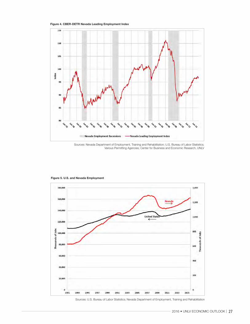
The CBER-DETR Nevada Leading Employment Index provided a clear signal by peaking in January 2006, eleven months before the CBER Nevada Coincident Employment Index reached its peak, and reached a bottom in May 2009, five months before the Nevada coincident index reached its bottom (Figure 4).

The Nevada leading employment index shows an upward pattern since its trough in May 2009. Nonetheless, its upward trek slowed in April 2014 through the present, which we also observed for the CBER Leading Index.

2. A Reemergence of Old Patterns

Prior to the Great Recession, Nevadans had grown accustomed to strong economic growth.

From January 1990 to December 2007, the latter date being when the U.S. economy peaked prior to the Great Recession, Nevada employment grew at a 4.3 percent annual rate (Figure 5). In contrast, U.S. employment grew at a 1.3 percent annual rate.

In fact, Nevada was the fastest-growing state during the 18 years prior to the Great Recession. Arizona and Utah were second and third. In general, U.S. growth was strongest in the Intermountain West, Texas, and the Southeast.

In 2014, we see a reemergence of the patterns established from 1990-2007. Growth is the fastest in North Dakota, Texas, the West, and the Southeast. For 2014, U.S. employment has grown at a rate of 2.3 percent, and Nevada is sixth with an annualized rate of 3.5 percent. Only West Virginia saw job losses.

Figure 3. CBER-DETR Nevada Coincident Employment Index


27

Figure 4. CBER-DETR Nevada Leading Employment Index


Figure 5. U.S. and Nevada Employment

Sources: U.S. Bureau of Labor Statistics; Nevada Department of Employment, Training and Rehabilitation

28

3. Economic Growth Widespread Across Nevada Economy

As shown in Figure 6, Nevada employment has been accelerating. In 2010, the state lost 7,400 jobs (0.7 percent). In 2011, 2012, and 2013, Nevada saw job gains of 12,500 (1.1 percent), 23,200 (2.1 percent) and 34,700 (3.0 percent), respectively. Growth was even stronger in 2014, with a gain of 41,200 jobs (3.5 percent). In the first nine months of 2015, the state saw job gains of 31,200 (3.4 percent annualized rate).

Of the major areas in the state, only Las Vegas mirrored the overall state pattern of gains each year (Figure 7). Reno/Sparks saw employment losses in 2011 but strengthening economic activity in 2012, 2013, 2014, and 2015, although the improvements followed a bumpy path. Carson City saw declining employment in 2011 and 2012 but employment gains in 2013 and then a fall in employment in 2014. For 2015 so far, Las Vegas, Reno/Sparks, and Carson City show strong gains. If the past provides any guidance for the future, by the end of 2015, we should expect the Las Vegas and Carson City rates to rise and Reno’s rate to fall from their current levels.

Nevada saw steady improvement from low growth in 2011, when positive job growth was first observed after the Great Recession, to stronger growth in 2015. Most industries clustered around the total employment growth in Nevada with a couple of exceptions (Figure 8). Construction, and natural resource and mining employment experienced much bigger swings in employment than either Nevada employment growth or the growth rate of the other sectors. Information showed big swings early in the sample period, but its volatility moderated in recent years. Nonetheless, employment growth was widespread across the state’s industries in 2014 and so far in 2015. In 2014, all industries except financial activities and natural resources and mining saw employment gains. Construction, leisure and hospitality, and professional and business services led the other sectors in employment growth. In the first nine months of 2015, all industries except natural resources and mining, financial services, and trade, transportation and utilities saw employment gains.

Figure 6. Nevada Employment


29

Another way to slice the data looks at the fraction of total employment in each sector (Figure 9). Leisure and hospitality employment, not surprisingly, captures the largest share of employment in Nevada at around 30 percent. The percentage in leisure and hospitality has fallen gradually from above to below 30 percent. The education and health services employment has grown from just above 5 percent to just below 10 percent. Construction’s share of total employment shows the most variability and although we noted that natural resources and mining showed much variability in its growth rate, its share of total employment in Nevada is the smallest of all sectors, along with information.

Using another way to visualize the data, we show the employment shares of the industries in September 2015 (Figure 10). To read this chart, the top item in the list on the right hand side, natural resources and mining, enters the pie chart just to the right of 12:00 on the clock face. Then, as you read down from the list on the right-hand side, you move around the clock face, clockwise.

As the result of these gains in employment, the Nevada unemployment rate has fallen. The seasonally adjusted Nevada unemployment rate is 6.7 percent (Figure 11), which is 0.7 percentage points below last year’s September unemployment rate. This decline occurred with a 32,074 increase of workers in the labor force over this time period.

Figure 7. Nevada Employment by Region, 2011-2015

Sources: U.S. Bureau of Labor Statistics; Nevada Department of Employment, Training and Rehabilitation; Center for Business and Economic Research, UNLV

30

Figure 8. Nevada Employment Growth by Industry

Figure 9. Nevada Share of Employment by Industry



31

Figure 10. Nevada Share of Employment by Industry: September 2015

Figure 11. Nevada Unemployment Rate



32

4. Nevada Reemerges as a Leader in Economic Growth

Over a nearly 25-year period from January 1990 through September 2014, including the

Great Recession, the United States saw job gains at a 1.01 percent average annual rate. Nevada employment grew nearly three times faster with an average annual rate of 2.84 percent, the highest average rate of any state in the nation during that time period.

Recessions often bring about new patterns of economic growth. Yet, for Nevada, other parts of the West, and the Southeast the current pictures are substantially similar to those before the recession. The Great Recession brought about a substantial departure from Nevada’s normal high growth rate, but the Silver State has reemerged as one of the fastest-growing states in the nation. Moreover, Nevada’s economic growth is now widespread across its industries and regions.

Since the Great Recession ended in July 2009, the total growth rate of employment for the United States was 9.2 percent. In Nevada, we grew by a

total of 10.9 percent, ranking Nevada as 11th in overall growth in employment (Figure 12). Given the boom in fracking activity, North Dakota experienced the largest growth of employment of 25.3 percent. In addition, we see that five of the larger employment growth states come from the West. West Virginia trailed the states by eking out 0.8 percent employment growth over the last six years and three months.

Employment growth leads to declining unemployment. The overall reduction in the unemployment rate since July 2009 was 4.5 percent for the United States (Figure 13). Nevada ranked 14th with a total reduction in the unemployment rate of 5.0 percent. Michigan lead the states with a total reduction in the unemployment rate of 9.7 percent, while West Virginia again trailed the states with a reduction of only 1.0 percent over the six years and three months. The Midwest and South held nine of the top 13 positions for unemployment rate reductions.

Figure 12. Employment Growth since Great Recession End

Sources: Bureau of Labor Statistics; Center for Business and Economic Research, UNLV

33

5. Annie E. Casey Foundation and Nevada KIDS COUNT

KIDS COUNT® is a well-known, well-respected project of the Annie E. Casey

Foundation (AECF). It tracks the well-being of children at both the national and the state levels and increases public awareness of the situation. All 50 states house a KIDS COUNT project, allowing for state-by-state comparisons of child well-being indicators. Projects are also located in the District of Columbia, the U.S. Virgin Islands, and the Commonwealth of Puerto Rico.

In Nevada, the primary activity of the KIDS COUNT project is to collect, analyze, and distribute the best available data measuring the educational, social, economic, and physical well-being of children and youth in Nevada. KIDS COUNT is funded by a grant to CBER.

Figure 14 reports the percent of children under age 18 in poverty by state in 2014. Nevada ranks 29th (tied with three other states) with a child poverty rate of 22 percent. This percentage equals the U.S.

average. The 12 states with the highest poverty rates cluster together with each state bordering on another high child-poverty-rate state. The states come from the Old South with Arizona and New Mexico added to the list. New Mexico ranks 50th with a child poverty rate of 30 percent, while Arizona ranks 41st (tied with four other states) with a rate of 26 percent.

Figure 15 shows the teen birth rate measured as the number of births per thousand of female teens ages 15 to 19 in 2013. Nevada ranks 32nd (tied with six other states) with a teen birth rate of 30 births per 1,000 teenage females. The U.S. rate is 26. Of the eight states with the highest teen birth rates, seven are also in the 12 states identified as the highest child-poverty-rate states. The eighth, and added, state is Oklahoma. Arizona ranks 40th with a teen birth rate of 33, while New Mexico ranks 47th (tied with two other states) with a rate of 43 per 1,000 teenage females.

Figure 13. Unemployment Rate Reduction since Great Recession End

Sources: Bureau of Labor Statistics; Center for Business and Economic Research, UNLV

34

Figure 15. Teen Birth Rates

Source: Retrieved from the Annie E. Casey Foundation, KIDS COUNT Data Center, http://datacenter.kidscount.org

Figure 14. Children in Poverty

Source: Retrieved from the Annie E. Casey Foundation, KIDS COUNT Data Center, http://datacenter.kidscount.org

35

6. Housing Market Still Recovering

The Great Recession saw more than 70 percent of home mortgages underwater at its peak.

While much progress has been made as home prices have risen in recent years, Nevada still faces a substantial issue with underwater mortgages, leading the nation in the percentage of mortgages with negative equity as well as the percentage of mortgages with negative or near negative equity (Figure 16). In the most current observation (2015 Q2), Nevada’s negative or near negative mortgages equals 23.6 percent of total mortgages. Florida and Arizona follow behind at 21.5 and 18.6 percent, respectively. Examining Nevada’s history since 2009 Q4 (Figure 17), we see that the negative or near negative equity mortgages fell from 73.0 percent in 2009 Q4 to 23.6 percent in 2015 Q2.

Figure 16. Percent Negative and Near Negative Equity Mortgages by State

Source: CORE Logic; Center for Business and Economic Research, UNLV

36

7.2 Risks to the Nevada OutlookOur outlook for the Nevada economy depends on our U.S. forecast of a slowdown in the improvement of economic conditions at the national level. This slowdown also depends on economic activity in Asia, especially China, in emerging market economies, and in European countries. We do not expect this national slowdown, however, to appreciably affect the Nevada economy. The exceptions are visitor volume and employment. The risk to the U.S. outlook provides the background on U.S. economic activity. The Nevada economy could see faster improvement in economic conditions if the U.S. economy proves stronger than we have forecast.

7. Nevada Economic Outlook

We have seen generally favorable economic trends in Nevada. We expect most of those

trends to continue in 2016 and 2017.

7.1 Nevada Economic Outlook for 2016-2017Based on our assessment of the national outlook, we believe that the Nevada economy will continue to see improvement in 2016 and 2017 (Figure 18). The gains may be stronger or weaker across the various variables based on our forecasts. Of course, each of the forecasts comes with some degree of uncertainty.

To summarize, because the Nevada economy is heavily dependent on tourism, its outlook is tied to the growth of the U.S. and western states’ economies. Southern Nevada continues to get help from real estate and construction. A wide range of industries are also growing.

Figure 17. Percent Negative and Near Negative Equity Mortgages in Nevada

Sources: CORE Logic; Center for Business and Economic Research, UNLV

37

Figure 18. Nevada Economic Outlook

Sources: Nevada Commission on Tourism; Nevada Gaming Control Board; U.S. Census Bureau; Nevada Department of Employment, Training and Rehabilitation; U.S. Bureau of Labor Statistics; U.S. Bureau of Economic Analysis;

Center for Business and Economic Research, UNLV

LEADERSHIP STARTS WITH EDUCATION

To find out more about MBA and Executive MBA programs, visit unlv.edu/mbaprograms

An MBA from UNLV isn’t just a degree. It’s a valuable tool you’ll use to transform business, to break new ground and to continually achieve new successes. You’ll learn from premier educators and scholars.

And you’ll create and sustain mutually beneficial relationships with leaders from our business community. The business world is ever-changing. Will you change with it?

EVENING MBA • Finance concentration

• Management concentration

(HR, MIS, NVM)

• Marketing concentration

EVENING MBA / DUAL DEGREE• MBA/JD (Juris Doctor)

• MBA/DMD (Doctor of Dental Medicine)

• MBA/MS (Hotel Administration)

• MBA/MS (MIS)

EXECUTIVE MBA• Designed for senior- and mid-level professionals• Accelerated 18-month schedule with classes held

every other Friday and Saturday• International Business coursework includes a capstone global experience

392016

Southern Nevada Economy to Continue Strengthening

The Southern Nevada economy continues to make steady progress towards recovery from the financial crisis and Great Recession. As of October 2015, employment in Southern Nevada was 2.0 percent below its prerecession peak. Yet, recovery is underway, and Nevada has been among the fastest-growing states in recent years.

LEADERSHIP STARTS WITH EDUCATION

To find out more about MBA and Executive MBA programs, visit unlv.edu/mbaprograms

An MBA from UNLV isn’t just a degree. It’s a valuable tool you’ll use to transform business, to break new ground and to continually achieve new successes. You’ll learn from premier educators and scholars.

And you’ll create and sustain mutually beneficial relationships with leaders from our business community. The business world is ever-changing. Will you change with it?

EVENING MBA • Finance concentration

• Management concentration

(HR, MIS, NVM)

• Marketing concentration

EVENING MBA / DUAL DEGREE• MBA/JD (Juris Doctor)

• MBA/DMD (Doctor of Dental Medicine)

• MBA/MS (Hotel Administration)

• MBA/MS (MIS)

EXECUTIVE MBA• Designed for senior- and mid-level professionals• Accelerated 18-month schedule with classes held

every other Friday and Saturday• International Business coursework includes a capstone global experience

40

1. New Indices Track Nevada Economy

As discussed in the section on the Nevada outlook, this economic outlook premiers

several new indexes that track the Nevada and Southern Nevada economies. In this section, we report information from new coincident and leading indexes of the Southern Nevada economy.

The CBER Southern Nevada Coincident Index uses the Department of Commerce index construction method to combine information on Southern Nevada taxable sales, Southern Nevada gross gaming revenue, and Southern Nevada nonfarm employment, as done for the Nevada Coincident Index. The CBER Southern Nevada Leading Index combines information on Nevada initial claims for unemployment insurance (inverted), the Moody’s real Baa interest rate (inverted), the Standard & Poor’s stock market index, Southern Nevada housing permits, Southern Nevada commercial permits, and Southern Nevada airport passengers (McCarran). The CBER Southern Nevada Coincident Index measures the ups and downs of the Southern Nevada economy. The CBER Southern Nevada Leading Index also measures the ups and downs of the Southern Nevada economy, providing a signal about the future direction of the coincident index. The coincident index provides the benchmark series that defines the business cycle or reference cycle in Southern Nevada. The leading index then tracks the economy relative to that reference cycle. A good leading index will provide signals about the future path of the reference cycle.1

The coincident index includes three full recessions and the bulk of a fourth recession in the early 1980s (Figure 1). The financial crisis and Great Recession generated the longest and deepest of these four recession episodes. The index peaked in February 2007 and then fell dramatically through June 2010, an almost three and one-half year period of decline. These dates match exactly the peak to trough in the Great Recession in the CBER Nevada Coincident Index. Currently, the index has recovered almost 99 percent of its

1. All series are initially not seasonally adjusted and then seasonally adjusted using Census X12.

decline during the Great Recession. It took just over five years to achieve this level of recovery.

Prior to the Great Recession identified by the benchmark Southern Nevada coincident index, the Southern Nevada leading index peaked in September 2005, 16 months before the Nevada coincident index peaked (Figure 2). Then the Nevada leading index troughed in May 2009, 13 months before the Southern Nevada coincident indexed troughed. Unlike the CBER Nevada Leading Index, the two earlier recessions in the early 1990s and early 2000s, the leading index did turn before the coincident index at both the peaks and troughs of the cycle. Finally, for the first cycle in the early 1980s, the leading index peaked in January 1980, 19 months before the Nevada coincident indexed peaked in August 1981. Then the leading indexed troughed in April 1982, seven months before the Southern Nevada coincident index troughed in November 1982. The leading index still looks like it follows an upward trajectory, although, the upward movement moderated beginning in July 2014.

41

Figure 1. CBER Southern Nevada Coincident Index

Sources: Nevada Gaming Control Board; Nevada Department of Taxation; Nevada Department of Employment, Training and Rehabilitation; U.S. Bureau of Labor Statistics; Center for Business and Economic Research, UNLV

Figure 2. CBER Southern Nevada Leading Index

Sources: McCarran International Airport; Various Permitting Agencies; Nevada Department of Employment, Training and Rehabilitation; U.S. Bureau of Labor Statistics; Yahoo Finance; Federal Reserve Bank of St. Louis;

Center for Business and Economic Research, UNLV

42

The Southern Nevada economy is continuing to experience growth (Figure 3). Although the annualized growth rate for 2015 is down from the growth rates for 2014 for Las Vegas, Nevada employment growth in 2015 exceeds that for 2014. These annualized numbers still have a couple of months of additional data and they may be revised upward next March, as it has been the norm over the last few years. In addition to strong employment gains, financial conditions also are improving, and visitor volume is still rising after a strong 2014.

Las Vegas still has a ways to go before it reaches its prerecession level of economic activity, but that gap is closing. As far as employment is concerned, that goal is within sight; we can expect Las Vegas to reach its prerecession levels of employment in early 2016.

2. Southern Nevada Economic Conditions Improving

In 2014, the Las Vegas metropolitan area saw an increase in employment of 32,600 jobs (3.9

percent) over the previous year (Figure 4). In the first nine months of 2015, the Las Vegas metropolitan area saw another increase in employment of 18,800 jobs (at a 2.5 percent annual rate). Overall, the Las Vegas and Nevada employment trends tend to move in synchronization.

Taxable sales continue to be strong (Figure 5). Clark County taxable sales were 8.0 percent higher year-over-year in July 2015. Increased visitor spending and rising personal income in Las Vegas are two factors contributing to the strong gains in taxable sales. The most recent trend of 6.2 percent annual growth rate in taxable sales falls a bit below the trend in the 1980s of 10.3 percent, the 1990s of 10.0 percent, and the 2000s before the Great Recession of 9.2 percent.

Figure 3. Nevada and Las Vegas Job Growth

Sources: Nevada Department of Employment, Training and Rehabilitation; U.S. Bureau of Labor Statistics; Center for Business and Economic Research, UNLV

43

Figure 4. Nevada and Las Vegas Employment

Sources: Nevada Department of Employment, Training and Rehabilitation; U.S. Bureau of Labor Statistics

Figure 5: Clark County Taxable Sales

Sources: Nevada Department of Taxation; Center for Business and Economic Research, UNLV

44

Gross gaming revenue always shows volatility, but the volatility increases sharply after the Great Recession (Figure 6). Note that the gross gaming revenue is seasonally adjusted, but still experiences high volatility. In addition, the drop in gross gaming revenue during the Great Recession dwarfs the prior recessions in the chart. For the first nine months of 2015, Clark County gaming revenue fell by 2.2 percent on a year-over-year basis.

As we also saw for the Nevada economy, most sectors track the growth rate of total employment rather closely with some notable exceptions (Figure 7). Construction and information follow a more volatile path than total employment. Construction and professional and business services are growing the most rapidly in 2015 with annualized rates of 13.2 and 5.9 percent, respectively. Financial activities and trade, transportation, and utilities are shedding jobs at rates of -0.5 and -6.1 percent, respectively.

The share of employment by sector provides a different way to examine sectoral employment data (Figure 8). We see that leisure and hospitality employment fell from about 35 percent to just over 30 percent of total employment. The trade, transportation, and utilities sector keeps a steady share of total employment of around 17 to 18 percent. This represents about a 5 percent larger share of total employment in Southern Nevada as compared to the whole state. Education and health services rose in Las Vegas from around 5 to 10 percent, matching a similar movement at the state level. We do not include natural resources and mining as its share of total employment is negligible in Southern Nevada. We also notice some increase in professional and business services as a fraction of total employment in Las Vegas.

Figure 6: Clark County Gross Gaming Revenue

Sources: Nevada Gaming Control Board; Center for Business and Economic Research, UNLV

45

Figure 7. Las Vegas Employment Growth by Industry


Figure 8. Las Vegas Share of Employment by Industry

Sources: U.S. Bureau of Labor Statistics; Nevada Department of Employment, Training and Rehabilitation; Center for Business and Economic Research, UNLV; Federal Reserve Bank of St. Louis

46

Figure 9 reports the distribution of jobs by sector in September 2015. To read this chart, the top item in the list on the right hand side, construction, enters the pie chart at the 12:00 to 1:00 time slot on the clock face. Then, as you read down from the list on the right-hand side, you move around the clock face clockwise.

As the result of these gains, the Las Vegas unemployment rate has fallen sharply. The seasonally adjusted Las Vegas unemployment rate is 6.8 percent (Figure 10), which is 0.3 percentage points below last year’s December unemployment rate. This decline in the unemployment rate occurred even though the labor force increased by 25,900 persons over the same time period.

3. Tourism and Gaming

Activity in the tourism sector, as measured by CBER’s Clark County Tourism Index, shows

a slight upward trend for 2015 thus far (Figure 11). The index is composed of three components—Clark County gross gaming revenues, the Las Vegas hotel/motel occupancy rate, and total passengers enplaned/deplaned at McCarran International Airport. We employ the Department of Commerce method to construct this and the other indexes that follow in this section. The recessions correspond to the benchmark series for Las Vegas, the Southern Nevada Coincident Index. Compared to the other recessions in Las Vegas, with the exception of 9/11 drop, the Great Recession caused a sharp drop in the Clark County Tourism Index. The recovery from the bottom of the Great Recession has been slow but steady. The index has yet to pass its previous peak, although that should occur in the not too distant future.

Figure 9. Las Vegas Share of Employment by Industry: September 2015


47

Figure 10. Las Vegas Unemployment Rate

Sources: Nevada Department of Employment, Training and Rehabilitation; U.S. Bureau of Labor Statistics; Federal Reserve Bank of St. Louis

Figure 11. Clark County Tourism Index

Sources: Nevada Gaming Control Board; Las Vegas Convention and Visitors Authority; McCarran International Airport; Center for Business and Economic Research, UNLV

48

McCarran passenger volume has recently begun to grow at a brisk pace (Figure 12), generating a 16.2 percent increase year over year in August 2015. The growth rate of McCarran passengers equaled -0.8, 4.1, and 1.9 percent in 2012, 2013, and 2014, respectively. Thus, the recent movements in the number of passengers going through McCarran Airport represent a much needed boost in airport traffic.

As shown in Figure 13, Clark County hotel occupancy rates have risen since the end of the Great Recession. They now run at between 85 and 90 percent, which nearly returns Las Vegas to its normal range, since the early 1990s.

4. Construction Activity

Activity in the construction sector, as measured by CBER’s Clark County Construction

Index, shows a significant upward trend since January 2012 (Figure 14). The index is composed of three components—Clark County construction employment, Clark County residential permits, and Clark County commercial permits. The recessions, once again, correspond to the benchmark series for Las Vegas, the Southern Nevada Coincident Index. Compared to the other recessions in Las Vegas, the Great Recession caused a dramatic drop in the Clark County Construction Index. The recovery from the bottom of the Great Recession was delayed for some time, but has taken off since January 2013. Of course, we do not see a return to the heights of the index during the boom in construction activity, leading up to the financial crisis and Great Recession.

Figure 12. McCarran Passengers

Sources: McCarran International Airport; Center for Business and Economic Research, UNLV

49

Figure 13. Clark County Hotel Occupancy

Sources: Las Vegas Convention and Visitors Authority; Center for Business and Economic Research, UNLV

Figure 14. Clark County Construction Index

Sources: Various Permitting Agencies; Nevada Department of Employment, Training and Rehabilitation; U.S. Bureau of Labor; Center for Business and Economic Research, UNLV

50

Clark County housing permits took a deep dive during the financial crisis and Great Recession (Figure 15), falling to levels not seen since the early 1980s. The drop went from around 4,000 permits per month to about 500 permits per month. Since the end of the Great Recession, housing permits have rebounded at a pace similar to the early 1980s, now standing at nearly 1,000 permits per month.

Clark County commercial permits also took a deep dive during the financial crisis and Great Recession (Figure 16), falling to levels even lower than the early 1980s. The drop went from around 125 permits per month to about 25 permits per month. Since the end of the Great Recession, commercial permits in Clark County have risen ever so slightly.

Clark County construction employment also took a big dive during the financial crisis and Great Recession (Figure 17), falling from around 125,000 workers to under 40,000 workers in early 2012. Unlike housing and commercial permits, the fall did not take construction employment back to levels in the early 1980s but rather back to

levels in the early 1990s. Since then, construction employment has recovered to just over 50,000 workers.

The bursting of the housing bubble, which began in late 2006, led to the Great Recession. The declining home prices after the bursting of the bubble made homes more affordable. The housing opportunity index measures the affordability of homes. The index captures the percent of homes sold that are affordable at the median income. If the housing market is balanced in terms of affordability, then the median income household should be able to purchase the median-priced home in the market. Thus, the index would equal 50 percent.

Figure 15. Clark County Housing Permits

Sources: Various Permitting Agencies; Center for Business and Economic Research, UNLV

51

Figure 16. Clark County Commercial Permits

Sources: Various Permitting Agencies; Center for Business and Economic Research, UNLV

Figure 17. Clark County Construction Employment


52

The housing opportunity index (Figure 18) shows that the Las Vegas and Phoenix housing markets have tracked solely to the U.S. index since late 2012. In 2015 Q3, these two indices popped above the U.S. index. The California market, as represented by Los Angeles and Riverside, is trending downward more quickly than the U.S. index. Los Angeles and Riverside stand at opportunity indices of 14.7 and 41.0, respectively, in 2015 Q3, much below the U.S. index of 62.2. During the end of the bubble in 2006, Los Angeles and Riverside averaged 1.9 and 7.3 percent, respectively, on the opportunity index. Las Vegas and Phoenix averaged 15.6 and 28.8, respectively, in 2006. The U.S. average was 41.0.

In sum, the Las Vegas housing market remains relatively affordable, as does the Phoenix market.

5. Annie E. Casey Foundation and Nevada KIDS COUNT

This section extends the discussion of Nevada KIDS COUNT begun in the section on the

Nevada outlook. Here, we consider the same two measures of children’s wellbeing, but for the various counties in Nevada.

Figure 19 shows the percentage of children in poverty by county in Nevada in 2013. We see that the highest rates appear in Southern Nevada in Mineral and Nye counties with child poverty rates of 30.2 and 31.6 percent, respectively. Clark County ranks 13th with a rate of 23.7 percent. The child poverty rate for Nevada is 22.7 percent.

Figure 20 reports the teen birth rate per 1,000 females in the age range 15 to 19 over the 2011-2013 time period. The highest rates appear in Northern Nevada in Lander, Pershing, and Humboldt counties with teen birth rates of 37.7, 38.5, and 45.5 per 1,000 teenage females, respectively. Clark County ranked 7th with a rate of 32.1. Nevada’s rate is 31.5 per 1,000 teenage females. Note that because of fewer than 10 births over the three-year period, Lincoln, Eureka, and Storey counties are not reported separately.

Figure 18. Housing Opportunity Index

Sources: National Association of Home Builders and Wells Fargo

53

Figure 19. Children in Poverty

Source: U.S. Census Bureau, Small Area Income and Poverty Estimates (SAIPE) Program

Figure 20. Teen Birth Rates

Source: Nevada Department of Health and Human Services, Nevada Division of Public and Behavioral Health, Office of Public Health Informatics and Epidemiology

54

The distribution of responses by number of employees shows a large component of small businesses (Figure 22). The largest firms with more than 250 employees only constitute 22.5 percent of our overall sample of firms.

When asked about the most important problem faced by the firm as a result of the financial crisis, the respondents gave a number of different responses (Figure 23). The most responses, mentioned by 46.1 percent of the respondents, chose the unpredictability of business conditions. The role of uncertainty probably plays an important part in the unwillingness of firms to make new investment and to hire new workers, fearing that a bad turn of events that is unexpected could jeopardize the viability of the firm. Next, respondents listed the slowness or loss of sales as an important problem.

6. Southern Nevada Business Confidence Index

CBER’s Southern Nevada Business Confidence Index also provides a favorable picture (Figure

21). Although some seasonality appears to exist in the index, the index reached a post-recession high of 148.1 in the first quarter of 2015. Since then, the index fell for three consecutive quarters, finishing in the fourth quarter of 2015 at 122.6. Any value above 100 means that more respondents are optimistic about the outlook for business conditions than are pessimistic. Thus, we still lie well above the dividing line between optimism and pessimism.

The index consists of five components—business expectations for sales, profits, hiring, capital investment, and overall economic conditions—all of which are measured by a survey of Southern Nevada business leaders. For fourth quarter of 2015, all five components were above 100.

Figure 21. CBER Southern Nevada Business Confidence Index

Source: Center for Business and Economic Research, UNLV

55

Figure 22. Respondents by Number of Employees


Figure 23. Most Important Problem Faced because of the Financial Crisis


56

When asked about the most serious long-term problem emanating from the financial crisis, 38.3 percent of the respondents chose the long period of no or slow economic growth (Figure 24). This long-term problem connects to the previous question in that no or slow growth is a probable outcome of unpredictable business conditions that contributed to an unwillingness to invest in and hire new workers.

7. Southern Nevada Economic Outlook for 2016 and 2017

Based on our assessment of national and Nevada trends in 2016 and 2017, we believe

that the Southern Nevada economy will continue to see improvement in 2016 and 2017 (Figure 25).

7.1 Nevada Economic Outlook for 2016-2017We believe that the Southern Nevada economy will continue to see improvement in 2016 and 2017. The gains should be stronger or weaker across the various variables based on our forecasts. Of course, each of the forecasts comes with some degree of uncertainty.

To summarize, because the Southern Nevada economy is heavily dependent on tourism, its outlook is tied to the growth of the U.S. and western states’ economies. Southern Nevada continues to get help from real estate and construction. A wide range of industries are also growing.

7.2 Risks to the Southern Nevada Economic OutlookThe Southern Nevada outlook depends on our forecast of slowing economic growth in 2016 at the national level. This national slowdown also depends on economic activity in Asia, especially China, in emerging market economies, and in European countries. Nevertheless, the outlook suggests that the small slowdown at the national level will not affect the Southern Nevada economy by any large amount. The risk to the U.S. outlook provides the background on U.S. economic activity. The Nevada economy could see faster improvement in economic conditions if the U.S. economy proves stronger than we have forecast.

Figure 24. Most Serious Long-Term Problem Coming Out of the Financial Crisis


57

Figure 25. Southern Nevada Economic Outlook

Sources: Las Vegas Convention and Visitors Authority; Nevada Gaming Control Board; Standard & Poor’s; Various Permitting Agencies; Nevada Department of Employment, Training and Rehabilitation; U.S. Bureau of Labor

58

CBER’s Long-Term Forecast for the Southern Nevada Population

Each year, the Regional Transportation Commission (RTC), the Southern Nevada Water Authority (SNWA), the Southern Nevada Regional Planning Coalition (SNRPC), the Center for Business and Economic Research (CBER) at the University of Nevada, Las Vegas, and a group of community demographers and analysts work together to provide a long-term forecast of economic and demographic variables influencing Clark County. The primary goal is to develop a long-term forecast of the Clark County population that is consistent with the structural economic characteristics of the county. Toward this end, we employ a general-equilibrium demographic and economic model developed by Regional Economic Models, Inc. (REMI), specifically for Clark County.

1. The REMI Model

The REMI model is a state-of-the-art econometric forecasting model that accounts for dynamic

feedbacks between economic and demographic variables. Special features allow the user to update the model to include the most current economic information. CBER calibrates the model using information on recent local employment levels, the most recent national Gross Domestic Product (GDP) forecast, spending on local capital projects, and adjustments for amenities related to local population growth.

The model employed divides Nevada into five regions: Clark County, Nye County, Lincoln County, Washoe County, and the remaining counties, which are combined to form a fifth region. These regions are modeled using the U.S. economy as a backdrop. The model contains over 100 economic and demographic relationships that are carefully constructed to concisely represent the Clark County economy. The model includes equations to account for migration and trade between Nevada counties and other states and counties in the country.

1.1 Recalibrating the ModelThe economic data for the most recent version of the model (REMI PI+ v1.6) are consistent with the

North American Industry Classification System (NAICS). The most recent data for REMI PI+ v1.6 are from 2012 because the Bureau of Labor Statistics (BLS) personal-income data are reported with a two-year lag. Over the years, the availability of the income data has been the key in setting the last year of history in the model. To guarantee that the most current data are used in the forecast, we make a series of adjustments to the model. In this way, we ensure that the forecast model includes the best available information at the time the forecast is made.

1.1.1 Adjustment of the national GDP forecastThe REMI model relies on a baseline national GDP forecast from the University of Michigan’s Research Seminar in Quantitative Economics (RSQE). The current REMI model, PI+ v1.6, utilizes the March 2014 GDP forecast from RSQE. We adjust the model’s national GDP forecast using the March 2015 national GDP forecast from RSQE. Overall, we adjusted the national GDP components downward by about $105 billion in 2015 and $137 billion in 2016. The adjusted national forecast is used to generate a new baseline forecast for Clark County. The baseline forecast is then used for the subsequent adjustments.

1.1.2 Employment adjustmentOne of the most noteworthy updates we make to the REMI model is the employment adjustment. The industry-level employment data used by REMI are the sum of the BLS wage and salary estimates for Clark County and REMI’s BLS-based estimate of the number of proprietors. The most recent historical year in the model data is 2012. However, more recent wage and salary employment data are available from the Nevada DETR for 2013 and 2014. Thus, we update the model to account for the more recent information.

1.1.3 Transportation and infrastructure improvementsClark County has continued to invest in transportation infrastructure such as roads, highways, and mass transit. The model assumes that public-infrastructure investment will continue at a pace consistent with the model history. Thus,

59

some local spending on public infrastructure, such as road building and additional services, is built into the model. However, one-time monies tend to come from outside the region (for example, federal transportation funding). These large, special projects need to be accounted for in the forecast.

1.1.4 Rebasing the population forecastWe rebase the population forecasts using the population update feature in the REMI model. We update the population in 2014 based on the most recent information available for use from the SNRPC. The SNRPC consensus population estimate for Clark County in 2014 is 2.1 million. In addition, we update the population levels in 2015 and 2016 to reflect the population growth-rate forecast from CBER’s 2015 Economic Outlook, which was published in December 2014. The latter adjustment is intended to incorporate the views of local economic experts at CBER in the short-term population forecasts. CBER predicts that the Clark County population will grow by 2.1 percent in 2015 and 2016. These population growth-rate forecasts translate to a forecasted population of 2.15 million in 2015 and 2.19 million in 2016. We use these forecasted population levels to update the population in the REMI model.

2. Analysis of the Population Forecast

In the short term, the current forecast predicts moderate rates of population growth in

Southern Nevada. The population in Clark County is predicted to grow at a rate of 2.1 percent in 2015 and 2016. The population growth rate declines in the medium term as the Clark County economy moves closer to maturity. By 2030, the population growth rate falls to 1.1 percent as the Clark County economy is expected to mature; and it reaches 0.7 percent, slightly above the projected1 long-term national population growth rate of 0.5 percent, by 2050. This pattern of long-term growth is expected as our economy matures and is very similar to previous forecasts.

Clark County is forecasted to add roughly 44,000 new residents in 2015. CBER’s 2015 Southern Nevada Economic Outlook predicts that population growth will strengthen with employment in the near term, and it will not be a driver of economic growth as it was throughout much of Las Vegas’ history. Rather, economic growth will drive population in the next few years.

1. Source: http://www.census.gov/population/projections/data/national/2014.html

Figure 1. Clark County Population Forecast

Sources: Clark County Comprehensive Planning and Center for Business and Economic Research, UNLV

60

The population forecast predicts that the Clark County population will be roughly 3.11 million by 2050.

3. Risks to the Forecasts

Our Southern Nevada population forecasts rest on economic and demographic models

set in the context of a structured framework. This structure keeps our long-term forecasts consistent with our objectives. We have separated the long-term trend from the noise that one finds in time-series data. These noise factors include the business cycle and seasonal and irregular events.

The main risks to the population forecasts arise from short-term fluctuations in both U.S. and Southern Nevada economic conditions. Based on our assessment of the national and regional trends, we believe that the Southern Nevada economy will continue to see improvements in 2015 and 2016. This outlook for the Southern Nevada economy is based on the idea that improving economic conditions in the United States, particularly in the West, will benefit the Southern Nevada economy. As the growth of the U.S. economy accelerates, the Southern Nevada economy will further strengthen. This would result in higher population growth rates than those we are seeing in the current forecast. The Southern Nevada economy could see slower growth if the U.S. economy proves weaker than we have predicted. This would result in lower population growth rates than those we are seeing in the current forecast.

Therefore, although we feel the population forecasts are sound, there are significant risks to the forecasts that could lead to either over- or underestimated growth. We say again, however, that these risks tend to arise from short-term uncertainty; whereas, our forecasts are primarily meant to be long-term planning tools.

Welcome to the Nevada Gaming

Compensation Survey Conducted by WageWatch

THE LEADER IN SALARY SURVEYS FOR THE GAMING INDUSTRY

• Receive wage and salary data on over 250 key positions

• Create custom reports by comparing to other NV casinos

• Generate unlimited reports 24/7, year round

• Retain the brightest talent and keep turnover low

• Access wage and salary data for the following departments:

• Administrative

• Sales/Marketing

• Bingo

• Cage

• Credit

• Collections

• Card Room

• Casino

• Communications

• Technology

• Surveillance

• Slots

• Engineering

• Finance

• Food and Beverage

• Hotel

• Housekeeping

• Human Resources

• Kitchen

• Security

• Property Maintenance

• Spa

1.888.330.WAGE (9243) ▪ www.wagewatch.com

economic outlook 20162016 1 u.s. economy continues to show moderate growth the current macroeconomic...

Documents