economic model predictive control - research unit...
TRANSCRIPT
Economic model predictive control
Pantelis Sopasakis
IMT institute for Advanced Studies Lucca
February 2, 2016
Outline
X Economic MPC – Introduction and basic properties
X Dissipativity
X Stability
X Terminal cost and constraints
X Asymptotic average constraints
1 / 71

I. Introduction to EMPC
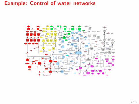
Example: Control of water networks
2 / 71

Example: Control of water networks
Control objectives:
1. Economic operation
2. Smoothness of control actions
3. Maintenance of a safety volume in each reservoir
4. Satisfaction of constraints
5. Stability
3 / 71

Example: Control of water networks
20 40 60 80 100 120 140 160
Re
ple
tio
n [
%]
0
20
40
60
80
100
Closed-loop MPC Simulation
Time [hr]
20 40 60 80 100 120 140 160
De
ma
nd
[m
3/s
]
0
0.5
1
1.5
2
4 / 71
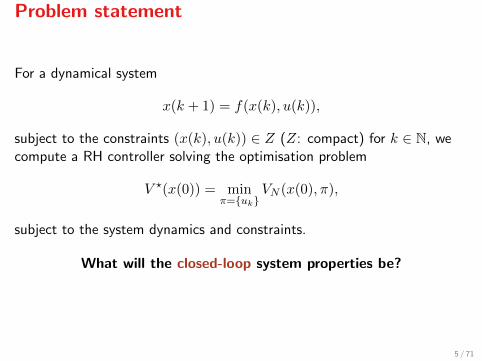
Problem statement
For a dynamical system
x(k + 1) = f(x(k), u(k)),
subject to the constraints (x(k), u(k)) ∈ Z (Z: compact) for k ∈ N, wecompute a RH controller solving the optimisation problem
V ?(x(0)) = minπ={uk}
VN (x(0), π),
subject to the system dynamics and constraints.
What will the closed-loop system properties be?
5 / 71
Problem statement
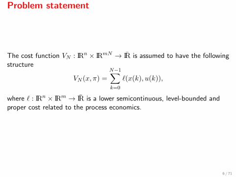
The cost function VN : IRn × IRmN → IR is assumed to have the followingstructure
VN (x, π) =
N−1∑k=0
`(x(k), u(k)),
where ` : IRn × IRm → IR is a lower semicontinuous, level-bounded andproper cost related to the process economics.
6 / 71
Stage cost
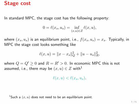
In standard MPC, the stage cost has the following property:
0 = `(xs, us) = inf(x,u)∈Z
`(x, u),
where (xs, us) is an equilibrium point, i.e., f(xs, us) = xs. Typically, inMPC the stage cost looks something like
`(x, u) = ‖x− xs‖2Q + ‖u− us‖2R,
where Q = Q′ ≥ 0 and R = R′ > 0. In economic MPC this is notassumed, i.e., there may be (x, u) ∈ Z with1
`(x, u) < `(xs, us).
1Such a (x, u) does not need to be an equilibrium point.
7 / 71
Stage cost
In economic MPC, the stage cost ` reflects the process economics,not a control objective.
8 / 71
Optimal steady states
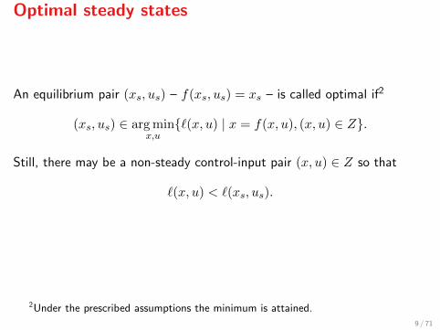
An equilibrium pair (xs, us) – f(xs, us) = xs – is called optimal if2
(xs, us) ∈ arg minx,u
{`(x, u) | x = f(x, u), (x, u) ∈ Z}.
Still, there may be a non-steady control-input pair (x, u) ∈ Z so that
`(x, u) < `(xs, us).
2Under the prescribed assumptions the minimum is attained.
9 / 71
EMPC formulation
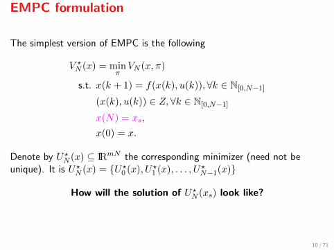
The simplest version of EMPC is the following
V ?N (x) = min
πVN (x, π)
s.t. x(k + 1) = f(x(k), u(k)),∀k ∈ N[0,N−1]
(x(k), u(k)) ∈ Z, ∀k ∈ N[0,N−1]
x(N) = xs,
x(0) = x.
Denote by U?N (x) ⊆ IRmN the corresponding minimizer (need not beunique). It is U?N (x) = {U?0 (x), U?1 (x), . . . , U?N−1(x)}
How will the solution of U?N (xs) look like?
10 / 71
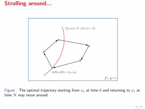
Strolling around...
Figure : The optimal trajectory starting from xs at time 0 and returning to xs attime N may move around.
11 / 71
Some definitions
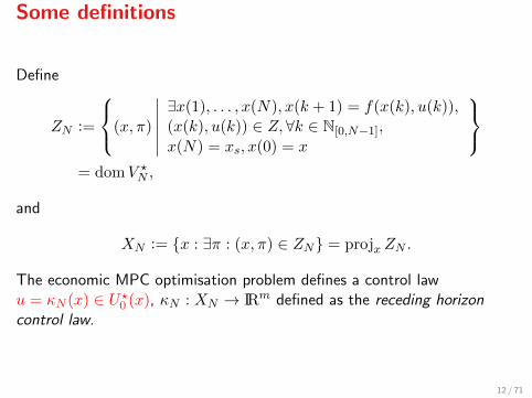
Define
ZN :=
(x, π)
∣∣∣∣∣∣∃x(1), . . . , x(N), x(k + 1) = f(x(k), u(k)),(x(k), u(k)) ∈ Z, ∀k ∈ N[0,N−1],
x(N) = xs, x(0) = x
= domV ?
N ,
and
XN := {x : ∃π : (x, π) ∈ ZN} = projx ZN .
The economic MPC optimisation problem defines a control lawu = κN (x) ∈ U?0 (x), κN : XN → IRm defined as the receding horizoncontrol law.
12 / 71

Assumptions
We shall always assume that
1. Functions f : Z → IRn and ` : Z → IR are continuous,
2. xs ∈ intXN
3. There exists a K∞-class function γ : IRn → IR+ such that forx ∈ XN there is a π with (x, π) ∈ Z so that
‖π − (us, us, . . . , us)′‖ ≤ γ(‖x− xs‖).
4. Z is a compact nonempty set
13 / 71

Control invariance of XN
XN is control invariant.
Proof.Take x(0) = x ∈ XN ; there is π such that (x, π) ∈ ZN
π = (u0, u1, . . . , uN−1),
then choose π be π = (u1, . . . , uN−1, us), so that for x(1) = f(x, u0), π isa feasible sequence, thus x(1) ∈ XN .
14 / 71
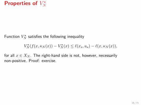
Properties of V ?N
Function V ?N satisfies the following inequality
V ?N (f(x, κN (x))− V ?
N (x) ≤ `(xs, us)− `(x, κN (x)),
for all x ∈ XN . The right-hand side is not, however, necessarilynon-positive. Proof: exercise.
15 / 71
Caveats...
Since it is not assumed that τ(x) := `(xs, us)− `(x, κN (x)) ≺ 0,
1. {V ?N (xk)}k may not be monotonically decreasing,
2. The ∞-horizon cost may diverge,
3. V ?N (·) is not a Lyapunov function for the c/l system.
16 / 71
Closed-loop asymp. average performance
To assess the performance of the closed-loop system we introduce thefollowing index:
J(κN ) := lim supT→∞
∑Tk=0 `(x(k), κN (x(k)))
T + 1,
which is called asymptotic average cost.
17 / 71

Performance bounds
The EMPC-controlled system has an asymptotic average performance thatis no worse than that of the best admissible steady state.
18 / 71
Performance bounds
The following performance bound holds:
J(κN ) ≤ `(xs, us).
Proof.Hint: use V ?
N (x+)−V ?N (x)≤`(xs, us)−`(x, u), take as. averages on both
sides. Assume – without loss of generality – that `(x, u) ≥ 0 over ZN .
Note. this bound holds only for the as. average cost, i.e., for any given Twe cannot prove that ∑T
k=0 `(x(k), κN (x(k)))
T + 1,
is bounded by `(xs, us).
19 / 71
End of first section
Conclusions.
1. Stability is not always in question
2. The stage cost ` may reflect an economic or performance objective
3. We studied a simple EMPC formulation with x(N) = xs
4. for which Recursive feasibility is guaranteed
5. Perfomance is quantified using the asymptotic average cost
6. which is bounded above by the steady-state operation as. aver. cost.
20 / 71
II. Dissipativity
Dissipativity
A control system is called dissipative3 with respect to a supply rates : Z → IR, Z ⊆ IRn+m, if there exists a function λ : IRn → IR such thatfor all (x, u) ∈ Z
λ(f(x, u))− λ(x) ≤ s(x, u).
If, additionally, there is a pos. def. function ρ : IRn → IR so that for all(x, u) ∈ Z
λ(f(x, u))− λ(x) ≤ −ρ(x) + s(x, u),
then the control system is called strictly dissipative.
3Dissipativity is for open-loop systems what stability is for closed-loop ones.
21 / 71
Dissipativity
Often we use the following supply rate
s(x, u) = `(x, u)− `(xs, us).
Then, the system is dissipative if
λ(f(x))− λ(x) ≤ `(x, u)− `(xs, us)⇔`(x, u) + λ(x)− λ(f(x, u)) ≥ `(xs, us)⇔ min
(x,u)∈Z[`(x, u) + λ(x)− λ(f(x, u))] ≥ `(xs, us)
It will be useful to define the rotated stage cost
L(x, u) := `(x, u) + λ(x)− λ(f(x, u)).
22 / 71
* A little detail
On the pervious slide the following optimisation problem was formulated:
min(x,u)∈Z
[`(x, u) + λ(x)− λ(f(x))] .
But, is the min attained for any functions ` and λ?
The answer is affirmative when L(x, u) is lsc, level-bounded (alllevel-sets are bounded) and proper.
23 / 71
* A little detail
On the pervious slide the following optimisation problem was formulated:
min(x,u)∈Z
[`(x, u) + λ(x)− λ(f(x))] .
But, is the min attained for any functions ` and λ?
The answer is affirmative when L(x, u) is lsc, level-bounded (alllevel-sets are bounded) and proper.
23 / 71
Dissipativity
Notice that
min(x,u)∈Z
L(x, u) ≤ min(x,u)∈Zx=f(x,u)
L(x, u)
= min(x,u)∈Zx=f(x,u)
`(x, u) = `(xs, us)
Dissipativity holds when:
min(x,u)∈Z
L(x, u) ≥ min(x,u)∈Zx=f(x,u)
`(xs, us).
24 / 71
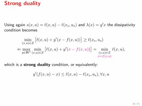
Strong duality
Using again s(x, u) = `(x, u)− `(xs, us) and λ(x) = y′x the dissipativitycondition becomes
min(x,u)∈Z
[`(x, u) + y′(x− f(x, u))
]≥ `(xs, us)
⇐ maxy∈IRn
min(x,u)∈Z
[`(x, u) + y′(x− f(x, u))
]= min
(x,u)∈Zx=f(x,u)
`(x, u),
which is a strong duality condition, or equivalently:
y′(f(x, u)− x) ≤ `(x, u)− `(xs, us),∀x, u
25 / 71
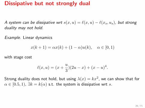
Dissipative but not strongly dual
A system can be dissipative wrt s(x, u) = `(x, u)− `(xs, us), but strongduality may not hold.
Example. Linear dynamics
x(k + 1) = αx(k) + (1− α)u(k), α ∈ [0, 1)
with stage cost
`(x, u) = (x+u
3)(2u− x) + (x− u)4.
Strong duality does not hold, but using λ(x) = kx2, we can show that forα ∈ [0.5, 1), ∃k = k(α) s.t. the system is dissipative wrt s.
26 / 71

End of second section
Conclusions.
1. Dissipativity is the open-loop counterpart of stability
2. When min(x,u ∈ S`(x, u) is str. dual, then we have dissipativity wrts(x, u) = `(x, u)− `(xs, us)
3. Absense of strong duality does not mean that the system is notdissipative wrt s
4. We defined the rotated cost L(x, u) = `(x, u) + λ(x)− λ(f(x, u))which will come in handy later
5. We’ll use a strong dissipativity assumption to prove stability
27 / 71
III. Asymptotic stability
Asymptotic stability
Under what conditions is xs an asymptotically stable equilibrium point forthe EMPC-controlled system?
To answer this question we introduce the following auxiliary cost function:
VN (x, π) =N−1∑k=0
L(x(k), u(k)).
and we formulate the auxiliary EMPC problem
V ?N (x) = min
πVN (x, π),
subject to the same constraints.
28 / 71

Asymptotic stability
Under what conditions is xs an asymptotically stable equilibrium point forthe EMPC-controlled system?
To answer this question we introduce the following auxiliary cost function:
VN (x, π) =
N−1∑k=0
L(x(k), u(k)).
and we formulate the auxiliary EMPC problem
V ?N (x) = min
πVN (x, π),
subject to the same constraints.
28 / 71
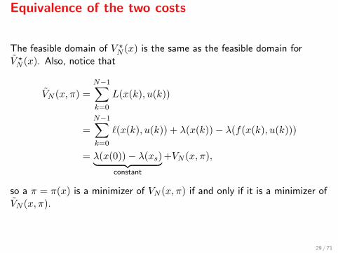
Equivalence of the two costs
The feasible domain of V ?N (x) is the same as the feasible domain for
V ?N (x). Also, notice that
VN (x, π) =
N−1∑k=0
L(x(k), u(k))
=
N−1∑k=0
`(x(k), u(k)) + λ(x(k))− λ(f(x(k), u(k)))
= λ(x(0))− λ(xs)︸ ︷︷ ︸constant
+VN (x, π),
so a π = π(x) is a minimizer of VN (x, π) if and only if it is a minimizer ofVN (x, π).
29 / 71

Asymptotic stability condition
Let (xs, us) be an optimal equilibrium point. If the control system isstrictly dissipative wrt s(x, u) = `(x, u)− `(xs, us) then xs is anasymptotically stable equilibrium point for the EMPC-controlled systemwith region of attraction XN .
Proof.Use the equivalence between V ?
N and V ?N and the definition of strict
dissipativity to show that V ?N (x+)− V ?
N (x) ≤ −ρ(x) for x ∈ XN .
30 / 71
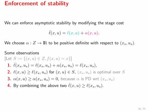
Enforcement of stability
We can enforce asymptotic stability by modifying the stage cost
¯(x, u) = `(x, u) + α(x, u).
We choose α : Z → IR to be positive definite with respect to (xs, us).
Some observations[Let S := {(x, u) ∈ Z, f(x, u) = x}]
1. ¯(xs, us) = `(xs, us) + α(xs, us) = `(xs, us),
2. `(x, u) ≥ `(xs, us) for (x, u) ∈ S, (xs, us) is optimal over S
3. α(x, u) ≥ α(xs, us) = 0, because α is PD wrt (xs, us)
4. By combining the above two ¯(x, u) ≥ `(xs, us).
31 / 71

Enforcement of stability
To achieve strict dissipativity wrt s(x, u) = ¯(x, u)− ¯(xs, us) thefollowing needs to hold (we choose λ(x) = y′x)
λ(f(x))− λ(x) ≤ −ρ(x) + s(x, u)
⇔ y′(f(x, u)− x) ≤ −ρ(x) + ¯(x, u)− ¯(xs, us)
⇔ y′(f(x, u)− x) ≤ −ρ(x) + `(x, u) + α(x, u)− `(xs, us)⇔ α(x, u) ≥ ρ(x) + `(xs, us) + y′(f(x, u)− x)− `(x, u)
⇔ α(x, u) ≥ h(x, u, y).
Now for r ≥ 0 define
H(r, y) := maxx,u{h(x, u, y) | (x, u) ∈ Z, ‖ [ xu ]− [ xsus ] ‖ ≤ r} .
32 / 71
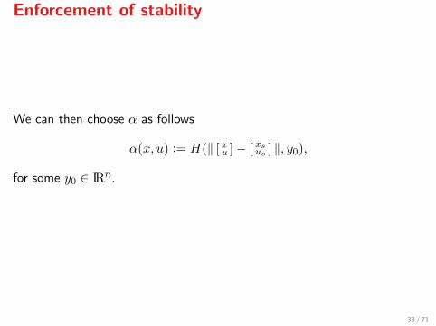
Enforcement of stability
We can then choose α as follows
α(x, u) := H(‖ [ xu ]− [ xsus ] ‖, y0),
for some y0 ∈ IRn.
33 / 71
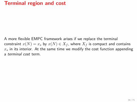
Terminal region and cost
A more flexible EMPC framework arises if we replace the terminalconstraint x(N) = xs by x(N) ∈ Xf , where Xf is compact and containsxs in its interior. At the same time we modify the cost function appendinga terminal cost term.
34 / 71
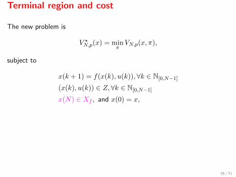
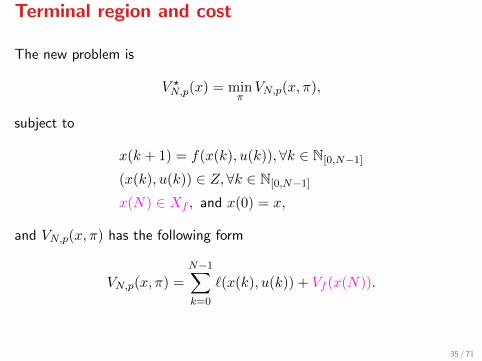
Terminal region and cost
The new problem is
V ?N,p(x) = min
πVN,p(x, π),
subject to
x(k + 1) = f(x(k), u(k)),∀k ∈ N[0,N−1]
(x(k), u(k)) ∈ Z, ∀k ∈ N[0,N−1]
x(N) ∈ Xf , and x(0) = x,
and VN,p(x, π) has the following form
VN,p(x, π) =
N−1∑k=0
`(x(k), u(k)) + Vf (x(N)).
35 / 71
Terminal region and cost
The new problem is
V ?N,p(x) = min
πVN,p(x, π),
subject to
x(k + 1) = f(x(k), u(k)),∀k ∈ N[0,N−1]
(x(k), u(k)) ∈ Z, ∀k ∈ N[0,N−1]
x(N) ∈ Xf , and x(0) = x,
and VN,p(x, π) has the following form
VN,p(x, π) =
N−1∑k=0
`(x(k), u(k)) + Vf (x(N)).
35 / 71
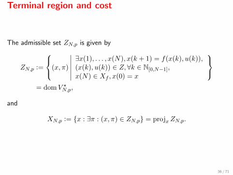
Terminal region and cost
The admissible set ZN,p is given by
ZN,p :=
(x, π)
∣∣∣∣∣∣∃x(1), . . . , x(N), x(k + 1) = f(x(k), u(k)),(x(k), u(k)) ∈ Z,∀k ∈ N[0,N−1],
x(N) ∈ Xf , x(0) = x
= domV ?
N,p,
and
XN,p := {x : ∃π : (x, π) ∈ ZN,p} = projx ZN,p.
36 / 71
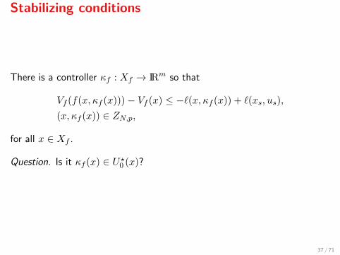
Stabilizing conditions
There is a controller κf : Xf → IRm so that
Vf (f(x, κf (x)))− Vf (x) ≤ −`(x, κf (x)) + `(xs, us),
(x, κf (x)) ∈ ZN,p,
for all x ∈ Xf .
Question. Is it κf (x) ∈ U?0 (x)?
37 / 71

Stability conditions
Theorem [Angeli et al. ’12] Under the above stabilizing conditions, if thesystem is strictly dissipative wrt s(x, u) = `(x, u)− `(xs, us), then xs is anasymptotically stable equilibrium point with domain of attraction XN,p.
Proof.For the proof we construct an equivalent optimisation problem defining
VN,p :=
N−1∑k=0
L(x(k), u(k)) + Vf (x(N)),
with Vf (x) := Vf (x) + λ(x)− λ(xs). Details: Angeli et al. ’12.
38 / 71

* Construction of Vf , κf and Xf
How can we cosntruct Vf , κf and Xf so that
Vf (f(x, κf (x)))− Vf (x) ≤ −`(x, κf (x)) + `(xs, us),
(x, κf (x)) ∈ ZN,p,
for all x ∈ Xf?
The answer is not trivial and there exist various approaches; see Amrit etal. 2011.
39 / 71
* Construction of Vf , κf and Xf
Assumption. Functions f and ` are twice continuously differentiable,f(0, 0) = 0 and xs = us = 0. The linearised system
x(k + 1) = Ax(k) +Bu(k),
with A = fx(0, 0) and B = fu(0, 0) is stabilisable, so there exists a lineargain K so that AK = A+BK is stable.
40 / 71
* Construction of Vf , κf and Xf
Define ¯(x) := `(x,Kx)− `(0, 0). Find Q? so that
x′(Q? − ¯xx(x))x ≥ 0,∀x ∈ X,
Define Q := Q? + αI, for some α > 0. Define q = ¯x(0). Choose P to be
the solution of the Lyapunov equation
A′KPAK − P = −Q.
Define p := q′(I −AK)−1. Take a ball Bδ ⊆ {x ∈ IRn : (x,Kx) ∈ Z}.Define Vf (x) := 1
2x′Px+ p′x. Take β > 0 so that Xf := lev≤β Vf ⊆ Bδ,
and κf (x) := Kx.
41 / 71
End of third section
Conclusions.
1. The rotated cost is equivalent to the original cost
2. Strict dissipativity entails as. stability
3. We may enforce stability by adding a PD function α(x, u) to thestage cost
4. We may replace x(N) = xs by x(N) ∈ Xf and then
5. To have as. stability we need to add a terminal cost Vf and draw anassumption about Vf over Xf
42 / 71
IV. Averagely constrained MPC

Asymptotic averaging operator
Take v ∈ `∞(IRnv), that is v = {v(i)}i∈N and there is a M ≥ 0 so that forall i ∈ N, ‖v(i)‖ ≤M . We define
Av[v] =
{v ∈ IRnv | ∃{tn}n∈N ⊆ N, s.t.
∑tnk=0 ν(k)
tn + 1
n−→ v
}.
43 / 71

Asymptotic averaging operator
Examples.
Take v = {0, 1, 0, 0, 1, 0, 0, 0, 1, . . .}. Then, verify that Av[v] = 0.
For v = {0, 1, 0, 0, 1, 1, 0, 0, 0, 0, 1, 1, 1, 1, . . . . . .}, we can verify thatAv[v] = [1/3, 1/2].
44 / 71

Asymptotic averaging operator
Properties.
For v ∈ `∞(IRnv) define the P -shifted variant of v as w = {w(j)}k∈N withw(j) = v(j + P ). Then, Av[v] = Av[w] and
Av ([ vw ]) ⊆ {[ v1v2 ] ∈ IR2nv : v1 = v2}.
45 / 71

Average constraints
Consider the system
x(k + 1) = f(x(k), u(k)),
y(k) = h(x(k), u(k)).
with h : Z → IRp. The following constraints are imposed:
Av[y] ∈ Y ,
where Y ⊆ IRp is closed, convex and contains h(xs, us).
46 / 71
EMPC with average constraints
Our goal is to design a receding horizon control strategy with:
X Recursive feasibility
X [Performance bounds] Av[`(x, u)] ⊆ (−∞, `(xs, us)],X [Constraints satisfaction] (x(k), u(k)) ∈ Z, for k ∈ N,
X [Asymptotic average constraints] Av[y] ∈ Y .
47 / 71
Averagely constrained EMPC
To this end, at time t we sove the problem:
V ?N,a(x; t) = min
π
N−1∑k=0
`(x(k), u(k)),
subject to the constraints:
x(k + 1) = f(x(k), u(k)),∀k ∈ N[0,N−1],
(x(k), u(k)) ∈ Z, ∀k ∈ N[0,N−1],
x(N) = xs, x(0) = x,
N−1∑k=0
h(x(k), u(k)) ∈ Yt.
where Yt is time-varying.
48 / 71
Averagely constrained EMPC
. . . where4
Yt+1 = Yt ⊕ Y {h(x(t), u(t))},
andY0 = NY + Y ,
where Y is any compact convex set containing the origin.
We’ll prove that: The resulting MPC controller is recursively feasible andall requirements are satisfied for the closed-loop system.
4C {z} := {y : y + z ∈ C}.49 / 71
Averagely constrained EMPC
Define
ZN,a(t) :=
(x, π)
∣∣∣∣∣∣∣∣∃x(1), . . . , x(N), x(k + 1) = f(x(k), u(k)),(x(k), u(k)) ∈ Z, ∀k ∈ N[0,N−1],
x(N) = xs, x(0) = x∑N−1k=0 h(x(k), u(k)) ∈ Yt
= domV ?
N (·, t),
and
XN,a(t) := {x : ∃π : (x, π) ∈ ZN,a(t)}= projx ZN,a(t).
The receding horizon controller is a mapping κN,a : IRn × N→ IRm suchthat (x, κN,a(x, t)) ∈ ZN,a(t) whenever x ∈ XN,a(t).
50 / 71
Recursive feasibility of AC-EMPC
The averagely constrained EMPC is recursively feasible: if x(t) ∈ XN,a(t),then x(t+ 1) ∈ XN,a(t+ 1).
Proof. Exercise. show that x(t+ 1) = f(x, κN,a(x, t)) ∈ XN,a(t+ 1)given that take x(t) = x ∈ XN,a(t).
51 / 71
Asymptotic average performance
The asymptotic average performance of AC-EMPC is no worse than thecost of best admissible steady state, that is
Av[`(x, u)] ⊆ (−∞, `(xs, us)]
Proof. Exercise. we need to prove that
lim supT→∞
∑T−1k=0 `(x(k), u(k))
T≤ `(xs, us).
Start by verifying that V ?N,a(x
+)− V ?N,a(x) ≤ `(xs, us)− `(x, u).
52 / 71
Average constraints satisfaction
Av[y] ⊆ Y .
Proof. The EMPC controller produces the following sequence of sets Yt:
Yt = Y ⊕ (t+N)Y {t−1∑k=0
y(k)}.
According to the problem constraints:
N−1∑k=0
h(x(k), u(k)) ∈ Yt
⇔N−1∑k=0
h(x(k), u(k)) +
t−1∑k=0
y(k) ∈ Y ⊕ (t+N)Y
53 / 71
Average constraints satisfaction
Proof (cont’d).Thus
N−1∑k=0
h(x(k), u(k)) ∈N−1⊕k=0
h(Z),
which is a compact set since Z is compact and h is continuous. Take{tn}n ⊆ N so that the limit limn
∑tnk=0 y(k)/tn exists; then
limn
tn∑k=0
y(k)
tn∈ lim
n
Y + (tn + 1 +N)Y
tn + 1= Y,
thus Av[y] ⊆ Y .
54 / 71

End of fourth section
Conclusions.
1. We introduced the asymptotic average operator Av[·]2. This allows us to impose constraints on the asymptotic average of the
output y
3. and the asymptotic average of the cost as well
4. We formulated an asymptotically constrained EMPC and
5. we showed that it is recursively feasible and satisfies the prescribed as.average constraints
55 / 71
V. Average performance
56 / 71
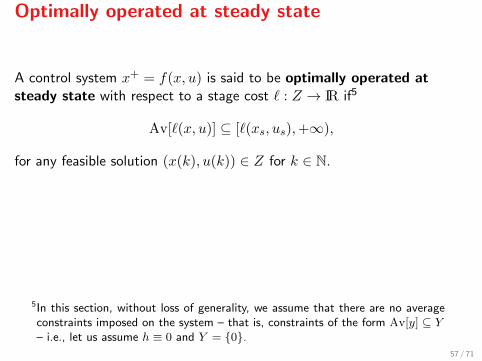
Optimally operated at steady state
A control system x+ = f(x, u) is said to be optimally operated atsteady state with respect to a stage cost ` : Z → IR if5
Av[`(x, u)] ⊆ [`(xs, us),+∞),
for any feasible solution (x(k), u(k)) ∈ Z for k ∈ N.
Equivalently:
lim infT→∞
∑T−1k=0 `(x(k), u(k))
T≥ `(xs, us).
5In this section, without loss of generality, we assume that there are no averageconstraints imposed on the system – that is, constraints of the form Av[y] ⊆ Y– i.e., let us assume h ≡ 0 and Y = {0}.
57 / 71
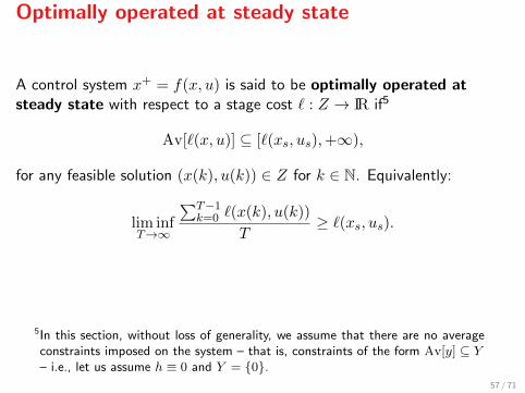
Optimally operated at steady state
A control system x+ = f(x, u) is said to be optimally operated atsteady state with respect to a stage cost ` : Z → IR if5
Av[`(x, u)] ⊆ [`(xs, us),+∞),
for any feasible solution (x(k), u(k)) ∈ Z for k ∈ N. Equivalently:
lim infT→∞
∑T−1k=0 `(x(k), u(k))
T≥ `(xs, us).
5In this section, without loss of generality, we assume that there are no averageconstraints imposed on the system – that is, constraints of the form Av[y] ⊆ Y– i.e., let us assume h ≡ 0 and Y = {0}.
57 / 71
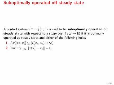
Suboptimally operated off steady state
A control system x+ = f(x, u) is said to be suboptimally operated offsteady state with respect to a stage cost ` : Z → IR if it is optimallyoperated at steady state and either of the following holds
1. Av[`(x, u)] ⊆ (`(xs, us),+∞),
2. lim infk→∞ ‖x(k)− xs‖ = 0.
58 / 71
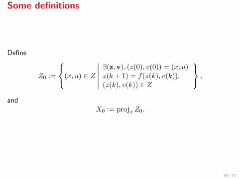
Some definitions
Define
Z0 :=
(x, u) ∈ Z
∣∣∣∣∣∣∃(z,v), (z(0), v(0)) = (x, u)z(k + 1) = f(z(k), v(k)),(z(k), v(k)) ∈ Z
,
andX0 := projx Z0.
59 / 71

Available storage function
For x ∈ X0, we define the available storage function with respect to asupply rate s : Z → IR as follows
S(x) := supT≥0z(0)=x
z(k+1)=f(z(k),v(k)),k∈N(z(k),v(k))∈Z,k∈N
T−1∑k=0
−s(z(k), v(k))
Remark: S(x) ≥ 0, for all x ∈ X.
60 / 71
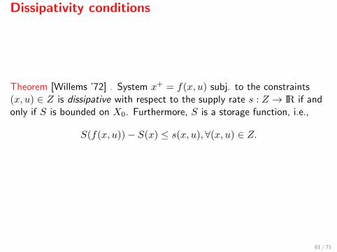
Dissipativity conditions
Theorem [Willems ’72] . System x+ = f(x, u) subj. to the constraints(x, u) ∈ Z is dissipative with respect to the supply rate s : Z → IR if andonly if S is bounded on X0. Furthermore, S is a storage function, i.e.,
S(f(x, u))− S(x) ≤ s(x, u), ∀(x, u) ∈ Z.
61 / 71
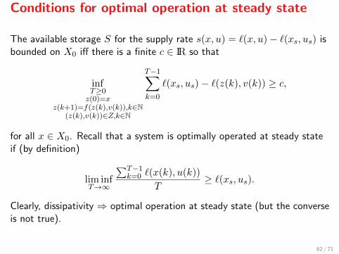
Conditions for optimal operation at steady state
The available storage S for the supply rate s(x, u) = `(x, u)− `(xs, us) isbounded on X0 iff there is a finite c ∈ IR so that
infT≥0z(0)=x
z(k+1)=f(z(k),v(k)),k∈N(z(k),v(k))∈Z,k∈N
T−1∑k=0
`(xs, us)− `(z(k), v(k)) ≥ c,
for all x ∈ X0. Recall that a system is optimally operated at steady stateif (by definition)
lim infT→∞
∑T−1k=0 `(x(k), u(k))
T≥ `(xs, us).
Clearly, dissipativity ⇒ optimal operation at steady state (but the converseis not true).
62 / 71
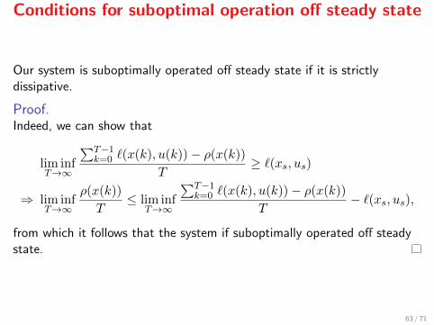
Conditions for suboptimal operation off steady state
Our system is suboptimally operated off steady state if it is strictlydissipative.
Proof.Indeed, we can show that
lim infT→∞
∑T−1k=0 `(x(k), u(k))− ρ(x(k))
T≥ `(xs, us)
⇒ lim infT→∞
ρ(x(k))
T≤ lim inf
T→∞
∑T−1k=0 `(x(k), u(k))− ρ(x(k))
T− `(xs, us),
from which it follows that the system if suboptimally operated off steadystate.
63 / 71
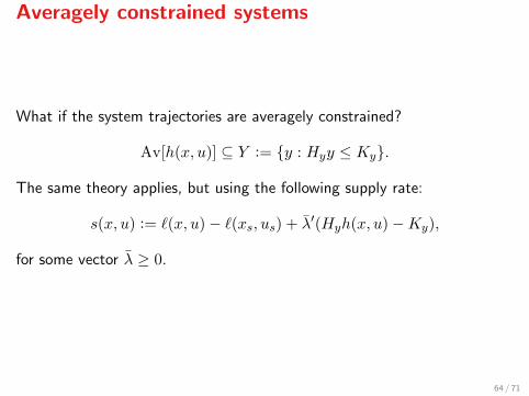
Averagely constrained systems
What if the system trajectories are averagely constrained?
Av[h(x, u)] ⊆ Y := {y : Hyy ≤ Ky}.
The same theory applies, but using the following supply rate:
s(x, u) := `(x, u)− `(xs, us) + λ′(Hyh(x, u)−Ky),
for some vector λ ≥ 0.
64 / 71
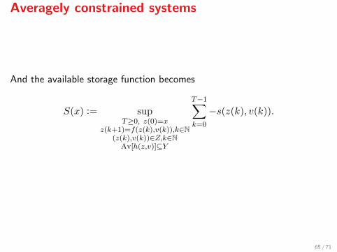
Averagely constrained systems
And the available storage function becomes
S(x) := supT≥0, z(0)=x
z(k+1)=f(z(k),v(k)),k∈N(z(k),v(k))∈Z,k∈N
Av[h(z,v)]⊆Y
T−1∑k=0
−s(z(k), v(k)).
65 / 71
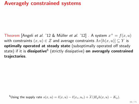
Averagely constrained systems
Theorem [Angeli et al. ’12 & Muller et al. ’12] . A system x+ = f(x, u)with constraints (x, u) ∈ Z and average constraints Av[h(x, u)] ⊆ Y isoptimally operated at steady state (suboptimally operated off steadystate) if it is dissipative6 (strictly dissipative) on averagely constrainedtrajectories.
6Using the supply rate s(x, u) = `(x, u)− `(xs, us) + λ′(Hyh(x, u)−Ky).
66 / 71
End of fifth section
Conclusions.
1. We introduced the notions of optimal operation at steady state andsuboptimal operation off steady state
2. We elaborated on the powerful notion of available storage and
3. presented Willem’s dissipativity theorem
4. We used the available storage function to determine conditions forOOSS and SOOSS
67 / 71
VI. Conclusions
Conclusions
1. EMPC combines process economics and control in a natural way
2. Stability not for granted
3. Dissipativity plays a crucial role in proving stability and optimaloperation at steady state
4. Standard MPC practices can still be used
68 / 71

Extensions
1. EMPC without a terminal constraint (Grune, 2013)
2. Generalized terminal state constraint: unifying tracking and economicMPC (Fagiano and Teel, 2013)
3. A Lyapunov function for EMPC (Diehl et al., 2011)
4. Scenario-based EMPC (Bø and Johansen, 2014)
69 / 71
Topics for research
1. Robust EMPC: how resilient is EMPC to disturbances and how maydisturbances affect average performance?
2. EMPC for uncertain systems in presence of probabilistic information(e.g., Markovian switching systems)
3. Lyapunov theorems for averagely constrained EMPC
4. Applications of EMPC
70 / 71
References
1. J.B. Rawlings, D. Angeli and C.N. Bates, Fundamentals of economic modelpredictive control, 51st IEEE conf. Dec. and Contr., Hawaii, Maui, USA, 2012.
2. D. Angeli, R. Amrit and J.B. Rawlings, On average performance and stability ofeconomic model predictive control, IEEE Trans. Aut. Contr. 57(7), 2012.
3. L. Fagiano and A.R. Teel, Generalized terminal state constraint for modelpredictive control, Automatica 49, 2013.
4. L. Grune, Economic receding horizon control without terminal constraints,Automatica 49, 2013.
5. M. Diehl, R. Amrit and J.B. Rawlings, A Lyapunov function for economicoptimizing model predictive control, IEEE Trans. Aut. Contr 56(3), 2011.
6. J.C. Willems, Dissipative dynamical systems – part I: General theory, Archive forrational mechanics and analysis 45(5), pp. 321-351, 1972.
7. M.A. Muller, D. Angeli and F. Allgower, On convergence of averagely constrainedeconomic MPC and necessity of dissipativity for optimal steady-state operation, In:American Control Conference (ACC), Washington, 2013.
8. M.A. Muller, D. Angeli and F. Allgower, Economic model predictive control withself-tuning terminal cost, European Journal of Control 19, pp. 408-416, 2013.
71 / 71