economic growth: the neo-classical & endogenous...
TRANSCRIPT

Historical Growth Patterns Assumptions & Setup Solow Growth Model Solow with Technology TFP Exercise Endogenous Multiple
Economic Growth: The Neo-classical &
Endogenous Story
EC307 ECONOMIC DEVELOPMENT
Dr. Kumar Aniket
University of Cambridge & LSE Summer School
Lecture 4
created on June 6, 2010
c©Kumar Aniket

Historical Growth Patterns Assumptions & Setup Solow Growth Model Solow with Technology TFP Exercise Endogenous Multiple
Density of countries
1960
19802000
0 20,000 40,000 60,000GDP per capita ($)
FIGURE 1.1 Estimates of the distribution of countries according to PPP-adjusted GDP per capita in1960, 1980, and 2000.
c©Kumar Aniket

Historical Growth Patterns Assumptions & Setup Solow Growth Model Solow with Technology TFP Exercise Endogenous Multiple
Density of countries
1960
1980
2000
6 8 10 12Log GDP per capita
FIGURE 1.2 Estimates of the distribution of countries according to log GDP per capita (PPP adjusted)in 1960, 1980, and 2000.
c©Kumar Aniket
Historical Growth Patterns Assumptions & Setup Solow Growth Model Solow with Technology TFP Exercise Endogenous Multiple
Density of countries (weighted by population)
1960
19802000
6 8 10 12Log GDP per capita
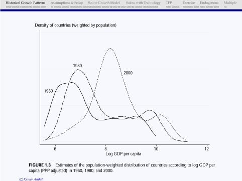
FIGURE 1.3 Estimates of the population-weighted distribution of countries according to log GDP percapita (PPP adjusted) in 1960, 1980, and 2000.
c©Kumar Aniket

Historical Growth Patterns Assumptions & Setup Solow Growth Model Solow with Technology TFP Exercise Endogenous Multiple
Density of countries
1960
1980
2000
6 8 10 12Log GDP per worker
FIGURE1.4 Estimates of the distribution of countries according to log GDP per worker (PPP adjusted)in 1960, 1980, and 2000.
c©Kumar Aniket

Historical Growth Patterns Assumptions & Setup Solow Growth Model Solow with Technology TFP Exercise Endogenous Multiple
Log consumption per capita, 2000
15
14
13
12
11
10
AFG
ALB
DZA
AGO
ATG
ARG
ARM
AUSAUT
AZE
BHS
BHR
BGD
BRB
BLR
BEL
BLZ
BEN
BMU
BTN
BOLBIH
BWA
BRABRN
BGR
BFA
BDI
KHM
CMR
CAN
CPV
CAF
TCD
CHL
CHN
COL
COM
ZAR
COG
CRI
CIV
HRV
CUB
CYP
CZE
DNK
DJI DMA
DOM
ECU
EGYSLV
GNQ
ERI
EST
ETH
FJI
FIN
FRA
GAB
GMB
GEO
GER
GHA
GRC
GRD
GTM
GIN
GNB
GUYHTIHND
HKG
HUN
ISL
IND
IDN
IRN
IRQ
IRLISRITA
JAM
JPN
JOR
KAZ
KEN
KIR
PRK
KOR
KWT
KGZ
LAO
LVALBN
LSO
LBR
LBYLTU
LUX
MAC
MKD
MDGMWI
MYS
MDV
MLI
MLT
MRT
MUS
MEX
FSMMDA
MNG
MAR
MOZ
NAM
NPL
NLD
ANT
NZL
NIC
NER NGA
NOR
OMN
PAK
PLWPAN
PNG
PRY
PERPHL
POL
PRTPRI
QAT
ROM RUS
RWA
WSM
STP
SAU
SENSCG
SYC
SLE
SGP
SVK
SVN
SLB
SOM
ZAF
ESP
LKA
KNA
LCA
VCT
SDN
SUR
SWZ
SWE
CHE
SYR
TWN
TJK
TZA
THA
TGO
TON
TTO
TUN
TUR
TKM
UGA
UKR
AREGBR
USA
URY
UZBVUT
VEN
VNM
YEM
ZMB
ZWE
6 7 8 9 10 11Log GDP per capita, 2000
FIGURE 1.5 The association between income per capita and consumption per capita in 2000. For adefinition of the abbreviations used in this and similar figures in the book, see http://unstats.un.org/unsd/methods/m49/m49alpha.htm.
c©Kumar Aniket

Historical Growth Patterns Assumptions & Setup Solow Growth Model Solow with Technology TFP Exercise Endogenous Multiple
Life expectancy, 2000 (years)
AFG
AGO
ALB
ANT
ARE
ARG
ARM
AUSAUT
AZE
BDI
BEL
BEN
BFA
BGD
BGR
BHR
BHS
BIH
BLR
BLZ
BOL
BRA
BRB
BRN
BTN
BWA
CAF
CANCHE
CHL
CHN
CIVCMR
COG
COL
COM
CPV
CRICUBCYP
CZE
DJI
DNK
DOM
DZAECU
EGY
ERI
ESP
EST
FIN
FJI
FRA
FSM
GAB
GBR
GEO
GHA
GINGMB
GNBGNQ
GRC
GTM
GUY
HKG
HND
HRV
HTI
HUN
IDN
IND
IRL
IRN
IRQ
ISLISRITA
JAMJOR
JPN
KAZ
KEN
KGZ
KHM
KOR
KWT
LAO
LBN
LBR
LBYLCALKA
LSO
LTU
LUX
LVA
MAC
MAR
MDA
MDG
MDV
MEXMKD
MLI
MLT
MNG
MOZ
MRT
MUS
MWI
MYS
NAM
NERNGA
NIC
NLD NOR
NPL
NZL
OMN
PAK
PAN
PERPHL
PNG
POLPRI
PRK
PRT
PRY
QAT
ROM
RUS
RWA
SAUSCG
SDN SEN
SGP
SLB
SLE
SLV
SOM
STP
SUR
SVK
SVN
SWE
SWZ
SYR
TCD
TGO
THA
TJKTKM
TON
TTO
TUN
TUR
TZA
UGA
UKR
URY
USA
UZB
VCTVEN
VNMVUTWSM
YEMZAF
ZMB
ZWE
ETH
GER
30
40
50
60
70
80
6 7 8 9 10 11Log GDP per capita, 2000
FIGURE 1.6 The association between income per capita and life expectancy at birth in 2000.c©Kumar Aniket
Historical Growth Patterns Assumptions & Setup Solow Growth Model Solow with Technology TFP Exercise Endogenous Multiple
Density of countries
19601980
2000
–0.1 0.0 0.1 0.2Average growth rate of GDP per worker
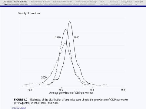
FIGURE 1.7 Estimates of the distribution of countries according to the growth rate of GDP per worker(PPP adjusted) in 1960, 1980, and 2000.
c©Kumar Aniket

Historical Growth Patterns Assumptions & Setup Solow Growth Model Solow with Technology TFP Exercise Endogenous Multiple
Log GDP per capita
United States
UnitedKingdom
Spain
SingaporeBrazil
South Korea
Botswana
Guatemala
Nigeria
India
7
8
9
10
11
1960 1970 1980 1990 2000
FIGURE 1.8 The evolution of income per capita in the United States, the United Kingdom, Spain,Singapore, Brazil, Guatemala, South Korea, Botswana, Nigeria, and India, 1960–2000.c©Kumar Aniket
Historical Growth Patterns Assumptions & Setup Solow Growth Model Solow with Technology TFP Exercise Endogenous Multiple
Log GDP per worker relative to the United States, 2000
1.1
1.0
0.9
0.8
0.7
0.6
DZA
ARG
AUSAUT
BRB
BEL
BEN
BOL
BRA
BFA
BDI
CMR
CAN
CPV
TCD
CHL
CHN
COL
COMCOG
CRI
CIV
DNK
DOM
ECUEGY SLV
GNQ
ETH
FINFRA
GAB
GMB
GHA
GRC
GTM
GIN
GNB
HND
HKGISL
IND
IDN
IRN
IRLISRITA
JAM
JPN
JOR
KEN
KOR
LSO
LUX
MDGMWI
MYS
MLI
MUS
MEX
MAR
MOZ
NPL
NLD
NZL
NIC
NER
NGA
NOR
PAK
PAN
PRYPER
PHL
PRT
ROM
RWA
SEN
SGP
ZAF
ESP
LKA
SWECHE
SYR
TZA
THA
TGO
TTO
TUR
UGA
GBR
USA
URY
VEN
ZMB
ZWE
0.6 0.7 0.8 0.9 1.0 1.1Log GDP per worker relative to the United States, 1960
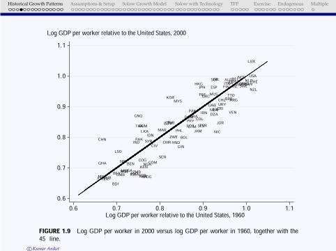
FIGURE 1.9 Log GDP per worker in 2000 versus log GDP per worker in 1960, together with the45� line.
c©Kumar Aniket

Historical Growth Patterns Assumptions & Setup Solow Growth Model Solow with Technology TFP Exercise Endogenous Multiple
Log GDP per capita
Western offshoots
Western Europe
Africa
Asia
Latin America
6
7
8
9
10
1820 1850 1900 1950 2000
FIGURE 1.10 The evolution of average GDP per capita in Western offshoots, Western Europe, LatinAmerica, Asia, and Africa, 1820–2000.
c©Kumar Aniket

Historical Growth Patterns Assumptions & Setup Solow Growth Model Solow with Technology TFP Exercise Endogenous Multiple
Log GDP per capita
Western offshoots
Western Europe
Africa
Asia
LatinAmerica
6
7
8
9
10
1000 1200 1400 1600 1800 2000
FIGURE 1.11 The evolution of average GDP per capita in Western offshoots, Western Europe, LatinAmerica, Asia, and Africa, 1000–2000.
c©Kumar Aniket

Historical Growth Patterns Assumptions & Setup Solow Growth Model Solow with Technology TFP Exercise Endogenous Multiple
Log GDP per capita
United Kingdom
United States
Spain
China
Brazil
India
Ghana
6
7
8
9
10
1820 1850 1900 1950 2000
FIGURE 1.12 The evolution of income per capita in the United States, the United Kindgom, Spain,Brazil, China, India, and Ghana, 1820–2000.
c©Kumar Aniket

Historical Growth Patterns Assumptions & Setup Solow Growth Model Solow with Technology TFP Exercise Endogenous Multiple
Average growth rate of GDP, 1960–2000
0.06
0.04
0.02
0.00
–0.02
TWN
CHN GNQKOR
HKGTHA MYS
ROM JPN SGPIRL
LKA LUXGHA LSO
PAKPRT ESP
AUTIND GRC
IDN CPV MUS ISRBELEGY ITATUR FRA
MAR FIN NORPANSYRDOM GBR
MWI NPL BRAISL
DNK USAGAB NLD
TZA CIV PHLPRY IRN CHL TTO SWECAN
CHE
ETH AUSGNB
BFA BEN COL MEX BRBZWE ECU ZAFURY
GMB COG CRI ARGMLI CMR GTMMOZUGA DZA NZL
HND BOL SLVBDI
ZMB NGA PERTGO KEN JAMRWA COM SEN
GIN VENTCD JORNER
MDGNIC
7 8 9 10 11Log GDP per worker, 1960
FIGURE 1.13 Annual growth rate of GDP per worker between 1960 and 2000 versus log GDP perworker in 1960 for the entire world.
c©Kumar Aniket
Historical Growth Patterns Assumptions & Setup Solow Growth Model Solow with Technology TFP Exercise Endogenous Multiple
Average growth rate of GDP, 1960–2000
AUS
BEL
CAN
DNK
FIN
FRA
GRC
ISL
IRL
ITA
JPN
LUX
NLD
NOR
PRT ESP
SWE
CHE
TUR
GBRUSA
0.01
0.02
0.03
0.04
8.5 9.0 9.5 10. 0 10. 5Log GDP per worker, 1960
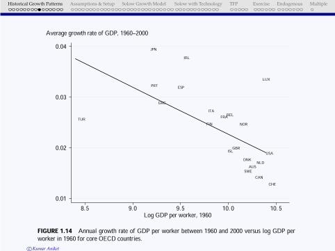
FIGURE 1.14 Annual growth rate of GDP per worker between 1960 and 2000 versus log GDP perworker in 1960 for core OECD countries.
c©Kumar Aniket

Historical Growth Patterns Assumptions & Setup Solow Growth Model Solow with Technology TFP Exercise Endogenous Multiple
Average growth rate of GDP per capita, 1960–2000
ARG
AUS
AUTBEL
BENBOL
BRA
BFA
CANCHL
CHN
COLCRI
DNK
DOM
ECU
EGY
SLV
ETH
FINFRAGHA
GRC
GTM
GIN
HND
ISLIND
IRN
IRL
ISRITA
JAM
JPN
JOR
KEN
KOR
LUX
MWI
MYS
MUS
MEX
MAR NLD
NZL
NIC
NGA
NOR
PAK
PAN
PRY
PER
PHL
PRT
ZAF
ESPLKA
SWE
CHE
TWN
THA
TTOTUR
UGA
GBRUSA
URY
VENZMB
ZWE
0.00
0.02
0.04
0.06
0.08
0.0 0.1 0.2 0.3 0.4Average investment rate, 1960–2000
FIGURE 1.15 The relationship between average growth of GDP per capita and average growth ofinvestments to GDP ratio, 1960–2000.
c©Kumar Aniket

Historical Growth Patterns Assumptions & Setup Solow Growth Model Solow with Technology TFP Exercise Endogenous Multiple
Average growth rate of GDP per capita, 1960–2000
0.06
0.04
0.02
0.00
–0.02
TWN
CHN
RWA
KOR
HKGTHAMYS
SGP IRLJPN
LKA
EGY IDNPAK GHA LSO
IND
PRT
SYRTUN TUR MUS
ESP
ITA
PANFRA
GRCAUT
BELFIN NORISR
BDI
BENMLIGMBMOZ
NPL
SLV BOL PER
MWI BRA
CMR ZAFCOG
ZWE COL MEXECU
UGADZA CRI
DOM
GTM
HND
IRN
TGO KEN ZMBJAM
PRY
ARG
CHL
ISL
PHLTTOURY BRB
NLDGBR
AUSCAN
CHE
DNKSWE
NZL
USA
SENVEN
JORNER
NIC
0 2 4 6 8 10 12Average years of schooling, 1960–2000
FIGURE 1.16 The relationship between average growth of GDP per capita and average years ofschooling, 1960–2000.
c©Kumar Aniket

Historical Growth Patterns Assumptions & Setup Solow Growth Model Solow with Technology TFP Exercise Endogenous Multiple
Density of countries (weighted by population)
1960
19802000
6 8 10 12Log GDP per capita
FIGURE 1.3 Estimates of the population-weighted distribution of countries according to log GDP percapita (PPP adjusted) in 1960, 1980, and 2000.
c©Kumar Aniket

Historical Growth Patterns Assumptions & Setup Solow Growth Model Solow with Technology TFP Exercise Endogenous Multiple
Density of countries
1960
1980
2000
6 8 10 12Log GDP per worker
FIGURE1.4 Estimates of the distribution of countries according to log GDP per worker (PPP adjusted)in 1960, 1980, and 2000.
c©Kumar Aniket

Historical Growth Patterns Assumptions & Setup Solow Growth Model Solow with Technology TFP Exercise Endogenous Multiple
Log consumption per capita, 2000
15
14
13
12
11
10
AFG
ALB
DZA
AGO
ATG
ARG
ARM
AUSAUT
AZE
BHS
BHR
BGD
BRB
BLR
BEL
BLZ
BEN
BMU
BTN
BOLBIH
BWA
BRABRN
BGR
BFA
BDI
KHM
CMR
CAN
CPV
CAF
TCD
CHL
CHN
COL
COM
ZAR
COG
CRI
CIV
HRV
CUB
CYP
CZE
DNK
DJI DMA
DOM
ECU
EGYSLV
GNQ
ERI
EST
ETH
FJI
FIN
FRA
GAB
GMB
GEO
GER
GHA
GRC
GRD
GTM
GIN
GNB
GUYHTIHND
HKG
HUN
ISL
IND
IDN
IRN
IRQ
IRLISRITA
JAM
JPN
JOR
KAZ
KEN
KIR
PRK
KOR
KWT
KGZ
LAO
LVALBN
LSO
LBR
LBYLTU
LUX
MAC
MKD
MDGMWI
MYS
MDV
MLI
MLT
MRT
MUS
MEX
FSMMDA
MNG
MAR
MOZ
NAM
NPL
NLD
ANT
NZL
NIC
NER NGA
NOR
OMN
PAK
PLWPAN
PNG
PRY
PERPHL
POL
PRTPRI
QAT
ROM RUS
RWA
WSM
STP
SAU
SENSCG
SYC
SLE
SGP
SVK
SVN
SLB
SOM
ZAF
ESP
LKA
KNA
LCA
VCT
SDN
SUR
SWZ
SWE
CHE
SYR
TWN
TJK
TZA
THA
TGO
TON
TTO
TUN
TUR
TKM
UGA
UKR
AREGBR
USA
URY
UZBVUT
VEN
VNM
YEM
ZMB
ZWE
6 7 8 9 10 11Log GDP per capita, 2000
FIGURE 1.5 The association between income per capita and consumption per capita in 2000. For adefinition of the abbreviations used in this and similar figures in the book, see http://unstats.un.org/unsd/methods/m49/m49alpha.htm.
c©Kumar Aniket

Historical Growth Patterns Assumptions & Setup Solow Growth Model Solow with Technology TFP Exercise Endogenous Multiple
Output
•k(t)
f(k(t))
f (k*)
Consumptionsf (k(t ))
sf(k*)
Investment
0 k*k(t )
FIGURE 2.4 Investment and consumption in the steady-state equilibrium.
c©Kumar Aniket

Historical Growth Patterns Assumptions & Setup Solow Growth Model Solow with Technology TFP Exercise Endogenous Multiple
LONG-RUN GROWTH:
Point of Departure from the short run IS-LM analysis you have may
have done. . .
Ignore the Demand Side
• Assumption: Prices are flexible
• Assumption: Agents form correct expectations
Carefully specify the supply side
L Labour is exogenously given
K Capital is endogenous over time
A Technology exogenous to start with . . .
c©Kumar Aniket

Historical Growth Patterns Assumptions & Setup Solow Growth Model Solow with Technology TFP Exercise Endogenous Multiple
THE PRODUCTION FUNCTION
Y = F(K,L) where Y = output
K = capital (input / factor)
L = labour (input / factor)
Assumptions:
• Constant Returns to Scale: scale up or scale down the economy – on
worker firm can gives us the intuition of the economy
• Marginal Products positive and diminishing: factors are productive,
but at a decreasing rate.
c©Kumar Aniket

Historical Growth Patterns Assumptions & Setup Solow Growth Model Solow with Technology TFP Exercise Endogenous Multiple
MARGINAL PRODUCTS
Marginal Product of Labour:
∂Y
∂L= FL > 0 positive
∂ 2Y
∂L2= FLL < 0 and diminishing
• labour contributes positively to the output but each subsequent
contribution is smaller.
Marginal Product of Capital:
∂Y
∂K= FK > 0 positive
∂ 2Y
∂K2= FKK < 0 and diminishing
• capital contributes positively to the output but each subsequent
contribution is smaller.c©Kumar Aniket

Historical Growth Patterns Assumptions & Setup Solow Growth Model Solow with Technology TFP Exercise Endogenous Multiple
Constant Return to Scale → Representative Firm
Size does not matter
• The whole country could be one firm
• Alternative, the country could be divided into infinite number of
tiny firms
We try to understand the economy by understanding the action
of a single representative firm
c©Kumar Aniket

Historical Growth Patterns Assumptions & Setup Solow Growth Model Solow with Technology TFP Exercise Endogenous Multiple
COBB-DOUGLAS PRODUCTION FUNCTION
Y = Kα(AL)1−α
A: constant (represents state of technology)
A plays a key role in theory of growth
check whether Cobb-Douglas Production function . . .
• exhibits constant returns of scale?
• has complementarity of factors?
• satisfies the Euler’s theorem?
c©Kumar Aniket

Historical Growth Patterns Assumptions & Setup Solow Growth Model Solow with Technology TFP Exercise Endogenous Multiple
A
O k
f(k)
y
k0 k
1k
2k
3k
4
y*
B
C
DE F
y0
k5
Figure: Per worker production function
c©Kumar Aniket
Historical Growth Patterns Assumptions & Setup Solow Growth Model Solow with Technology TFP Exercise Endogenous Multiple
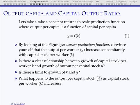
OUTPUT CAPITA AND CAPITAL OUTPUT RATIO
Lets take a take a constant returns to scale production function
where output per capita is a function of capital per capita
y = f (k) (1)
By looking at the Figure per worker production function, convince
yourself that the output per worker (y) increase concomitantly
with capital stock per worker (k)
Is there a clear relationship between growth of capital stock per
worker k and growth of output per capital stock y?
Is there a limit to growth of k and y?
What happens to the output per capital stock( y
k
)as capital stock
per worker (k) increases?
c©Kumar Aniket

Historical Growth Patterns Assumptions & Setup Solow Growth Model Solow with Technology TFP Exercise Endogenous Multiple
If we can understand the growth dynamics for the above production
function, we can easily use different kinds of production functions to
understand the growth process of the economy. E.g.
Y = AKα L1−α
Y = (AK)α A1−α
We can even add other factors of production like H, human capital.
Y = AKα Hβ (L)1−α−β
c©Kumar Aniket

Historical Growth Patterns Assumptions & Setup Solow Growth Model Solow with Technology TFP Exercise Endogenous Multiple
A
B
CD O
E
k
y = f(k)
y
Figure: Constant Returns to Scale Production Function
c©Kumar Aniket

Historical Growth Patterns Assumptions & Setup Solow Growth Model Solow with Technology TFP Exercise Endogenous Multiple
FACTS OF GROWTH: THE KALDOR FACTS
KL grows at constant rate
r is constantYK is constant
w grows at a constant rate
Growth rate & Income levels vary substantially across countries
Growth rate not necessarily constant over time
c©Kumar Aniket
Historical Growth Patterns Assumptions & Setup Solow Growth Model Solow with Technology TFP Exercise Endogenous Multiple
BEHAVIOURAL FUNCTIONS
Saving: people save a constant (s) proportion of their income
S = s ·Y
Consumption: people consume (1− s) proportion of their income
C = (1− s) ·Y
Investment: all the saving in the economy gets invested
S = I
c©Kumar Aniket

Historical Growth Patterns Assumptions & Setup Solow Growth Model Solow with Technology TFP Exercise Endogenous Multiple
DEPRECIATION
Depreciation: Capital replaced due to wear and tear. machinery
needs to be serviced in order to be brought back to its original condition
• Capital depreciates at the rate of δCapital Formation: Any addition to capital stock first gets absorbed
by depreciation and the residual gets added to capital stock.
c©Kumar Aniket

Historical Growth Patterns Assumptions & Setup Solow Growth Model Solow with Technology TFP Exercise Endogenous Multiple
TWO KINDS OF INVESTMENT
Replacement Investment: compensates for depreciation
δK amount of capital depreciates & has to be replaced every
period
Net Investment: brand new capital stock or new machinery
added to the economy in a period
c©Kumar Aniket

Historical Growth Patterns Assumptions & Setup Solow Growth Model Solow with Technology TFP Exercise Endogenous Multiple
CAPITAL FORMATION
• Today’s investment is tomorrow’s capital
I = Kt+1 −Kt + δKt
= ∆Kt + δKt
Investment compensation for depreciation: δKt
today is addition to capital Stock: ∆Kt = Kt+1 −Kt
c©Kumar Aniket

Historical Growth Patterns Assumptions & Setup Solow Growth Model Solow with Technology TFP Exercise Endogenous Multiple
THE FUNDAMENTAL EQUATION
Saving Investment Equality
S = I
sY = ∆Kt +δKt
Fundamental equation:
∆kt
kt= s
[yt
kt
]
−δ
c©Kumar Aniket

Historical Growth Patterns Assumptions & Setup Solow Growth Model Solow with Technology TFP Exercise Endogenous Multiple
A
B
O k
f(k)
y
k0 k
1k
2k
3k
4 k*
y*
45°
B C
D
E F
G
H
s f (k)
δk
y0
c©Kumar Aniket
Historical Growth Patterns Assumptions & Setup Solow Growth Model Solow with Technology TFP Exercise Endogenous Multiple
In the Figure: Growth of capital per capita, start from an arbitrary
capital stock per worker k0 and find the net increase in k per
period
Illustrate how capital stock per worker increases from k0 to k∗ and
output per worker increases from y0 to y∗.
Why does capital stock per worker not increase beyond k∗?
Do you notice a pattern in the rate at which capital stock per
worker (k) and output per worker (y) grows?
Draw yourself another diagram and show what would happen if
we start from a situation where capital stock per worker of the
economy is greater than k∗ to start with. per worker (k) grows?
c©Kumar Aniket

Historical Growth Patterns Assumptions & Setup Solow Growth Model Solow with Technology TFP Exercise Endogenous Multiple
THE SOLOW MODEL
Definition (Solow Model I)
The most basic Solow model with no population growth or technological
progress.
Assumption
a) no population growth ⇒ ∆LL = 0
b) no technological progress ⇒ ∆AA = 0
c©Kumar Aniket

Historical Growth Patterns Assumptions & Setup Solow Growth Model Solow with Technology TFP Exercise Endogenous Multiple
FUNDAMENTAL EQUATION - I
Definition (Fundamental Equation - I)
∆Kt = s ·Yt −δ ·Kt
the part of savings that does not get absorbed by depreciation gets added
to capital stock
⊙ the fundamental equation
◦ derived from the saving investment equality
◦ would change to account for population growth
◦ would change to account for technological progress
c©Kumar Aniket

Historical Growth Patterns Assumptions & Setup Solow Growth Model Solow with Technology TFP Exercise Endogenous Multiple
GROWTH RATE OF CAPITAL STOCK
∆Kt = sY−δKt
∆Kt
Kt= s
Yt
Kt−δ
⊙ growth rate of capital
◦ increases with the saving rate s
◦ decrease with rate of depreciation δ◦ increases with output-capital ratio Yt
Kt
◦ YtKt
decreases as Kt increases
c©Kumar Aniket

Historical Growth Patterns Assumptions & Setup Solow Growth Model Solow with Technology TFP Exercise Endogenous Multiple
STEADY STATE
Definition (Steady State)
The economy reaches the steady state when the endogenous variable stop
changing
In Solow Model - I
◦ Endogenous variable: Kt
◦ Steady State Condition: ∆KtKt
= 0
∆Kt
Kt= s
Yt
Kt−δ = 0
⇒[
Y∗t
K∗t
]
=δs
c©Kumar Aniket

Historical Growth Patterns Assumptions & Setup Solow Growth Model Solow with Technology TFP Exercise Endogenous Multiple
GROWTH IN STEADY STATE
⊙ In Steady State[
Y∗t
K∗t
]
=δs
◦ output-capital ratio is constant
◦ Capital stops growing
◦ Output Stops growing
◦ No growth in steady state
⊙ Does this match our observation of the world?
c©Kumar Aniket
Historical Growth Patterns Assumptions & Setup Solow Growth Model Solow with Technology TFP Exercise Endogenous Multiple
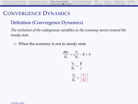
CONVERGENCE DYNAMICS
Definition (Convergence Dynamics)
The evolution of the endogenous variables as the economy moves toward the
steady state
⊙ When the economy is not in steady state
∆Kt
Kt= s
Yt
Kt−δ > 0
Yt
Kt>
δs
Yt
Kt>
[Y∗
t
K∗t
]
c©Kumar Aniket

Historical Growth Patterns Assumptions & Setup Solow Growth Model Solow with Technology TFP Exercise Endogenous Multiple
CONVERGENCE DYNAMICS
∆Kt
Kt= s
Yt
Kt−δ = s
(Yt
Kt−
[Y∗
t
K∗t
])
Assume: Kt < K∗t
◦ as Kt ↑ , capital-output ratio ↓◦ growth rate of capital is the difference between current
capital-output ratio and steady state capital-output ratio
◦ the further away from steady state the economy is, the faster the
rate at which capital grows
◦ the further away from steady state the economy is, the faster the
rate at which output grows
c©Kumar Aniket
Historical Growth Patterns Assumptions & Setup Solow Growth Model Solow with Technology TFP Exercise Endogenous Multiple
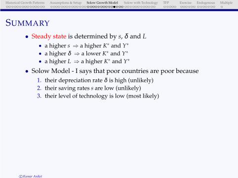
SUMMARY
• Steady state is determined by s, δ and L
• a higher s ⇒ a higher K∗ and Y∗
• a higher δ ⇒ a lower K∗ and Y∗
• a higher L ⇒ a higher K∗ and Y∗
• Solow Model - I says that poor countries are poor because
1. their depreciation rate δ is high (unlikely)
2. their saving rates s are low (unlikely)
3. their level of technology is low (most likely)
c©Kumar Aniket

Historical Growth Patterns Assumptions & Setup Solow Growth Model Solow with Technology TFP Exercise Endogenous Multiple
SUMMARY
• Convergence dynamics are determined by “distance” to steady
state
the further the economy is from steady state
◦ the faster K grows
◦ the faster Y grows
• explains the take - off phase of growth
◦ Germany and Japan in 30 years after World War II
◦ When reform raises factor productivity i.e. China, India
c©Kumar Aniket

Historical Growth Patterns Assumptions & Setup Solow Growth Model Solow with Technology TFP Exercise Endogenous Multiple
PUZZLE
Puzzle: According to Solow Model - I economic growth (of K and Y) can
only be achieved if the economy is not in steady state. Once it
reaches steady state, there is no growth.
◦ This obviously contradicts our observation of the world around
us
◦ We need to enrich the model with population growth and
technological progress to see if it can provide us with a better
explanation.
c©Kumar Aniket

Historical Growth Patterns Assumptions & Setup Solow Growth Model Solow with Technology TFP Exercise Endogenous Multiple
Definition (Solow Model)
Solow model with positive population growth and technological progress.
Assumption
a) Positive population growth ⇒ ∆LL = n > 0
b) Positive technological progress ⇒ ∆AA = g > 0
c©Kumar Aniket

Historical Growth Patterns Assumptions & Setup Solow Growth Model Solow with Technology TFP Exercise Endogenous Multiple
TECHNOLOGY IN SOLOW GROWTH MODEL
Definition (Labour-augmenting Technology)
Y = F(K,AL)
◦ technological progress occurs when A increases over time
◦ a unit of labour becomes more productive with technological progress
(as A increases)
⊙ What happens to the production function as A increases?
c©Kumar Aniket

Historical Growth Patterns Assumptions & Setup Solow Growth Model Solow with Technology TFP Exercise Endogenous Multiple
EFFECTIVE UNITS
Definition (Effective Units of Labour)
◦ AL is defined as the efficiency units of labour.
◦ Labour augmenting technological progress implies more effective units
of labour available in the economy.
◦ We express all variables in terms of effective units.
yt ≡Y
ALkt ≡
Y
AL
c©Kumar Aniket

Historical Growth Patterns Assumptions & Setup Solow Growth Model Solow with Technology TFP Exercise Endogenous Multiple
GROWTH RATES
◦ Using constant returns to scale (CRS)
Y = F(K,AL) ⇒ yt = f (kt)
◦ Growth of capital per effective labour kt:
∆kt
kt
=∆K
K− ∆L
L− ∆A
A=
∆K
K−n−g
∆K
K=
∆kt
kt
+n+g
c©Kumar Aniket

Historical Growth Patterns Assumptions & Setup Solow Growth Model Solow with Technology TFP Exercise Endogenous Multiple
SOLOW: DERIVING THE FUNDAMENTAL EQUATION
Saving︷︸︸︷
sYt =
Investment︷ ︸︸ ︷
∆Kt +δKt
∆Kt
Kt= s · Yt
Kt−δKt
∆kt
kt
=∆Kt
Kt−n−g (2)
∆kt
kt
= syt
kt
− (δ +n+g) (FE-III)
c©Kumar Aniket

Historical Growth Patterns Assumptions & Setup Solow Growth Model Solow with Technology TFP Exercise Endogenous Multiple
FUNDAMENTAL EQUATION
Definition (Fundamental Equation)
∆kt
kt
= s · yt
kt
− (δ +n+g)
⊙ The growth rate of kt depends
◦ positively on s
◦ positively on YtKt
◦ negatively on δ◦ negatively on n
◦ negatively on g
c©Kumar Aniket

Historical Growth Patterns Assumptions & Setup Solow Growth Model Solow with Technology TFP Exercise Endogenous Multiple
SOLOW: STEADY STATE
Definition (Steady State Condition)
∆kt
kt= s · yt
kt
− (δ +n+g) = 0
[y∗
k∗
]
=δ +n+g
s
⊙ The steady-state Output and Capital stock levels are
◦ positively related with s
◦ negatively related with δ◦ negatively related with n
◦ negatively related with g
c©Kumar Aniket

Historical Growth Patterns Assumptions & Setup Solow Growth Model Solow with Technology TFP Exercise Endogenous Multiple
STEADY-STATE GROWTH
◦ Steady State:
kt = k∗
◦ Constant kt, capital per effective worker, implies
∆kt
kt
=∆K
K− ∆L
L− ∆A
A= 0
◦ Capital per worker k grows at the rate g
∆k
k= g
c©Kumar Aniket

Historical Growth Patterns Assumptions & Setup Solow Growth Model Solow with Technology TFP Exercise Endogenous Multiple
STEADY STATE GROWTH PATH
◦ Similarly, yt, output per effective worker, is constant
yt = y∗ ⇒ ∆y
y= g
⊙ We have finally got growth of k and y in steady state
◦ Without technological progress, capital accumulation runs into
diminishing returns
◦ With technological progress, improvements in technology continually
offsets the diminishing returns to capital accumulation
c©Kumar Aniket

Historical Growth Patterns Assumptions & Setup Solow Growth Model Solow with Technology TFP Exercise Endogenous Multiple
SOLOW: CONVERGENCE DYNAMICS
Proposition (Convergence Dynamics of Solow - II)
∆kt
kt
= syt
kt
− (δ +n+g) = s
(yt
kt
−[
y∗
k∗
])
◦ Further the economy is from the steady state, faster the growth rate of
capital per worker k
◦ Higher the saving rate s, faster the economy converges to the steady
state
c©Kumar Aniket

Historical Growth Patterns Assumptions & Setup Solow Growth Model Solow with Technology TFP Exercise Endogenous Multiple
SUMMARY
⊙ With population growth (n) and technical progress (g), theSolow – III predicts that the economy’s√
capital stock and output grow at the rate (n+g)√capital stock per worker and output per worker grow at rate g
◦ Solow - III gives us steady state growth of k, capital per worker and
y, output per worker, at constant rate g for all economies
◦ Kaldor Facts: Empirically we observe variation in growth rate ofoutput per worker across countries which Solow - III cannotexplain very well, i.e.,
– poor countries do not necessarily grow faster than the rich ones
• It does tell us where to look for an explanation . . . . . .
c©Kumar Aniket

Historical Growth Patterns Assumptions & Setup Solow Growth Model Solow with Technology TFP Exercise Endogenous Multiple
EFFECTIVE UNITS OF LABOUR
◦ AL: effective units of labour
◦ kt = KAL : capital stock per effective unit of labour
◦ yt = YAL : output per effective unit of labour
◦ Fundamental Equation
∆kt
kt
= syt
kt
− (δ +n+g)
In convergence dynamics, saving does not exactly offset the reduction
in kt attributable to depreciation, population growth and technological
progress.
◦ Growth rate of kt (and yt) determined by s,δ ,n and g.
c©Kumar Aniket

Historical Growth Patterns Assumptions & Setup Solow Growth Model Solow with Technology TFP Exercise Endogenous Multiple
STEADY STATE
◦ Steady State
yt
kt
=δ +n+g
s
In steady state, saving sf (kt) exactly offsets the reduction in kt
attributable to depreciation, population growth and technological
progress.
◦ Level of kt (and yt) determined by s,δ ,n and g
c©Kumar Aniket

Historical Growth Patterns Assumptions & Setup Solow Growth Model Solow with Technology TFP Exercise Endogenous Multiple
SOURCES OF GROWTH
Y = F(K,AL) = Kα(AL)1−α (Cobb-Douglas)
Y grows for three reasons:
1. Growth in K
2. Growth in L
3. Technological Progress (Growth in A)
◦ Total Factor Productivity Growth (TFPG)
◦ very difficult to measure
∆Y
Y= α
∆K
K+(1−α)
∆L
L+(1−α)
∆A
A︸ ︷︷ ︸
TFPG
c©Kumar Aniket

Historical Growth Patterns Assumptions & Setup Solow Growth Model Solow with Technology TFP Exercise Endogenous Multiple
CAPITAL INCOME SHARE
Proposition
Share of total income accruing to capital remains constant in steady state
⊙ Share of capital income:(r+δ ) ·K
Y
◦ K
Yis constant (steady state property)
◦ r+δ = f ′(kt) is constant (steady state property)
c©Kumar Aniket

Historical Growth Patterns Assumptions & Setup Solow Growth Model Solow with Technology TFP Exercise Endogenous Multiple
CAPITAL INCOME SHARE
Proposition
For Cobb-Douglas production function Y = Kα(AL)1−α , the share of capital
income and labour income is α and (1−α) respectively
♦ Show that for a Cobb Douglas production function
r+δ ·KY
= α
◦ (r+δ ) ·KY
is easy to measure.
◦ For most developed economies, α ≈ 13 .
c©Kumar Aniket

Historical Growth Patterns Assumptions & Setup Solow Growth Model Solow with Technology TFP Exercise Endogenous Multiple
TOTAL FACTOR PRODUCTIVITY
Definition (Total Factor Productivity Growth)
Growth of output that cannot be explained by growth of inputs. It is also
called the Solow residual because it measures the residual growth and was
first measured by Solow in 1957.
TFPG =∆Y
Y−
(1
3· ∆K
K− 1
3· ∆L
L
)
◦ US: TFPG accounts for one-third of the growth
◦ UK: TFPG accounts for half of the growth
c©Kumar Aniket

Historical Growth Patterns Assumptions & Setup Solow Growth Model Solow with Technology TFP Exercise Endogenous Multiple
SUMMARY
Two things are less than satisfactory with Solow Growth model
1. TFP is exogenous
◦ we cannot explain exactly why we get growth in steady state
◦ it does not tell us how to encourage growth
◦ e.g. cannot explain the slowdown in the 70s
2. Global convergence of steady-state growth rate of output percapita to g
◦ g is largely common knowledge
◦ we do not observe this in practice
⊙ Solow Model just tells us that we can solve the growth
conundrum by looking for answers in technological progress.
c©Kumar Aniket

Historical Growth Patterns Assumptions & Setup Solow Growth Model Solow with Technology TFP Exercise Endogenous Multiple
1. Show the convergence dynamics of an economy which has a
population growth rate n1 and starting capital stock k0.
2. The economy is at steady state B. Show what would happen if
the economy’s population growth increases to n2.
O k
f(k)
y
k*
y*
BC s f (k)
(δ+n1)k
(δ+n2)k
y0
k0
Figure: Increase in population growth rate and its effect on level
of capitalc©Kumar Aniket
Historical Growth Patterns Assumptions & Setup Solow Growth Model Solow with Technology TFP Exercise Endogenous Multiple
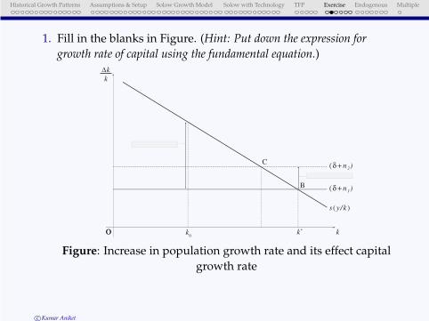
1. Fill in the blanks in Figure. (Hint: Put down the expression for
growth rate of capital using the fundamental equation.)
O
(δ+n 1)
s (y/k)
B
k
k
∆
(δ+n 2)C
kk*k0
O
Figure: Increase in population growth rate and its effect capital
growth rate
c©Kumar Aniket
Historical Growth Patterns Assumptions & Setup Solow Growth Model Solow with Technology TFP Exercise Endogenous Multiple
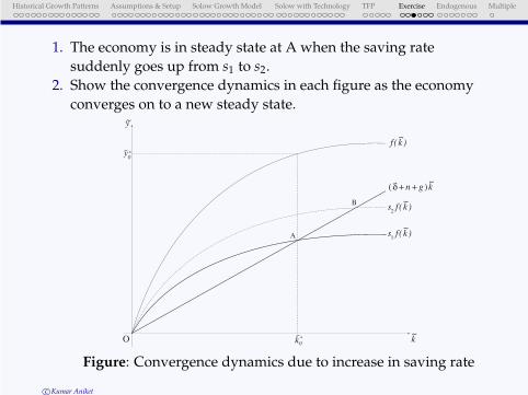
1. The economy is in steady state at A when the saving rate
suddenly goes up from s1 to s2.
2. Show the convergence dynamics in each figure as the economy
converges on to a new steady state.
O k
f(k)
y
k0
y0
A
(δ+n+g)k
s1 f (k)
s2 f (k)
~
~
~
~
~
~
~
B
~
*
*
Figure: Convergence dynamics due to increase in saving rate
c©Kumar Aniket
Historical Growth Patterns Assumptions & Setup Solow Growth Model Solow with Technology TFP Exercise Endogenous Multiple
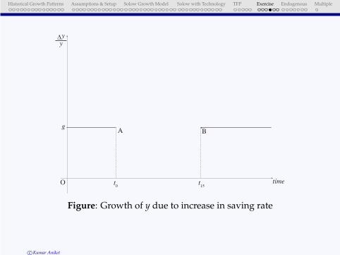
O time
gA
yy
∆
t0
B
t15
Figure: Growth of y due to increase in saving rate
c©Kumar Aniket

Historical Growth Patterns Assumptions & Setup Solow Growth Model Solow with Technology TFP Exercise Endogenous Multiple
Cobb Douglas production function
Y = Kα(AL)1−α
Per-worker production function
y = A1−α kα
Determining the growth rate of y
∆y
y= (1−α)
∆A
A+α
∆k
k
c©Kumar Aniket

Historical Growth Patterns Assumptions & Setup Solow Growth Model Solow with Technology TFP Exercise Endogenous Multiple
GROWTH RATES IN SOLOW
∆y
y= (1−α)
∆A
A+α
∆k
k
1. ∆AA = g
2. ∆kk = g (steady state)
⇒ ∆y
y= (1−α)g+α g = g
⊙ y grows at rate g in steady state because
◦ A always grows at the rate g
◦ k grows at the rate g in steady state
c©Kumar Aniket

Historical Growth Patterns Assumptions & Setup Solow Growth Model Solow with Technology TFP Exercise Endogenous Multiple
EXTERNALITIES OF INVESTMENT
Till now we have assumed that A grows at an exogenous rate g
Assumption (Positive Externalities of Investment)
The act of investment generates new ideas for both the investing firm and
other firms in the economy. Specifically,
A = λk (λ > 0)
stock of knowledge A is proportional to the stock of capital stock per worker k
⊙ Investing (k ↑) affects output y through two distinct channels:
◦ Direct effect: greater capital stock per worker lead to greater
output per worker
◦ Indirect effect: higher capital stock per worker leads to higher
value A which leads to higher output per worker.
c©Kumar Aniket

Historical Growth Patterns Assumptions & Setup Solow Growth Model Solow with Technology TFP Exercise Endogenous Multiple
THE TWO CHANNELS
⊙ Investing (k ↑) affects output y through two distinct channels:
◦ Direct effect: higher k leads to higher y
◦ Indirect effect: higher k leads to higher value of A which leads to
higher y.
y = (A)1−α kα = (λk)1−α kα = λ 1−α k
⇒ y
k= λ 1−α = constant ⇒ ∆y
y=
∆k
k
c©Kumar Aniket

Historical Growth Patterns Assumptions & Setup Solow Growth Model Solow with Technology TFP Exercise Endogenous Multiple
DERIVING ENDOGENOUS GROWTH
∆K
K= s · Y
K−δ
⇒ ∆k
k= s · y
k− (δ +n) = s ·λ 1−α − (δ +n)
◦ growth rate of k depends on the s,δ ,n and λ
c©Kumar Aniket
Historical Growth Patterns Assumptions & Setup Solow Growth Model Solow with Technology TFP Exercise Endogenous Multiple
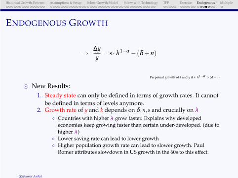
ENDOGENOUS GROWTH
⇒ ∆y
y= s ·λ 1−α − (δ +n)
Perpetual growth of k and y if s ·λ1−α > (δ +n)
⊙ New Results:
1. Steady state can only be defined in terms of growth rates. It cannot
be defined in terms of levels anymore.2. Growth rate of y and k depends on δ ,n,s and crucially on λ
◦ Countries with higher λ grow faster. Explains why developed
economies keep growing faster than certain under-developed. (due to
higher λ )
◦ Lower saving rate can lead to lower growth
◦ Higher population growth rate can lead to slower growth. Paul
Romer attributes slowdown in US growth in the 60s to this effect.
c©Kumar Aniket

Historical Growth Patterns Assumptions & Setup Solow Growth Model Solow with Technology TFP Exercise Endogenous Multiple
SUMMARY: ENDOGENOUS GROWTH
⊙ Externalities of capital investment create an extra channel
through which investment affects the output
⊙ Technological Progress is endogenised
◦ Stock of Knowledge A is proportional to capital stock per worker k
⊙ We get perpetual growth of k and y which depends on
◦ s,δ ,n
◦ the strength of externality of capital investment, namely the value
of λ◦ higher the value of λ , the faster the economy grows
⊙ r is constant and w grows at the rate at which k and y grows
c©Kumar Aniket

Historical Growth Patterns Assumptions & Setup Solow Growth Model Solow with Technology TFP Exercise Endogenous Multiple
1. Draw the following production function below
i. y = A · kα
ii. y = λ 1−α k
O k
y
k
y
Figure: Production Functions
c©Kumar Aniket

Historical Growth Patterns Assumptions & Setup Solow Growth Model Solow with Technology TFP Exercise Endogenous Multiple
1. Trace the path of the economy if it starts from capital stock k0.
O k
sλ 1−αk
y
(δ+n)k
k0
A
BC
D
E
k1
Figure: Endogenous growth with linear production function
c©Kumar Aniket

Historical Growth Patterns Assumptions & Setup Solow Growth Model Solow with Technology TFP Exercise Endogenous Multiple
k(t � 1) 45° k(t � 1) sf(k(t)) � (1 � •)k(t)
45°
sf(k(t)) � (1 � •)k(t)
0 0k(t) k(t)
A B
sf(k(t)) � (1 � •)k(t)k(t � 1) 45°
0k(t)
C
FIGURE2.5 Examples of nonexistence and nonuniqueness of interior steady stateswhenAssumptions 1and 2 are not satisfied.
c©Kumar Aniket