economic growth and the balance-of-payments constraint · economic growth and the...
TRANSCRIPT
1
Economic Growth and the Balance-of-Payments
Constraint
Dr John McCombie
Director
Cambridge Centre for Economic and Public Policy
University of Cambridge

2
Introduction
Approaches to economic growth
Two paradigms
• The neoclassical supply-oriented approach, based on the production function and full employment
• The Keynesian demand-oriented balance-of payments-constrained growth. Output may be less than full employment

3
The Balance of Payments
Current account:
Exports + Financial Flows Imports
X + F M
Confusingly, balance-of-payments equilibrium means X = M
Holds for countries (easily measured), regions and
individuals.
If M > X the region has to borrow (F) from other regions.

4
The Balance of Payments
The problem is that a country cannot go on borrowing
indefinitely. The debt (the sum of F) cannot go on
increasing for ever. Problem of the region or country
defaulting on the debt.

5
How can the balance-of-payments affect
economic growth?
Temporary shocks: The Asian financial crisis of 1997.
Long-term growth rates: UK in the 1950s & 1960s
Stop-go cycles.
Transmission of low growth in OCA ( e.g. The
Eurozone)
Regions also have balance-of-payments although there
are no statistics collected.
6
Problem with the Cumulative Causation Model
• A region or a country can go on exporting as much as it likes. But it will build up trade surpluses if exports exceed imports. Similarly, other countries may be accumulating net overseas debt, but this cannot go on forever. There must be some mechanism that brings the growth of exports and imports into equality.
• There is a balance-of-payments constraint (note that this also applies to regions in a common currency area).
The (weighted) growth exports + the growth of net financial flows =
the growth of imports (excluding the rate of change of relative prices)
If the growth of imports > growth of exports, net overseas debt will accumulate. But it cannot do this indefinitely.

7
Exchange Rate Adjustment Mechanism
If imports > exports
(i) Exchange rate adjusts to bring it back into equilibrium
(ii) Relative prices adjust in common currency union or regions
If either of these mechanisms is effective then there is no balance-of-
payments constraint.
Effectively, regional and national economies are “delinked”.

8
The Growth Rates of Countries are Interlinked
• The growth rates of even the advanced countries are inextricably linked – indeed the large OECD simulation macroeconomic model is known as the LINK model
• The beggar-my-neighbour policies of the advanced countries in the 1930s. “Exporting unemployment” by tariffs and quotas.
• Rapid post-war growth led by first the US and then Germany as the engine of growth. Rapid reduction of tariffs under GATT. It was the growth of world demand that became crucial for the Golden Age of 1950-1973
• UK stop-go policies 1950-1973 associated with balance-of-payments crisis. As output grows, so the current account deteriorates as imports increase rapidly, and exports grow at a constant rate determined by world demand.

• UK stop-go policies 1950-1973 associated with balance-
of-payments crisis.
• As output grows, so the current account deteriorates as
imports increase rapidly, and exports grow at a constant
rate determined by world demand.
Import growth determined by domestic output growth.
Exports determined by the (exogenous) growth of world
markets.
Output growth increases import growth (export growth
constant) growing current account deficit. Not
sustainable in the long run.
9

10
The Ineffectiveness of Floating Exchange Rates
• Once we move from considering the changes in the level of output, to the rate of growth, the role of the balance-of-payments becomes important, even with floating exchange rates.
• Changes in the nominal real exchange rate may be short lived because of a rapid-pass through of import prices and “real wage resistance”.
• The price elasticities may be low and the Marshall-Lerner conditions barely satisfied
– Advanced countries: non-price rather than price competitiveness matters
– Developing countries: price elasticities for primary commodities relative low.
• With Keynesian import and export demand functions, to increase or decrease the growth of exports and imports requires a continuous real depreciation of the exchange rate.

11
EMU & Common Currency Areas
• By definition these have a common currency and so no
exchange rate.
• Cost competitiveness can only be increased through a
reduction in the regional real wage. Difficult to achieve.
• Prices are determined on national markets
• Regions still have balance-of-payments although not
officially recorded as such.
• There are much greater fiscal transfers between regions but
these vary. Compare the US with the EMU.

12
Balance-of-Payments Constrained Growth
The cumulative causation model we discussed last time:
- criticized by Thirlwall himself (Thirlwall, 1979)
- Implicitly KDT model assumes (imports) M can grow permanently faster than (exports) X
- BUT, not true! The implied increasing foreign indebtedness will be ultimately unsustainable…
BoP constrained growth
consider the BoP constrained growth model

13
The Balance-of-Payments Constraint
“At the theoretical level, it can be stated as a fundamental proposition that no country can grow faster than the rate consistent with balance-of-payments equilibrium on current account unless it can finance ever-growing deficits, which in general it cannot”. (A. P Thirlwall)
• As a rule of thumb international financial markets become distinctly nervous if the overseas debt to GDP ratio exceeds around 50%. It does, however, depend on the size and level of development of the country concerned.

14

The growth of a country is said to be balance-of-payments
constrained if the growth rate consistent with a current
account equilibrium (or a sustainable growth of overseas
borrowing) is below the maximum growth of the economy
determined by the maximum growth of supply-side factors.
Growth of the supply side:
1. growth of the labour force
2. rate of capital accumulation (function of the growth of
output)
3. rate of technical progress (function of the growth of
output; Verdoorn law)
15
16
The Balance-of-Payments Equilibrium Growth
Model
Some Definitions
yP = the growth of productive capacity (maximum growth
rate)
yB = the balance-of-payments constrained growth rate
yA = the actual growth rate
yP > yB yA Balance-of-payments constrained growth
(lower rate of capital accumulation, technical
progress, disguised unemployment)
17
The Model
• Exports are a function of the income world market and relative prices. (Export demand function)
• Imports are a function of domestic income and relative prices. (Import demand function)
• Exports + net financial flows (long-term and short-term speculative flows) = imports (identity)
Let‟s express these in growth rates

18
The Balance-of-Payments Equilibrium Growth
Model
(1) Export demand equation
x = z - (pd - pz - er)
The growth of exports (x) is determined by the growth of world income (z)
and the rate of change of relative prices
(2) Import demand equation
m = y + (pd - pz - er)
The growth of imports (m) is determined by the growth of domestic
income (y) and the rate of change of relative prices.

19
The Balance-of-Payments Equilibrium Growth
Model
(3) Balance-of-payments identity
x + (1-)f m + pz – pd – er
The (weighted) growth of exports and the (weighted) growth
of capital flows must equal the growth of imports plus
the rate of change of prices in a common currency.

20
The Balance-of-Payments Equilibrium
Growth Model
(3) Balance-of-payments identity
x + (1-)f m
Suppose relative prices do not change, then if the growth of
imports is greater than export growth, there must
borrowing from abroad; hence the growth of capital
flows into the country.

21
Solution to the model
We substitute the three equations into each other and solve
for the growth of domestic income.
The growth of output y is determined by the growth of world
income z (as this determines the growth of exports x), the
rate of change of relative prices (relative price
competitiveness) and the growth of capital inflows f .
f)1()erpp)(1(zy
fd
B

22
Solution to the model
1. The first term is the effect of the exogenous growth of
world income.
2. The second teem gives the effect of the changes in relative prices.
3. The third term gives the effect of real capital inflows/outflows.
f)1()erpp)(1(zy
fd

23
Solution to the model
The balance-of-payments equation
But changes in relative prices have little effect on growth
rates of X and M because of (i) Marshall-Lerner
conditions just met or (ii) oligopolistic competition (iii)
national wage bargaining
f)1()erpp)(1(zy
fd
B
0)erpp)(1( fd
24
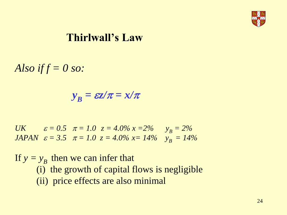
Thirlwall‟s Law
Also if f = 0 so:
yB = z/ = x/
UK = 0.5 = 1.0 z = 4.0% x =2% yB = 2%
JAPAN = 3.5 = 1.0 z = 4.0% x= 14% yB = 14%
If y = yB then we can infer that
(i) the growth of capital flows is negligible
(ii) price effects are also minimal

How do we interpret and ?
• These are the world income elasticity of demand for a
country’s exports () and the domestic income elasticity of
demand for imports ().
= 0.5 (UK) World income grows at 4%, UK exports grow at
2%
= 3 (Japan) World income grows at 4% , Japanese exports
grow at 12%.
They reflect differences in non-price competitiveness
(quality, delivery times, distribution networks etc.
Composition of exports)
25

26
The Key to Differences in Export Growth
The value of ; the world income elasticity of demand for a country’s exports. Differences reflect non-price competitiveness and the growth of demand for the exports as world income grows.
Why do these values vary between countries?
Composition of exports (not the advanced countries)
Quality, delivery times, characteristics of the goods.
Primary commodities
The value of , the domestic income elasticity of imports may vary. High for developing countries: imported advanced consumer goods and capital goods.

27
Theoretical foundations
The Dynamic Harrod Foreign Trade Multiplier
Simplest possible model. (With the usual notation.)
• Y = C + X (5)
• Y= C+ M (6)
• M= mY (7)
For expositional ease, following Harrod, we ignore investment, savings, government expenditure and taxation and relative prices.

28
The Dynamic Harrod Foreign Trade Multiplier
If X = M (equilibrium on the current account)
Y = X/m (8)
Y = (1/m)X (9)
Y/Y = (1/m)(X/Y)(X/X) (10)
But .......
(1/m)(X/Y) 1/
So.......
Y/Y = (X/X)/ or y = x/ (Thirlwall‟s Law)

29
The Hicks Super-multiplier
When we introduce other components of domestic demand ( I, G, etc), the effect of an increase is the Hicks super-multiplier which is:
(i) Harrod trade multiplier
plus
(ii) the effect of the relaxation of the balance-of-payments constraint that allows other components of domestic demand (I, G) to increase.

How does the BoP relate to the cumulative causation
model?
• Faster output growth leads to increasing price
competitiveness – may not be effective.
• Faster output growth leads to greater capital accumulation,
development of new goods etc, greater innovation, greater
non-price competitiveness (likely to be a very slow
adjustment process).
30

Recent Developments
• Nell’s generalisation of the model to many countries
South Africa; Rest of the Southern Africa Development
Community and the OECD.
• Araujo and Lima’s multi-sectoral model; composition of
imports and exports could be important. Those developing
countries that have closed the gap fastest have
concentrated on high income elasticity of demand goods
31
Fallacy of composition argument
Palley, etc
• Problem of identities
• Reciprocal nature of growth
• Applies to domestic output, and the individual
32
33
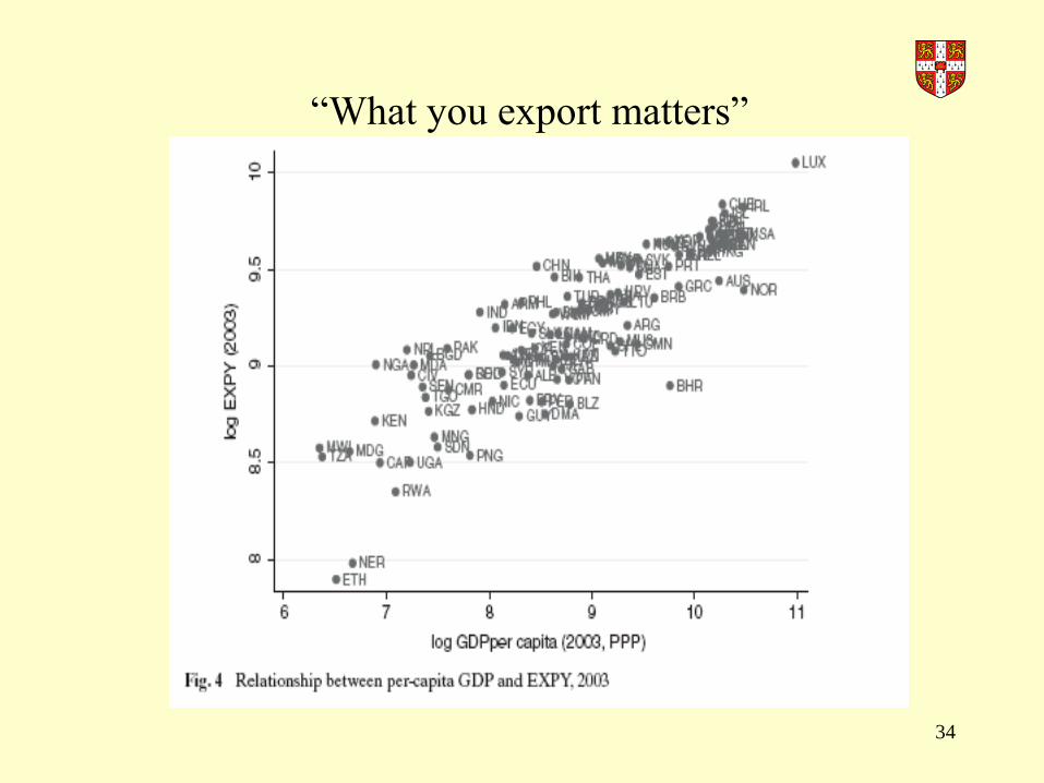
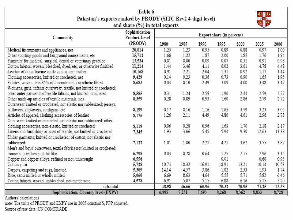
“What You Export Matters”. Rodrik, Dani; Hausmann,
Ricardo; Hwang, Jason
Journal of Economic Growth 2007.
Construct an index for export sophistication and find it is a
good predictor of per capita GDP
Take an export category; calculate each country’s
productivity and produce an index using the weighted
country figures. Then see the percentage of exports that a
country has in this export category. The initial level of this
variable is a very good predictor of a country’s subsequent
growth rate.
34
“What you export matters”

35
“What you export matters”

36
How does the law explain overall growth?
(i) the growth of exports increases the growth of output
through Harrod dynamic multiplier effects.
(ii) By initially relaxing the balance-of-payments constraint, it
allows other domestic components of expenditure to
increase, thereby increasing the balance-of-payments
deficit until it comes back into equilibrium.
Both effects are called the “Hick’s supermultiplier”

37
Calculations of the Growth Rate Consistent with
Balance-of-Payments Equilibrium 1951-1973
Country
Change in GDP
%
Change in
Exports (x)
%
Income
Elasticity
of Demand for
Imports ()
Balance of Payments
Equilibrium
Growth Rate
Austria 5.1 10.7 n.a. -
Belgium 4.4 9.4 1.94 4.84
Canada 4.6 6.9 1.20 5.75
Denmark 4.2 6.1 1.31 4.65
France 5.0 8.1 1.62 5.00
Germany 5.7 10.8 1.89 5.71
Italy 5.1 11.7 2.25 5.20
Japan 9.5 15.4 1.23 12.52
Netherlands 5.0 10.1 1.82 5.55
Norway 4.2 7.2 1.40 5.14
United Kingdom 2.7 4.1 1.51 2.71
U.S.A. 3.7 5.1 1.51 3.38

38
Balance-of-Payments Constrained Growth: An
Illustrative Example
Initial growth rates
yP yB m x
Group I 5% - 1.0 2.0 5% 10%
Group II 5% - 2.0 1.0 10% 5%
Balance-of-payments equilibrium growth rate
yP yB m x
Group I 5% 5% 1.0 2.0 5% 5%
Group II 5% 2.5% 2.0 1.0 5% 5%
The countries comprising Group I which is the more competitive trading bloc may be (i) resource constrained (ii) policy constrained. Its growth rate determines the growth of Group II which is balance-of-payments constrained.

39
• Pakistan’s growth rate was about 6% in the 1960s. In the 1970s and 1980s it became a rapidly industrialising country but never at the rate of growth of the Asian Tigers or China.
• Poverty reduction plan 7 to 7.5% growth per annum
• But problem of recurrent balance-of-payments crises.
• Latest was 2007-2008. Had to go to the IMF for a loan of $11.3 billion.
An Example: Is Pakistan‟s Growth Rate Balance-of-
Payments Constrained?

40
Pakistan Economic Survey (2007-08, p. xvi-xvii)
Pakistan’s exports suffer from serious structural
issues which need to be addressed primarily by the
industry itself, with government playing its role of
a facilitator. Textile is the backbone of Pakistan’s
exports but bears various tribulations.

41
These include:
(i) low value added and poor quality products fetching low international prices;
(ii) the machinery installed in recent years has depreciated considerably relative to Pakistan’s competitors;
(iii) these machines are power-intensive, less productive, and carry high maintenance cost;
(iv) augmented wastage of inputs adding to the cost of production;
(v) little or no efforts on the part of industry to improve their workers’ skills;
(vi) industry spending less money on research and development and;
(vii) export houses lacking capacity to meet bulk orders as well as meeting requirements of consumers in terms of fashion, design and delivery schedule.
42
Policy Implications
• Supply characteristics are important. Improve
• It is no use if Pakistan is able to manufacture, say,
cheap brass automobile radiators when technology
has moved on so that the leading world
automobile manufacturers are now using
aluminium radiators. (The exception is that
Pakistan can sell these radiators in its small
protected domestic market.)

43
Pakistan‟s Balance-of-Payments Constrained Equilibrium
Growth Rate
Sophisticated estimation puts this between 4% and 5% per
annum; well below the target rates.

44
Contribution of the Components of the Ex Post Balance-of-Payments Growth
Rate to the Actual Growth Rate: Pakistan, 1980-2007
Component
(A)
Weak Test
(B)
Strong Test
Exports,
xX ,
zX
88% (4.66 pp)
58% (3.06 pp)
Unrequited remittances,
)pr( XR 40% (2.11 pp) 40% (2.11 pp)
Real effective exchange rate,
)reer(,
)reer)(( X 12% (0.62 pp)
23% (1.23 pp)
Terms of trade,
)pp( MX -44% (-2.34 pp) -44% (-2.34 pp)
Financial flows,
)pf( XF 5% (0.26 pp)
24% (1.25 pp)
Total 100% (5.30) 100% (5.30)
Notes: The figures in parentheses are the contributions expressed as a percentage point growth rate (pp).
Columns may not sum to the value of the totals because of rounding errors.
45

46
Policy Implications
• Tariff protection to reduce , but needs a
sunset clause.
• Subsidies for exports, but needs a sunset
clause (problems of rent seeking)

47
Extending the Theoretical Model for an
Individual Country

48
The Country Growth Equation
The equation yB = z/ is an equilibrium locus. We need to introduce another element into the model.
From the traditional Keynesian income expenditure model we
have (ignoring the balance of payments): Income = (1/k)(Exports + Other Autonomous Expenditure) Y = (1/k)(X + A) where 1/k is the traditional Keynesian
multiplier. But exports are a function of world income so X = f(Z).

49
Thus, in terms of growth rates we have the growth of output:
y = f(autonomous expenditure growth) + g1(export growth)
y = f(autonomous expenditure growth) + g2(world income
growth or the growth of the other trading bloc).
In other words, the growth of income will increase if export
growth, investment growth, or the growth of government
expenditures increase.
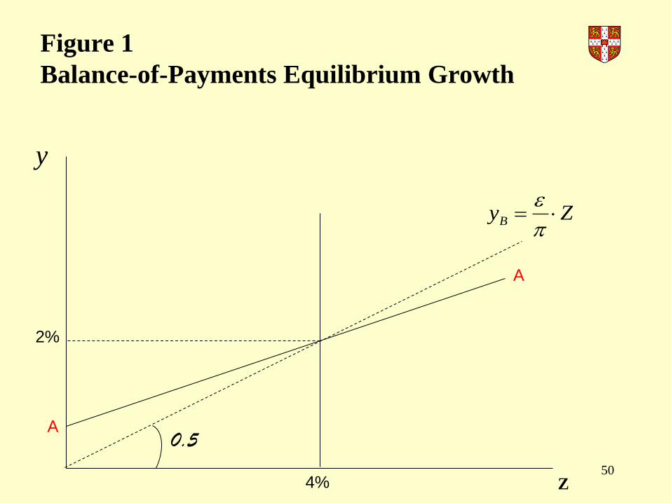
50
Figure 1
Balance-of-Payments Equilibrium Growth
ZyB
Z
A
A
2%
4%
y
0.5

51
Figure 2
An Increase in the Growth of Autonomous Expenditure
zyB
Z
Ao
Ao
4%
y
A1
A1
f

52
The working of the model
So let us suppose that the country is growing below its
potential and the government decides to increase the
growth of its expenditures through deficit financing. This
shifts the line AA upwards.
But this is unsustainable as it needs the rate of growth of
output given by f to be covered by the growth of financial
inflows.

53
Increase in non-price competitiveness
We can see how an increase in non-price competitiveness will
allow the country to increase its rate of growth without
encountering the balance-of-payments constraint.

54
zy0
0B
y
Z
A0
A0
4%
A1
A1
Figure 3
An Increase in Non-price Competitiveness
zy1
1B

55
A World Recession
We can see how if a major country reduces its
growth for policy reasons (e.g. to combat
inflation), it will induce a slower rate of growth of
the other countries because of the balance-of-
payments constraint.

56
zyB
y
Z 4%
Figure 4
The Effect of a World Recession
a
2%
1%
b 2%
f ’

57
Lifting the Balance-of-Payments Constraint:
Policy Implications
1. Currency Devaluation
2. More Capital Inflows
3. Import Restrictions
4. Structural Change
The Balance of Payments Does Not Look After Itself!

58
EMU problems are „balance-of- payments
problems‟
• Suppose a region suffers from a collapse of
demand for exports.
• To maintain the growth of standard of living
requires an ever increasing level of fiscal transfers.
• These may not be sufficient (EMU).
• The capacity of the country to borrow.
commercially from the rest of the currency area is
limited.

Readings
The PSL Quarterly Review, vol. 64, No 259 (2011)
http://bib03.caspur.it/ojspadis/index.php/PSLQuarterlyReview/issue/view/
370/showToc (All downloadable.)
“Balance of payments constrained growth models: history and overview”,
Anthony P. Thirlwall
“Criticisms and defences of the balance-of-payments constrained growth
model: some old, some new”, John S.L. McCombie
“The remarkable durability of Thirlwall’s Law”, Mark Setterfield
“The Balance of Payments Constraint as an Explanation of International
Growth Rate Differences”, Anthony P. Thirlwall
59