Economic Globalization, Mercantilism andEconomic Growth

Gaowang Wang∗

Central University of Finance and Economics

Heng-fu Zou†

Central University of Finance and Economics

April, 2012

Abstract

Obstfeld (1994) shows theoretically that international economicintegration accelerates economic growth of all countries in the world,which does not match the data very well. By introducing Zou (1994)’sviewpoints of mercantilism into the Obstfeld model, the paper showsthat the excessive pursuits for wealth heighthen the demand for finan-cial assets with high return and high risk in the global financial marketwhich distorts the mechanism of financial market promoting economicgrowth, and hence leads to different growth performances within dif-ferent countries. Specifically, for different economies, not only do thesame technology or preference shocks have different growth effects,but also economic integration has different growth effects.Keywords: Globalization, Economic Growth, MercantilismJEL Classification Numbers: C61, G11, F43

∗China Economics and Management Academy, Central University of Finance and Eco-nomics, Beijing, 100081, China. Email address: wanggaowang@gmail.com.†China Economics and Maganagement Acedamy, Central University of Finance and

Economics, Beijing, 100081, China. Email: zouhengfu@gmail.com

1

1 Introduction

In a stochastic model with heterogenous consumers who diversify financialportofolios globally, Obstfeld (1994) shows that financial openness enforcesan attended world portfolio shift from safe low-yield capital to riskier high-yield, specialized productive capitals and hence promotes all countries’eco-nomic growth in the world. Namely, economic globalization does good to allcountries in the world economy. Obstfeld (1994)’s research provides strongtheoretical supports for economic globalization, trade liberalization and fi-nancial openness. However, the theoretical results of Obstfeld (1994) doesnot accord very well with the economic facts on economic globalization since1960s.Dollar and Kraay (2001) provide plenty of data on economic globalization

which show that Obstfeld (1994)’s arguments may be misleading. From theaggragate data from 1960s to 1990s listed in table 3 in their paper, though theimprovements of degrees of openness of globalizers (increases of imports andexports and reductions of import tariffs) accelarate their economic growthrates (the ratios of trade to GDP of globalizers: 15.7% in 1960s, up to 16.0%in 1970s, to 24.75% in 1980s, and to 32.6% in 1990s; the levels of importtariffs of globalizers: 57.4% in 1980s, down to 34.5% in 1990s; growth ratesof GDP: 1.4% in 1960s, up to 2.9% in 1970s, to 3.5% in 1980s, and to 5.0%in 1990s), however, the improvements of degrees of openness of rich countriesbring about the reduction of economic growth (the ratios of trade to GDP ofrich countries: 20.5% in 1960s, up to 29.3% in 1970s, to 36.8% in 1980s, andto 50.0% in 1990s; the levels of trade to GDP: 14.6% in 1980s, down to 7.4%;the growth rates of GDP: 4.4% in 1960s, down to 3.6% in 1970s, to 2.6% in1980s, and to 2.4% in 1990s). From the cross-country data of 24 post-1980globalizers in table 1 and 2 in their paper, some countries gained more rapidgrowth from economic openness, such as Argentina, Bangladesh, China, Do-minican, Haiti, Hungary, India, Ivory Coast, Malaysia, Mexico, Nicaragua,Paraguay, and Zimbabwe etc.; some countries grew more slowly from eco-nomic openness, such as Colombia, Costa Rica, Jamaica, and Thailand etc.,and other countries kept the same paces as before, even though their degreesof openness were improved greatly. The economic data show that not allof the countries gain advantages from economic globalization because someeconomies keep their growth constant and some countries get worse fromeconomic openness. The divergence between the theoretical model and real

2

economic data reveals the failure of the Obstfeld (1994) model in explainingthe real effects of economic globalization. Meanwhile, it is also necessary todevelop appropriate models to expain the real economic data.How to explain these data? Actually, when referring to terminologies of

imports and exports, import tariffs and trade liberalization, we are likely toremind of mercantilism which attaches importance to trade protections andfavorable balances of trade opposite to liberalism. As an important genrein the history of economic thought, mercantilism dominated the mainstreamof the world economy in at least one half of 500 years after its emergencein the sixteen century. The conclusion can be drawn from the developmenthistory of mercantilism. Mercantilism experiences three rapid developmentalstages roughly from its emergence to the present: the first stage is from thesixteenth century to the end of the eighteenth century. In these 300 yearsor so, mercantism experiences the most rapid development. In this period,mercantilism deminated the western europe and led to the earliest developedcountries in the history such as Spain, Portugal, Germany, Poland, Russia,Sweden, France, Netherlands and Britain etc.. Namely, the modern europedid not grow up until the emergence and development of mercantilism.1Thesecond one is from the end of the nineteenth century to the second world war,in which neomercantilism came into being and grew. The prominent eventsof neomercantilism are that US and Germany surpassed UK who had begunto advocate free trade since the end of the eighteenth century successivelyand became the first and second economic powers at that time. Besides,by utilizing mercantilist policies Japan became the sole developed countryoutside the europe in the same period. The third one is from 1970s to thepresent, in which the outstanding events are the rapid growth of emergingmarket economies. Furthermore, ever since the breakout of 2009 financialcrises, in order to save the severe situation of native employment and weakeconomies, the developed countries headed by US adopted a large numberof protective policies, contrary to the export-oriented policies utilized byemerging market economies (EMEs) in the long run. It seems like thatmercantilism begins to renew its influence in the global economy. Altogether,mercantilism dominated the world economy in the most of 500 years fromits emergence. Because of this observation, we conjecture that it will behelpful to explain the real data of economic globalization by introducingmercantilism.

1A detailed recount of the first stage of mercantilism is in Cameron (1993).

3

Then, how to introduce mercantilism? We review the literature on mer-cantilism at first. It will be appropriate to divide the theoretical litera-ture into two parts roughly. Before 1960s, almost all great economists everworked on mercantilism, such as Adam Smith, John Maynard Keynes, JosephSchumpter, Jacob Viner and Eli Heckscher etc.. Their researches focused ondescribing phenomena, theoretical analysis and citing literature. However, notheoretical models were developed. From 1960s to the present, some mathe-matical models on mercantilism have been constructed. In the framework ofKeynesian economics, Samuelson (1964) put forward the first mathematicalmodel of mercantilism. He argued that “with employment less than full andnet national product suboptimal, all the debunked mercantilistic argumentsturn out to be valid. Tariff can then reduce unemployment, can add to theNNP, and increase the total of real wages earned”. Based on strategic tradetheory, Irwin (1991) points out that the reason why Dutch gained the strate-gic advantages over Britain in the east india trade is that Dutch harnessedpolitical power and privileges to commercial purposes and hence made himthe Stackelberg leader. Irwin (1991) argues that export subsidies do good tothe native economy. From the viewpoint of mercantilism as a fiscalism, Mc-dermott (1999) points out that the development of mercantilism is harmfulfor the long-run economic growth. In order to attain more fiscal revenues,government will adopt the mercantilist policy of controlling the degree ofopenness which will damage human capital accumulation, and hence long-run growth and convergence to the developed economies. In a framework ofmodern theory of international finance, Zou (1997) models the central themeof mercantilism, i.e., power and plenty, and points that an increase of thespirit of mercantilism or import tariffs will increase the long-run capital ac-cumulation and aggregate level of consumption. Aizenman and Lee (2007)identify the contributions of precautionary and mercantilist motives to thehoarding of international reserves in developing countries. The empirical partof their paper shows that the precautionary motive accounts for the majorpart of the high levels of reserves and the mercantilist motive just accounts forthe minor part; the theoretical part provides a particular mechanism for theempirical result: the large precautionary demand for international reservesis a kind of self-insurance for “sudden stops”. And Durdu et al. (2009) drawthe similar result to Aizenman and Lee (2007) in a framework of stochasticdynamic general equilibrium. In the paper, we adopt Zou (1997)’s modellingstrategy of mercantilism to explain the real economic data on globalization.By introducing Zou (1997)’s viewpoints on mercantilism into the Obst-

4

feld (1994) model, the paper shows that the excessive pursuits for wealthheighthen the demand for the financial assets with high return and high riskin the global financial market which distorts the mechanism of the finan-cial market promoting economic growth, and hence leads to different growthperformances within different countries. Specifically, for different economies,not only do the same technology or preference shocks have different growtheffects, but also economic integration has different growth effects. The pa-per not only explains the real economic facts and promotes us to reexaminethe economic aftermaths of the blind globalization, but also provides a newframework for explaining the diversity of the global economic growth2.The second section of this paper gives the individual choice in a closed

economy. In section 3, we discuss the equilibrium of the closed economy andthe results of comparative statics. In section 4, we examine the economiceffects of international economic integration and the diversity of economicgrowth. In section 5, we summarize the main findings and give some policysuggestions.

2 Individual Choice in a Closed Economy

In the beginning, we consider a closed economy with uncertainty. There existsa single good. The closed economy is populated by identical infinitely-livedindividuals who face consumption and savings decisions. At each moment t,the objective function U(t) of the representative individual is given by therecursion implicitly

f [(1−R)U(t)] =

(1−R1− 1

ε

)[C(t)W (t)θ

]1− 1ε h+ e−δhf [(1−R)EtU(t+ h)] ,

(1)where f(x) is defined by

f(x) =

(1−R1− 1

ε

)x1− 1ε1−R . (2)

In equation (1), Et is a mathematical expectation operator conditional ontime-t information, C(t) is time-t consumption, W (t) is time-t wealth. Sim-

2The famous literature of explaining the diversities of economic growth includes Romer(1986, 1990), Lucas (1988), and Grossman and Helpman (1991), Razin, Sadka and Yuen(2000), Jalles (2009), and Chen (2012) etc..

5

ilar to Zou (1997), the utility from consumption can be understood as ameasure of opulence and plenty in the words of Viner (1948), and the utilityfrom wealth as the power a nation possesses and enjoys. θ (> 0) stands forthe development degree of mercantilism, and the larger θ corresponds to thehigher degree. From equations (1) and (2), we can derive the utility functionU(t) as follows

U(t) =

[(C(t)W (t)θ

)1−R

1−R

] 1− 1ε1−R

h+ e−δh [EtU(t+ h)]1− 1ε1−R

1−R1− 1ε

, (3)

where the parameters R (> 0) and ε (> 0) measures the household’s relativerisk aversion (RRA) and its elasticity of intertemporal substitution (EIS).If R = 1

εholds, f(x) = x, and (3) degenerates as the standard time- and

state-separable expected-utility setup.3

Different from Eaton (1981) and Obstfeld (1994), for simplicity, we as-sume that there exist two kinds of assets: a risk-free asset with an exoge-nously given positive rate of return i and a risky asset with an instantenousexpected rate of return α > i and standard deviation σ > 0. It is assumedthat the individuals make investment decision using both of these two assetsand consumption and assets can be transformed into each other one-to-onewith zero cost. Moreover, it is assumed that there is no nondiversifiable in-come (such as labor income) which means that assets markets in this closedeconomy are complete. Let V B(t) denote the cumulative time-t value of aunit of output invested in riskless assets at time 0 and V K(t) the cumu-lative time-t value of a unit of output invested in risky assets at time 0.Explicitly, V B(0) = V K(0) = 0. With payouts re-invested and continuouslycompounded, V B(t) obeys the ordinary differential equation

3The more general preference setup of the non-expected utility function was proposedby Epstein and Zin (1989, 1991) and Weil (1989, 1990). It is problematic for the usualexpected utility function in which the coeffi cient of relative risk aversion is the reciprocalof the elasticity of intertemporal substitution, since the elasticity of substitution revealingthe relationships between interest rate and consumption growth is a dynamic concept withrespect to time, whereas the coeffi cient of relative risk aversion reflecting the risk attitudeof people is a static concept. Essentially, they have nothing to do with each other. The twoadvantages for considering such preferences are examining dynamic welfare comparisonscorrectly and finding how preference parameters influence the long-run economic growth.

6

dV B(t) = iV B(t)dt, (4)

and V K(t) obeys the geometric diffusion process

dV K(t)

V K(t)= αdt+ σdz(t). (5)

Thereinto, dz(t) is a standard Wiener process, such that z(t) = z(0) +∫ ts=0

dz(s), and σ2 is the instantaneous variance of returns. Actually, wecan look down upon (4) and (5) as two exogenously given “production”tech-nologies: (4) is a risk-free production technology and (5) a risky productiontechnology.Per capita wealthW (t) is the sum of per capita holdings of the composite

safe asset, B(t), and per capita holdings of risky asset, K(t):

W (t) = B(t) +K(t). (6)

Equations (4), (5), and (6) imply that

dW (t) = iB(t)dt+ αK(t)dt+ σK(t)dz(t)− C(t)dt. (7)

Let ω(t) denote the fraction of wealth invested in risky capital, and 1−ω(t)the fraction of wealth in risk-free assets. Then, an alternative way to write(7) is as

dW (t) = ω(t)α + [1− ω(t)]iW (t)dt+ ω(t)σW (t)dz(t)− C(t)dt. (8)

The individual’s optimization problem can be formulized as follows: max-imize (3) and subject to wealth accumulation equation (8) and the initialcondition W (t) = Wt. It is easy to know that the utility function given by(3) is ordinally equivalent to the following continuous form

U(t) = Et

∫ ∞s=t

f(Cs,Ws, Us)ds, (9)

where 2

f(Cs,Ws, Us) =

(CW θ

)1− 1ε − δ [(1− r)Us]

ε−1ε(1−R)(

1− 1ε

)[(1−R)Us]

ε−1ε(1−R)−1

.

7

Let J(Wt) denote the maximum feasible level of lifetime utility whenwealth at time t equals Wt. Itô’s lemma shows that the correspondingHamiltonian-Jacob-Bellman (HJB) equation is

0 = maxC,ω

(CW θ

)1− 1ε − δ [(1− r)Us]

ε−1ε(1−R)(

1− 1ε

)[(1−R)Us]

ε−1ε(1−R)−1

+ J ′(W ) [ω(α− i)W + iW − C] +1

2J ′′(W )ω2σ2W 2

.

The first-order conditions with respect to C and ω follow:

C = J ′(W )−ε [(1−R)J ]1−εR1−R W θ(ε−1), (10)

ω = − J ′(W )

J ′′(W )W

α− iσ2

. (11)

Substituting equations (10) and (11) into HJB equation gives rise to

0 =ε

ε− 1J ′1−ε [(1−R)J ]

1−εR1−R θθ(ε−1) − εδ

ε− 1(1−R)J + (12)

J ′− J

′

J ′′(α− i)2

σ2+ iW − J ′−ε [(1−R)J ]

1−εR1−R W θ(ε−1)

+

1

2

J ′2

J ′′(α− i)2

σ2.

The objective function suggests a guess that maximized lifetime utility Uis given by

J(W ) = AW (1+θ)(1−R). (13)

Then, J ′ = A(1 + θ)(1−R)W (1+θ)(1−R)−1, J ′′ = A(1 + θ)(1−R)[(1 + θ)(1−R)− 1]W (1+θ)(1−R)−2. Substituting (13) into (12) leads to

[A(1−R)]1−ε1−R (1+θ)1−ε = εδ−(ε−1)(1+θ)

[i− 1

[(1 + θ)(1−R)− 1]

(α− i)2

2σ2

]≡ µ.

(14)Similar to Merton (1971) and Obstfeld (1994), in order to guarantee the

existence of optimality, we assume that

µ > 0. (15)

8

Equation (15) tells that the parameters ought to satisfy the following twoconditions:

[A(1−R)]1−ε1−R > 0, (16)

εδ − (ε− 1)(1 + θ)

[i− 1

[(1 + θ)(1−R)− 1]

(α− i)2

2σ2

]> 0. (17)

Substituting (13) into (10) gives

C = [A(1−R)]1−ε1−R (1 + θ)1−εW ≡ µW. (18)

(18) and (15) show that the optimal consumption-wealth ratio is a posi-tive constant µ. If mercantilism is not introduced, it returns to Obstfeld(1994): µ = ε

δ −2 (1− 1

ε)[i+ (α−i)2

2σ2

]; if R = 1

εholds, it returns to Mer-

ton (1971): µ = 1R

δ − (1−R)

[i+ (α−i)2

2σ2

]. Substituting equation (13)

into (11) results in

ω =1

[1− (1 + θ)(1−R)]

α− iσ2

. (19)

From (19), on one hand, similar to Merton (1969, 1971) and Obstfeld (1994),the portfolio weight deponds not on the elasticity of intertemporal substitu-tion but on risk attitudes and production technologies; on the other hand,different from them, the portfolio weight also depends on the developmentdegree of mercantilism. Obviously, if no mercantilism, i.e., θ = 0, then weget back to the formula derived by Merton (1969, 1971) and Obstfeld (1994):ω = α−i

Rσ2.

3 Closed-Economy Equilibrium and Compar-ative Statics

3.1 Closed-Economy Equilibrium

Equilibrium growth in this closed economy can now be described. Thereexists several possibilities about the equilibrium portfolio choice. First ofall, a possibility is that ω > 1, which means that the closed economy wishes

9

to go short in risk-free assets in the aggregate. When the initial supplyof risk-free assets is excessive, this type of equilibrium may occur. And insuch equilibrium, from (19), we know that R > θ

1+θ, and α > i + σ2[1 −

(1 + θ)(1 − R)]. The possible reason for occurrence of this equilibrium isthat the yields of the risk-free assets are too low in the beginning of theeconomy. And in this equilibrium, the return of risk-free assets will rise,until α = i+ σ2[1− (1 + θ)(1−R)], i.e., ω = 1. Secondly, ω < 0 is possible.From (19), R < θ

1+θ. In this case, the coeffi cient of the relative risk aversion is

small and people want to sell short risky assets. The reason for this possibilityis that the risk of risky assets approaches infinite. Finally, ω ∈ (0, 1). In thisequilibrium, people possess both risky and risk-free assets. In the following,it is assumed that the former two cases do not occur.Equations (8) and (18) tell that

dW = [ωα + (1− ω)i− µ]Wdt+ ωσWdz. (20)

Equations (18) and (20) result in

dC = [ωα + (1− ω)i− µ]Cdt+ ωσCdz. (21)

Define g as the instantaneous expected growth rate of consumption, g ≡Et[dC(t)dt]

C(t). Equation (21) shows that g is endogenously determined as the

average expected return on wealth, ωα+(1−ω)i, less the ratio of consumptionto wealth, µ. Combination of (14) and (19) leads to a closed-form expressionfor the expected consumption growth rate,

g = [1 + (ε− 1)(1 + θ)] i− εδ +[2 + (ε− 1)(1 + θ)]

[1− (1 + θ)(1−R)]

(α− i)2

2σ2. (22)

Certainly, if θ = 0, we get back to Obstfeld (1994): g = ε(i−δ)+(ε+1) (α−i)22Rσ2

.

3.2 Comparative Statics

In the following, we begin to examine the long-run effects on consumptiongrowth and consumption-wealth ratio of all sorts of changes of exogenousparameters.

10

3.2.1 The Effects of Changes of Expected Rate of Return of RiskyAssets

Taking derivatives w.r.t α in (22) gives

dg

dα=

[2 + (ε− 1)(1 + θ)]

[1− (1 + θ)(1−R)]

(α− i)σ2

. (23)

Different from Obstfeld (1994), we can not determine the sigh of the deriv-ative in equation (23). Taking derivative on equation (23) w.r.t θ gives riseto

d(dgdα

)dθ

=(1 + ε)− 2R

[1− (1 + θ)(1−R)]2α− iσ2

> 0, 1 + ε > 2R= 0, 1 + ε = 2R< 0, 1 + ε < 2R

. (24)

Furthermore, we have(dg

dα

)θ>0

> 0, 1 + ε ≥ 2R

in det ermin ate, 1 + ε < 2R. (25)

When 1 + ε ≥ 2R holds,(dgdα

)θ>0−(dgdα

)θ=0

> 0. Comparing with theObstfeld (1994) economy without mercantilism, the consumption growth rateis even bigger when a positive technology shock occurs. We call the newlyaddition of the growth rate “mercantilist premium”and the correspondingarea of parameters “mercantilist area”, namely, MPα ≡

(dgdα

)θ>0−(dgdα

)θ=0,

MAα ≡

(ε, R) ∈ R2+ : 1 + ε ≥ 2R

. However, the sign of

(dgdα

)θ>0

can not bedetermined in MAα ≡

(ε, R) ∈ R2

+ : 1 + ε < 2R. Because of the existence

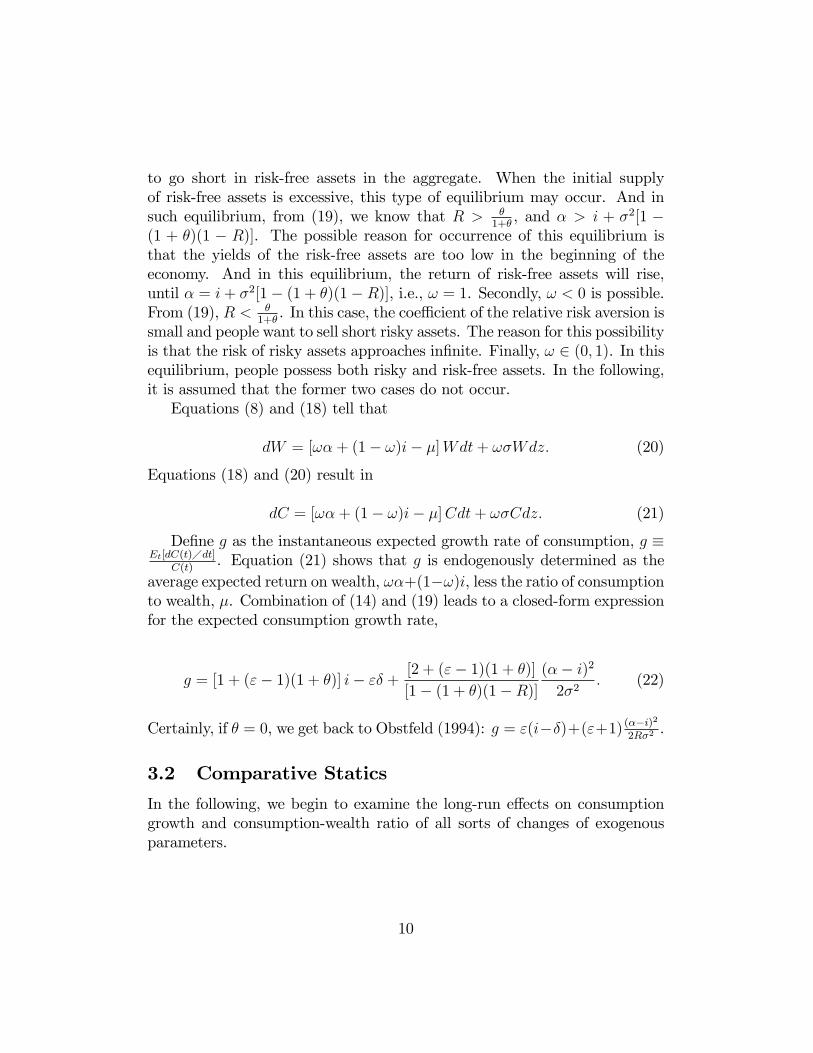
of mercantilism, the growth effects of technology shock depend on parametervalues of the elasticity of intertemporal substitution and the coeffi cient ofrelative risk aversion. Comparing with the Obstfeld (1994) model, if theparameter values are in “mercantilist area”, the consumption growth ratewill be even bigger; however, if not in “mercantilist area”, the sign of thederivative in equation (25) can not be determined, namely, the consumptiongrowth rate may increase, decrease or keep constant. Actually, (25) tellsus that if the elasticity of intertemporal substitution is large, mercantilismmagnifies the positive growth effect of the positive technology shock, whereasmercantilismmaymagnify, reduce or keep the positive effect of the technologyshock. The drop shadow part of figure 1 gives the “mercantilist aera”.(insert figure 1 here)

11

Taking derivative on equation (14) w.r.t α results in

dµ

dα=

[(ε− 1)(1 + θ)]

[(1 + θ)(1−R)− 1]

α− iσ2

. (26)

If there exists no mercantilism, i.e., θ = 0, we get back to Obstfeld (1994),namely,

(dµ

dα

)θ=0

=1− εR

α− iσ2

> 0, ε < 1= 0, ε = 1< 0, ε > 1

. (27)

However, by taking derivative on equation (26) w.r.t θ, we obtain

d( dµdα

)

dθ=

1− ε[(1 + θ)(1−R)− 1]2

α− iσ2

> 0, ε < 1= 0, ε = 1< 0, ε > 1

,

moreover,

(dµ

dα

)θ>0

=

>(dµdα

)θ=0

> 0, ε < 1

=(dµdα

)θ=0

= 0, ε = 1

<(dµdα

)θ=0

< 0, ε > 1

. (28)

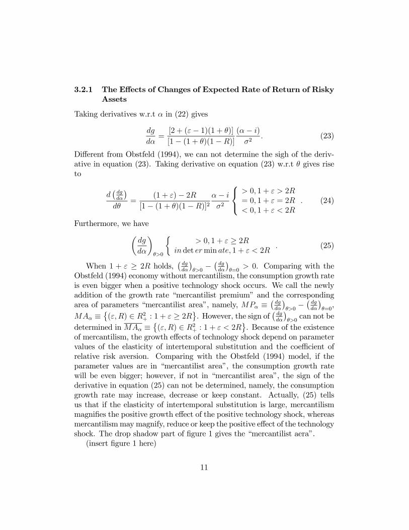
Comparing (28) with (27), we find that the signs of consumption-wealthratio affected by expected rate of return are both determined by whether theelasticity of intertemporal substitution large than one: a rise in the real rate ofreturn lowers consumption-wealth ratio when ε > 1, but raises it when ε < 1.Different from (27), (28) shows that though θ does not dominate the directionof the change of consumption-wealth ratio, mercantilism always magnifiesthese effects. Specifically, if ε > 1, consumption-wealth ratio becomes largerbecause of the increase of the real rate of return. The drop shadow part offigure 2 indicates the area of parameter where both consumption-wealth ratioand consumption growth rate are magnified by the existence of mercantilism:

(ε, R) ∈ R2+ : 1 + ε < 2R, ε < 1

.

(insert figure 2 here)

3.2.2 The Effects of Changes of Risk of Risky Assets

By taking derivative on equation (22) w.r.t σ, we have

12

dg

dσ= − [2 + (ε− 1)(1 + θ)]

[1− (1 + θ)(1−R)]

(α− i)2

σ3. (29)

If θ = 0, we go back to Obstfeld (1994), i.e.,(dg

dσ

)θ=0

= −ε+ 1

R

(α− i)2

σ3< 0. (30)

Since the sigh of the derivative in (29) can not be determined directly, bytaking derivative w.r.t θ, we have

d(dgdσ

)dθ

= − (ε+ 1)− 2R

[1− (1 + θ)(1−R)]2(α− i)2

σ3

< 0, ε+ 1 > 2R= 0, ε+ 1 = 2R> 0, ε+ 1 < 2R

. (31)

Combination of (30) and (31) leads to(dg

dσ

)θ>0

< 0, ε+ 1 > 2R

in det ermin ate, ε+ 1 < 2R. (32)

Different from the negative growth effect of the risky technology examinedby Obstfeld (1994), (33) shows that how the long-run growth rate respondsto risk shocks of risky assets depends on the values of preference parameters.If ε+ 1 > 2R, an increase of the risk of risky assets will decrease the growthrate of the economy, and the existence of mercantilism aggravates this effect(since

(dgdσ

)θ>0

6(dgdσ

)θ=0

< 0); if ε+ 1 < 2R, the direction is indeterminate.To examine the long-run effect on consumption-wealth ratio of the changes

of σ, by taking derivative on (14) w.r.t σ, we get

dµ

dσ=

(1− ε)(1 + θ)

[(1 + θ)(1−R)− 1]

(α− i)2

σ3. (33)

If θ = 0, it returns to Obstfeld (1994), namely,

(dµ

dσ

)θ=0

=(ε− 1)

R

(α− i)2

σ3

< 0, ε < 1= 0, ε = 1> 0, ε > 1

. (34)

Moreover, taking derivative on (34) w.r.t θ results in

13

d(dµdσ

)dθ

=ε− 1

[(1 + θ)(1−R)− 1]2(α− i)2

σ3

< 0, ε < 1= 0, ε = 1> 0, ε > 1

. (35)

Combination of (34) and (35) tells us that

(dµ

dσ

)θ>0

=

<(dµdσ

)θ=0

< 0, ε < 1

=(dµdσ

)θ=0

= 0, ε = 1

>(dµdσ

)θ=0

> 0, ε > 1

. (36)

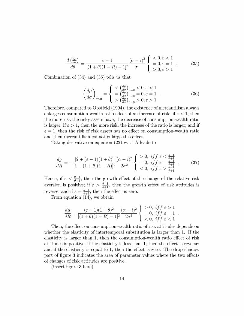
Therefore, compared to Obstfeld (1994), the existence of mercantilism alwaysenlarges consumption-wealth ratio effect of an increase of risk: if ε < 1, thenthe more risk the risky assets have, the decrease of consumption-wealth ratiois larger; if ε > 1, then the more risk, the increase of the ratio is larger; and ifε = 1, then the risk of risk assets has no effect on consumption-wealth ratioand then mercantilism cannot enlarge this effect.Taking derivative on equation (22) w.r.t R leads to

dg

dR= − [2 + (ε− 1)(1 + θ)]

[1− (1 + θ)(1−R)]2(α− i)2

2σ2

> 0, iff ε < θ−1

θ+1

= 0, iff ε = θ−1θ+1

< 0, iff ε > θ−1θ+1

. (37)

Hence, if ε < θ−1θ+1, then the growth effect of the change of the relative risk

aversion is positive; if ε > θ−1θ+1, then the growth effect of risk attitudes is

reverse; and if ε = θ−1θ+1, then the effect is zero.

From equation (14), we obtain

dµ

dR=

(ε− 1)(1 + θ)2

[(1 + θ)(1−R)− 1]2(α− i)2

2σ2

> 0, iff ε > 1= 0, iff ε = 1< 0, iff ε < 1

.

Then, the effect on consumption-wealth ratio of risk attitudes depends onwhether the elasticity of intertemporal substitution is larger than 1. If theelasticity is larger than 1, then the consumption-wealth ratio effect of riskattitudes is positive; if the elasticity is less than 1, then the effect is reverse;and if the elasticity is equal to 1, then the effect is zero. The drop shadowpart of figure 3 indicates the area of parameter values where the two effectsof changes of risk attitudes are positive.(insert figure 3 here)

14

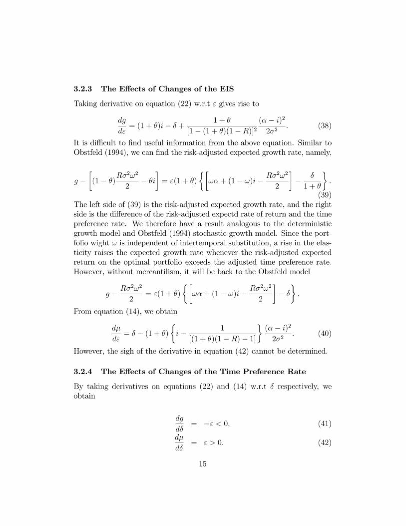
3.2.3 The Effects of Changes of the EIS

Taking derivative on equation (22) w.r.t ε gives rise to

dg

dε= (1 + θ)i− δ +

1 + θ

[1− (1 + θ)(1−R)]2(α− i)2

2σ2. (38)

It is diffi cult to find useful information from the above equation. Similar toObstfeld (1994), we can find the risk-adjusted expected growth rate, namely,

g −[(1− θ)Rσ

2ω2

2− θi

]= ε(1 + θ)

[ωα + (1− ω)i− Rσ2ω2

2

]− δ

1 + θ

.

(39)The left side of (39) is the risk-adjusted expected growth rate, and the rightside is the difference of the risk-adjusted expectd rate of return and the timepreference rate. We therefore have a result analogous to the deterministicgrowth model and Obstfeld (1994) stochastic growth model. Since the port-folio wight ω is independent of intertemporal substitution, a rise in the elas-ticity raises the expected growth rate whenever the risk-adjusted expectedreturn on the optimal portfolio exceeds the adjusted time preference rate.However, without mercantilism, it will be back to the Obstfeld model

g − Rσ2ω2

2= ε(1 + θ)

[ωα + (1− ω)i− Rσ2ω2

2

]− δ.

From equation (14), we obtain

dµ

dε= δ − (1 + θ)

i− 1

[(1 + θ)(1−R)− 1]

(α− i)2

2σ2. (40)

However, the sigh of the derivative in equation (42) cannot be determined.

3.2.4 The Effects of Changes of the Time Preference Rate

By taking derivatives on equations (22) and (14) w.r.t δ respectively, weobtain

dg

dδ= −ε < 0, (41)

dµ

dδ= ε > 0. (42)

15

The intuitive results in (41) and (42) are the same as Obstfeld (1994).An increase of the time preference rate affects both the growth rate andconsumption-wealth ratio with the same degree but opposte directions. Withthe larger time preference rate, people have less patience and incline to con-sume ahead of time. Hence, the long-run growth rate is even low and theoptimal consumption-wealth ratio is larger.

3.2.5 The Effects of Changes of the Spirit of Mercantilism

Taking derivative on equation (22) w.r.t θ results in

dg

dθ= (ε− 1) i+

(ε+ 1)− 2R

[1− (1 + θ)(1−R)]2(α− i)2

2σ2, (43)

the sign of which cannot be determined. However, if the parameter values ofthe elasticity of intertemporal substitution and the relative risk aversion sat-isfy both ε > 1 and ε+ 1 > 2R, then an increase of the spirit of mercantilismwill increase the economic growth; if the parameter values satisfy both ε < 1and ε + 1 < 2R, then an increase of the spirit of mercantilism will decreasethe economic growth.From equation (14), we have

dg

dθ= (1− ε)

[i+

(α− i)2

2σ2

]< 0, ε > 1= 0, ε = 1> 0, ε < 1

.

Hence, an increase of the spirit of mercantilism will (i) decrease consumption-wealth ratio whenever ε > 1, (ii) increase consumption-wealth ratio wheneverwhenever ε < 1, and (iii) have no effect on the ratio whenever ε = 1. Takingderivative on equation (19) w.r.t θ gives

dω

dθ=

1−R[1− (1 + θ)(1−R)]2

α− iσ2

> 0, R < 1= 0, R = 1< 0, R > 1

.

Then, an increase of the spirit of mercantilism will (i) increase the wealthweight invested in risky assets whenever R < 1, (ii) decrease the wealthweight invested in risky assets, and (iii) have no effect on the investmentbehavior of the individuals. Equation (19) shows that the portfolio weighton risky assets depends on the value of the coeffi cient of relative risk aversion

16

reversely. And the above result tells that the effect of portfolio choice ofmercantilism also depends on individual’s risk attitude: an increase of thedevelopment of mercantilism will increase the wealth weight on risky assetswhenever the relative risk aversion is low, and vice versa.Altogether, if the values of the elasticity of intertemporal substitution and

relative risk aversion satisfy M =

(ε, R) ∈ R2+ : ε > 1, ε+ 1 > 2R,R < 1

(the drop shadow part of figure 4), the spirit of mercantilism has positiveeffects on both the long-run rate of economic growth and consumption-wealthratio.(insert figure 4 here)

3.2.6 Brief Summary-Indeterminacy of Comparative Statics

The results of comparative statics in the closed economy are different fromObstfeld (1994) largely. Obstfeld (1994) shows that the growth effects oftechnological and preference shocks can be determined easily. However, be-cause of the existence of mercantilism, the effects of those shocks rely onparameter values of elasticity of intertemporal substitution, coeffi cients ofrelative risk aversion and spirit of mercantilism. In order to state this phe-nomena formally, we call this kind of indeterminacy of comparative staticsas indeterminacy of economic growth.4In the following open economy case,by introducing heterogeneity of consumers, we will discuss the diversity ofeconomic growth, which corresponds to indeterminacy of economic growthin the closed economy.Substituting equations (14) and (22) into (13) leads to the expression for

optimal social welfare

J(W ) =

[εδ − (ε− 1)(1 + θ)(i+ g + εδ)

2 + (ε− 1)(1 + θ)

] 1−R1−ε(W 1+θ(1 + θ)

)1−R

1−R . (44)

From (44), a useful property of the economy should be noted: when theeconomy holds both types of capital, the technology parameters α and σinfluence the individual’s lifetime utility only through their effects on thegrowth rate, g. The property of the model turns out to be useful in evaluatingthe growth effects of international asset-market integration.

4The indeterminacy defined here is different from the definition of multiple convergentpaths put forward by Benhabib and Perli (1994), and Benhabib and Farmer (1994).

17

4 Global Economic Integration and EconomicGrowth

4.1 Global Equilibrium in an Open Economy

All of the discussion above can be extended to a multicountry world economy.Since Merton (1971)’s mutual-fund theorem is still held in the framework ofmulticountry open economies, we can not only transform the discussion onindeterminacy of economy growth in the closed economy into the discussionon the diversity of economic growth in the open economy, but also examinethe diverse effect on economic growth of international economic integration.Let there be N countries, indexed by j = 1, 2, ..., N . Each country has a

representative resident with preferences of the form specified in (1) and (2) orin (3). However, preferences may be country-specific. Country j’s represen-tative individual has a RRA coeffi cient Rj, an EIS εj, a time preference rateδj, and the spirit of mercantilism θj. Hence, the representative individual ofcountry j has the utility function form

U j(t) =

[(Cj(t)Wj(t)

θj)1−Rj

1−Rj

] 1− 1εj

1−Rj

h+ e−δjh[EtU

j(t+ h)] 1− 1

εj1−Rj

1−Rj1− 1

εj

.

(45)Assume that there exists only one safe asset and its rate of return i∗ is

common to all countries. Each country j has only one risky asset and thecumulative value of a unit investment in country j’s risky capital follows thegeometric diffusion

dV Kj (t)

V Kj (t)

= αjdt+ σjdzj(t), j = 1, 2, ..., N. (46)

It is assumed that N country-specific technology shocks follow the instanta-neous correlation structure

dzjdzk = ρjkdt, j, k = 1, 2, ..., N. (47)

Similar to Svensson (1989) and Obstfeld (1994), the optimal vector ofportfolio weights for N risky assets of an individual from country j can be

18

derived as follows:

ωj ≡ (ωj1, ωj2, ..., ωjN)′ =Ω−1(α− i∗e)

[1− (1 + θj)(1−Rj)], (48)

whereωj ≡ (ωj1, ωj2, ..., ωjN)′ stands for the optimal portfolio for N risky assets

of the representative individual of country j;

Ω =[σjσkρjk

]N×N =

σ2

1 σ1σ2ρ12 ... σ1σNρ1N

σ2σ1ρ21 σ22 ... σ2σNρ2N

... ... ... ...σNσ1ρN1 σNσ2ρN2 ... σ2

N

is the N ×N variance-covariance matrix;

α ≡ (α1, α2, ..., αN)′ is the vector of expected rate of return of all of therisky assets;

e = (1, 1, ..., 1)′ is the constant vector whose every entry is 1;θj and Rj are the spirit of mercantilism and relative risk aversion coeffi -

cient, respectively.Equation (50), as noted above, implies that the individual holds a port-

folio with the same weights of risky assets or a mutual fund on risky assets.Namely, the proportions in which individuals wish to hold the risky assetsare independent of nationality, which means that the mutual-fund theoremput forward by Merton (1971) is also held. Normalizing equation (48) leadsto the N × 1 vector of the mutual fund

$ ≡ ($1, $2, ..., $N)′ =1

e′ωjωj =

Ω−1(α− i∗e)e′Ω−1(α− i∗e) . (49)

Obviously, the portfolio weight of the mutual fund presented by (49) is aconstant vector independent of preference and endowment. By the mutual-fund theorem, it is appropriate to take all of the risky assets in the marketas a mutual fund or a risky asset with expected rate of return

α∗ = $′α = α′$, (50)

and return variance

σ∗2 = $′Ω$. (51)

Let ω∗j be the wealth weight invested on the risky fund by country j’sindividual. By the procedure in the mathematical appendix, we have

19

ω∗j = ω′je = e′ωj =(α∗ − i∗)

[1− (1 + θj)(1−Rj)]σ∗2. (52)

To envision equilibrium, imagine that N autarkic economies are openedup to free multilateral trade. Since all types of capital can be freely tran-formed into each other, there may be no change in the relative prices ofassets, which are fixed at 1. In this world economy, the supply of capital isinfinite. Given the world real interest rate, i∗, and the technology parame-ters, α and Ω, the clearance of the global capital market is implemented bybalancing its demand. It will generally turn out that world investors desireto go short in some countries risky capital stocks. Since this is not possiblein the aggregate, these capitals will be swapped into other forms and theassociated activities will shut down. In equilibrium, the remaining M ≤ Nrisky capital stocks make up a market portfolio whose proportions are spec-ified by the mutual-fund theorem. To simplify analysis, it is assumed thatinvestors in each country will hold both the risk-free asset and the mutualfund composed of M risky assets.Assume thatM ≤ N risky capital stocks remain in operation after trade is

opened in the world capital market and that they are available in the positivequantities K1, K2, ..., KM . To conserve on notation, let α ≡ (α1, α2, ..., αM)′

denote the subvector of mean returns, Ω =[σjσkρjk

]N×N denote the as-

sociated M × M covariance matrix of returns, $ ≡ ($1, $2, ..., $M)′ =Ω−1(α−i∗e)e′Ω−1(α−i∗e) denote the portfolio weights of the mutual fund, α

∗ = $′α de-note the mean of the mutual fund, σ∗2 = $′Ω$ denote its variance of themutual fund. Then an equilibrium must satisfy the conditions:

Kj∑Mj=1Kj

= $j, j = 1, ...,M, (53)

M∑j=1

Kj =N∑j=1

$jWj =N∑j=1

(α∗ − i∗)[1− (1 + θj)(1−Rj)]σ∗2

Wj. (54)

The left side of equation (53) denotes the weight of the j-th capital in totalrisky capitals, and the right side denotes the wealth fraction invested in thej-th risky capital by each investor. By the mutual-fund theorem, the rightside can be taken as the ratio of the sum of all investors’demand for thej-th risky asset to the total social wealth. Altogether, (53) stands for the

20

clearance of the j-th capital market. Similarly, equation (54) stands for theclearance of world risky assets market in the aggregate.By the discussion of the closed economy and equation (39), country j’s

mean growth rate can be derived as

g∗j = [1 + (εj − 1)(1 + θj)] i∗− εjδj +

[2 + (εj − 1)(1 + θj)]

[1− (1 + θj)(1−Rj)]

(α∗ − i∗)2

2σ∗2. (55)

Equation (57) shows that in a integrated world equilibrium national con-sumption levels can grow at different rates on average despite the single risk-free interest rate i∗ prevailing in all countries. If θj = 0, (55) degenerates tothe result of the Obstfeld model.

4.2 Comparative Statics and Diversity of EconomicGrowth

By the discussion of the closed economy and equation (55), for country jwhose parameter values satisfy 1 + εj > 2Rj, (εj, Rj) ∈ R2

+, an increase ofthe expected rate of return of the risk mutual fund improves the growth rateof consumption. Furthermore, compared to the Obstfeld model, mercantilismstrengthens this positive effect and leads to a mercantilist premium. However,for country j whose parameter values satisfy 1 + εj ≤ 2Rj, (εj, Rj) ∈ R2

+,the growth effect of an increase of mean return of the mutual fund is in-determinate, namely, the growth effect may be positive, negarive or zero.Obstfeld (1994) tells that with different values of preference parameters, theconsumption growth rates of all of the countries are improved in the faceof an increase of mean return of the mutual fund. Different from Obstfeld(1994), the paper shows that for those countries with large value of EIS, thegrowth rate is improved, and improved more; however, for countries withsmall value of EIS, the change of the growth rate is indeterminate. It is notdiffi cult to conjecture the reason for this. Mercantilism pays attention to theaccumulation of wealth. For the patient countries with large value of EIS,the existence of mercantilism aggravates people’s pursuits for specialized andhence inherently risky assets. Hence, one one hand, the countries with morepatience gain more rapid growth,; on the other hand, other countries withless patience may grow more rapidly, more slowly or keep constanst, whichmaybe come from the tradeoffs of the accumulative effects of mercantilismand negative savings effects of small value of EIS.

21

Similar to the growth effect of an increase of mean return of the mutualfund, for country j whose parameter values satisfy 1+εj > 2Rj, (εj, Rj) ∈ R2

+,a decrease of the risk of risky technologies improves the consumption growthrate and mercantilism strengthens this positive effect. However, for countrieswhose parameter values satisfy 1+εj ≤ 2Rj, (εj, Rj) ∈ R2

+, the growth efffectof a decrease of risk is indeterminate. Obstfeld (1994) shows that the con-sumption growth rates of all of the countries are improved facing a decreaseof risk of risky assets. In the paper, in the face of the reduced risk, mer-cantilism enforces the wealth accumulation of patient countries; however, forthe impatient countries, there exist more tradeoffs between the accumulationeffects of mercantilism and the dissavings effects of impatience and hence thenet effect is indeterminate.For an exogenous increase of RRA, different from Obstfeld (1994) which

shows that the consumption growth rates of all countries decrease, for coun-tries whose parameter values satisfy εj <

θj−1

θj+1, their growth rates increase;

for countries whose parameter values satisfy εj >θj−1

θj+1, their growth rates

decrease; for those countries whose parameter values satisfy εj =θj−1

θj+1, their

growth rates keep constant.By equation (39), we have

gj−[(1− θj)

Rjσ∗2ω2

j

2− θji∗

]= εj(1+θj)

[ωjα

∗ + (1− ωj)i∗ −Rjσ

∗2ω2j

2

]− δj

1 + θj

.

(56)Therefore, for countries whose parameter values satisfy ωjα∗ + (1− ωj)i∗ −Rjσ

∗2ω2j2

>δj

1+θj, their risk-adjusted expected growth rates increase with an ex-

ogenous increase of EIS; for countries whose parameter values satisfy ωjα∗+

(1−ωj)i∗−Rjσ

∗2ω2j2

<δj

1+θj, their risk-adjusted expected growth rates decrease

with an exogenous increase of EIS; and for countries whose parameter values

satisfy ωjα∗+(1−ωj)i∗−Rjσ

∗2ω2j2

=δj

1+θj, their risk-adjusted expected growth

rates are independent of EIS.For the growth effects of changes of the spirit of mercantilism, for coun-

tries whose preference parameter values satisfy εj +1 > 2Rj and εj > 1, withmore stronger mercantilist development, the long-run growth rate will behigher; for countries whose preference parameter values satisfy εj + 1 < 2Rj

and εj < 1, with more stronger mercantilist development, the long-rungrowth rate will be lower; and for countries whose preference parameters

22

are valued in other cases, the growth effect of changes of mercantilist devel-opment is indeterminate.

4.3 Global Economic Integration and Diversity of Eco-nomic Growth

Next we examine the impact of global economic integration on growth. Weconsider the case in which all countries hold riskless capital before integra-tion and some continue to hold it afterward. In this case, countries sharea common risk-free interest rate both before and after integration. Becausedifferent types of capital are costlessly interchangeable, economic integrationdoes not change any country’s wealth. Furthermore, in the present distortion-free setting, trade after integration must raise welfare. In the Obstfeld (1994)model, both growth and welfare have the same direction of change. Then,economic intergration raises welfare and hence raises growth. In our model,the direction of motion between the two variables depends on the parametervalues, and hence the growth effects of economic integration presents diver-sities.By equation (44), we have

J(Wj) =

[εjδj −

(εj − 1)(1 + θj)(i∗ + gj + εjδj)

2 + (εj − 1)(1 + θj)

] 1−Rj1−εj

(W

1+θjj (1 + θj)

)1−Rj

1−Rj

.

(57)Taking derivative on equation (57) w.r.t g∗j leads to

dJjdg∗j

=

(W

1+θjj

1 + θj

)1−Rj [εjδj +

(1− εj)(1 + θj)(i∗ + g∗j + εjδj)

2 + (εj − 1)(1 + θj)

](1 + θj)

2 + (εj − 1)(1 + θj).

(58)Then, we have

dJjdg∗j

> 0, εj >

θj−1

θj+1

= 0, εj =θj−1

θj+1

< 0, εj <θj−1

θj+1

. (59)

It is easy to find that the optimal social welfare and long-run growth rate havedifferent direction of motion corresponding to different parameter values.

23

Specifically, three cases occur: case 1, if εj > (θj − 1)(θj + 1), welfareand growth have the same direction of motion. Hence, economic integrationraises social welfare and hence raise the long-run growth; case 2, if εj <(θj − 1)(θj + 1), welfare and growth have the opposite direction of motion.Though economic integration raises social welfare, it reduces the long-runrate of economic growth; case 3, if if εj = (θj − 1)(θj + 1), the oprimalsocial welfare is independent of the optimal growth rate. Therefore, thechange of growth can not be determined.Altogether, in the world open economy with mercantilism, economic glob-

alization does not accelerate economic growth of all of the countries. Thepreference parameters of consumers, especially EIS and mercantilist senti-ments result in the diversify of growth in different countries. The theoreticalinquiry accords with the experiences of economic globalization. Based onthe data set of economic globalization from 1960s to 1990s, it is easy to findthat unlike what Obstfeld (1994) had predicted, different countries experi-ence different growth effects of economic globalization: some countries growfaster, some countries grow slower and others keep constant.

5 Main Conclusions and Policy Suggestions

By introducing Zou (1997)’s viewpoints of mercantilism into the Obstfeld(1994) model, the paper reexamines the intrinsic relationship among mercan-tilism, economic globalization, financial openness and growth theoretically.The main conclusions of the paper embody the following two aspects. Onone hand, in face of the same technological and preference chocks, differentcountries with different parameter values will experience different directionsof change; furthermore, mercantilism usually magnifies these effects. On theother hand, though the optimal welfare levels of all countries are increased,economic growth presents diversifies largely. And for some countries, global-ization does harm to their economic growth. Therefore, economic integrationand financial openness are not always profitable for all countries. The reasonfor these results is that mercantilism intersifies people’s pursuits for high-riskand high-yield capital and distorts economic growth of the world economy.The theoretical research of this paper not only can explain the real eco-

nomic data, but also has strong policy suggestions. Firstly, do not believein economic globalization and financial openness blindly. Globalization doesgood to growth only if the preference parameter values are in reasonable

24

scopes. It will be appropriate to adjust the steps of globalization. Secondly,to boost economic growth of a country, it is useful to calibrate the parametervalues of the native residents. Furthermore, in order to utilize the advan-tages of economic globalization, it maybe helpful to induce people to changetheir habits. Thirdly, generally, globalization can increase the welfare of thedomestic residents with the possibility of doing harm to economic growth.Hence, it is important to understand and guard against the risks and losses.It is not reasonable to believe in globalization blindly.

6 Mathematical Appendix

In this mathematical appendix, we derive the wealth weight on the risky fundby country j’s individual:

ω∗j = ω′je = e′ωj =e′Ω−1(α− i∗e)

[1− (1 + θj)(1−Rj)]

=e′Ω−1(α− i∗e)

[1− (1 + θj)(1−Rj)]

(α− i∗e)′Ω−1(α− i∗e)(α− i∗e)′Ω−1ΩΩ−1(α− i∗e)

=e′Ω−1(α− i∗e)

[1− (1 + θj)(1−Rj)]

(α− i∗e)′Ω−1(α− i∗e)$′[e′Ω−1(α− i∗e)]Ω$[e′Ω−1(α− i∗e)] , by (49)

=(α− i∗e)′

Ω−1(α−i∗e)e′Ω−1(α−i∗e)

[1− (1 + θj)(1−Rj)]

=(α− i∗e)′$

[1− (1 + θj)(1−Rj), by (49)

=(α∗ − i∗)

[1− (1 + θj)(1−Rj)]σ∗2. by (50) and (51)

References

[1] Aizenman, J. and J. Lee, 2007. International reserves: precautionaryversus mercantilist view, theory and evidence. Open Economic Review,18, 191-214.

[2] Cameron, R., 1993. A concise economic history of the world: from pa-leolithic times to the present. Oxford University Press.

25

[3] Chen, K. 2012. Analysis of the great divergence under a unified endoge-nous growth model. Annals of Economics and Finance, 13-1, 325-361.

[4] Dollar, D., and A. Kraay, 2001. Trade, growth and poverty. NBER.

[5] Duffi e, D., and L. Epstein, 1992. Stochastic differential utility. Econo-metrica, 60(2), 353-394.

[6] Durdu, C., E. Mendoza and M. Terrones, 2009. Precautionary demandfor foreign assets in sudden stop economies: an assessment of the newmercantilism. Journal of Development Economics, 89, 194-209.

[7] Eaton, J., 1981. Fiscal policy, inflation and the accumulation of riskycapital. Review of Economic Studies, 48, 435-445.

[8] Epstein, L., and S. Zin, 1989. Substitution, risk aversion, and the tempo-ral behavior of consumption and asset returns: a theoretical framework.Econometrica, 57, 937-969.

[9] Epstein, L., and S. Zin, 1991. Substitution, risk aversion, and the tempo-ral behavior of consumption and asset returns: an empirical framework.The Journal of Political Economy, 99, 263-286.

[10] Grossman, G., and E. Helpman, 1991. Innovation and growth in theglobal economy. Cambridge MA: MIT Press.

[11] Hechscher, E., 1935. Mercantilism. London: Allen & Unwin.

[12] Irwin, D., 1991. Mercantilism as strategic trade theory: the Anglo-Dutchrivalry for the East India trade. Journal of Political Economy, 99, 1296-1314.

[13] Jalles, J.T., 2009. Do oil prices matter? the case of a small open econ-omy. Annals of Economics and Finance, 10-1, 65-87.

[14] Keynes, J.M., 1936. The general theory of employment, interest andmoney. Cambridge University Press.

[15] Lucas, R., 1988. On the mechanics of economic development. Journal ofMonetary Economics, 22, 3-42.

26

[16] Mcdermott, J., 1999. Mercantilism and economic growth. Journal ofEconomic Growth, 4, 55-80.

[17] Merton, R., 1971. Optimum consumption and portfolio rules in acontinuous-time model. Journal of Political Economy, 3, 373-413,

[18] Obstfeld, M., 1994. Risk-taking, global diversification, and growth. TheAmerican Economic Review, 84(5), 1310-1329.

[19] Razin, A., E. Sadka, and C. Yuan, 2000, Do debt flows crowd out equityflows or the other way round? Annals of Economics and Finance, 1,33-47.

[20] Romer, P., 1986. Increasing returns and long-run growth. Journal ofPolitical Economy, 96, 1002-37.

[21] Romer, P., 1990. Endogenous technological changes. Journal of PoliticalEconomy, 98, 71-102.

[22] Samuelson, P., 1964. Theoretical notes on trade problems. The Reviewof Economics and Statistics, 46, 145-154.

[23] Schumpeter, J., 1954. History of economic analysis. Oxford UniversityPress.

[24] Smith, A., 1776. An inquiry into the nature and causes of the wealth ofnations. World Publishing Corporation (2009).

[25] Svensson, L., 1989. Portfolio choice with non-expected utility in contin-uous time. Economics Letters, 30, 313-317.

[26] Viner, J., 1937. Studies in the theory of international trade. New York:Harper and Brothers Publishers.

[27] Viner, J., 1948. Power versus plenty as objectives of foreign policy inthe seventeenth and eighteen centuries. World Politics, vol. 1, No. 1.

[28] Viner, J., 1968. Mercantilist thought. In The International Encyclopediaof the Social Sciences, Eds. by Sill, D., Vol. 4, 435-443.

[29] Weil, P., 1989. The equity premium puzzle and the risk-free rate puzzle.Journal of Monetary Economics, 24, 401-421.

27

[30] Weil, P., 1990. Nonexpected utility in macroeconomics. Quanterly Jour-nal of Economics, 105, 29-42.

[31] Zou, H., 1997. Dynamic analysis in the Viner model of mercantilism.Journal of International Money and Finance, 16(4), 637-651.

28

R

( 1) 2R ε= +

1 MAα

1− 1 ε

Figure1: The drop shadow part stands for the “mercantilist aera”

R

( 1) 2R ε= +

1

ε

Figure 2: The drop shadow part gives the parameter values where both the growth rate and consumption-wealth ratio are improved

ε

1θ = −

1ε =

θ

( 1) ( 1)ε θ θ= − +

Figure 3: The drop shadow part gives the parameter values where both the growth rate and consumption-wealth ratio are improved

R

1ε =

1 2Rε + = 'M

1R =

M

1− 0 1 ε

Figure 4: M gives the parameter values applicable to the development of mercantilism