economic globalization and its impact on poverty and ... · pakistan also embarked on a path...
TRANSCRIPT

1
Economic Globalization and its Impact on Poverty and Inequality:
Evidence From Pakistan
Abid Hameed ECO-Trade and Development Bank
Anila Nazir Fatima Jinnah Women University
ABSTRACT Proponents of economic globalization view it as a key to future economic development and in general it is considered a positive force for improved quality of life, acceleration of economic growth, efficient allocation of resources and greater productivity enhancements. Whereas, anti-globalization camp argues that it increases poverty and leads to worsening in the distribution of income. Like many other developing countries Pakistan also embarked on a path towards integrating its economy with global economy through liberalizing its investment and trade regimes with the expectation that it will stimulate economic growth and improve the living standards of the poor. This paper attempts to assess the impact of economic globalization on poverty and inequality in Pakistan by focusing on trade liberalization aspect of globalization. Results from Granger causality point out that trade liberalization has played a positive role in employment generation but has had a negative influence on per capita GDP. Overall, our results seem to suggest that globalization while leading to reduction in poverty has at the same time exacerbated income inequality. Lastly, it is contended that if Pakistan wants to reap maximum benefit from economic globalization, it needs to be accompanied with adoption of pro-poor growth policies which emphasize investment in human development and provide a structure for social safety nets for the poor.

2
I-Introduction
Development implies change. It is a dynamic and continuous process that moves
economies from lower stage to higher stage of development. It is a process of economic
and social transformation within countries. The concept of development is essential to
embrace the major economic and social objectives and values that societies strive for.
The purpose of development is to reduce poverty, inequality, and unemployment. Major
objectives of development discourse are to reduce poverty and to provide basic needs
simultaneously.
Ideas embodied in development discourse and the suggestive remedial economic
policies postulated to reduce poverty and achieve development in developing countries
have been advocated by International Financial Institutions (IFIs) especially,
International Monetary Fund (IMF) and World Bank (WB) since their inception. In 1950s
and 1960s the main focus of trickle-down theory was to achieve high growth rates.
Industrialization was the mechanism for enhanced growth rate and in this era agriculture
suffered at the expense of industry and terms of trade worsened against agriculture. At
the end of 1960s, IFIs realized that their over-emphasis on achieving high growth rates
was problematic in the sense that least developed countries (LDCs) showed poor
performance on human indicators. As a result WB proposed alternative policies packaged
as ‘Basic Needs’ and ‘Redistribution with Growth’. In these policies growth was still
important and considered to be a necessary precondition for sustained development, but
countries were advised to look after their poor and provide basic facilities to them as
well. After the debt crisis in 1980s, many countries experienced extremely high inflation

3
and worsening of balance of payment positions. Around this time the IMF and WB had
been the driving force on a global level, thinking under the guise of Washington
consensus and had facilitated and guided economic restructuring in a number of
countries. Essentially, LDCs were asked to open up their economies and integrate with
the world economy through adopting Structural Adjustment Programs (SAP). Post-SAP
the process of economic liberalization and globalization emerged in LDCs and still
continues today.
The present scenario of globalization is based on ideal view of world where
markets work efficiently, capital and technology flow freely and people have access to all
the knowledge, information and have the ability to take part in the market on an
equivalent basis. Economic globalization is occurring partially due to improvements in
technology and decreased transportation costs, and partially due to deliberate choice on
behalf of many national governments to increase their integration with the global
economy. Although economic globalization has many dimensions, loosely speaking it
refers to removal of trade restriction (such as tariff, quota), liberalization of capital
markets and free movements of labor. All these could be considered as the indicators of
economic globalization. During 1980s to 1990s many developing countries sharply
curtailed quantitative controls on imports and brought down tariff rates and eliminated
restrictions on foreign direct investment (FDI). In general, globalization leads toward
higher growth and productivity and hence reduces poverty. During 1980s to 1990s many
developing countries sharply curtailed quantitative controls on imports and brought down
tariff rates and eliminated restrictions on foreign direct investment (FDI). In general,
globalization leads toward higher growth and productivity and hence reduces poverty.

4
Globalization is a multi-faceted phenomenon. It has had a mixed outcome. Anti-
globalists argue that globalization adversely affects the poor and particularly poor
countries while pro-globalizers claim that it has lead to poverty reduction (Round and
Whalley, 2002). East Asia provides an example of a positive effect of globalization on
growth. The spectacular growth of the countries of East Asia raised per capita income by
eightfold and raised hundreds of millions out of poverty.
Similarly China benefited enormously from foreign direct investment (FDI), a
reflection for globalization, while others such as Korea have made little use of it.
Similarly, in some regions of Latin American countries that followed the SAP policies
have lead to depressing economic prospects.
Countries that managed the globalization process astutely proved that it can be a
powerful force for economic growth and those who could not were adversely affected as
evidenced by dismal record on economic growth and poverty. Empirically, a huge body
of literature indicates that economic globalization stimulates economic growth, reduces
poverty and generates employment opportunities (Cuadros et al. (2004), Greenway et al.
(2002) and Kemal et al. (2002)). But globalization affects growth in different countries in
different ways due to difference in government policies, population growth rate and the
different institutional factors across countries.
The objective of the study is to analyze the relationship between economic
globalization, poverty and income inequality in Pakistan. The analysis is based on
Granger causality tests.

5
The organization of the paper is as follows. Section two provides an overview of the
methodology. Section three provides description of data. Section four discusses results.
Finally, section five sums up the conclusions.
II-Methodology
In this study we examine the relationship between economic globalization,
poverty, and inequality in Pakistan through the use of Granger causality testing. Granger
(1969) defines the casual orderings such that X Granger causes Y if the current value of
Y can be predicted more accurately, in the sense of mean square error, with use of past
values of X and Y rather than value of Y only.
The study employs two methodologies to carry out Granger causality testing. In
the first approach a Vector Error Correction model (VECM) is estimated whereas the
second approach employs Toda and Yamamoto (1995) and Dolado and Lutkepohl (1996)
(referred to as TYDL) framework. VECM approach allows one to test for short-run and
long-run causality whereas TYDL approach tests for only short-run causality but has the
advantage that it does not require pre-testing.
VECM Approach
A multivariate VAR model is employed to evaluate the relationship between
globalization, poverty and inequality. In the unrestricted VAR approach, testing for
Granger causality in time series analysis is not possible because of the existence of
stochastic trends in variables which lead to spurious causality results. The traditional F-
test and Wald test employed to determine if some parameters of a system are jointly zero
are not valid for non-stationary processes as the test statistics do not have a standard

6
distributions (Toda and Philips, 1993). As a matter of fact, evidence of cointegration
between variables rules out the possibility of Granger non-causality, although it does not
say anything about the direction of the causal relationship. This temporal Granger
causality can be captured through the VECM derived from the long-run cointegrating
vectors. Engle and Granger (1987) and Toda and Phillips (1993) demonstrate that in the
presence of cointegration the standard ( )pVAR representation in the first difference is
mis-specified and suggest a vector-error-correction representation as follows:
( ) ttit
p
iit ZdZAaZ νβ +′−Δ+=Δ −−
=∑ 1
1
(1)
where tZ is an 1×n vector of a variables, Δ is a difference operator, a is an 1×n vector
of constant terms, p is the lag length, d is an rn× matrix of coefficients, v is an
1×n column vector of disturbances such that ( ) Ω=′ttE νν . The orderp − VAR is
constructed in terms of their first differences, the I(0) variable, with the addition of an
error-correction term ( )1−′ tZβ .
However, this procedure demand information on both, the order of integration of
the underlying series and the identification of the possible long-term relationships among
the integrated variables included in the system. As a preliminary step, it is necessary to
establish the order of integration and to identify the possible long-term relationships
among the integrated variables included in the system. The present study employs the
Augmented Dickey-Fuller (ADF) unit root test to determine the order of integration for
all the series and employs Johansen’s (1988) and Johansen and Juselius (1990)
methodology to test for long-run relationship among the variables specified in the study.

7
Incorporating the error-correction term (ECT) into the equation re-introduces the
information lost in the first-difference process, thereby, allowing for long-run as well as
short-run dynamics (Granger, 1988; Toda and Phillips, 1993, 1994). Through the error-
correction term, the VECM establishes an additional channel for Granger causality to
emerge, a channel that is ignored by the standard Granger and Sims tests. Thus,
application of VECM allows the direction of the causality to be revealed as well as helps
distinguish between the short-run and the long-run Granger causality. Causality in
cointegrated systems is established if the lagged ECT term, which captures the long-term
dynamics, and the sum of lagged coefficients of the other variables, which captures short-
run dynamics, are both significant. The significance of the ECT term, in turn, is checked
with an ordinary t-test, while the joint significance of the lagged coefficients is detected
by employing χ2 test.
TYDL Approach
The VECM approach which involves pre-testing through unit root and
cointegration tests suffers from size distortions and can often lead to wrong conclusions
regarding causality. To address these problems, TYDL proposed a technique for Granger
causality that is applicable irrespective of integration and cointegration properties of
model. The TYDL procedure basically involves estimation of an augmented VAR (k
+dmax) model, where k is the optimal lag length in the original VAR system and dmax is
maximal order of integration of the variables in the VAR system. The Granger causality
test employed in TYDL procedure utilises a modified Wald (MWALD) test statistic to
test zero restrictions on the parameters of the original VAR (k) model. The remaining
dmax autoregressive parameters are assumed zero and ignored in the VAR(k) model. The

8
reason for ignoring the dmax parameters is that it helps to overcome the problem of non-
standard asymptotic properties associated with standard Wald test for integrated
variables. Toda and Yamamoto (1995) and Dolado and Lutkepohl (1996) suggest over
fitting the VAR order and ignoring the extra parameters (dmax) in testing for Granger
causality. Rambaldi and Doran (1996) show that using MWALD statistic for testing
Granger Causality can be made computationally simple by using a seemingly unrelated
regression (SUR) framework.
III- Data
The sample size of the study consists of annual time series observations over the
period 1970-2004 for Pakistan. The data on poverty (POV) (head count ratio), income
inequality (INEQ) (household Gini coefficient), gross domestic product (GDP), exports
and imports, GDP deflator, per capita GDP (PGDP), population, unemployed labor force
and employed labor force were collected from various issues of Economic Survey of
Pakistan. Some missing observations on POV and INEQ were filled through interpolation
with help of cubic spline function.
Trade liberalization (TL) index is constructed by expressing sum of total exports
and imports as a ratio of GDP. Unemployment rate (UMPL) is expressed as a ratio of
unemployed labor force to total labor force in the economy. Nominal GDP and per capita
GDP are expressed in million of rupees at constant market prices by taking 1990-91 as
the base year.
IV-Estimation and Results
In this section we discuss results for two models estimated in this study. In Model
1 we included the following five variables: POV, TL, GDP, PGDP and UMPL. Our focus

9
is on analyzing the impact of TL on POV. In Model 2 we substitute INEQ for POV, and
other variables included are the same as in Model 1. Our focus here is to analyze the
impact of TL on INEQ.
Granger Causality Results: VECM Approach
We first discuss results from VECM model estimation and then present results
from TYDL approach. Before proceeding with analysis of data, the study followed the
standard practice of testing stationarity of variables by conducting unit root tests to
determine the order of integration. For all the variables the null hypothesis of one unit
root cannot be rejected at 5 percent level of significance but the null hypothesis of non-
stationary in first difference is rejected for all the series1. So the evidence of unit root
suggests that all the variables have a unit root in their levels but all of them turn out to be
difference stationary.
In order to perform Granger causality using the error correction framework, we
first need to identify any long-run relationship among the variables. Table 1 and 2 report
the results from Johansen’s cointegration test and the estimated cointegration vectors,
respectively. The estimated cointegration coefficients are obtained by normalizing the
poverty variable in Model 1 and inequality variable in Model 2. In Model 1 negative sign
on trade liberalization coefficient depicts that trade liberalization is negatively related
with poverty in the long-run. In Model 2 a positive relationship exists for trade
liberalization and inequality in long-run.
1 The results are available from the author .

10
Table 1: Johansen’s Test For Multiple Cointegrating Vectors
Model 1 Hypothesis Test Statistics
Vectors :0
H
:A
H
Max Eigenvalue
Trace
[POV, TL, GDP, PGDP,
UMPL]
0=r 0fr 39.52** 110.93*** 1≤r 2fr 30.31 71.41** 2≤r 3fr 18.73 41.10 3≤r 4fr 13.62 22.37 4≤r 5fr 8.75 8.75
Note: *, ** and *** indicates that significance at 10 %, 5% and 1% respectively.
Model 2 Hypothesis Test Statistics
Vectors :0
H
:A
H
Max Eigenvalue
Trace
[INEQ, TL, GDP, PGDP,
UMPL]
0=r 0fr 75.96*** 157.90*** 1≤r 2fr 42.63*** 81.94*** 2≤r 3fr 24.92 39.31 3≤r 4fr 8.33 14.40 4≤r 5fr 6.06 6.06
Note: *, ** and *** indicates that significance at 10 %, 5% and 1% respectively.
Table 2 :Estimated Cointegrated Vectors POV INEQ TL FDI GDP PGDP UNEM Model 1 1.00 - - 0.40 - -11.44 11.11 -10.98 Model 2 - 1.00 0.89 - -2.18 1.90 - 0.580
The next stage in the analysis is to formulate and estimate a VECM.
Cointegration tests carried out earlier indicate the long-term relationship between
variables but say nothing about the direction of causal relationship. An estimation of

11
VECM makes it possible both to separate the long-term relationship between the
economic variables from their short-term responses, as well as to determine the direction
of the Granger long-term causality. Causality can be derived through the significance of
lagged error correction term (ECT) and the χ2 test of the joint significance of lags of other
variables (Wald Test) to detect the presence of long-run and short-run causality,
respectively.
The study estimated two models described earlier by the error correction
framework. Based on the LM test we don’t find any evidence of autocorrelation in the
disturbance terms of the estimated of VECM’s. The results of VECM estimation are
presented in Table 3 and 4. The trace and maximum eigenvalue test from Johansen
procedure identified one cointegration relationship for Model 1 and two cointegrating
vectors for Models 2. Hence, one error correction term (ECT) is included in the Model 1
and two ECT are included in Model 2. The estimation of VECM shows that ECT is
statistically significant in the poverty equation for Model 1 which implies long-run
unidirectional causality running from trade liberalization to poverty. The estimated
VECMs for Model 2 show that ECT’s are significant in the inequality equation.
Concerning short-run causality, the first five columns of Table 3 and 4 report χ2
values for individual and joint significance of other variables i.e, 2χ∑ , with four
degrees of freedom. Based on these results, it is concluded that the null hypothesis of the
joint significance of other variables is rejected for the POV equation in Model 1 and
INEQ, TL and UMPL equations in Model 2. In terms of individual variables, we find that
trade liberalization, GDP, PGDP Granger cause poverty in Model 1 whereas none of the
individual variables are significant in INEQ equation. To conclude we find strong support
12
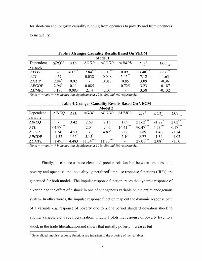
for short-run and long-run causality running from openness to poverty and from openness
to inequality.
Table 3:Granger Causality Results Based On VECM Model 1
Dependent variable
POVΔ TLΔ GDPΔ PGDPΔ UMPLΔ 2χ∑ 1−tECT
POVΔ - 4.13** 12.84*** 13.07*** 0.091 13.48*** 2.87*** TLΔ 0.57 - 0.038 0.048 5.45** 7.12 -1.63 GDPΔ 2.84* 0.02 - 0.017 0.85 3.09 -0.36 PGDPΔ 2.96* 0.11 0.085 - 0.725 3.23 -0.187 UMPLΔ 0.190 0.083 2.14 2.07 - 3.58 -0.132
Note: *, ** and *** indicates that significance at 10 %, 5% and 1% respectively.
Table 4:Granger Causality Results Based On VECM Model 2
Dependent variable
INEQΔ TLΔ GDPΔ PGDPΔ UMPLΔ
2χ∑ 1−t
ECT 1−t
ECT
INEQΔ - 3.42 2.68 2.15 1.09 21.62*** -1.77* 2.02** TLΔ 64.97*** - 2.04 2.05 16.41*** 90.47*** 4.53*** -6.17*** GDPΔ 1.342 4.53 - 4.82* 2.06 7.89 1.46 -1.14 PGDPΔ 1.52 4.62* 5.15* - 2.10 8.77 1.34 -1.02 UMPLΔ 1.495 4.483 11.34*** 11.70*** - 27.01*** 2.08** -1.50
Note: *, ** and *** indicates that significance at 10 %, 5% and 1% respectively.
Finally, to capture a more clear and precise relationship between openness and
poverty and openness and inequality, generalized2 impulse response functions (IRFs) are
generated for both models. The impulse response function traces the dynamic response of
a variable to the effect of a shock in one of endogenous variable on the entire endogenous
system. In other words, the impulse response function map out the dynamic response path
of a variable e.g. response of poverty due to a one period standard deviation shock to
another variable e.g. trade liberalization. Figure 1 plots the response of poverty level to a
shock in the trade liberalization and shows that initially poverty increases but 2 Generalized impulse response functions are invariant to the ordering of the variables.

13
Figure: 1
-.006
-.004
-.002
.000
.002
.004
.006
.008
1 2 3 4 5 6 7 8 9 10
Years
Response of Poverty to Generalized OneS.D. TL Innovation
Figure: 2
.001
.002
.003
.004
.005
.006
1 2 3 4 5 6 7 8 9 10
Years
Response of Inequality to Generalized OneS.D. TL Innovation
after two years it starts to decline. This result is consistent with trickle-down theory. In
general, the result of impulse response analysis suggests that impact of trade
liberalization on poverty is negative in the long-run. These results are similar to ones
obtained using the TYDL approach reported in the next sub-section.. Figure 2 shows that
the impact of trade liberalization on inequality is positive in the short-run but after five

14
years the impact turns negative. The above finding is similar to results reported in
Siddiqui and Kemal (2002) wherein increase in inequality is found to be the greatest at
around four years but tends to diminish in the long-run in the era of liberalization.
Granger Causality Results: TYDL Approach
The result of five variable VAR model estimated using SUR regression technique
are presented in Table 5. This outcome of Granger causality is based on TYDL
augmented lag method. These models are estimated with lag length of 3. Results from
Model 1 show that TL Granger causes POV and is significant at 5% level Furthermore,
existence of a negative relationship running from TL to POV can be deduced from the
sum of the lagged coefficients (coeff
∑ ) of the TL in the POV equation, which has a
negative sign. The results support the study of Din (2005) in which PGDP and TL has a
positive impact on poverty reduction in Pakistan. There is unidirectional causality
between TL and GDP, in which TL Granger causes GDP at 10 percent level of
significance.

15
But TL is negatively associated with GDP, i.e. more trade openness is not beneficial for
economy as it adversely affects the growth of economy. Although GDP does not cause
TL it is in negatively related with TL. This outcome may occur due to the inconsistencies
in policy formation and implementation. Another possibility for the observed negative
relationship could that the above model, given that is estimated with short lags, might not
Table 5 : Estimates of Granger Causality Based on TYDL
Model 1 Sources of Causation
POV TL GDP PGDP UMPL Dependent variables )2(2χ coeff∑ )2(2χ coeff
∑ )2(2χ coeff∑ )2(2χ coeff
∑
)2(2χ coeff∑
POV - - 10.49** -0.22 16.33*** 0.13 17.23*** -0.20 11.23** -0.37 TL 43.61*** -0.50 - - 4.58 -0.05 5.19 0.17 15.68*** -0.42 GDP 6.70* 0.04 7.23* -0.24 - - 19.14*** -1.51 2.29 -0.06 PGDP 6.47* 0.06 7.46* -0.19 17.98*** 0.67 - - 2.32 -0.04 UMPL 26.02*** 0.09 9.61** -0.07 18.49*** 0.16 14.36*** -0.22 - - Note: *, **and *** indicates that significance at 10 %, 5% and 1% respectively.
Model 2 Sources of Causation
INEQ TL GDP PGDP UMPL Dependent variables
)2(2χ coeff∑
)2(2χ coeff
∑ )2(2χ coeff∑ )2(2χ coeff
∑
)2(2χ coeff∑
INEQ - - 11.14** 0.08 6.99* -0.04 6.82* 0.09 2.50 0.06 TL 11.29** 1.30 - - 1.26 -0.08 2.17 0.26 15.50*** -2.54 GDP 19.01*** 0.34 24.26*** -1.19 - - 39.53*** -2.40 14.49*** -1.75 PGDP 20.06*** 0.16 24.30*** -1.09 37.31*** 1.192 - - 14.96*** -1.45 UMPL 41.31*** 0.498 20.65*** -0.22 17.72*** 0.160 17.11*** -0.28 - - Note: *, ** and *** indicates that significance at 10 %, 5% and 1% respectively.

16
be able to capture precise relationship between TL and GDP, especially given the fact
that as a country begins to opens up its economy it faces international competition in
initial years. However, this result is in line with Khasnobis and Bari (2000) who found
that open trade regimes do not support growth. In GDP equation the impact of
unemployment on GDP has expected sign but it is insignificant. Unemployment
coefficient has the expected sign in PGDP equation but it is also insignificant.
In PGDP equation, TL is significant at 10 percent level of significance but with an
unexpected negative sign. As tariff reduction on imports reduce the import prices and
consumer get benefit due to availability of cheap consumer goods their real income
increases. But in case of Pakistan composition of imports has not changed much in spite
of trade liberalization and tariff rates have not come down, so mostly imported products
remained expensive, which increased the price level and could have led to decline in real
PGDP.
In the unemployment equation, trade liberalization has positive influence on
unemployment level in the economy. Unemployment level has fallen due to trade
liberalization in Pakistan and level of unemployment is significant at 5 percent level. The
study of Siddiqui and Kemal (2002) depicts that after trade liberalization employment
and output show positive performance in export sector. The increase in export generates
more demand not only for imported raw material but also for labor force. As a result
unemployment level reduces for the economy. Also PGDP Granger causes
unemployment, which is significant at 1 percent level. This is theoretically sound as
increases in PGDP can reflect reduction for the unemployment level from the economy.

17
The results of Model 2 are shown in Table 5. The results show that TL has a
positive influence in Granger sense on the extent of inequality in Pakistan. It is likely that
observed positive relationship could be due to reallocation of resources on account of
trade liberalization which change factor rewards and their distribution. Due to increased
demand for capital, distribution of income becomes more skewed towards capital factor.
According to the study of Siddiqui and Kemal (2002) the degree of inequality has
increased in Pakistan in the era of liberalization. GDP negatively Granger causes
inequality at 10 percent level of significance. PGDP positively Granger causes inequality
at 10 percent level of significance. The above result could be due to the fact that there can
be more variation in the income of higher income groups as compared to middle-income
groups. Other results of model are similar to Model 1 except that in GDP and PGDP
equations, unemployment appears to be significant at 1 percent level of significance with
GDP and PGDP, both having expected signs.
V. Conclusion
Trade has always been considered a vital engine of growth and development of a
poor country may depend upon its securing adequate trade expansion. According to UN
(2004) report most LDCs undertook deep trade liberalization in the 1990s. They also
received some degree of preferential market access from developed and developing
countries. But trade liberalization plus enhanced market access does not necessarily equal
poverty reduction. Many LDCs are in the paradoxical situation that they are the ones
needing the multilateral trading system the most, but they find it hardest to derive
benefits from the application of its central general systemic principles: liberalization and
equal treatment for all its members.

18
The objective of this paper was to analyze the relationship between economic
globalization, poverty and income inequality in Pakistan. The empirical work is based on
the Granger causality testing. In this study economic globalization is found to negatively
impact poverty in the long-run by employing TYDL approach and this result is further
corroborated by the impulse response functions. The estimates from VECM show that
there exists a short-run as well as long-run relationship between trade liberalization and
poverty. Estimates from TYDL and IRFs show an adverse impact of globalization on
inequality. Overall, the study shows that globalization reduces poverty in the long-run,
generates employment opportunities but worsens inequality. It is purported that trade
liberalization aspect of globalization is a necessary but not sufficient condition for
growth. There are other mediating factors which affect the growth of the economy
ranging from political and institutional framework to historical trend in macroeconomic
variables included but not limited to population, inflation, investment and government
spending dynamics.
In short, globalization is a contested concept. However, in general it is considered
to be beneficial for the growth of economy. But there are also many adverse effects of
globalization on growth in many developing countries. It increases poverty and worsens
the income distribution. On the other hand, positive impacts of globalization have been
witnessed in East Asian Countries. These countries integrated with the world economy
within a carefully planned framework that was consistent with resource endowment, and
as a result economic rewards were shared by the poor in the long-run. It seems that the
extent of benefits reaped from economic globalization in any economy depend upon

19
domestic macroeconomic policies, market structure, initial condition of economy, quality
of institution and degree of political stability.
Lastly, it is contended that if Pakistan wants to reap maximum benefit from fruits
of economic globalization, it needs to be accompanied with adoption of pro-poor growth
policies which emphasize investment in human development and provide a structure for
social safety nets for the poor.

20
REFERENCES
Cuadros, A., V. Orts and M. Alguacil (2004), “Openness and Growth: Re-Examining Foreign Direct Investment, Trade and Output Linkages in Latin America”, Journal of Development Studies, Vol. 40(1), pp. 53-68. Din M. (2005), “Trade Policy And Poverty Experience From South Asian Region”, Paper Presented at the Annual Global Development Network Conference at Dakar, Senegal. Doloda, J.J and H. Lutkepohl (1996), “Making Wald Tests Work for Cointegrated VAR Systems”, Econometric Reviews, Vol. 15(4), pp. 369-386. Engle, R.F. and C.W.J Granger (1987), “Cointegration and Error Correction: Representation, Estimation and Testing”, Econometrica, Vol. 55, pp.251–76. Granger, C.W. J. (1988), “Some Recent Developments in a Concept of Causality”, Journal of Econometrics, Vol. 39, pp. 199-211. Granger, C.W.J. (1969), “Investigating Causal Relations by Econometric Models and Cross-Spectral Methods”, Econometrica, Vol. 37, pp. 424-438. Greenway, D., W. Morgan and P. Wright (2002), “Trade Liberalization and Growth in Developing Countries”, Journal of Development Economics, Vol. 67, pp. 229-244. Govt. of Pakistan, Economic Survey, Various Issues, Islamabad. Johansen, S. (1988), “Statistical Analysis of Cointegrating Vectors”, Journal of Economic Dynamic and Control, Vol. 12, pp. 231-254. Johansen, S. and K. Juselius (1990), “Maximum Likelihood Estimation and Inference on Cointegration with Applications to the Demand for Money”, Oxford Bulletin of Economics and Statistics, Vol. 52, pp. 169-210. Kemal, A.R., M. Din and U. Qadir (2002), “Global Research Project: Pakistan Country Report”, Pakistan Institute of Development Economics, Islamabad. Khasnobis B.G. and F. Bari (2000), “Sources of Growth in South Asian Countries”, Global Research Project of the World Bank. Rambaldi, A. and H. Doarn (1996), “Testing for Granger Non-Causality in Cointegrated Systems Made Easy”, Working Papers in Econometrics and Applied Statistics No.88, The Department of Econometrics, University of New England.
21
Round J. and J. Whalley (2002), “Globalization and Poverty: Implications of South Asian Experience for Wider Debate”, DFID (Department of International Development) Project Paper. Siddiqui R. and A.R.Kemal (2002), “Remittances, Trade Liberalization, and Poverty in Pakistan: The Role of Excluded Variables in Poverty Change Analysis”, DFID Project Paper. Toda, H.Y. and P.C.B Phillips (1993) “Vector Autoregression and Causality”, Econometrica, Vol. 61, pp. 1367-1393. Toda, H. Y., Phillips, P. C. B. (1994), “Vector Autoregression and Causality: A Theoretical Overview and Simulation Study”, Econometric Reviews, Vol. 13, pp. 259-285. Toda, H.Y and T. Yamamoto (1995), “Statistical Inference in Vector Autoregression with Possibly Integrated Processes”, Journal of Econometrics, Vol. 66, pp.225-250. United Nations (2004), The Least Developed Countries Report, UNCTAD, New York.