Department of Applied Economics V - University of the Basque Country &

Cambridge Centre for Economic and Public Policy - University of Cambridge

6th International Conference Developments in Economic Theory &Policy, Bilbao (Spain), July 2-3, 2009

Economic Fluctuations, Cyclical

Regularities and Technological Change:

The U.S. Food Sector (1958–2006)

Theofanis Papageorgiou, Panayotis Michaelides* and John Milios

National Technical University of Athens, Greece

Abstract

Despite the fact that the U.S. food sector is a key component of U.S.

manufacturing, it has attracted limited attention in the literature, so far. In

fact, the recent food crisis shed some light on different aspects of the food

sector, its products and its influence on millions of people. The sector is

characterised by increasing concentration, changes in relative prices, shifts in

consumer preferences and changes in government regulations. However, key

issues related to technological change and the cyclical regularities of economic

time series in the sector have been neglected or even unexplored in the

literature. Our study provides robust evidence supporting the fact that

technological change has explanatory power for output and profitability in the

Granger-causal sense at various leads or lags. Also, the timing pattern of

technological change indicates that the peak correlations appear at moderate

lags. This implies that the technology shocks are transmitted in the economy

relatively quickly. Also, the various economic time series in the sector seem to

follow a cyclical pattern characterized by periodicities exhibiting a short-term

cycle, a mid-term cycle and a long-term cycle.

Keywords: profitability, output, technology, fluctuations, US food sector

* Lecturer in Economics (407/80); email: pmichael@central.ntua.gr; fax: +302107721618 (Contact Author).

2

1. Introduction

The food manufacturing sector is one of the largest in United States (U.S.)

manufacturing and in U.S. economy in general. However, it has attracted limited

attention in the literature, so far. According to the Annual Survey of Manufacturers,

around 28.000 establishments exist in the sector employing about 1.500.000 people

or 11% of the manufacturing sector and more than 1% of total U.S. economy (2006).

Meanwhile, it contributes more than 10.5% in total manufacturing output and

approximately 2% of U.S. output (2006). The food production, processing, wholesale

distribution, and retailing system are important components of the U.S. economy

accounting for 12.8 % of U.S. gross domestic product (GDP) in 2000. Furthermore,

the sector exports products accounting for about 33 billion dollars. Also, the sector is

one of high concentration, and food processing industries are among the most

profitable industries in the U.S. (Wang et al. 2006). Finally, market structure in the

industry has changed significantly over the last fifty years and is mainly the result of

mergers and acquisitions. In fact, the period 1977–1987 coincides with one of the four

U.S. merger movements.

The typical features characterizing the sector are: increased consolidation and

concentration, changes in relative prices, shifts in consumer preferences and changes

in government regulations (Adelaja et al. 1999, Morrison 1997, Rogers, 2001). It is a

capital intensive sector, where materials contribute about 60% of total output (Huang

2002), it is responsive to new technologies in processing, packaging and marketing of

food product and has become increasingly high tech over the past decades (Morrison

1997). Also, it experienced low productivity growth rates compared to other sectors

(Huang, 2002) and Total Factor Productivity (TFP) behaved cyclically (Heien 1983).

In this context, there are several reasons for studying the U.S. food

manufacturing sector: first, there are limited studies on topics such as economic

fluctuations and crises at the sectoral level; second, it is a very important sector for

the U.S. economy; third, the recent food crisis shed some light on different aspects of

the food sector, its products and its influence on millions of people; fourth, the

impact of the current crisis on the food manufacturing sector is of great interest

taking into account its high income inelasticity. At first, the food manufacturing

sector did not seem to be seriously affected by the recent economic crisis because of

the high income inelasticity of food products. However, no doubt a closer look would

be of great interest. After all, judging from previous crises, and knowing that

profitability practically collapses during or after the crisis period (e.g. Dumenil and

Lévy, 2002; Wolff 2003; Mohun, 2005), it is quite reasonable to expect a downward

trend in profitability.

3

This paper investigates how technological change affects indicators of economic

and social welfare, such as profitability and output in the US food manufacturing

sector, in the time period 1958-2006. We begin by analysing the stylised facts of the

fundamentals in the food manufacturing sector for the time period 1958-2006. In

order to investigate the stationarity properties of each time series we test the existence

of unit roots. Given that the economic series usually contain a trend, de-trending is

highly recommended. Moreover, we use spectral analysis to extract periodograms

which indicate the lengths of the business cycle based on the available data and then

we test whether the various de-trended economic time series tend to follow a cyclical

pattern, or their evolution is white noise. Next, we focus on answering some

fundamental economic questions regarding the interpretation of the cyclical

behaviour of underlying economic variables in the sector. For instance, how does

technology affect the behaviour of variables, such as real output and profitability

over time?

The paper is organized as follows: section 2 offers a brief review of the literature

on the U.S. food manufacturing sector; section 3 sets out the methodology; section 4

presents and discusses the empirical results; finally, section 5 concludes the paper.

2. Review of the Literature

Supply oriented shock models dominate studies in the food manufacturing

sector; TFP, productivity and market structure studies are among them. As we know,

TFP growth is, among other things, typically used as a proxy for technological change

(Morisson 1992). Some studies on TFP growth use the conventional method of

growth accounting, defined as the rate of aggregate output minus the rate of growth

of aggregate inputs. This method usually assumes constant returns to scale and

perfect competition.

Heien (1983) was probably the first who tried to measure productivity in the

food manufacturing sector. The paper measured TFP using Theil–Törnqvist indexes

of total outputs and total inputs, finding evidence of cyclical behaviour. Furthermore,

the paper provided an explanation for the decrease in TFP in the time period 1973 –

1977 as the result of (a) an increase in energy costs, (b) the stricter government

regulation, (c) the erratic money and fiscal policy, and (d) the demographic changes

in labour force.

Huang (2002) measured TFP and labour productivity growth in the time period

1975 – 1997. The paper concluded that an important characteristic of the sector is its

weak TFP growth compared to other sectors of U.S. manufacturing, and this, the

paper argues, is due to the low investment rate in R&D. As a result, the slow growth

4

in productivity signifies (a) the expansion of combined factor inputs to food

manufacturing output instead of productivity growth; (b) a limited contribution on

price declines in food products in recent years, which is attributed to cheaper input

prices.

Gopinath and Carver (2002) used data for thirteen (13) countries to examine

the effects of productivity growth in agriculture on the processed food sector. One of

their findings is that U.S. has the lowest food TFP growth level among the countries

investigated with the exception of Japan. Finally, they argued that public policies

protecting primary agriculture can adversely affect processed food sectors, while

those supporting Research and Development (R&D) efforts can bring about dynamic

comparative advantage.

According to Azzam et al. (2002) the most important source of TFP growth in

the food industry was demand growth, whereas the most important negative

contributor to TFP growth was disembodied technological change. Also, Hossain et

al. (2005) argued that the use of debt financing increased sharply resulting in

changes either in productivity or performance, while increased debt use reduced

productivity growth.

Morrison and Siegel (1997) investigated whether technological change and

international competitiveness are responsible for the observed changes in

productivity and input composition in the U.S. food manufacturing sector. The study

suggested that the cost reduction was the result of increased competitiveness (trade)

and knowledge capital (general technological advance or automation).

Morrison (1999) examined the impact of capital investment and import

penetration on firms’ costs and prices. The analysis concluded that the increased cost

efficiency arises from reduced labour use. In fact, scale economies and increased high

– tech capital are labour saving, energy and materials using.

In a recent study, Geylani and Stefanou (2008) examined the relationship

between productivity and investment spikes for the food manufacturing industry in

the 1972-1995 time span. Their key results may be summarized as follows: first, there

is a significant variation in productivity growth; second, the learning period

associated with investment spikes differs among quartile groups; third, there is a

decreasing probability of an investment spike as the time since the last spike

increases.

Galo (1992) found that aggregate profitability of the sector, when measured as a

return on the assets and stockholders’ equity, is one of the highest in manufacturing.

However, aggregate profitability on sales for food manufacturing is below the average

for nondurable manufacturing because of a high sales turnover rate.

5

Finally, market structure has attracted increasing attention among researchers

in the field (e.g. Röder et al. 1999). For instance, Goodwin and Brester (1995) found

that the structural changes in the sector resulted in the following: (a) the demand for

raw food materials and energy became more elastic; (b) the demand for labour

became less elastic; (c) nearly all input factors can be regarded as substitutes, and (d)

the degree of the substitutability has significantly increased in recent years, due to

technical change. In a similar vein, Röder et al. (1999) found a typical U – type effect

of concentration on innovations and the number of firms. Additionally, the degree of

existing product differentiation and the market size positively affected the number of

innovations. Finally, in a recent study Wang et al. (2006) analysed the relationship

between market concentration and other variables and one of their main findings was

the increasing significance of the role of high - tech capital and the changes in

production technology.

To sum up, there are several studies that make an attempt to link productivity

growth in the U.S. food manufacturing sector to some key variables. Most of them

focus on technological change, while others emphasise on market structure.

However, no study, to the best of our knowledge, deals with the questions of

instability and crisis and the role of technological change.

3. Methodology According to this section, which is based on Michaelides et al. (2007), the business

cycle component is regarded as the movement in the time series that exhibits

periodicity within a certain range of time duration. This approach is often called the

“classical business cycles” approach and is based on Burns and Mitchell (1946) and

the National Bureau of Economic Research (NBER). This approach argues that

business cycles are characterized by the “turning point” which indicates, roughly

speaking, the beginning of an expansionary period at the end of a recession. Another

popular approach regards business cycles as fluctuations around a trend, the so-

called “deviation cycles” (Lucas 1997). The estimation of this trend for each time

series is of great importance because it is necessary for the extraction of the cyclical

component. In this study we adopt both these approaches.

6

First, we examine the stationarity characteristics of each time series. As we

know there are several ways to test for the existence of a unit root. In this paper, we

use the Augmented Dickey – Fuller methodology (ADF) (Dickey and Fuller, 1979).1

If the results suggest that the time series are stationary in their first

differences then, de-trending is highly suggested.

The ADF test is based on the following regression (Kaskarelis 1993):

t

m

iititt YYbta ε+Δγ+ρ++=ΔΥ ∑

=−−

11 (1)

where Δ is the first difference operator, t is time and ε t is the error term.

(a) If b≠0 and ρ=-1 implies a trend stationary (TS) model.

(b) If b=0 and -1<ρ<0 implies an ARMA Box/Jenkins class of models.

(c) If b=0 and ρ=0 implies a difference stationary (DS) model where Y variable is

integrated of degree one I(1). If we assume that the cyclical component is stationary,

the secular component has a unit root and Y follows a random walk process (i.e. it

revolves around the zero value in a random way (Heyman and Sobel 2004, p. 263).

Furthermore, if α≠0 Y follows a random walk process with a drift. The lag dependent

polynomial is inserted in order to deal with the potential serial correlation of the

residuals.

The trend is important for the propagation of shocks (Nelson and Plosser

1982). Linear, exponential and quadratic de-trending is highly recommended and the

estimated residuals constitute the de-trended data series.

A time series tx with a linear deterministic trend is as follows:

t tx a bt ε= + + (2)

where a and b are parameters, t is time and ε t is white noise.

A time series tx with an exponential deterministic trend is as follows:

log t tx a bt ε= + + (3)

where a , b are parameters, t is time and tε is white noise.

A time series tx with a quadratic deterministic trend is as follows:

2t tx a bt ct ε= + + + (4)

where a , b, c are parameters, t is time and tε is white noise.

Besides these methods we also use the following, widely used, alternative approaches:

1 Alternatively, the test of Zivot and Andrews (1992) could have been used or some other unit root tests such as the IPS test (Im et al. 1997), the MW test (Maddala and Wu 1999), or the Choi test (Choi, 2001).

7

(a) The Hodrick-Prescott Filter

The linear, two-sided HP-filter approach is a widely used method by which the long-

term trend of a series is obtained using only actual data. The trend is obtained by

minimizing the fluctuations of the actual data around it, i.e. by minimizing the

following function:

( ) ( ) ( ) ( ) ( ) ( )22

ln ln * ln * 1 ln * ln * ln * 1y t y t y t y t y t y tλ ⎡ ⎤− − + − − − −⎡ ⎤ ⎡ ⎤ ⎡ ⎤⎣ ⎦ ⎣ ⎦ ⎣ ⎦⎣ ⎦∑ ∑ (5)

where y* is the long-term trend of the variable y and the coefficient λ>0 determines

the smoothness of the long-term trend.

This method decomposes a series into a trend and a cyclical component. The

parameter used for annual data is equal to λ=100 (Hodrick and Prescott 1997,

Kydland and Prescott 1990, Canova 1998).

A large number of studies has used the HP filter de-trending method for

different purposes (e.g. Danthine and Girardin 1989, Blackburn and Ravn 1992,

Backus and Kehoe 1992, Fiorito and Kollintzas 1994). The Hodrick and Prescott

Filter is able to extract the same trend from all time-series which is considered a

significant advantage since many real business cycle models indicate that all variables

will have the same trend.2

(b) The Baxter-King Filter

Another popular method for extracting the business cycle component of

macroeconomic time series is the Baxter-King Filter (Baxter and King 1999). The

Baxter King filter is based on the idea to construct a band-pass linear-filter that

extracts a frequency range [ ]min max,ω ω dictated by economic reasoning. Here, this

range corresponds to the minimum and maximum frequency of the business cycle.

The algorithm consists in constructing two low-pass filters, the first passing

through the frequency range [ ]max0,ω (denoted as ( )a L , where L is the lag operator)

and the second through the range [ ]min0,ω (denoted as ( )a L ). Subtracting these two

filters, the ideal frequency response is obtained and the de-trended time series is:

( ) [ ] ( )BPy t a a y t= − (6)

Two of the main advantages of this approach are: first, it leaves the properties

of the extracted component unaffected and, secondly, it does not change the timing of

the “turning points”. There is widespread agreement that a business cycle lasts

2 However, there are shortcomings as well in this approach. For overviews of the HP filtering method shortcomings see Harvey and Jaeger (1993), King and Rebelo (1993), Cogley and Nason (1995) and Billmeier (2004).

8

between 8 and 32 quarters and the length of the (moving) average is 12 quarters

(Baxter and King 1999). This is due to the seminal works of Burns and Mitchell

(1946).3 Consequently, these are the values (2 to 8 years) that we use in the de-

trending methods described above.

A large number of studies have used the Baxter-King filtering method (see e.g.

Stock and Watson 1999, Wynne and Koo 2000, Agresti and Mojon 2001, Benetti

2001, Massmann and Mitchell 2004).

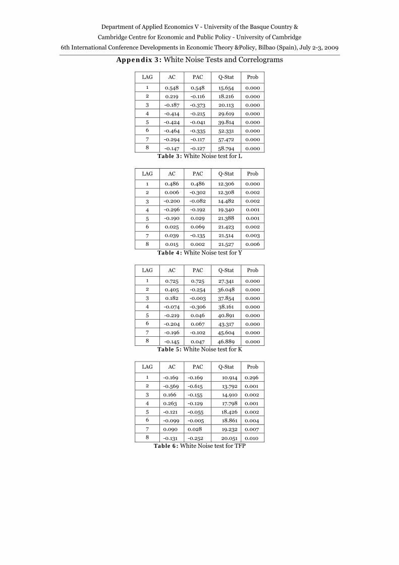
As it is well-known, white noise does not permit any temporal dependence4

and so its autocovariance function is trivially equal to zero for the various lags. The

sample autocorrelation function measures how a time series is correlated with its

own past history. Its graphical illustration is the correlogram. In order to test for

autocorrelation we use the Ljung and Box (1978) test (Q-stat) which practically tests

the null hypothesis of white noise for a maximum lag length k. The alternative

hypothesis is that at least one of theses autocorrelations is nonzero, so that the series

is not white noise. In case the null hypothesis is rejected then the underlying time

series is clearly not white noise and can be considered a cycle. In case we are dealing

with a trending time series, then we study and test not the raw series but its

deviations from trend, i.e. the residuals from which sample autocorrelations can be

computed.

Here we investigate the periodicities of business cycles assuming that the

actual fluctuations of the data are chiefly of a periodic character. We are supposing

that the presence of periodic elements in the given fluctuations is possible. It is the

object of this section to isolate those elements and indicate the approximate length of

the cycle. The length of the period in an economic series may, in general, be variable.

Therefore, we understand by the term “period” the average length of the cycles and

the periodogram can assist in finding these average lengths.

The period is measured by constructing a graphical illustration of the value R

in the time frequency and checking for the highest pick:

R i =22

ii ba + , ∑=

π=αn

tti itX

n 1)/2cos(2, )/2sin(2

1itX

nb

n

tti π= ∑

=

, 1,2,...i m= , / 2m n= (7)

where ia , ib are the coefficients of the Fourier-transformed function tX (Rudin 1976).

Next, we investigate whether technological change has predictive power for

profitability and output growth, respectively, in the Granger-causal sense. Thus, we

conduct bi-variate (Granger) causality tests between:

3 For a critique to this approach see Agresti and Mojon (2001). 4 Actually, white noise is a data generating process where autocorrelation is zero between lagged versions of the signal (except when the lag is zero).

9

(a) Technological change (TFP) and real output (GDP)

(b) Technological change (R&D) and real output (GDP)

(c) Technological change (TFP) and Profitability (Profit Rate)

(d) Technological change (R&D) and Profitability (Profit Rate)

(e) Technological change (Labour Productivity) and Profitability (Profit Rate)

No doubt, profitability is the cornerstone of economic theory in a capitalist

economy. A relevant measure that is convenient because it expresses profitability as

a percentage rate is the so-called rate of profit which expresses the rate of return on

capital invested (Moseley 2003, and Zachariah 2009).

Meanwhile, technology constitutes a very crucial determinant of sectoral

competitiveness. A major problem in examining technological change and one that

makes it difficult to define or characterize it is that it can take many different forms

(Rosenberg, 1982: 3). In that sense, there is no generally accepted measure of

technological change and all measures are imperfect, so, we decided to use three of

them to quantify technological change. TFP is based upon strong assumptions and

approximates technological change as the residual of the growth equation. As a result

this measure could lead to misleading interpretations of technology. Alternatively, it

is widely argued that there is convincing evidence that cumulative R&D is an

important determinant of technology. Finally, several theoreticians, usually Marxists,

argue that labour productivity expresses, in a nut-shell, technology as a productive

force.

The concept of causality, introduced by Granger (1969) has been widely used

in economics. In general, we say that a variable X causes another variable Y if past

changes in X help to explain current change in Y with past changes in Y. Thus, the

empirical investigation of (Granger) causality is based on the following general

autoregressive model (Karasawoglou and Katrakilidis 1993):

(8)

where Δ is the first difference operator, ΔY and ΔX are stationary time series and tε is

the white noise error term with zero mean and constant variance.

The null hypothesis that X does not Granger-cause Y is rejected if the

coefficient ia2 is statistically significant. Various lag-lengths are tested in order to

identify the optimal value. The optimal lag could be selected using one of the

following criteria: (a) FPE (final prediction error), (b) AIC (Akaike information

criterion) and (c) Hannan – Quinn information criterion.

0 1 21 0

m n

t i t i i t i ti i

a a Y a X ε− −= =

ΔΥ = + Δ + Δ +∑ ∑

10

The most frequently used testable hypotheses are expressed as follows: (a) Y

Granger-causes X, (b) X Granger-causes Y (c) Y and Granger cause each other, and

(d) neither variable Granger–causes the other.

4. Empirical Investigation We implement the aforementioned techniques in order to investigate empirically the

cyclical behaviour of relevant economic time series in the U.S. food manufacturing

sector. The data used are on an annual basis and come from the National Bureau of

Economic Research (NBER) database and from the U.S. Census Bureau, Department

of Manufacturers and cover the period 1958-2006, just before the first signs of the

global economic recession made their appearance. The data on capital stock stopped

in 1996, and we estimated the rest of the time series based on the popular

methodology employed in Huang (2002).

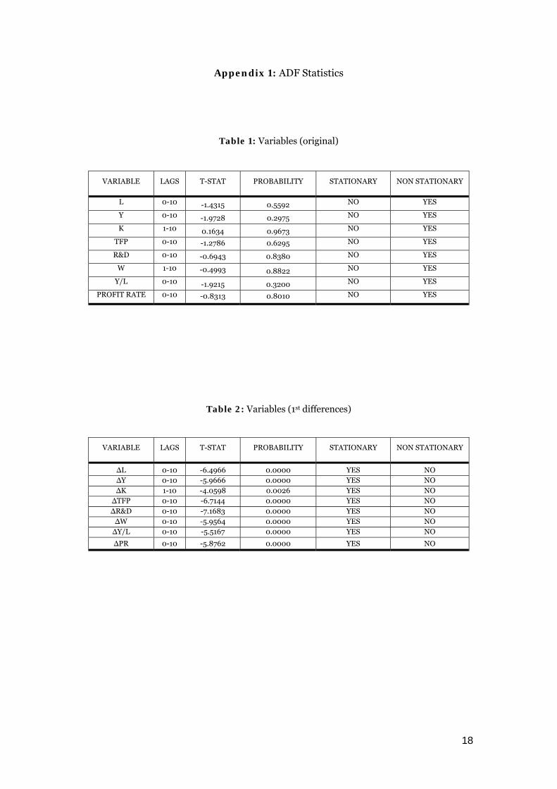
To begin with, the stationarity properties of the various macroeconomic

variables were checked. Table 1 shows the results of the Augmented Dickey-Fuller

test regarding the following time series : labour (L) i.e. number of employees, real

output (Y) i.e. output in dollars at constant prices, stock of fixed capital (K) i.e. in

dollars, total factor productivity (TFP) i.e. in percentage change, real wages (W) i.e.

total amount of wages to L in dollars, labour productivity ( /Y L ), research and

development (R&D) expenditures, i.e. in dollars and the profit rate (Π), defined as

percentage rate: Π=Y W

K−

(Duménil and Lévy 2004).

All macroeconomic variables are non-stationary, however their first

differences are stationary (Table 2). The next step was to de-trend the variables.

Various de-trending approaches were employed and the graphs of the residuals are

depicted in Fig. 1. Also, the results of the analysis based on the correlograms for the

various economic time series are shown in Tables 3-10. The results of the Ljung/Box

test indicate a rejection of the null hypothesis of white noise for all the de-trended

variables under investigation. In other words, the existence of cyclical regularities is a

valid hypothesis from a statistical viewpoint.

The periodograms reveal the periodicity of the cycles and are shown in Figs.

2-9. The de-trended real output seems to follow a short-term (1 year), two mid-term

(3 and 5 years) and one long-term cycle (7 years) (Fig. 3). The spectral content of the

cyclical component of R&D (Fig. 5) exhibits local maxima at the frequencies of 3, 5

and 7 years. Accordingly, the de-trended labour productivity is characterized by the

same frequency peaks (Fig. 8) (1, 3 and 7 years) giving credit to the belief that the

11

cyclical movements of R&D and labour productivity seem to be synchronized, at least

to a great extent. Also, the cycle of the profit rate is characterized by periodicities of 1,

3 and 7 years. Finally, an interesting observation is that most economic time series

exhibit, roughly speaking, a similar pattern characterized by periodicities exhibiting a

short term cycle (approximately 1 year), a mid-term cycle (approximately 3 years)

and a long term cycle (approximately 7 years), same as the periodisation of output.

These results can be interpreted by economic theory as indications for the existence

of cycles with different lengths (i.e. periods) that are also synchronized for the

different variables within the total economy.

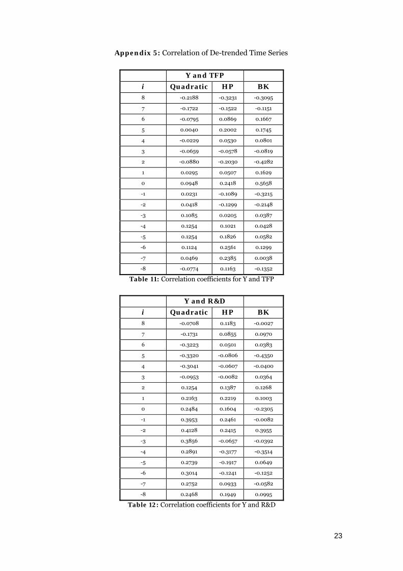
Tables 11-15 show the correlation coefficients between the variables under

discussion. It can be seen that in all cases peaks occur at moderate lags (and leads)

implying a relatively rapid transmission process of technological shocks throughout

the food manufacturing industry.

Table 16 presents the results of the Granger causality tests. As can be inferred,

the profit rate seems to be caused (in the Granger sense of the term) by TFP, R&D

and labour productivity, while TFP and R&D cause, independently, real output.

Our findings are consistent with the majority of studies in the relevant

literature. For instance, the cyclical behaviour of certain key variables such as profit

rate and total factor productivity is consistent with the findings by other researchers

(e.g. Heien 1983; Galo 1992). Also, according to our findings technological change

goes hand in hand with output and profitability as (e.g. Goodwin and Brester, 1995;

Morrison, 1999; Morrison and Siegel, 1997).

5. Result Analysis and Discussion

To begin with, from a mere visual inspection, we note that output fluctuations

in the US food manufacturing sector are not very sharp although trends, upswings

and falls do exist (Fig. 1a). Also, one can infer that the output of the U.S. food

manufacturing sector seems to behave in a way analogous to U.S. GDP (Bureau of

Economic Analysis, U.S. Department of Commerce). Analytically, the collapse of

output following the first “oil crisis” is common in the U.S. food manufacturing sector

and the US economy in total. Between 1963 and 1972, there is a clear upward trend in

the output of the industry that was stopped by the “oil crisis”, the effect of which is

evident in the de-trended time series irrespectively of the filter used. Furthermore,

the cyclical component follows the same pattern both in the economy and the sector

between 1979-1982 and 1990-1991. The 1990’s began with a shallow recession (Basu

et al., 2001) and, according to the economic report of the President (1994), the speed

12

of recovery was very slow5. Furthermore, between 1991 and 1997 – the so-called “new

economy” period – a sharp increase of output took place. Also, productivity growth in

the sector coincided with an exceptionally good performance of the U.S. economy

(Mankiw, 2001)6. Of course, differences exist with respect to the magnitude of the

fluctuations. Attempting to decompose fluctuations in industrial output, the possible

sources seem to be aggregate (national) shocks, industry group specific shocks and

idiosyncratic factors (Norrbin and Schlagenhauf, 1990).

Regarding the de-trendeded profit rate (figure 1h) it reached its highest level

in 1972 and then it was affected by the negative macroeconomic environment of the

1970’s and chiefly the oil crisis. This period is often documented as the second period

of great decrease in the U.S. profit rate after WWII. Finally, an upward movement

occurred in the beginning of the 1980’s until 1986 reaching its peak in 1988 and 1997.

This rise coincides with the third period of the U.S. economy characterised by a

period when profitability rose as a result of the rapid rise in the productivity of

labour.7

As for the labour force, during the 1970s and 1980s a structural change

occurred, when huge numbers of workers entered the U.S. labour force: baby

boomers, women, immigrants, etc. The American economy gave jobs to all of them.

Unemployment peaked during the lowest point of the business cycle, 1982 – 1983,

reaching a high 10.8%. At the same time, there was an obvious trend of diminishing

the number of employees in the food manufacturing industry beginning in the 1980-

1986 time span (fig. 1c). The principal constraint on reducing unemployment was the

fear of the Federal Reserve that too low an unemployment rate would lead to

accelerating inflation. However, after 1983 there was a gradual decline in the

unemployment rate reaching a minimum in 1989, a fact that is reflected in the

increase of employment in the industry. This could be attributed to the introduction

of flexible forms of labour, as a result of the Reagan economic policies, that reduced

the official unemployment records. Finally, a slight increase in the number of

unemployed took place right after the terrorist attacks of September 2001, which is

depicted in the sectors’ employment.

The value of labour power has a downward trend falling continuously from

1978 onwards (Mohun 2005). Wages are squeezed on profits from the mid 1960’s to

5 The speed of recovery was very slow both for output and labor, between the peak in the second quarter of 1990 and the trough of the first quarter of 1991. See Economic Report for the President (1991). 6 Mankiw (2001) argued that the macroeconomic performance of the 1990’s was exceptional, food and energy prices were well behaved and productivity growth experienced an unexpected acceleration, i.e. the so-called “new economy” which was characterized by the increasing role of I.T. 7 Most economists define 3 broad periods in the U.S. economy after WWII. According to Wolff (2003), these are: (a) 1947-1966, (b) 1966-1979 and (c) 1979-1997, the first as a period of rising profitability, the second as a decreasing one and the third as a recovery one.

13

the early 1980’s and the wage share rose some 10% of money value added. The

cyclical component of wages (fig. 1g) has its peak in 1978 and its lowest point in 1997.

Between 1981 and 1987 de-trended wages remained at low levels a fact that may be

related to Reagan’s program for steady wages. After 1997, there is an upward trend.

Fig. 1b shows the fluctuations of the net capital stock invested in the U.S. food

manufacturing. According to Basu et al. (2001) the 1990’s experienced a boom in

business investment of unprecedented size and duration. The 1970’s was a decade

characterized by an investment boom (just like the 1990’s) but less prolonged.

Furthermore, the authors showed that a large part of that increase was due to

investment in information technology (I.T.) equipment (computers plus

communications equipment). Our findings follow the same patterns as the cyclical

components described earlier. Finally, a clear decreasing pattern is evident after

2001, which may be related to the IT technology bubble and the terrorist attacks of

2001.

Meanwhile, TFP quantifies the evolution of technological change (fig. 1d). The

TFP time series stops in 1996 due to data availability (NBER). Except for TFP, R&D

expenditures are also used in order to quantify technological change (fig. 1e). The

cyclical component of TFP in the food manufacturing has two obvious trends one

downward from 1973 to 1980 and one upward from 1981 to 1988. Between 1948 and

1973 TFP grew annually in the US by 2.13% one of the highest growth rates ever

recorded in U.S. history. Also, U.S. net investment grew substantially in the 1950’s

and the 1960’s as U.S. corporations went multinational (Krugman 1990). This

increase may be a reason for the high increase of TFP. After the “oil crisis” of 1973,

the rate went down to 0.53% per year for the years 1973 – 1989. After 1989 there is a

gradual increase going to 0.93% per year until 2000 and to 1.83% for 2000 -2005.

Also, the “oil crisis” caused the contraction of R&D expenditures until 1983. The tax

cut policy introduced by the Reagan government pushed profitability upwards and

gave motives for investment. The increase in the U.S. food sector R&D expenditures

might be related to this policy.

Labour productivity was more or less steady from 1958 to 1970 and increased

until 1973, whereas the 1973 shock put an end to this upward trend (fig. 1f). After

1974, fluctuations were more acute. From a visual inspection of the graphs in figs. 1g,

1e and 1f, it is obvious that the cyclical movements of labour productivity, TFP and

R&D go hand in hand, as expected. This observation is consistent with the noted

improvement in the investment performance in the food manufacturing sector and

the more high–tech nature of the sector (Morrison 1997), and, of course, the increase

in total investment in the U.S. in the 1950’s and 1960’s (Krugman, 1990).

14

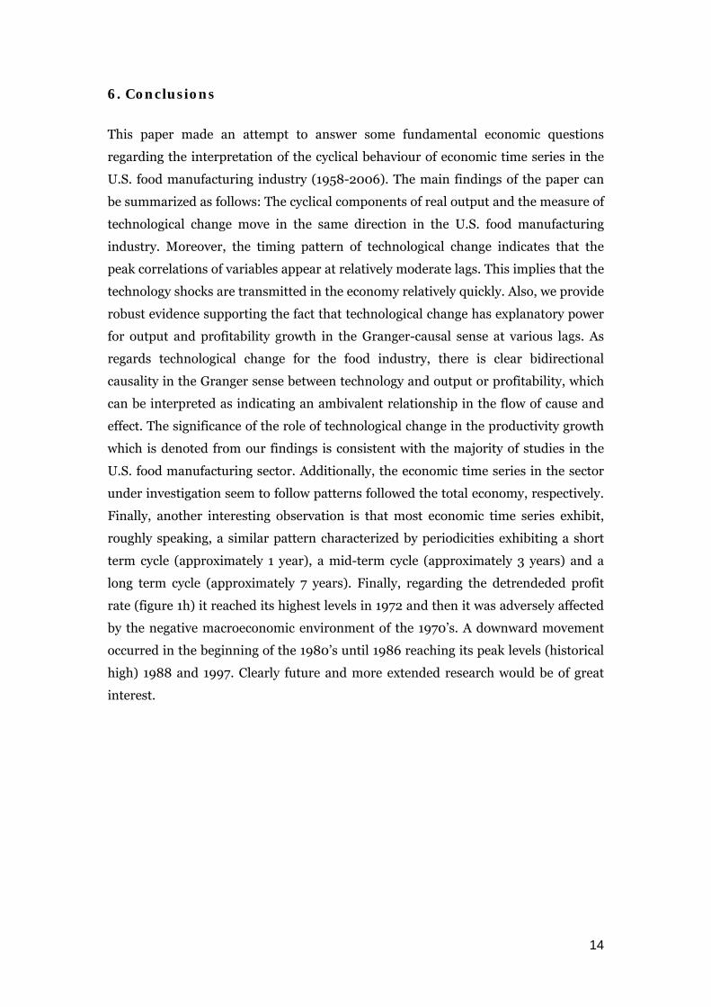
6. Conclusions

This paper made an attempt to answer some fundamental economic questions

regarding the interpretation of the cyclical behaviour of economic time series in the

U.S. food manufacturing industry (1958-2006). The main findings of the paper can

be summarized as follows: The cyclical components of real output and the measure of

technological change move in the same direction in the U.S. food manufacturing

industry. Moreover, the timing pattern of technological change indicates that the

peak correlations of variables appear at relatively moderate lags. This implies that the

technology shocks are transmitted in the economy relatively quickly. Also, we provide

robust evidence supporting the fact that technological change has explanatory power

for output and profitability growth in the Granger-causal sense at various lags. As

regards technological change for the food industry, there is clear bidirectional

causality in the Granger sense between technology and output or profitability, which

can be interpreted as indicating an ambivalent relationship in the flow of cause and

effect. The significance of the role of technological change in the productivity growth

which is denoted from our findings is consistent with the majority of studies in the

U.S. food manufacturing sector. Additionally, the economic time series in the sector

under investigation seem to follow patterns followed the total economy, respectively.

Finally, another interesting observation is that most economic time series exhibit,

roughly speaking, a similar pattern characterized by periodicities exhibiting a short

term cycle (approximately 1 year), a mid-term cycle (approximately 3 years) and a

long term cycle (approximately 7 years). Finally, regarding the detrendeded profit

rate (figure 1h) it reached its highest levels in 1972 and then it was adversely affected

by the negative macroeconomic environment of the 1970’s. A downward movement

occurred in the beginning of the 1980’s until 1986 reaching its peak levels (historical

high) 1988 and 1997. Clearly future and more extended research would be of great

interest.

15

References

Adelaja A., NaygaR. Jr., Farooq Z. (1999), Predicting Mergers and Acquisitions in the Food Industry, Agribusiness 15, 1- 23. Agresti, A-M. and B. Mojon (2001), Some Stylized Facts on the Euro Area Business Cycle, ECB Working Paper 95. Artis, M., (2003), Analysis of European and UK business cycles and shocks, EMU Study for HM Treasury. Atella V., and B. Quintieri (2001) Do R&D Expenditures really matter for TFP, Applied Economics 33, pp. 1385 – 1389. Azzam A., E. Lopez and R. Lopez, (2002), Imperfect Competition and Total Factor Productivity Growth in U.S. Food Processing, Food Marketing Policy Center Research Report No. 68. Backus, D.K., and P.J. Kehoe (1992), International evidence on the historical properties on business cycles, American Economic Review, 82(4), pp. 864-888. Basu S., Fernald J. And Shapiro M., (2001), Productivity Growth in the 1990’s: Technology, Utilization or Adjustment, Carnegie – Rochester Conference Series on Public Policy 55, pp. 117 – 165. Baxter, M. and R.G. King (1999), Measuring Business Cycles: Approximate Band-pass Filters for Economic Time Series, Review of Economic and Statistics, 81(4), 575-593. Beneti, L. (2001), Band-Pass Filtering Cointegration and Business Cycle Analysis, Bank of England, Working Paper 142. Billmeier, A. (2004) Ghostbusting: which output gap measure really matters?, IMF Working paper WP/04/146. Blackburn, K., and M. Ravn (1992), Business Cycles in the United Kingdom: Facts and Frictions, Economica, 59, pp. 382-401. Burns, A.F., and W.C. Mitchell (1946), Measuring Business Cycles, New York: National Bureau of Economic Research. Choi, I. (2001), Unit Root Tests for Panel Data, Journal of International Money and Finance, 20, pp. 249-272. Coe D. T., and Helpman E., (1995), International R&D Spillovers, European Economic Review, 39, pp. 859 – 888. Cogley, T., and Nason, J.M. (1995), .Effects of the Hodrick-Prescott Filter on Trend and Difference Stationary Time Series: Implications for Business Cycles Research, Journal of Economic Dynamics and Control, 19, 253-278. CoyleW., M.Gehlhar, T. Hertel, Z. Wang and W. Yu (1998), Understanding the Determinants of Structural Change in Terms of Trade, Americal Journal of Agricultural Economics 80, pp. 1051 – 1061. Danthine, J.P., and M. Girardin (1989), .Business Cycles in Switzerland. A Comparative Study, European Economic Review, 33, pp. 31-50. Dickey, D.A. and Fuller, W. A. (1979), Distribution of the Estimates for Autoregressive Time Series With a Unit Root, Journal of the American Statistical Association, 74, pp. 427-431. Duménil G., and D. Lévy (2002), The Profit Rate: Where and How Much Did it Fall? Did it Recover? (USA 1948 – 2000) Review of Radical Political Economics 34, pp. 437 – 461 Economic Report of the President (1994) Fiorito, R., and T. Kollintzas (1994), Stylized Facts of Business Cycles in the G7 from a Real Business Cycle Perspective, European Economic Review, 38, pp. 235-269. Galo A., (1992) Aggregate Profitability in U.S. Food Manufacturing, Journal of Food Distribution Research 1992, pp. 71 – 80. Geylani P.C., Stefanou S. (2008), Linking Investment Spikes and Productivity Growth: U.S. Food Manufacturing Industry, Discussion Papers, Center of Economic Studies, Bureau of the Census.

16

Goodwin B. and Brester G. (1995), Structural Change in Factor Demand Relationships in the U.S. Food and Kindered Products Industry, Americal Journal of Agricultural Economics 77 pp. 69 -79. Gopinath M. And Carver J. (2002), Total Factor Productivity and Processed Food Trade: A Cross Country Analysis, Journal of Agricultural and Resource Economics 27, No.2, pp. 539 – 553. Granger, C. W.J. (1969), Investigating Causal Relations by Econometric Models and Cross-Spectral Methods, Econometrica 37, July, pp. 424-438. Harvey, A.C., and Jaeger, A. (1993), Detrending Stylized Facts and the Business Cycle, Journal of Applied Econometrics, 8, 231-247. Heien D. (1983), Productivity in U.S. Food Processing and Distribution, American Journal of Agricultural Economics pp. 297 – 302. Heyman D., Sobel M. (2004), Stochastic Models in Operations Research, Volume I: Stochastic Processes and

Operating Characteristics. Mineola, NY Dover Publications

Hodrick, R.J., and Prescott, E.C. (1997), .Postwar U.S. Business Cycles: An Empirical Investigation, Journal of Money, Credit, and Banking, 29, 1-16. Hossain F., Jain R. And Govindasamy R. (2005), Financial Structure, Production, and Productivity: Evidence from the US Food Manufacturing Industry, Agricultural Economics 33 pp. 399 – 410. Huang K., (2003), Food Manufacturing Productivity and Its Economic Implications, United States Department of Agriculture, Technical Bulletin 1905 Im, K.S., Pesaran, M.H., and Shin, Y. (1997), Testing for Unit Roots in Heterogeneous Panel, Department of Applied Econometrics, University of Cambridge. Karasawoglou, A., and Katrakilidis, K. (1993), The Accommodation Hypothesis in Greece. A Tri-Variate Granger-Causality Approach, SPOUDAI, Vol. 43, No 1, pp. 3-18. Kaskarelis, I. (1993), Investigating the Features of Greek Business Cycles, SPOUDAI, Vol. 43, No 1, pp. 19-32. King, R. G. and Rebelo, S. (1993), Low frequency filtering and real business cycles, Journal of Economic Dynamics and Control, 17, pp. 361–368. Krugman P. (1990) The Age of Diminished Expectations, U.S. Economic Policy in the 1990’s, MIT Press. Kydland, F.E., and E.C. Prescott (1990), Business Cycles: Real Facts and a Monetary Myth, Federal Reserve Bank of Minneapolis Quarterly Review, 14, pp. 3-18. Ljung. G. and Box, G.E.P. (1978), On a measure of lack of fit in time series models, Biometrika 65, pp. 297–303. Lucas Jr, R.E. (1977), Understanding Business Cycles, in Karl Brunner, K. and Meltzer. A. (eds.), Stabilization of the Domestic and International Economy, Amsterdam: North Holland. Maddala, G.S. and S. Wu. (1999), A Comparative Study of Unit Root Tests with Panel Data and a New Simple Test, Oxford Bulletin of Economics and Statistics, 61, pp. 631-652. Mankiw G., (2001), U.S. Monetary Policy During the 1990’s, Conference on Economic Policy During the 1990’s, Kennedy School of Government, June. Massmann, M., and Mitchell, J. (2004), Reconsidering the evidence: are Eurozone business cycles converging?, Journal of Business Cycle Measurement and Analysis, Vol. 1, pp. 275-307. Michaelides P., Milios J., Vouldis A. and Lapatsioras S. (2007) Business Cycle in Greece (1960 – 2008): An Econometric Investigation, East –West Journal of Economics and Business, Vol. X, No. 1, pp. 71-106. Milios, J., Dimoulis, D., and Economakis, G. (2002), Karl Marx and the Classics, Ashgate. Mohun S. (2006), Distributive Shares in the US Economy, 1964 – 2001, Cambridge Journal of Economics 30, pp 347 – 370. Mokyr J. (1990), The Lever of Riches: Technological Creativity and Economic Progress, Oxford University Press.

17

Morrison C. (1992), Unravelling the Productivity Growth Slowdown in the U.S., Canada, Japan: the Effects of Subequilibrium, Scale Economies and Mark-ups, Review of Economics and Statistics, 79, 471 – 481, August. Morrison C. (1999) Scale Effects and Mark-ups in the US Food and Fibre Industries: Capital Investment and Import Penetration Impacts, Journal of Agricultural Economics, Vol. 50, n.1, pp. 64 – 82. Morrison C. and Siegel D. (1997) Automation or Openness?: Technology and Trade Impacts on Costs and Labor Composition in the Food System, Proceedings of NE – 165 Conference June 20 -21, 1996 Washington D.C. Moseley F. (2003), Marxian Crisis and the Postwar U.S. Economy, in A.Saad-Filho (ed.), Anti-Capitalism: A Marxist Introduction, Pluto Press. Nelson, C.R., and Plosser, C.I. (1982), Trends and Random Walks in Macroeconomics Time Series: Some Evidence and Implications,. Journal of Monetary Economics, 10, pp. 139-167. Norrbin S. and Schlagenhauf D. (1990), Sources of Output Fluctuations in the United States During the Inter–War and Post–war Years, Journal of Economic Dynamics and Control 14 523-551. Roder C., Herrmann R. and Connor J. (2000), Determinants of new Product Introductions in the US Food Industry: a Panel-Model Approach, Applied Economics Letters 7 pp. 743 – 748. Rogers R. (2001), Structural Change in U.S. Food Manufacturing, 1958 – 1997, Agribusiness, Vol. 17, n.1, pp. 3 – 32. Rosenberg, N. (1982), Inside the Black Box: Technology and Economics, Cambridge University Press. Rudin, W. (1976), Principles of Mathematical Analysis, McGraw-Hill International Edition. U.S. Food Marketing System, 2002, ERS-USDA Wang S.S., Stiegert K. and Rogers R. (2006), Structural Change in the US Food Manufacturing Industry, American Agricultural Economics Association Annual Meeting, Long Beach, California, July 23 – 26, 2006 Wolff E. (2003), What’s Behind the Rise in Profitability in the US in the 1980’s and 1990’s? Cambridge Journal of Economics 27 pp 479 – 499. Wynne M., and Koo J. (2000), Business Cycles under Monetary Union: A Comparison of the EU and US, Economica, 67, pp. 347-374 Zachariah D. (2009), Determinants of the Average Profit Rate and the Trajectory of Capitalist Economies, Bulletin of Political Economy Vol. 3, No. 1, 2009.

Zivot E. & Andrews D. (1992), Further Evidence on the Great Crash, the Oil-Price Shock, and the Unit-Root Hypothesis, Journal of Business & Economic Statistics, American Statistical Association, vol. 10(3), pages 251-70, July.

18

Appendix 1: ADF Statistics

Table 1: Variables (original)

VARIABLE LAGS Τ-STAT PROBABILITY STATIONARY NON STATIONARY

L 0-10 -1.4315 0.5592 NO YES

Y 0-10 -1.9728 0.2975 NO YES

K 1-10 0.1634 0.9673 NO YES

TFP 0-10 -1.2786 0.6295 NO YES

R&D 0-10 -0.6943 0.8380 NO YES

W 1-10 -0.4993 0.8822 NO YES

Y/L 0-10 -1.9215 0.3200 NO YES

PROFIT RATE 0-10 -0.8313 0.8010 NO YES

Table 2: Variables (1st differences)

VARIABLE LAGS Τ-STAT PROBABILITY STATIONARY NON STATIONARY

ΔL 0-10 -6.4966 0.0000 YES NO ΔY 0-10 -5.9666 0.0000 YES NO ΔΚ 1-10 -4.0598 0.0026 YES NO ΔTFP 0-10 -6.7144 0.0000 YES NO ΔR&D 0-10 -7.1683 0.0000 YES NO ΔW 0-10 -5.9564 0.0000 YES NO ΔY/L 0-10 -5.5167 0.0000 YES NO

ΔPR 0-10 -5.8762 0.0000 YES NO

19

Appendix 2: Figures of Cyclical Regularities

(a)

(e)

(b)

(f)

(c)

(d)

(g)

(h)

Department of Applied Economics V - University of the Basque Country &

Cambridge Centre for Economic and Public Policy - University of Cambridge

6th International Conference Developments in Economic Theory &Policy, Bilbao (Spain), July 2-3, 2009

Appendix 3: White Noise Tests and Correlograms

LAG AC PAC Q-Stat Prob

1 0.548 0.548 15.654 0.000

2 0.219 -0.116 18.216 0.000

3 -0.187 -0.373 20.113 0.000

4 -0.414 -0.215 29.619 0.000

5 -0.424 -0.041 39.814 0.000

6 -0.464 -0.335 52.331 0.000

7 -0.294 -0.117 57.472 0.000

8 -0.147 -0.127 58.794 0.000

Table 3: White Noise test for L

LAG AC PAC Q-Stat Prob

1 0.486 0.486 12.306 0.000

2 0.006 -0.302 12.308 0.002

3 -0.200 -0.082 14.482 0.002

4 -0.296 -0.192 19.340 0.001

5 -0.190 0.029 21.388 0.001

6 0.025 0.069 21.423 0.002

7 0.039 -0.135 21.514 0.003

8 0.015 0.002 21.527 0.006

Table 4: White Noise test for Y

LAG AC PAC Q-Stat Prob

1 0.725 0.725 27.341 0.000

2 0.405 -0.254 36.048 0.000

3 0.182 -0.003 37.854 0.000

4 -0.074 -0.306 38.161 0.000

5 -0.219 0.046 40.891 0.000

6 -0.204 0.067 43.317 0.000

7 -0.196 -0.102 45.604 0.000

8 -0.145 0.047 46.889 0.000

Table 5: White Noise test for K

LAG AC PAC Q-Stat Prob

1 -0.169 -0.169 10.914 0.296

2 -0.569 -0.615 13.792 0.001

3 0.166 -0.155 14.910 0.002

4 0.263 -0.129 17.798 0.001

5 -0.121 -0.055 18.426 0.002

6 -0.099 -0.005 18.861 0.004

7 0.090 0.028 19.232 0.007

8 -0.131 -0.252 20.051 0.010

Table 6: White Noise test for TFP

21

AG AC PAC Q-Stat Prob

1 0.394 0.394 80.804 0.004

2 -0.165 -0.380 95.357 0.008

3 -0.199 0.056 11.680 0.009

4 -0.196 -0.242 13.820 0.008

5 -0.180 -0.060 15.661 0.008

6 -0.067 -0.062 15.924 0.014

7 -0.074 -0.180 16.247 0.023

8 0.005 0.073 16.248 0.039

Table 7: White Noise test for R&D

LAG AC PAC Q-Stat Prob

1 0.510 0.510 13.526 0.000

2 -0.014 -0.369 13.536 0.001

3 -0.187 0.017 15.438 0.001

4 -0.200 -0.128 17.654 0.001

5 -0.116 0.017 18.423 0.002

6 0.040 0.075 18.516 0.005

7 0.034 -0.130 18.583 0.010

8 0.021 0.094 18.611 0.017 Table 8: White Noise test for Y/L

LAG AC PAC Q-Stat Prob

1 0.489 0.489 12.441 0.000

2 0.017 -0.291 12.457 0.002

3 -0.212 -0.115 14.895 0.002

4 -0.250 -0.092 18.373 0.001

5 -0.101 0.061 18.950 0.002

6 -0.138 -0.257 20.058 0.003

7 -0.224 -0.157 23.055 0.002

8 -0.294 -0.228 28.328 0.000

Table 9: White Noise test for W

LAG AC PAC Q-Stat Prob

1 0.494 0.494 12.681 0.000

2 0.001 -0.321 12.681 0.002

3 -0.174 -0.024 14.317 0.003

4 -0.245 -0.179 17.660 0.001

5 -0.149 0.051 18.929 0.002

6 0.023 0.038 18.961 0.004

7 0.040 -0.086 19.055 0.008

8 0.016 0.010 19.070 0.014 Table 10: White Noise test for PR

22

Appendix 4: Periodograms

Figure 1: Periodogram for L (103)

Figure 2: Periodogram for Y (106)

Figure 3: Periodogram for K (102)

Figure 4: Periodogram for Y/L (102)

Figure 5: Periodogram for R&D (106)

Figure 6: Periodogram for W (106)

Figure 7: Periodogram for Profit Rate

23

Appendix 5: Correlation of De-trended Time Series

Y and TFP

i Quadratic HP BK 8 -0.2188 -0.3231 -0.3095

7 -0.1722 -0.1522 -0.1151

6 -0.0795 0.0869 0.1667

5 0.0040 0.2002 0.1745

4 -0.0229 0.0530 0.0801

3 -0.0659 -0.0578 -0.0819

2 -0.0880 -0.2030 -0.4282

1 0.0295 0.0507 0.1629

0 0.0948 0.2418 0.5658

-1 0.0231 -0.1089 -0.3215

-2 0.0418 -0.1299 -0.2148

-3 0.1085 0.0205 0.0387

-4 0.1254 0.1021 0.0428

-5 0.1254 0.1826 0.0582

-6 0.1124 0.2561 0.1299

-7 0.0469 0.2385 0.0038

-8 -0.0774 0.1163 -0.1352

Table 11: Correlation coefficients for Y and TFP

Y and R&D

i Quadratic HP BK 8 -0.0708 0.1183 -0.0027

7 -0.1731 0.0855 0.0970

6 -0.3223 0.0501 0.0383

5 -0.3320 -0.0806 -0.4350

4 -0.3041 -0.0607 -0.0400

3 -0.0953 -0.0082 0.0364

2 0.1254 0.1387 0.1268

1 0.2163 0.2219 0.1003

0 0.2484 0.1604 -0.2305

-1 0.3953 0.2461 -0.0082

-2 0.4128 0.2415 0.3955

-3 0.3856 -0.0657 -0.0392

-4 0.2891 -0.3177 -0.3514

-5 0.2739 -0.1917 0.0649

-6 0.3014 -0.1241 -0.1252

-7 0.2752 0.0933 -0.0582

-8 0.2468 0.1949 0.0995

Table 12: Correlation coefficients for Y and R&D

24

PROFIT RATE

and TFP

i Quadratic HP BK 8 -0.2569 -0.3458 0.0767

7 -0.2002 -0.1810 -0.0311

6 -0.1000 0.0449 -0.1214

5 0.0101 0.1943 -0.0212

4 0.0199 0.0733 0.1148

3 0.0078 -0.0355 0.0410

2 0.0159 -0.1527 -0.2021

1 0.1485 0.1301 -0.2014

0 0.2183 0.3145 0.0044

-1 0.1251 -0.0743 0.1467

-2 0.1316 -0.0756 0.2063

-3 0.1672 0.0694 -0.2284

-4 0.1401 0.0989 -0.0134

-5 0.1032 0.1437 0.1973

-6 0.0590 0.1967 0.0338

-7 -0.0281 0.1669 -0.0307

-8 -0.1665 0.0174 -0.0362

Table 13: Correlation coefficients for PR and TFP

PROFIT RATE -

R&D

i Quadratic HP BK 8 -0.2188 -0.3231 -0.3095

7 -0.1722 -0.1522 -0.1151

6 -0.0795 0.0869 0.1667

5 0.0040 0.2002 0.1745

4 -0.0229 0.0530 0.0801

3 -0.0659 -0.0578 -0.0819

2 -0.0880 -0.2030 -0.4282

1 0.0295 0.0507 0.1629

0 0.0948 0.2418 0.5658

-1 0.0231 -0.1089 -0.3215

-2 0.0418 -0.1299 -0.2148

-3 0.1085 0.0205 0.0387

-4 0.1254 0.1021 0.0428

-5 0.1254 0.1826 0.0582

-6 0.1124 0.2561 0.1299

-7 0.0469 0.2385 0.0038

-8 -0.0774 0.1163 -0.1352

Table 14: Correlation coefficients for PR and R&D

25

PR and Y/L

i Quadratic HP BK 8 -0.1320 0.0312 0.0874

7 -0.0645 0.0858 -0.2093

6 -0.0055 0.0834 -0.1677

5 -0.0250 -0.0957 -0.1148

4 0.1480 -0.1956 0.2201

3 0.3126 -0.1722 0.2784

2 0.4726 -0.8090 -0.1056

1 0.7146 0.4226 0.3522

0 0.9246 0.9199 0.0116

-1 0.8405 0.5019 0.2113

-2 0.7101 0.0428 0.3725

-3 0.5553 -0.1595 -0.0331

-4 0.4205 -0.1904 -0.3892

-5 0.3172 -0.1014 -0.1269

-6 0.2940 0.0474 0.2154

-7 0.2211 0.0219 0.1073

-8 0.1535 0.0115 0.0935

Table 15: Correlation coefficients for PR and Y/L

Appendix 6: Granger Causality Test

Table 16: Granger causality test results

Hypothesis to be Tested CRITERIA FOR LAG

SELECTION LAGS OBS F-STATISTIC PROBABILITY

FPE AIC HQ TFP does not Granger Cause Y 2.81083 0.07506 Y does not Granger Cause TFP

2 2 1 2 37 2.85707 0.07217

R&D does not Granger Cause Y 2.76128 0.10352 Y does not Granger Cause R&D

1 3 1 1 48 2.11861 0.15246

Y/L does not Granger Cause PROFIT RATE 5.71204 0.08840 PROFIT RATE does not Granger Cause Y/L

14 15 15 15 34 4.93451 0.10706

TFP does not Granger Cause PROFIT RATE 3.84397 0.03191 PROFIT RATE does not Granger Cause TFP

2 2 1 2 37 1.71500 0.19609

R&D does not Granger Cause PROFIT RATE 6.11292 0.08079 PROFIT RATE does not Granger Cause R&D

3 3 3 3 34 0.96827 0.59372