Economic Effects of Oil and Food Price Shocks in Asia and Pacific Countries: An Application

of SVAR Model

Fardous Alom

Department of Accounting and Finance Lincoln University

Paper presented at the 2011 NZARES Conference

Tahuna Conference Centre – Nelson, New Zealand. August 25-26, 2011

Copyright by author(s). Readers may make copies of this document for non-commercial purposes only, provided that this copyright notice appears on all such copies

Economic effects of oil and food price shocks in Asia and Pacific countries: an application of SVAR model

By

Fardous Alom

Department of Accounting, Economics and Finance, Lincoln University, New Zealand

ABSTRACT

This study investigates the economic effects of external oil and food price shocks in the

context of selected Asia and Pacific countries including Australia, New Zealand, South

Korea, Singapore, Hong Kong, Taiwan, India and Thailand. The study is conducted within

the framework of SVAR model using quarterly data over the period 1980 to 2010 although

start date varies based on availability of data. The study reveals that resource poor countries

that specialize in heavy manufacturing industries like Korea and Taiwan are highly affected

by international oil price shocks. Oil price shocks negatively affect industrial output growth

and exchange rate and positively affect inflation and interest rates. On the other hand, oil

poor nations such as Australia and New Zealand with diverse mineral resources other than oil

are not affected by oil price shocks. Only exchange rates are affected by oil price shocks in

these countries. Furthermore, countries that are oil poor but specialized in international

financial services are also not affected by oil price increase. Similarly, developing country

Like India with limited reserve of oil is not affected by oil price shock. However, Thailand

possessing a number of natural resources other than oil is not accommodative of oil price

shocks. Limited impact of food prices can be recorded for India, Korea and Thailand in terms

of industrial output, inflation and interest rate. The major impact of food prices is that it helps

depreciating real effective exchange rate for almost all countries except Singapore. As a

whole, the effects of external oil and food prices depend on the economic characteristics of

the countries. The empirical results of this study suggest that oil and food prices should be

considered for policy and forecasting purposes especially for Korea, Taiwan and Thailand.

Keywords: oil price; food price; shocks; economic effects; Asia; Pacific; SVAR

2

1. Introduction

Skyrocketing commodity prices create tensions in the countries regardless of the

development status in general and in particular world oil and food price increase intensify it.

Because of being necessity commodities and having relatively inelastic demand these two

commodities are matter of concerns worldwide. The oil price shocks began in 1970s attracted

attentions of many researchers. Oil price shocks have been regarded one of the many reasons

for global economic slowdown especially for oil importing countries (Hamilton 1983,

Hamilton 1996, Hamilton 2003). High food prices during 1970s also created huge crises

worldwide leading to a famine in 1973-74. Recent increase of both oil and food prices

renewed the interests of all concerned. It is now generally agreed that increase in oil prices

help declining economic activities of the oil importers countries. It is also believed that oil

price also help food prices to increase and joint hike of these two prices even worsen the

situation. Oil is engine for economic activities and so increase in oil prices have direct impact

on many economic activities while food is not any direct input for any production. But that

must not be the reasons to ignore food prices. Food importers and exporters both may be

affected by food prices. It may increase import bill for importers, may create pressure on

wages, and may condense the food export demand for food exporters. This is how food prices

may contribute to the downturn of economic activities of both food exporters and importers

countries. Although many studies document the impacts of oil prices on economic activities

in developed countries and partially in the countries outside the USA and Western Europe,

dearth of studies are available in the context of the impacts of food prices.

The aim of the current study is to examine the impacts of world oil and food prices on

industrial production, inflation, real effective exchange rate, interest rate and stock prices in

the context of Australia, New Zealand, South Korea, Singapore, Hong Kong, Taiwan, India

and Thailand. These Asia pacific countries hold important positions in the context of world in

terms of oil consumption; economic growth; share in world GDP; and economic freeness to

world economies. In addition, all these countries are net oil importers while some of these are

food exporters, e.g. Australia, New Zealand, India and Thailand and some are food importers,

e.g. Korea, Singapore, Hong Kong, Taiwan. Moreover, all these countries are export oriented.

A very few studies are available to address the impacts of oil prices in these countries and no

studies are available on the effects of food prices. Hence, the current study sheds light on the

impacts of oil and food prices on these countries and identifies similarity and disparity among

them in terms of the effects. The study is conducted within the framework of structural VAR

3

model using quarterly data for the period of 1980 to 2010 although start date varies for some

countries based on the availability of data for all series. Different linear and non-linear

transformations of oil and food prices are used to estimate models.

The remaining part of the paper is structured as follows. Section 2 discusses and

summarises existing literature; section 3 provides an overview of the theoretical channels of

oil and food price shocks to the economic variables; section 4 introduces data and their

sources; methods used in the analysis of data are presented in section 5 while section 6

reports empirical results; section 7 discusses the findings with possible policy implications

and limitations; and section 8 draws relevant conclusions of the study.

2. Literature Review

Strand literature is available dealing with oil price-macroeconomic relationship although

not many studies focus on food price-macroeconomic relationship. In this section we briefly

discuss available literature on the impacts of oil and food price shocks related to this study.

We limit our survey to the net oil importer countries’ perspective. We start discussion with

oil price and will end up with the impacts of food prices.

The impacts of oil prices on macroeconomic activities have been studied widely beginning

with the pioneering work of Hamilton (1983). Using Sims’ (1980) VAR approach to US data

for the period 1948-1980, the author shows that oil price and the USA’s GNP growth exhibit

a strong correlation. The author also reports that oil prices increased sharply prior to every

recession in the US after World War II. Following Hamilton, a number of studies document

the adverse impact oil prices on the GDP of the USA (Gisser and Goodwin 1986, Mork 1989,

Lee et al. 1995, Hamilton 1996, Hamilton 2003).

Some studies focus on the effects of oil prices under the framework of market

structures. The effects of oil price increase on output and real wages have been shown by

Rotemberg and Woodford (1996) in an imperfectly competitive market scenario. In their

study, it has been shown that 1 percent oil price increase contributes to 0.25 percent output

and 0.09 percent real wage decline. And these results have been supported by Finn(2000).

Finn studies oil price and macroeconomic relationship under perfect competition. According

to the author, the adverse effect of oil price increase on economic activity is indifferent to the

market structure. Regardless of the structure of the market, perfect or imperfect, oil price

increase negatively affects economic activity.

4

The impacts of oil prices have also been studied in the sectoral level using individual

sectorwise data. Applying tests to micro level panel data, Keane and Prasad (1996) provide

evidence that oil price increase negatively affect real wage, however, for skilled workers the

result is different. In their study, they disentangled labour in terms of their skill level and

found that impact of oil price on real wage varies for skills. In a similar study, Davis et al.

(1997) document that oil price played a dominant role in regional unemployment fluctuation

and employment growth since 1970. In another study, Davis and Haltiwanger (2001)

employing VAR in a sectoral format demonstrate that oil shocks play a prominent role to the

short run fluctuation of job destruction. The results are asymmetric that oil prices response

was only to job destruction and not to job creation and they find that the impact of oil price

shock is almost double than monetary shocks for US data they estimate for the period of 1972

to 1988. Lee and Ni (2002), applying identified VAR model with US industry level data,

examine the effects of oil price shocks on various industries and report that oil price has short

run effects on the output of industries. Tests also identify that oil shocks affect both demand

and supply of industries. It reduces the supply of oil intensive industries and at the same time

demand for some other industries like automobile declines. Likewise, Lippi and Nobili

(2009) study structural shocks (oil costs, industrial production and other macro economic

variables) on US data and add evidence that negative oil supply shocks reduce US output and

positive oil demand shock has positive and persistent impact on GDP. In a recent study,

Francesco(2009) illustrates, with UK manufacturing and services sector data, that in linear

data oil price shocks have positive impact on both the output of manufacturing and services

sector while asymmetric specification reveals that oil price increases influence to contract

manufacturing output and does not affect services sector. However, services sector responds

to oil price decrease while manufacturing sector does not.

What might be the causes of asymmetric effects of oil price shocks? Is it the result of

monetary policy or something else? Hamilton (1988) provides an explanation that the reason

of asymmetry might be the adjustment cost of oil price change while a different explanation

is reported by Ferderer (1996). According to his findings, sectoral shocks and uncertainty

could lie behind asymmetry, and monetary channel is not responsible for asymmetric effect

of oil price shock. However, Bernanke et al.(1997) establish that the effect of oil shock on

economy is not due to the change of oil price rather contractionary monetary policy is

responsible for asymmetric effect of oil price shocks. They suggest that monetary policy can

be utilised to minimise consequences of recessions which, however, is criticised by Hamilton

5

and Herrera (2004). In reply to Hamilton and Herrera’s challenge Bernanke et al. (2004)

reconfirm that intensity of any exogenous shocks depend on the response of the monetary

authority’s reaction on the shock. They restate their findings that the negative impacts of an

oil price on output are decreased when the endogenous response of the funds rate is reduced.

Balke et al. (2002) in their empirical study find that asymmetry transmits through market rate

of interest and monetary policy is not solely responsible for asymmetric effects. In a recent

study Lee et al.(2009) provide evidence for Korea that monetary responses to oil shock affect

economic activity and accommodative policy responses provide better results.

A set of studies are also available in the literature regarding oil data specification. Most of

the studies are based on log real price of oil in linear form. But the question is whether oil

data really generate in linear process? This issue attracted attention of many scholars. In this

regard pioneering effort has been put forward by Mork (1989). Mork (1989) used data of oil

price increase and decrease to show the asymmetric effects of oil price on the US GDP. After

Mork, Hamilton (1996) also proposed a nonlinear measure of data what he termed as flexible

approach to nonlinear modelling of oil data. His measure is termed as net oil price increase

(NOPI). Following Hamilton, Lee et al.(1995) provided another nonlinear measure of oil

price using GARCH models which is known as volatility adjusted series of oil price.

Asymmetric effects of oil price shocks on the economic activities are documented in some

recent studies as well (Andreopoulos 2009). In a different line of study, Kilian and

Vigfussion (2009) document that these kinds of asymmetric specifications of oil price

increase and decrease as misspecifications. In their study, they establish that structural

models of asymmetric effects of energy price increase and decrease cannot be estimated by a

VAR representation. They proposed an alternative structural regression of tests of symmetry

to estimate models. They suggest a fundamental change required in methods to estimate

asymmetric effects of oil energy price shocks although this evidence is noted as

complementary rather than challenge by Hamilton (2010).

Some studies focus on the magnitude and strength of oil price shocks. One of those is

Burbidge and Harrison (1984). By using VAR approach they demonstrate that oil price has

adverse effects on the macroeconomic variables in five OECD countries. However, they

show that oil price shock of 1973-74 was different from that of 1979-1980. During 1973-74

the influence of price over macroeconomic variables were quite strong in their findings.

Similar findings are drawn in Blanchard and Gali (2007). In that paper the authors argue that

oil price shock of 1970s and 2000s are quite different because of four reasons: lack of

6

concurrent adverse shock with recent oil shocks; smaller share of oil in production; more

flexible labour markets and improved monetary policy. According to them, because of these

four reasons recent effects of oil price is milder than 1970s. Using Markov-state switching

approach Raymond and Rich (1997) demonstrate that net real oil price increases contribute to

the switches of mean growth rate of GDP during 1973-75 and 1980 recessions and it partially

explains the shift of 1990-91 recessions. Bohi (1991) reports that role of oil price shocks to

recessions of 1970s was not supported by data. According to his study, there is no connection

between energy intensity and economic activity variables from manufacturing industries of

four industrialised countries. He suggested that monetary policy can be alternative

explanations of recessions.

In the same line, Hooker (1996) by using multivariate Granger causality tests argues

that there is no linear or asymmetric relationship between oil price and macroeconomic

variables. Mentioning oil price as an endogenous variable Hooker pointed out that oil price

no longer Granger causes many macroeconomic indicators of the USA after 1973 though

evidence is found before 1973. However, in a different kind of study Hooker as one of the co-

authors (Carruth et al. 1998) document that real oil prices Granger cause unemployment in

the USA. In line with Hooker (1996), Segal (2007) argues, oil price shock is no longer a

shock. Citing monetary policy as one of the important routes of oil price transmission the

author argues that when oil prices pass through to core inflation, interest rates are raised by

monetary authority which consequently slows down economic growth and therefore oil price

has relatively small effect on the macroeconomy.

Most of the studies we have discussed so far are based on the US data but there are a

number of studies which deal with data from other regions of the world. Bjørnland (2000)

studies the dynamic effects of aggregate demand, supply and oil price shocks for data set

taken from the U.S., UK, Germany and Norway and provide evidence that the oil price

maintains negative relationship with GDP for all countries but Norway. Cuñado and Gracia

(2003) study the behaviour of oil price and GDP movement in some European countries by

using cointegrating VAR approach. Although mixed results for different countries found,

they provide the evidence that oil price has negative effects on overall macroeconomic

activity. However, volatility adjusted measure suggested by Lee et al. (1995) document that

there is no evidence that macroeconomic effects of oil price depend on the volatility. Using a

Factor-Augmented Vector autoregressive approach Lescaroux and Mignon (2009) report

positive relationship between oil price and CPI, PPI and interest rates and negative impact of

7

oil price shock on output, consumption and investment for China. In similar line, Tang et

al.(2010) study short and long run effects of oil price on China; by using structural vector

autoregressive (SVAR) model they show that increase of oil price negatively affect output

and investment but positively affect inflation and interest rate or in other words, they

document adverse effect of oil price shock on macro economy of China.

By using nonlinear specification of oil price measure Zhang and Reed (2008) show

that in the case of Japan, asymmetric effect of oil price shocks to economic growth exists. To

observe the macroeconomic effects of oil price shocks Cologni and Manera(2009) use

different regime switching models for G-7 countries and establish that different nonlinear

definitions of oil price contribute to better description of oil impact to output growth and they

also found that explanatory role of oil shocks to different recessionary episodes changed

across time. Asymmetric impacts of oil price on economic activities were also studied by

Huang et al. (2005). They apply multivariable threshold model to the US, Canada and Japan’s

data. Their study reports that oil price change has better explanatory power on economic

activities than oil price volatility.

A number of studies focus on the relationship between oil price and exchange rates.

Some studies report that there is causality from oil price to exchange rates (Amano and van

Norden 1998, Akram 2004, Benassy-Quere et al. 2005, Lizardo and Mollick 2010). Some

others report that exchange rate influence the prices of crude oil(Brown and Phillips 1986,

Cooper 1994, Yousefi and Wirjanto 2004, Zhang et al. 2008) while few studies show that oil

prices do not have any relationship with exchange rates(Aleisa and Dibooglu 2002,

Breitenfeller and Cuaresma 2008).

Studies also contribute to the association between oil prices and stock prices. Jones and

Kaul (1996) for the US and Canada; Papapetrou (2001) for Greece; Sadorsky (1999,

Sadorsky 2003) for the US; Basher and Sadorsky (2006) for some emerging markets; and

(Park and Ratti 2008) for the US and 13 European countries report that oil prices negatively

affect stock prices. However, few studies find little or no relationship between oil and stock

prices (Huang et al. 1996, Chen et al. 2007, Cong et al. 2008, Apergis and Miller 2009)

So far different dimensions of oil price shocks have been discussed in light of the

literature available since 1983 to earliest 2010. The survey of literature have shown the

causes of oil price shocks along with its consequences to the economic activities mainly

adverse effects with minor exception of it and researches are still on to find even more

8

compact conclusion about the oil price shocks. The question whether oil price shocks still

matter for the economic activities are being answered even in recent studies (Lescaroux

2011).

Now we focus on the studies available on the effects of food price to macroeconomy.

As stated above that food price has not been widely studied, however, the available literature

in regards to the effects of food prices on macro variables are presented as follows. Abott et

al. (2009) identify depreciation of U.S. dollar, change in consumption and production and

growth in bio-fuel production as major drivers of food price hike. Aksoy and Ng (2008) study

whether food price good or bad for net food importers and they reveal mixed results that for

low income countries food price shocks deteriorate the food trade balances whereas for

middle income countries the trade balances improve due to food price shocks. von Braun

(2008) reports that net food importer countries become affected by high food prices. Galesi

and Lombardi (2009a), document that oil and food price shocks have different inflationary

effects. For their sample period (1999-2007) they find that the inflationary effects of oil price

mostly affect developed regions whereas food price shocks affect emerging economies only.

To sum up, the literature shows that most of the studies are based on developed

countries and only few are available outside G-7 countries. Although the impacts of oil

prices have been studied widely the impacts of food prices have not been attended in the

empirical studies. And thus the objective of this study is to focus on these unattended areas of

study. This study intends to assess the impacts of both oil and food prices to a number of Asia

and Pacific countries namely Australia, New Zealand, Korea, Singapore, Hong Kong,

Taiwan, India and Thailand. The choice of the study area is rationalized in terms of lack of

studies in the Asia Pacific region. The countries are considered as well representation of the

region because two of these countries are from South Pacific (Australia and New Zealand),

two countries from ASEAN (Singapore and Thailand), two countries from greater China

(Hong Kong and Taiwan) and one from East Asia (South Korea) and one from South Asia

(India). Due emphasis has been given to the emerging and newly developed countries as well

as openness to the international economy. Because of these reasons we do not include Japan

and China. As mentioned earlier, few or no studies are available in these countries. To the

best of our knowledge, the available studies in these areas are as follows. Faff and

Brailsford(1999) find relationship between oil price and stock market returns in Australia.

They report positive sensitivity of oil and gas related stock prices to oil prices while negative

sensitivity is reported for paper, packaging, transport and banking industries. Valadkhani and

9

Mitchell (2002), using input-output model, report that oil price helps increase consumer price

indices in Australia and the strength of shock is stronger during 70s than the recent period.

Gil-Alana (2003) reports that real oil prices and unemployment maintain a cointegrated

relationship. Gounder and Bartlett (2007) document adverse impacts of oil prices to the

economic variables of New Zealand. Negative impacts of oil prices to economic activities of

South Korea and Thailand and no significant impacts in the case of Singapore are reported in

Cuňado and Gracia(2005). Hsieh (2008) also reports that oil prices help declining real GDP of

Korea. In the case of Singapore, Chang and Wong (2003) document marginal impacts of oil

prices on the macroeconomic activities and no evidence of adverse impacts of oil prices to

are reported for Hong Kong in Ran et al.(2010). Managi and Kumar (2009) using VAR

models register that oil prices Granger causes industrial production in India. Rafiq et

al.(2009) show that oil price volatility exerts adverse impacts on the macroeconomic

variables in Thailand.

The paucity of studies in these countries is one of the main inspirations for the

persuasion of the current study. This study would be distinct from the existing studies in these

areas in different aspects. First, we use latest data until 2010 which includes two major oil

shocks of 2007-08 and 2010. Inclusion of these recent shocks will enhance understanding of

the impacts of oil prices on economic activities. Second, the study considers both oil and food

price shocks in the model to examine the dynamic interactions of these two variables to the

economic variables of the concerned countries. Finally, we implement the study within the

framework structural VAR model which is rarely used in previous studies in general and is

not used in particular for the countries covered by this study.

3. Transmission channels of oil and food price shocks to economic

activities

Theoretical argument about the relationship between oil price and food prices is now eased

off. It is well documented that oil prices transmit to economic activities through different

channels. According to Brown and Yücel (2002), the channels of shocks transmission are

classical supply side effects, income transfer from oil importers to oil exporter countries, real

balance effect and monetary policy. In line with above channels, Lardic and Mignon (2008)

added that oil price increase may affect inflation, consumption, investment and stock prices.

These channels have been found effectual in many empirical studies both in developed and

developing countries.

10

On the other hand, food prices are becoming a major issue worldwide. It is argued that oil

and food prices both are responsible for slowing down world economic growth. Few studies

focused on the food price and macroeconomic relationship (Headey and Fan 2008, Abott et

al. 2009, Galesi and Lombardi 2009b, Hakro and Omezzine 2010). These studies provide

evidence that food prices transmit to the macroeconomic variables such as inflation, output,

interest rate, exchange rate and terms of trade. Based on these theoretical constructs, we

develop following transmission channel for the purpose of this study, as shown in Figure 2,

for analyzing oil/food price-macroeconomic relationships.

We start with two price shocks- oil and food. When oil price increases manufacturing cost

increases and as a result industrial production falls. From food importers’ point of view, the

import bills increase which leads to decrease the net exports causing national output to fall.

From food exporters’ point of view, when food prices increase globally the demand for food

export decrease which ultimately reduces the net export a part of national output. The other

explanation could be when food prices increase, the employees seek higher wages. If that

happens, demand for labour decreases and production hampers which ultimately decreases

production. It is now well agreed in theory that when global oil and food price increase

inflation increases worldwide. Because of oil and food price increase when inflation increases

it increases demand for money. As money demand increases the rate of money market

interest rate increases. Moreover, the increase of inflation and interest rate due to oil and food

price shock may have adverse effect on the exchange rates. It is also plausible to infer that

when other macroeconomic indicators are adversely affected by oil and food price shocks, it

will hamper the profitability of industries which will reduce the demand for stock in the

financial market. As a consequence, the stock prices in the market will decrease.

11

Figure 1: Oil and food price shock transmission

External price

shocks

Oil price shock Food price shock

Output fall

Supply side effect Import bills increase/export

decrease

Net export fall

Inflation increase

Interest rate

increase

Exchange rate

depreciate

Stock prices

decrease

4. Data and sources

We use data for world oil and food prices along with selected macroeconomic and

financial variables such as industrial/manufacturing production indices (IP/MP), consumer

price indices (CPI), lending rate (IR), real effective exchange rate (REER), and stock price

indices (SPI) for 8 Asia and Pacific countries namely Australia (AUS), New Zealand (NZ),

South Korea (KOR), Singapore (SIN), Hong Kong (HK), Taiwan (TWN), India (IN) and

Thailand (TH). As proxy for world oil price we use Dubai spot prices measured in US$ per

barrel because Dubai price is more relevant to these Asia and Pacific countries and also

Dubai price is internationally more trading index in the context of Asia and Pacific. For world

food price, world food price indices are used. Our main objective is to check the impacts of

oil and food prices to industrial production growth and inflation. However, we add exchange

rate and interest rate to examine the channels of external and monetary sector. We also add

12

stock price indices to assess the impacts in the financial sector. Data are mainly sourced from

International Financial Statistics (IFS) of IMF. Seasonally adjusted series are collected for

IP/MP from IFS database. In the case of other series data are seasonally adjusted by US

census-X11 in Eviews.

It has been argued that the effects of oil price shocks to macroeconomic variables are mild

after 1980s and onwards. We thus target to collect quarterly data over the period 1980 to

2010 to examine this proposition. However, because of unavailability of data the start date

varies country to country. For Australia data for all series are available from 1980Q1 to 2010

Q2 making total 122 observations. In the New Zealand case, data are available for the period

1987Q1 to 2010Q3 making a total of 93 observations. The availability of data helps to collect

data after major economic reform in New Zealand economy. Korean data are available for

the period 1980Q3 to 2010Q3 making a total of 121 observations. Singapore data are

available from 1985Q1 to 2010Q4- a total of 104 observations. We find 67 available

observations for Hong Kong from 1994Q1 to 2010Q2 2010. Available data for Taiwan is

only 26 observations over the period 2003Q4 to2010Q4. We collect 69 available observations

for all series for India ranging from 1999Q1 to 2010Q2. Data for Thailand is available from

1997Q1 to 2010Q4 forming a total of 54 observations.

Taiwanese data are not available from IFS database and thus we search different sources

for data. Sources of Taiwan data include central bank of Taiwan, Taiwan stock exchange,

National Statistics, and Taipei foreign exchange development. Monthly REER data is

collected from Taipei foreign exchange development that covers from January 2000 to

December 2010). Data obtained from National Statistics are consumer price index (CPI).

Monthly REER and CPI are converted to quarterly series using cubic spline interpolation

method. Share price index (SPI) data are collected from Taiwan stock exchange corp. in

monthly from and interpolated to quarterly series. Lending rate (LR) data is collected from

13

Taiwan central bank. Industrial production index is collected from department of statistics

under Ministry of economic affairs. REER and MPI series for Thailand are collected from

Bank of Thailand in monthly frequencies and then interpolated to quarterly series. REER

series for India has been collected form Reserve Bank of India (RBI) bulletin in monthly

format base year for which is 1993-94 since January 1993 to 2010 and then interpolated to

quarterly series.

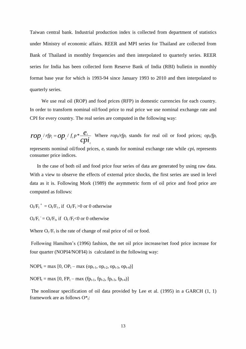
We use real oil (ROP) and food prices (RFP) in domestic currencies for each country.

In order to transform nominal oil/food price to real price we use nominal exchange rate and

CPI for every country. The real series are computed in the following way:

/ / * tt t

t t

t

rfp f p erop opcpi

Where ropt/rfpt stands for real oil or food prices; opt/fpt

represents nominal oil/food prices, et stands for nominal exchange rate while cpit represents

consumer price indices.

In the case of both oil and food price four series of data are generated by using raw data.

With a view to observe the effects of external price shocks, the first series are used in level

data as it is. Following Mork (1989) the asymmetric form of oil price and food price are

computed as follows:

Ot/Ft +

= Ot/Ft , if Ot/Ft >0 or 0 otherwise

Ot/Ft - = Ot/Ft, if Ot /Ft<0 or 0 otherwise

Where Ot /Ft is the rate of change of real price of oil or food.

Following Hamilton’s (1996) fashion, the net oil price increase/net food price increase for

four quarter (NOPI4/NOFI4) is calculated in the following way:

NOPIt = max [0, OPt – max (opt-1, opt-2, opt-3, opt-4)]

NOFIt = max [0, FPt – max (fpt-1, fpt-2, fpt-3, fpt-4)]

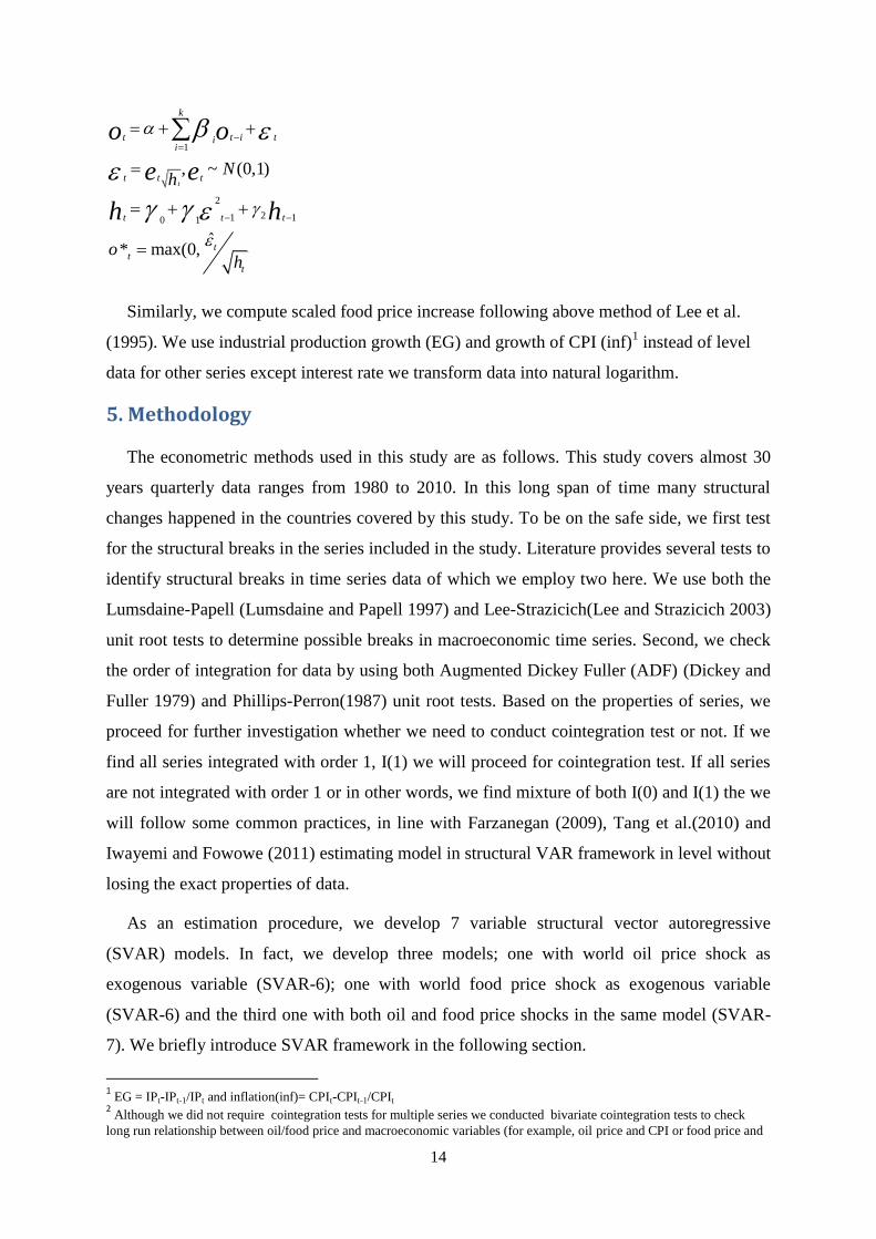
The nonlinear specification of oil data provided by Lee et al. (1995) in a GARCH (1, 1)

framework are as follows O*t:

14

1

2

21 10 1

, ~ (0,1)

ˆ* max(0,

t

k

t t i tii

t t t

t t t

tt

t

Nh

oh

o o

e e

h h

Similarly, we compute scaled food price increase following above method of Lee et al.

(1995). We use industrial production growth (EG) and growth of CPI (inf)1 instead of level

data for other series except interest rate we transform data into natural logarithm.

5. Methodology

The econometric methods used in this study are as follows. This study covers almost 30

years quarterly data ranges from 1980 to 2010. In this long span of time many structural

changes happened in the countries covered by this study. To be on the safe side, we first test

for the structural breaks in the series included in the study. Literature provides several tests to

identify structural breaks in time series data of which we employ two here. We use both the

Lumsdaine-Papell (Lumsdaine and Papell 1997) and Lee-Strazicich(Lee and Strazicich 2003)

unit root tests to determine possible breaks in macroeconomic time series. Second, we check

the order of integration for data by using both Augmented Dickey Fuller (ADF) (Dickey and

Fuller 1979) and Phillips-Perron(1987) unit root tests. Based on the properties of series, we

proceed for further investigation whether we need to conduct cointegration test or not. If we

find all series integrated with order 1, I(1) we will proceed for cointegration test. If all series

are not integrated with order 1 or in other words, we find mixture of both I(0) and I(1) the we

will follow some common practices, in line with Farzanegan (2009), Tang et al.(2010) and

Iwayemi and Fowowe (2011) estimating model in structural VAR framework in level without

losing the exact properties of data.

As an estimation procedure, we develop 7 variable structural vector autoregressive

(SVAR) models. In fact, we develop three models; one with world oil price shock as

exogenous variable (SVAR-6); one with world food price shock as exogenous variable

(SVAR-6) and the third one with both oil and food price shocks in the same model (SVAR-

7). We briefly introduce SVAR framework in the following section.

1 EG = IPt-IPt-1/IPt and inflation(inf)= CPIt-CPIt-1/CPIt

2 Although we did not require cointegration tests for multiple series we conducted bivariate cointegration tests to check

long run relationship between oil/food price and macroeconomic variables (for example, oil price and CPI or food price and

15

5.1 Structural vector autoregressive (SVAR) model specification

We start with the following structural VAR(p) model as provided by Breitung et al.(2004).

1 1 ..........t t p t p t

Where A is a k x k invertible matrix of structural coefficients, Xt is the vector of

endogeneous variables (SPIt, REERt, IRt, INFt, EGt, OPt/FPt), t ~ (0, ). Ais are k x k

matrices which captures dynamic interactions between the k variables while B is another k x k

matrix of structural coefficients representing effects of structural shocks and p is the number

of lagged terms which will be determined by information criteria, SC.

The corresponding estimable reduced form model can be obtained by pre-multiplying the

above model with inverse of matrix A, A-1

as written below:

* *

1 1 ..........t t p t p t

Where Ai* is equal to A

-1Ai. The reduced form residuals relates to the structural residuals

as follows:

1

t t Or, t t

Where ~ (0, andare k x k matrices to be estimated while is the variance

covariance matrix of reduced form residuals and contains k(k+1) distinct elements (Amisano

and Giannini 1997).

In the next step, to identify structural form parameters we have to place restrictions on the

parameter matrices. To make model parsimonious and to avoid invalid restrictions, consistent

with common practices, we place just/exact identifying restrictions. The main assumptions

regarding parameter restrictions are as follows. We assume that structural variance

covariance matrix; is a diagonal matrix and is normalized to be an identity matrix, Ik. We

follow recursive identification scheme and thus we assume that A is an identity matrix while

B is an upper triangular matrix. The contemporaneous relationships among the variables are

captured by B.

Once we have defined our matrices, we now need the number of restrictions. According to

Breitung et al.(2004), when one of the A or B matrix is assumed to be identity then we need

K(K-1)/2 additional restrictions to be placed, where K is the number of variables. In our case

we have 6 variables and 7 variables models; therefore, we need 15 (6 variables) or 21(7

variables) additional restrictions to estimate models.

16

For these additional restrictions we look into the economic theory. Let us first introduce

our 6 variable SVAR model with external oil price. Regardless of the economic conditions of

eight different economies covered by this study we assume, in line with Tang et al.(2010),

that oil price is exogenous and other variables are endogenous. We order variables as (spi,

reer, ir, inf, ip and op) for the 6 variable model with oil price. Oil price is included in the

model in different format of nonlinear transformation as mentioned in the data section. The

matrix format of the ordering is as follows:

=

11 12 13 14 15 16

22 23 24 25 26

33 34 35 36

44 45 46

55 56

66

0

0 0

0 0 0

0 0 0 0

0 0 0 0 0

b b b b b b

b b b b b

b b b b

b b b

b b

b

inf

spi

reer

ir

eg

op

For this ordering, we assume that oil price shock is not affected contemporaneously by

other shocks and it can affect all other endogenous variables and thus we place 5 restrictions

here, (op = b66.op). Second, we assume that industrial production or economic growth is

affected by itself and oil prices and hence we put 4 restrictions (eg = b55.eg+ b56.op). Third,

we assume that for the contemporaneous period inflation/CPI shock is only affected by itself,

output shock and oil price shock while these three affect all other variables. Here we put 3

restrictions, (inf = b44.inf + b45.eg+ b46.op). Fourth shock in the list is short term interest

rate. We assume that it is not affected by real exchange rate and stock price shocks (2

restrictions) for the contemporaneous period while it is affected by all other shocks, (ir =

b33.ir + b34.inf + b35.eg+ b36.op). For the remaining 1 restriction, we assume stock price

shock do not affect real exchange rate while all other shocks may influence it, (reer = b22.reer

+ b23.ir + b24.inf + b25.eg+ b26.op).

Similarly, we construct order for our next model of 6 variables with world food price

shock as exogenous variable. We just replace oil price with food price and hence the order

becomes as (spi, reer, ir, inf, ip and fp). Food price shocks will be used in different formats of

nonlinear transformations. We check the effects of food prices on macroeconomic variables

because recent increase food prices attracted attention for all concerned. In our sample, we

have both food net exporters and net food importer countries; therefore, we can distinguish

17

the magnitudes and signs of effects. Food prices can affect economic growth because it will

increase import bill for the importer countries which reduces net export. For the exporter

countries, when prices increase the demand may decrease which affects export and thus the

output growth. When international food prices increase, it transmits to other countries

through different channels. The arguments we make for oil price model also applies to food

price models and thus we do not repeat those here. The matrix representation of the

restrictions for second model is as follows:

=

11 12 13 14 15 16

22 23 24 25 26

33 34 35 36

44 45 46

55 56

66

0

0 0

0 0 0

0 0 0 0

0 0 0 0 0

b b b b b b

b b b b b

b b b b

b b b

b b

b

inf

spi

reer

ir

eg

fp

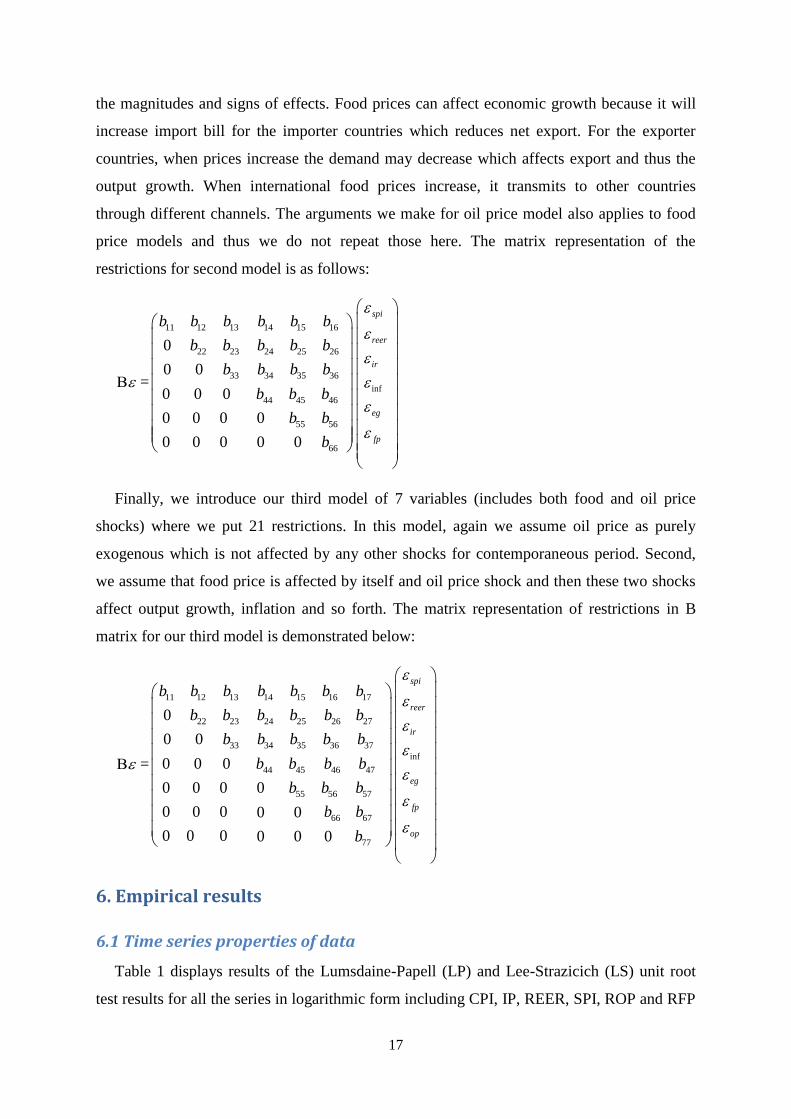
Finally, we introduce our third model of 7 variables (includes both food and oil price

shocks) where we put 21 restrictions. In this model, again we assume oil price as purely

exogenous which is not affected by any other shocks for contemporaneous period. Second,

we assume that food price is affected by itself and oil price shock and then these two shocks

affect output growth, inflation and so forth. The matrix representation of restrictions in B

matrix for our third model is demonstrated below:

=

11 12 13 14 15 16 17

22 23 24 25 26 27

33 34 35 36 37

44 45 46 47

55 56 57

66 67

77

0

0 0

0 0 0

0 0 0 0

0 0 0 0 0

0 0 0 0 0 0

b b b b b b b

b b b b b b

b b b b b

b b b b

b b b

b b

b

inf

spi

reer

ir

eg

fp

op

6. Empirical results

6.1 Time series properties of data

Table 1 displays results of the Lumsdaine-Papell (LP) and Lee-Strazicich (LS) unit root

test results for all the series in logarithmic form including CPI, IP, REER, SPI, ROP and RFP

18

while lending rate LR is at non-log form. The tests are conducted on the original series only

because we assume that breaks (if determined) appear in any series would also be applicable

to transformed series, for example, if any break date is found in CPI it would be the same for

inflation, growth rate CPI. Table1 shows that none of the Australian macroeconomic

variables show any structural break over the period 1980-2010. All series are found to be

nonstationary with the only exception of interest rate series without any break. Consumer

price index series for New Zealand is found to be stationary at 5 percent level of significance

and LS test identified a trend break at the third quarter of 1989. All other series for New

Zealand are nonstationary without any break over 1980-2010 periods. All of the Korean

macroeconomic series are found to be nonstationary identified by both LP and LS tests.

While no breaks are identified in any of the series, in CPI an intercept break has been

detected at fourth quarter of 1997 by LS test. In the case of Singapore, as per the results of LP

test, industrial production index and interest rate series are stationary without break while all

other series are nonstationary without any break. According to LS test, consumer price index

and interest rate series are stationary while LP test results show all series are nonstationary.

Real effective exchange rate is found to be nonstationary with break at the fourth quarter of

2001 by LS test. While LP test results show all the Taiwanese series are nonstationary

without any break, LS test results reveal that IP and SPI are stationary with break at first

quarter of 2009 and second quarter of 2008 respectively. ROP and RFP are found to be

stationary without any break. In addition, LS test also identified that REER is nonstationary

with a break at the second quarter of 2008. The Indian macroeconomic series are found to be

nonstationary without any break by LP test except real effective exchange rate. Real effective

exchange rate is found to be stationary with two breaks at third quarter of 1998 and fourth

quarter of 2004. LP test results show that IP, REER and LR series are stationary without any

break while all other series are nonstationary. Thai real effective exchange rate is found

stationary with break at the first quarter of 1997 by LP test while all other series are

nonsationary. LS test results indicate that CPI and RFP are stationary while all other series

are nostationary without any break.

As discussed above, macroeconomic series of Australia and Singapore have no structural

breaks while few series of other countries show structural breaks. Excepting Taiwan, in the

case of the rest of the countries one series is found to have structural break. Since both LP

and LS tests do not indicate breaks commonly and except one series other series are free of

break we estimate models with full sample of data for these countries. As three series of

19

Taiwan are found with break during the second quarter of 2008 we intended to estimate

model for Taiwan for the sample until the first quarter of 2008. However, because of the

unavailability enough observations we cannot split samples into two and thus we estimate full

sample in the case of Taiwan as well.

According to Table 1, IR series for Australia; CPI and ROP for New Zealand; IP and IR

for Singapore; CPI and IR for Hong Kong; IP, SPI, ROP and RFP for Taiwan; IP, REER and

IR for India; and REER and RFP for Thailand are stationary at level.

Table 1 Unit root test using structural break

Country Lumsdaine-Papell Unit Root Test Lee-Strazicich Unit Root Test

Series

TB1

TB2

Y t-1 D1t DT1t D2t DT2t TB1

TB2

S t-1 D1t DT1t D2t DT2t

AUS

CPI 1989:1

2000:2

-0.198

(-5.899)

0.012

(3.498)

-0.002

(-5.681)

0.006

(2.529)

0.000

(3.329)

1988:4

1998:1

-0.212

(-5.189)

-0.005

(-0.882)

-0.007

(-4.486)

0.003

(0.577)

-0.007

(-3.908)

IP 1984:4

1999:2

-0.262

(-4.975)

0.025

(2.757)

0.001

(1.326)

0.027

(3.469)

-0.001

(-4.211)

1988:1

1999:2

-0.424

(-4.422)

-0.031

(-1.823)

0.017

(2.718)

0.003

(0.178)

0.018

(2.961)

REER 1984:4

2002:4

-0.292

(-5.240)

-0.063

(-3.017)

-0.001

(-0.063)

0.038

(2.129)

0.002

(2.504)

1985:2

1999:3

-0.413

(-4.842)

0.066

(1.555)

-0.047

(-2.626)

-0.002

(-0.064)

-0.009

(-1.080)

IR 1988:4

1994:1

-0.330a

(-7.292)

1.311

(3.128)

-0.208

(-5.466)

0.354

(1.162)

0.177

(5.394)

1988:3

1992:3

-0.563

(-6.493)

0.449

(0.708)

-0.624

(-3.145)

0.840

(1.400)

-1.107

(-3.972)

SPI 1984:4

2005:2

-0.263

(-4.930)

0.131

(2.876)

0.000

(0.250)

0.107

(2.465)

-0.007

(-2.718)

1985:3

2003:4

-0.441

(-4.870)

-0.096

(-1.170)

0.103

(2.722)

-0.061

(0.771)

0.012

(0.727)

ROP 1985:4

1999:3

-0.469

(6.368)

-0.347

(-4.559)

0.000

(0.147)

0.222

(3.859)

0.009

(3.398)

1987:1

1999:2

-0.517

(-5.333)

-0.024

(-0.170)

-0.101

(-2.192)

0.069

(0.471)

0.185

(0.434)

RFP 1988:3

2002:4

-0.464

(-6.402)

-0.115

(-3.815)

0.002

(1.670)

-0.092

(-3.137)

0.002

(2.163)

1988:2

2008:1

-0.411

(-5.314)

0.084

(1.315)

-0.067

(-3.371)

0.030

(0.465)

0.047

(2.001)

NZ

CPI 1986:3

1998:3

-0.181b

(-6.847)

0.033

(5.251)

-0.003

(-6.458)

-0.009

(-2.622)

0.000

(1.215)

1989:03

1999:03

-0.403

(-5.508)

0.011

(1.362)

-0.035a

(-11.180)

-0.001

(-0.149)

-0.005

(-2.455)

MP 1994:4

2002:1

-0.204

(-4.464)

0.078

(4.642)

-0.000

(-1.322)

0.046

(3.426)

-0.000

(-0.593)

1986:2

1994:3

-0.240

(-4.181)

0.071

(2.463)

-0.032

(-3.026)

-0.037

(-1.294)

0.064

(4.098)

REER 1986:3

2003:3

-0.197

(-4.684)

0.050

(2.983)

0.000

0.540

0.051

(3.113)

0.000

(0.279)

1985:4

2000:1

-0.243

(-4.738)

-0.0145

(-0.404)

0.030

(2.558)

0.005

(0.166)

-0.010

(-1.325)

IR 1992:1

1998:2

-0.288

(-6.401)

-0.958

(-3.233)

0.110

(3.495)

-1.120

(-4.619)

-0.010

(-0.771)

1993:1

1999:2

-0.288

(-6.401)

-0.958

(-3.233)

0.110

(3.495)

-1.120

(-4.619)

-0.010

(-0.771)

SPI 1987:3

2005:2

-0.275

(-5.309)

-0.262

(-5.138)

-0.012

(-3.765)

0.084

(1.492)

-0.011

(-2.969)

1987:2

1993:1

-0.285

(-4.439)

0.287

(2.580)

-0.161

(-4.493)

-0.056

(-0.521)

0.207

(4.613)

ROP 1985:4

1999:1

-0.442c

(-6.549)

-0.424

(-5.093)

0.000

(0.129)

0.231

(3.988)

0.010

(3.446)

1985:3

1999:3

-0.432

(-5.093)

0.420

(2.668)

-0.275

(-4.079)

0.034

(0.220)

0.317

(5.042)

RFP 1986:3

2002:3

-0.338

(-5.561)

-0.0138

(-0.378)

0.001

(0.911)

-0.092

(-3.021)

0.004

(3.135)

1986:3

2007:4

-0.393

(-4.579)

-0.125

(0.160)

-0.056

(-2.649)

0.115

(1.682)

0.053

(2.157)

KOR

CPI 1989:4

1998:2

-0.239

(-5.848)

0.022

(4.511)

0.000

(3.543)

-0.006

(-1.032)

-0.001

(5.878)

1991:3

1997:4

-0.0842

(-5.244)

0.003

(0.539)

-0.005

(-2.919)

0.041a

(7.064)

-0.006

(-4.556)

IP 187:1

1999:2

-0.506

(-5.267)

0.070

(2.925)

-0.006

(-4.248)

0.062

(3.541)

-0.000

(-1.559)

1988:2

1999:3

-0.849

(-5.694)

0.107

(3.429)

0.010

(1.211)

0.061

(1.930)

-0.023

(-3.060)

REER 1997:3

2005:4

-0.362

(-6.636)

-0.187

(-6.045)

-0.001

(-1.156)

0.090

(2.590)

-0.012

(-4.711)

1997:2

2004:2

-0.326

(-5.041)

0.087

(1.590)

-0.067

(-4.310)

-0.008

(-0.162)

0.103

(4.311)

IR 1993:4

1998:2

-0.174

(-5.880)

-0.710

(-2.092)

0.128

(4.255)

-1.766

(-5.234)

-0.125

(-4.147)

1985:2

1999:1

-0.170

(-4.073)

-0.181

(-0.305)

0.522

(2.327)

-0.518

(-0.851)

-0.212

(-1.740)

SPI 1986:4

1997:3

-0.251

(-5.596)

0.300

(4.203)

-0.006

(-2.034)

-0.161

(-2.995)

0.005

(3.504)

1987:3

1997:3

-0.3281

(-5.055)

-0.210

(-1.890)

0.178

(3.327)

-0.374

(-3.605)

-0.063

(-2.343)

ROP 1985:4

1993:2

-0.557

(-6.296)

-0.388

(-4.289)

0.002

(0.398)

-0.225

(-3.270)

0.018

(3.732)

1987:4

1997:1

-0.514

(-6.019)

-0.115

(-0.723)

-0.077

(-1.706)

-0.146

(-0.919)

0.114

(3.129)

RFP 1988:3

2004:2

-0.372

(-5.103)

-0.114

(-2.988)

0.003

(1.951)

-0.106

(-2.650)

0.010

(3.915)

1995:2

2006:1

-0.457

(-4.927)

0.017

(0.216)

0.050

(2.749)

0.035

(0.436)

-0.005

(-0.216)

SIN

CPI 1990:3

2004:3

-0.116

(-4.752)

0.009

(3.588)

-0.000

(-0.176)

-0.005

(-1.598)

0.001

(3.476)

1990:4

2001:1

-0.097

(-4.163)

-0.001

(-0.153)

-0.002

(-1.902)

0.000

(0.063)

-0.003

(-2.615)

IP 1987:1

2000:4

-0.529b

(-7.112)

0.134

(4.300)

0.008

(4.246)

-0.080

(4.246)

-0.001

(-0.446)

1985:4

1991:2

-0.764

(-4.998)

-0.134

(-2.264)

0.050

(2.342)

0.030

(0.506)

-0.098

(-4.632)

REER 1985:4

1998:2

-0.161

(-3.550)

-0.044

(-4.192)

-0.001

(-2.790)

-0.033

(-5.256)

-0.001

(-3.858)

1993:2

2001:3

-0.134

(-4.518)

0.000

(0.004)

0.011

(2.959)

-0.027

(-1.985)

-0.012

(-2.681)

IR 1986:2 -0.444a -0.849 0.128 -0.418 -0.036 1886:1 -0.314 0.125 -0.290 -0.156 0.104

20

1991:4 (-7.734) (-3.695) (5.289) (-2.637) (-3.012) 1998:4 (-3.922) (0.447) (-1.867) (-0.514) (1.862)

SPI 1993:2

2004:2

-0.356

(-5.149)

0.097

(1.726)

-0.010

(-3.189)

0.133

(2.158)

0.004

(1.226)

1993:1

2001:4

-0.728

(-5.123)

-0.015

(-0.148)

0.089

(2.596)

0.232

(2.204)

-0.118

(-3.549)

ROP 1985:4

1999:1

-0.419

(-5.428)

-0.206

(-2.942)

0.004

(0.786)

0.214

(3.785)

0.015

(3.892)

1990:1

1998:4

-0.770

(-5.117)

-0.326

(-2.256)

0.177

(3.878)

-0.285

(-1.910)

0.278

(4.944)

RFP 1991:1

1998:2

-0.377

(-5.110)

-0.106

(-3.906)

0.002

(2.022)

-0.060

(-2.653)

0.004

(2.170)

1991:1

2003:1

-0.336

(-4.755)

-0.049

(-0.954)

-0.023

(-1.745)

-0.023

(-0.448)

0.057

(3.759)

HK

CPI 1994:1

2006:1

-0.059

(-3.943)

0.011

(2.232)

-0.001

(-4.271)

0.003

(0.759)

0.001

(1.815)

1994:1

2002:4

-0.147a

(-5.931)

0.009

(1.245)

-0.003

(-0.919)

0.007

(0.889)

-0.015

(-4.630)

IP 1986:1

2004:4

-0.309

(-6.259)

0.181

(5.492)

0.003

(0.704)

0.262

(8.987)

-0.008

(-4.746)

1990:1

2001:1

-0.475

(-5.807)

0.048

(1.297)

-0.045

(-4.256)

0.06

(2.184)

-0.084

(-4.922)

REER 1986:4

1996:4

-0.171

(-5.230)

-0.169

(-1.004)

0.011

(3.768)

0.052

(3.429)

-0.004

(-5.582)

1992:2

2001:4

-0.193

(-3.841)

-0.063

(-2.564)

0.040

(4.219)

0.052

(2.153)

-0.061b

(-5.861)

IR 1991:2

2000:4

-0.207

(-5.258)

-1.850

(-4.367)

0.020

(3.291)

-0.958

(-4.463)

-0.018

(-2.115)

1997:2

2004:4

-0.501c

(-5.542)

-0.516

(-1.445)

0.695

(3.510)

-0.537

(-1.478)

0.390

(3.820)

SPI 1999:1

2003:3

-0.342

(-4.248)

0.184

(2.482)

-0.015

(-2.032)

0.124

(1.936)

0.020

(3.088)

2000:1

2005:2

-0.876

(-4.947)

0.032

(0.267)

-0.043

(-1.121)

-0.112

(-0.966)

0.256

(4.543)

ROP 1985:4

1999:1

-0.408

(-5.320)

-0.220

(-2.935)

-0.002

(-0.454)

0.164

(2.997)

0.021

(4.359)

1997:2

2005:3

-0.433

(-5.230)

0.068

(0.474)

0.018

(0.557)

-0.159

(-1.107)

0.121

(2.534)

RFP 1989:1

1998:2

-0.347

(-5.133)

-0.058

(-2.351)

-0.004

(-2.418)

-0.080

(-2.909)

0.012

(4.818)

1990:4

2000:1

-0.358

(-5.281)

0.013

(0.287)

-0.035

(-2.656)

0.008

(01.167)

0.044

(4.091)

TWN

CPI 1986:4

1994:1

-0.281

(-5.084)

-0.008

(-1.502)

0.003

(5.038)

0.009

(1.902)

-0.002

(-5.552)

1993:2

2000:3

-0.269

(-5.131)

-0.028

(-3.261)

0.013

(3.434)

0.023

(2.829)

-0.010

(-4.019)

IP 1988:1

2006:2

-0.189

(-3.380)

0.633

(3.469)

0.003

(2.608)

0.004

(1.247)

-0.002

(-2.164)

2006:4

2009:1

-0.418a

(-19.68)

0.006

(2.267)

-0.008

(-4.730)

0.018

(5.841)

-0.027

(-13.45)

REER 1988:2

2003:4

-0.521

(-4.664)

2.647

(4.619)

-0.004

(-3.070)

0.030

(2.947)

0.002

(1.638)

2004:1

2008:2

-2.138

(-6.349)

0.018

(1.312)

0.008

(1.136)

0.068

(3.863)

-0.075a

(-6.361)

IR 1989:1

2002:4

-0.227

(-5.416)

1.043

(4.287)

0.039

(3.270)

-0.765

(-3.641)

0.013

(1.630)

1988:4

2004:2

-0.312

(-5.170)

-0.969

(-2.239)

1.374

(5.054)

-0.115

(-0.291)

-0.573

(-3.857)

SPI 2001:1

2006:2

-0.576

(-4.599)

-0.231

(-2.127)

0.036

(1.436)

0.076

(1.031)

-0.012

(-1.745)

2002:4

2008:2

-4.294a

(-7.067)

-0.142

(-1.717)

0.013

(0.216)

0.029

(0.413)

-0.387

(-7.601a)

ROP 1985:4

1997:4

-0.468

(-5.919)

-0.247

(-3.245)

0.003

(0.469)

-0.194

(-3.205)

0.015

(4.695)

1989:3

1999:1

-0.413c

(-5.619)

0.018

(0.124)

0.124

(2.810)

0.234

(1.610)

0.003

(0.080)

RFP 1995:2

2001:1

-0.380

(-4.781)

0.065

(2.030)

-0.010

(-3.936)

-0.042

(-1.320)

0.017

(4.827)

1995:4

2000:4

-0.430c

(-5.432)

0.043

(0.750)

0.016

(0.915)

0.230

(3.965)

-0.041

(-1.823)

IN

CPI 1997:4

2006:2

-0.263

(-4.421)

0.019

(2.513)

-0.003

(-4.711)

-0.006

(-0.664)

0.004

(4.702)

1994:2

2003:4

-0.203

(-4.334)

-0.002

(-0.161)

0.001

(0.408)

0.010

(0.827)

-0.013

(-2.442)

IP 1991:1

2000:4

-0.448

(-4.275)

-0.075

(-5.204)

-0.001

(-0.685)

-0.064

(-4.278)

0.001

(1.357)

1989:1

2000:2

-0.633c

(-5.408)

-0.087

(-3.090)

0.060

(4.647)

0.029

(1.077)

-0.028

(-3.608)

REER 1998:3

2004:4

-0.828a

(-14.45)

-0.448a

(-13.81)

0.007

(5.045)

0.266

(10.09)

-0.011a

(-8.11)

1998:3

2005:1

-0.714c

(-5.683)

0.215

(2.869)

-0.236

(-5.016)

-0.010

(-0.155)

0.222

(5.070)

IR 1991:1

1996:2

-0.205

(-4.124)

-0.048

(-2.205)

-0.048

(-2.215)

-0.246

(-0.969)

0.039

(1.909)

1996:2

2006:3

-0.474c

(-5.643)

-0.373

(-0.683)

-0.901

(-5.150)

-0.857

(-1.577)

1.2243

(4.166)

SPI 1991:1

2004:3

-0.276

(-6.169)

0.2857

(4.800)

-0.010

(-4.654)

0.174

(3.162)

0.007

(2.289)

1991:3

2001:3

-0.318

(-4.853)

-0.069

(-0.582)

0.135

(2.961)

-0.056

(-0.489)

-0.047

(-1.509)

ROP 1985:4

1997:4

-0.501

(-6.402)

-0.033

(-4.091)

0.011

(2.094)

-0.152

(-2.671)

0.010

(3.593)

1990:1

1998:2

-0.401

(-5.164)

-0.340

(-2.384)

0.241

(4.385)

-0.292

(-2.031)

0.016

(0.520)

RFP 1988:1

1998:2

-0.394

(-5.724)

0.072

(2.681)

0.005

(2.995)

-0.133

(-4.231)

0.000

(0.230)

1987:2

1998:2

-0.368

(-4.789)

-0.070

(-1.253)

0.063

(3.253)

-0.127

(-2.270)

-0.052

(-3.412)

TH

CPI 1989:1

1996:1

-0.179

(-4.671)

0.006

(1.534)

0.001

(4.175)

-0.012

(-3.093)

-0.001

(-3.568)

1990:2

1999:1

-0.218c

(-5.331)

-0.018

(-0.974)

-0.007

(-2.262)

-0.012

(-1.507)

-0.009

(-4.878)

IP 1997:1

2003:2

-0.376

(-5.481)

-0.072

(-3.893)

-0.001

(-0.121)

0.048

(2.926)

-0.001

(-1.441)

1998:1

2008:1

-0.652

(-4.983)

-0.014

(-0.494)

-0.048

(-2.682)

0.037

(1.273)

-0.056

(-0.056)

REER 1997:1

2005:2

-0.739a

(-8.445)

-0.172a

(-8.521)

-0.009

(3.902)

0.059

(3.902)

0.006

(4.089)

1998:1

2003:3

-0.619

(-6.008)

-0.098

(-2.227)

-0.017

(-0.841)

-0.007

(-0.191)

0.009

(0.937)

IR 1985:4

1998:3

-0.196

(-5.902)

-0.823

(-3.019)

0.016

(0.894)

-1.408

(-5.460)

-0.011

(-1.496)

1994:2

2001:4

-0.340

(-5.281)

0.885

(1.675)

0.412

(2.848)

0.171

(0.340)

-0.674

(-3.468)

SPI 1998:1

2003:3

-0.501

(-4.861)

-0.159

(-1.420)

0.198

(1.300)

0.286

(3.115)

0.001

(0.142)

2001:3

2008:1

-0.434

(-4.424)

-0.253

(-2.485)

0.230

(4.265)

0.194

(1.789)

-0.242

(-3.846)

ROP 1985:4

1999:1

-0.457

(-5.912)

-0.270

(-3.584)

0.003

(0.648)

0.249

(4.104)

0.012

(3.635)

1995:2

2008:1

-0.487

(-5.293)

-0.129

(-0.879)

0.111

(3.536)

0.442

(2.878)

-0.170

(-3.192)

RFP 1997:2

2002:2

-0.435

(-6.010)

0.127

(3.504)

-0.001

(-0.643)

0.069

(2.039)

0.006

(2.224)

1987:3

1991:4

-0.654b

(-5.783)

-0.071

(-1.122)

0.074

(2.802)

0.065

(1.047)

-0.053

(-2.537)

Next, we employ conventional unit root tests to determine the order of integration for the

nonstationary series along with some transformed series of IP, CPI, OP and FP for all

countries. Table 2 presents results of unit root tests conducted by augmented Dickey-Fuller

21

(ADF) and Phillips-Perron(PP) unit root test. Unit root tests reveal that the evidence of

stationarity for level series is mixed while all transformed series are stationary at level. It can

be noted that for Australia all series are nonstationary at level while they are stationary at first

difference. IR and REER series for New Zealand and Korea are found to be stationary at

level while all other series are stationary at first difference. Almost all the series for all other

countries are found stationary at their first differences.

Having established the order of integration we proceed for the VAR estimation procedure

particularly SVAR. As discussed in the methodology section, we do not go for cointegration

because we have found the mixed evidence of I (0) and I (1) order among the series2.

Table 2 Results of unit root tests AUS NZ KOR SIN HK TWN IN TH

CPI I(1) I(0) I(1)* I(1) I(0) I(1) I(1) I(1)

INF I(0) I(0) I(0) I(0) I(0) I(0) I(0) I(0)

SPI I(1) I(1) I(1) I(1) I(1) I(0) I(1) I(1) IR I(0) I(0) I(0) I(0) I(0) I(1) I(0) I(1)

REER I(1) I(0)* I(0)* I(1) I(1) I(1) I(0) I(0)

IP I(1) I(1) I(1) I(0) I(1)* I(0) I(0) I(1) EG I(0) I(0) I(0) I(0) I(0) I(0) I(0) I(0)

RFP I(1) I(1) I(1) I(1) I(1) I(0) I(1) I(0)

NOFI I(0) I(0) I(0) I(0) I(0) I(0) I(0) I(0) FP+ I(0) I(0) I(0) I(0) I(0) I(0) I(0) I(0)

FP- I(0) I(0) I(0) I(0) I(0) I(0) I(0) I(0)

SOFI I(0) I(0) I(0) I(0) I(0) I(0) I(0) I(0) LROP I(1) I(0) I(1) I(1) I(1) I(0) I(1) I(1)

OP+ I(0) I(0) I(0) I(0) I(0) I(0) I(0) I(0)

OP- I(0) I(0) I(0) I(0) I(0) I(0) I(0) I(0) NOPI I(0) I(0) I(0) I(0) I(0) I(0) I(0) I(0)

SOPI I(0) I(0) I(0) I(0) I(0) I(0) I(0) I(0)

Note: Unit root tests have been performed by both ADF (Augmented Dickey-Fuller) and PP (Phillips-Perron) methods. I(1) implies that the series is nonsationary at level,

however, stationary at first differences which is confirmed by both ADF and PP test.

Bold I(0) indicates series are stationary at level either in LP or LS test I(0) indicates that series is stationary at level.

I(0)* represents that the series is level stationary at ADF test while it is nonstationary at PP test

I(1)* means the series is level nonstationary at ADF while in PP it is stationary

Now we turn to estimate the VAR models. We estimate models with different

specifications of oil and food prices. For the brevity purpose we do not report all results. We

identify the relative performance of models based on the lowest information criteria. Both

AIC and SC criteria as shown in Table 3 indicate that models with NOPI as proxy for oil

price and NOFI as proxy for food prices perform better than models that include other

specifications. Therefore we report results of SVAR models only with NOPI and NOFI

specifications.

2 Although we did not require cointegration tests for multiple series we conducted bivariate cointegration tests to check

long run relationship between oil/food price and macroeconomic variables (for example, oil price and CPI or food price and

IP). Tests results provide no evidence of cointegration between oil/food price and any macroeconomis series.

22

Table 3 Relative performance of models Models with CPI and IP at levels Models with CPI and IP in growth rate

Country Models AIC SC AIC SC

Australia

ROP (RFP)

-17.07697 (-18.69567)

-16.10653 (-17.72523)

1.643486 (0.109013)

2.619108 (1.084635)

NOPI4

(NOFI4)

-19.01105

(-20.54233)

-18.02487

(-19.55616)

-0.286658

(-1.800708)

0.699518

(-814532)

ROP+ (RFP+)

-9.170613 (-18.45812)

-8.194991 (-1748249)

9.526793 (0.250267)

10.50241 (1.225889)

ROP-

(RFP-)

-7.978330

(-18.00280)

-7.002708

(-17.02718)

10.75997

(0.720651)

11.73559

(1.696273)

SOPI (SOFI)

-18.25596 (-13.09202)

-1727509 (-12.11115)

0.479859 (5.664741)

1.460726 (6.545608)

New Zealand

ROP

(RFP)

-17.31332

(-19.07781)

-16.17695

(-17.94145)

1.584934

(-0.371090)

2.721300

(0.765276)

NOPI4 (NOFI4)

-18.96624 (-20.72100)

-1782987 (-19.58463)

-0.255700 (-2.027159)

0.880665 (-0.890793)

ROP+

(RFP+)

-8.903014

(-9.714522)

-7.766648

(-8.5781157)

9.879078

(9.020350)

11.01544

(10.15672)

ROP- (RFP-)

-7.818844 (-9.078588)

-6.682479 (-7.942222)

10.92942 (9.575373)

12.06579 (10.71174)

SOPI

(SOFI)

-13.54162

(-13.16695)

-12.40525

(-12.03059)

5.208307

(5.530642)

6.344672

(6.667008)

Korea

ROP (RFP)

-13.35477 (-14.87795)

-12.30562 (-13.82880)

4.978935 (3.621604)

6.028082 (4.670752)

NOPI4

(NOFI4)

-15.30315

(-16.81988)

-14.25400

(-15.77073)

3.022300

(1.604145)

4.071447

(2.653292)

ROP+ (RFP+)

7.967950 (7.149424)

9.017098 (8.198572)

26.32318 (25.66092)

27.37232 (26.71007)

ROP-

(RFP-)

9.108107

(7.671566)

10.15725

(8.720713)

27.40921

(26.00336)

28.45836

(27.05251)

SOPI (SOFI)

-9.931060 (-1067466)

-8.881912 -9.619333

8.424427 (7.734274)

9.473575 (8.789599)

Singapore

ROP

(RFP)

-18.54292

(-20.63708)

-17.46856

(-19.56273)

-0.076817

(-2.089581)

0.997538

(-1.015225)

NOPI4 (NOFI4)

-20.39027 (-22.57345)

-19.31591 (-21.49909)

-1.913455 (-4.138210)

-0.8390099 (-3.063854)

ROP+

(RFP+)

-10.34260

(-11.40764)

-9.268242

(-10.33329)

8.195938

(7.013105)

9.270290

(8.087461)

ROP- (RFP-)

-9.041827 (-10.78621)

-8.041827 (-9.711856)

9.474217 (7.728441)

10.54857 (8.802796)

SOPI

(SOFI)

-14.76252

(-14.66159)

-13.68816

(-13.58072)

3.701210

(3.808571)

4.775565

(4.889442)

Hong Kong

ROP (RFP)

-15.30287 (-16.92225)

-13.90945 (-15.52884)

-14.73660 (-16.51576)

-13.34318 (-15.12234)

NOPI4

(NOFI4)

-16.33509

(-17.90041)

-1494167

(-16.50699)

-15.84642

(-17.51254)

-14.45300

(-16.11913)

ROP+ (RFP+)

-2.782997 (-4.126986)

-1.389581 (-2.733569)

-2.340396 (-3.824068)

-0.946979 (-2.430652)

ROP-

(RFP-)

-1.522621

(-3.407123)

-0.129205

(-2.013706)

-1.293543

(-3.142687)

0.099874

(-3.142687)

SOPI

(SOFI)

-11.15229

(-10.51796)

-9.758877

(-9.124541)

-10.79750

(-10.26125)

-9.404079

(-8.867831)

Taiwan

ROP

(RFP)

-27.79412

(-28.06732)

-24.05059

(-24.32379)

-9.806751

(-9.778903)

-6.032461

(-6.004613)

NOPI4

(NOFI4)

-29.41465

(-28.28715)

-25.67112

(-24.54362)

-11.25056

(-10.64074)

-7.476266

(-6.866451)

ROP+

(RFP+)

-11.97108

(-11.49312)

-8.227554

(-7.749592)

6.396268

(6.198128)

10.17056

(9.972418)

ROP-

(RFP-)

-10.92641

(-11.23243)

-7.182885

(-7.488903)

6.964473

(6.708723)

10.73876

(10.48301)

SOPI

(SOFI)

-23.55958

(-21.76764)

-19.81605

(-17.99335)

-5.497711

(-3.939545)

-1.723421

(-0.136653)

India

ROP (RFP)

-12.77136 (-14.43708)

-11.42227 (-13.08799)

6.109153 (4.464949)

7.458250 (5.824046)

NOPI4

(NOFI4)

-14.13250

(-15.82010)

-12.78340

(-14.47100)

4.624968

(3.039586)

5.974065

(4.388683)

ROP+

(RFP+)

2.730818

(1.561440)

4.079915

(1.913111)

21.52521

(20.47275)

22.47430

(21.82185)

ROP-

(RFP-)

4.174667

(2.260601)

5.523764

(3.609699)

22.94593

(21.02763)

24.29523

(22.37673)

SOPI

(SOFI)

-8.574705

(-8.892300)

-7.225608

(-7.543202)

10.21289

(10.13972)

11.56199

(11.48882)

23

Thailand

ROP

(RFP)

-16.97891

(-18.51970)

-15.43193

(-16.97271)

-16.19290

(-17.30175)

-14.64591

(-15.75477)

NOPI4 (NOFI4)

-17.97615 (-19.32396)

-16.42916 (-17.77698)

-16.91605 (-18.38293)

-15.36607 (-16.83594)

ROP+

(RFP+)

-1.619526

(-2.160991)

-0.072539

(-0.614003)

-0.549011

(-1.237080)

-0.997976

0.309907

ROP- (RFP-)

-0.465334 (-1.984002)

-1.081654 (-0.437015)

-0.088004 (-1.274428)

1.458983 (0.272559)

SOPI

(SOFI)

-13.04117

(-12.68016)

-11.49419

(-11.13317)

-12.12896

(-11.82287)

-10.58197

(-10.27588)

Note: Figures are values of information criteria with different specification of oil prices

and values in parentheses are for food price specifications

6.2 Granger causality tests

Table 4 reports results for Granger causality tests for each of the variables. As can be seen,

Australian and New Zealand’s selected macroeconomic variables show similar response to

oil and food price shocks. Only real effective exchange rates are found to be Granger caused

by net oil and food price increase while no evidence of Granger causality can be observed for

other variables. In the case of Korea, excepting stock price indices, Granger causality can be

found for all other variables from both oil and food price increase. Singapore is the only

country where tests fail to show any evidence of Granger causality from oil and food price

increase to any of the variables. Low evidence of causality can be viewed for Hong Kong and

Thailand as well. Unidirectional causality is found form oil price to interest rate and from

food price to real effective exchange rate in Hong Kong. A unidirectional causality from oil

price to industrial production growth is found statistically significant for Thailand while no

evidence can be found for all other variables. In Taiwan, unidirectional causalities from oil

price to all other variables are found to be statistically significant at least at 5 percent level of

significance. However, evidence from food price is statistically significant only for real

effective exchange rate. Marginal evidence of causality form oil and food price shocks are

also evident for some of the India’s macroeconomic variables. Unidirectional causality from

oil price to interest rate and from food price to stock price indices, real effective exchange

rate and industrial growth are statistically significant at 10 percent level of significance.

Table 4 Results of Granger causality/block exogeneity Wald tests Variables AUS NZ KOR SIN HK TWN IN TH

NOPI NOFI NOPI NOFI NOPI NOFI NOPI NOFI NOPI NOFI NOPI NOFI NOPI NOFI NOPI NOFI

SPI 0.49 (0.48)

1.11 (0.29)

2.27 (0.13)

0.06 (0.79)

1.70 (0.19)

0.05 (0.81)

0.05 (0.81)

0.05 (0.82)

0.04 (0.82)

0.52 (0.46)

5.36b

(0.06) 1.59 (0.44)

0.63 (0.42)

3.19c

(0.07) 1.20 (0.27)

0.59 (0.44)

REER 9.28a

(0.00)

3.09c

(0.07)

5.02b

(0.02)

18.82a

(0.00)

33.42a

(0.00)

89.59a

(0.00)

1.82

(0.17)

0.04

(0.83)

0.00

(0.96)

5.19b

(0.02)

23.68a

(0.00)

12.75a

(0.00)

0.43

(0.50)

3.02c

(0.08)

2.14

(0.14)

0.12

(0.72)

IR 0.30

(0.58)

0.02

(0.88)

0.04

(0.83)

0.00

(0.96)

25.23a

(0.00)

80.35a

(0.00)

0.07

(0.77)

0.83

(0.36)

4.92b

(0.02)

0.58

(0.44)

5.27b

(0.07)

2.40

(0.30)

3.63c

(0.05)

1.90

(0.16)

0.34

(0.55)

0.20

(0.65)

INF 0.11 (0.73)

0.09 (0.76)

1.91 (0.16)

0.83 (0.35)

9.36a

(0.00) 21.90a

(0.00) 0.19 (0.65)

0.09 (0.76)

0.86 (0.35)

0.04 (0.83)

6.36b

(0.04) 0.26 (0.87)

0.02 (0.86)

0.00 (0.99)

0.10 (0.74)

1.79 (0.18)

EG 0.00

(0.98)

0.07

(0.78)

0.79

(0.37)

0.68

(0.40)

3.87b

(0.04)

11.57a

(0.00)

0.05

(0.81)

0.74

(0.38)

0.18

(0.66)

0.46

(0.49)

5.05b

(0.07)

3.16

(0.20)

0.01

(0.90)

3.01c

(0.08)

6.11b

(0.01)

0.00

(0.94)

Note: entries are chi-square test statistics at degrees of freedom of 1 in all cases except Taiwan. Degree of

freedom for Taiwan is 2. Lag length are selected by SC criteria. Values in parentheses are p-values.

a, b, c indicate significance at 1%, 5% and 10% level.

24

6.3 Impulse response analysis

Figure 2 displays responses of Australia’s macroeconomic variables to oil and food price

shocks3. Although most of the impulse response functions shown in Figure 3 are not

statistically significant the signs of the responses in most cases are consistent to the theory.

As can be viewed, the stock price indices and the real effective exchange rate respond

negatively with one standard deviation (S.D.) innovation in net oil and food price increase

while interest rate and inflation respond positively. The growth of industrial production

responds negatively with food prices while the response with oil price is positive. Following

the oil price shock, stock price decreases and it takes around 7 quarters to ease off. Real

exchange rates react highly to both oil and food price shocks and do not reach to zero level

even after 15 periods. Interest rate increases by 9 percent following the food price shock

while it increases by approximately 13 percent for oil price shock and reaches to zero level

after around 2 and 7 quarters respectively. Effects of shocks to inflation and industrial growth

are rather short- lived. Positive response of inflation dies out in 3 quarters while it takes only

2 quarters for industrial growth rate (negative to food and positive to oil price shocks).

Figure 2 Impulse responses of Australia macroeconomic variables to NOFI and NOPI

3 We estimated 3 models for every country as stated in the methodology section but we report results for only third model which includes

both oil and food prices because all models produce qualitatively similar results. However, results of other two models are available from authors upon request.

-.100

-.075

-.050

-.025

.000

.025

.050

.075

.100

1 2 3 4 5 6 7 8 9 10 11 12 13 14 15

Response of SPI to NOFI

-.100

-.075

-.050

-.025

.000

.025

.050

.075

.100

1 2 3 4 5 6 7 8 9 10 11 12 13 14 15

Response of SPI to NOPI

-.04

-.02

.00

.02

.04

.06

1 2 3 4 5 6 7 8 9 10 11 12 13 14 15

Response of REER to NOFI

-.04

-.02

.00

.02

.04

.06

1 2 3 4 5 6 7 8 9 10 11 12 13 14 15

Response of REER to NOPI

-0.4

-0.2

0.0

0.2

0.4

0.6

0.8

1.0

1 2 3 4 5 6 7 8 9 10 11 12 13 14 15

Response of IR to NOFI

-0.4

-0.2

0.0

0.2

0.4

0.6

0.8

1.0

1 2 3 4 5 6 7 8 9 10 11 12 13 14 15

Response of IR to NOPI

25

The responses of economic variables of New Zealand to the oil and food price shocks are

presented in Figure 3. All the variables respond, consistent with underlying theories, to oil

and food price shocks. Stock prices, real effective exchange rates and industrial growth

decrease with one S.D. shock from oil or food price while interest rate and inflation respond

positively. Due to the shock in food prices stock prices decrease about 2 percent at the first

quarter and after a slight improvement in the second quarter it remains negative until after 4

years. Although stock prices due to one standard deviation oil price shock do not decrease at

the first quarter it keeps falling until fifth quarter up to 5 percent and then keeps negative

even after 4 years period. Real effective exchange rate reacts negatively, about 1 percent, at

the first quarter in response to both food and oil price shocks and then keep falling until 2

percent and then gradually improves over the 15 periods. Interest rates react distinctly to food

and oil price shocks. Due to one S.D. innovation in food prices interest rate increases by 4

percent and then dies out quickly in 5 quarters while due to oil price shock the rate increases

by 9 percent and takes about 3 years to die out. Similarly, shocks of food and oil prices have

different impacts to inflation. Due to food price shock inflation increase by 4 per cent at the

first quarter and then dies out in 5 quarters while the rate of increase due to oil price is 8% at

the first quarter and goes up to 12 percent and persists up to 2 years. Food and oil prices pose

similar impacts on the industrial growth rates. Following food and oil price shocks industrial

growth rates fall by around 3 percent and die out quickly in 5/6 quarters.

-.4

-.2

.0

.2

.4

.6

.8

1 2 3 4 5 6 7 8 9 10 11 12 13 14 15

Response of INF to NOFI

-.4

-.2

.0

.2

.4

.6

.8

1 2 3 4 5 6 7 8 9 10 11 12 13 14 15

Response of INF to NOPI

-1.0

-0.5

0.0

0.5

1.0

1.5

2.0

2.5

3.0

1 2 3 4 5 6 7 8 9 10 11 12 13 14 15

Response of EG to NOFI

-1.0

-0.5

0.0

0.5

1.0

1.5

2.0

2.5

3.0

1 2 3 4 5 6 7 8 9 10 11 12 13 14 15

Response of EG to NOPI

26

Figure 3 Impulse responses of New Zealand macroeconomic variables to NOFI and NOPI

Figure 4 exhibits responses of Korean macroeconomic variables to one standard deviation

of food and oil price shocks. As can be seen, consistent with theories, oil and food price

shocks adversely affect the major macroeconomic variables. Most of the impulse response

functions are statistically significant. The stock prices respond negatively to both food and oil

price shock. The magnitude and the persistency of shocks are almost the same. Shocks to the

stock prices persist around 2.5 years. Both oil and food price shocks negatively affect real

effective exchange rate. Because of one standard deviation shock exchange rate depreciates

around 2 percent at the first quarter and then deteriorates up to 4 percent and takes more than

4 years to go back to equilibrium level. Interest rate reacts more than any other variables. Due

to food price shock at the first quarter interest rate increases by 11 percent and goes up to 41

percent at the second period and then dies out in 2 years. For oil price shock the interest rate

-.08

-.04

.00

.04

.08

.12

1 2 3 4 5 6 7 8 9 10 11 12 13 14 15

Response of SPI to NOFI

-.08

-.04

.00

.04

.08

.12

1 2 3 4 5 6 7 8 9 10 11 12 13 14 15

Response of SPI to NOPI

-.04

-.03

-.02

-.01

.00

.01

.02

.03

.04

1 2 3 4 5 6 7 8 9 10 11 12 13 14 15

Response of REER to NOFI

-.04

-.03

-.02

-.01

.00

.01

.02

.03

.04

1 2 3 4 5 6 7 8 9 10 11 12 13 14 15

Response of REER to NOPI

-.4

-.2

.0

.2

.4

.6

.8

1 2 3 4 5 6 7 8 9 10 11 12 13 14 15

Response of IR to NOFI

-.4

-.2

.0

.2

.4

.6

.8

1 2 3 4 5 6 7 8 9 10 11 12 13 14 15

Response of IR to NOPI

-.2

.0

.2

.4

.6

.8

1 2 3 4 5 6 7 8 9 10 11 12 13 14 15

Response of INF to NOFI

-.2

.0

.2

.4

.6

.8

1 2 3 4 5 6 7 8 9 10 11 12 13 14 15

Response of INF to NOPI

-2

-1

0

1

2

3

4

1 2 3 4 5 6 7 8 9 10 11 12 13 14 15

Response of EG to NOFI

-2

-1

0

1

2

3

4

1 2 3 4 5 6 7 8 9 10 11 12 13 14 15

Response of EG to NOPI

27

increases by 3 percent at the first quarter and then goes up to 29 percent in second quarter.

The shock persists around 1.5 years. Inflation rate reacts a slight differently to food and oil

price shocks. Due to the food price shock, inflation increases by 7 percent in the first quarter

and then goes up to 26 percent in the second quarter, however, the effect of shocks dies out

only after 3 quarters. On the other hand, inflation goes down by 9 percent following the oil

price shocks and goes up immediately in the second quarter and keeps going up 22 percent.

The effect of shocks dies out very quickly (only in 3 quarters). Similar effects as of inflation

can be observed in the case industrial growth. Due to food price shock, industrial production

falls by 3 percent in the first quarter and then goes below to 12 percent at the second quarter

while the effects diminishes at the end of 3 quarters. In the case of oil price shock, the

industrial production growth starts falling from 6 percent and goes as below as 12 percent in

1 quarter, however, the effects of shock persist just up to 9 months.

Figure 4 Impulse responses of Korean macroeconomic variables to NOFI and NOPI

-.20

-.15

-.10

-.05

.00

.05

.10

.15

.20

1 2 3 4 5 6 7 8 9 10 11 12 13 14 15

Response of SPI to NOFI

-.20

-.15

-.10

-.05

.00

.05

.10

.15

.20

1 2 3 4 5 6 7 8 9 10 11 12 13 14 15

Response of SPI to NOPI

-.08

-.06

-.04

-.02

.00

.02

.04

.06

.08

1 2 3 4 5 6 7 8 9 10 11 12 13 14 15

Response of REER to NOFI

-.08

-.06

-.04

-.02

.00

.02

.04

.06

.08

1 2 3 4 5 6 7 8 9 10 11 12 13 14 15

Response of REER to NOPI

-.8

-.6

-.4

-.2

.0

.2

.4

.6

.8

1 2 3 4 5 6 7 8 9 10 11 12 13 14 15

Response of IR to NOFI

-.8

-.6

-.4

-.2

.0

.2

.4

.6

.8

1 2 3 4 5 6 7 8 9 10 11 12 13 14 15

Response of IR to NOPI

-0.4

-0.2

0.0

0.2

0.4

0.6

0.8

1.0

1.2

1 2 3 4 5 6 7 8 9 10 11 12 13 14 15

Response of INF to NOFI

-0.4

-0.2

0.0

0.2

0.4

0.6

0.8

1.0

1.2

1 2 3 4 5 6 7 8 9 10 11 12 13 14 15

Response of INF to NOPI

-4

-2

0

2

4

6

8

1 2 3 4 5 6 7 8 9 10 11 12 13 14 15

Response of EG to NOFI

-4

-2

0

2

4

6

8

1 2 3 4 5 6 7 8 9 10 11 12 13 14 15

Response of EG to NOPI

28

Figure 5 shows the impulse responses of Singaporean economic variables to the shocks of

world food and oil prices. Although the patterns of the response functions are consistent with

economic theories the magnitudes of impacts are very insignificant or marginal. As can be

noted, the stock prices and real exchange rates respond negatively to the food and oil price

shock but the magnitude of the effects are close to zero. Interest rates starts increasing

following the food price shock and goes up to 3 percent and then diminishes gradually while

due to oil price shocks, the rate increases by 4 percent and then starts declining. Following

the food price shock, inflation goes up by around 4 percent and then declines gradually while

for oil price shock the rate of inflation starts increasing and goes up to 2 percent during

second quarter and then dies out at the end of third quarter. Industrial production growth

starts declining following the food price shocks and goes as below as 9 percent but also very

short-lived and the effects of oil price shock to industrial production is unclear.

Figure 5 Impulse responses of Singapore macroeconomic variables to NOFI and NOPI

-.20

-.15

-.10

-.05

.00

.05

.10

.15

.20

1 2 3 4 5 6 7 8 9 10 11 12 13 14 15

Response of SPI to NOFI

-.20

-.15

-.10

-.05

.00

.05

.10

.15

.20

1 2 3 4 5 6 7 8 9 10 11 12 13 14 15

Response of SPI to NOPI

-.020

-.015

-.010

-.005

.000

.005

.010

.015

.020

1 2 3 4 5 6 7 8 9 10 11 12 13 14 15

Response of REER to NOFI

-.020

-.015

-.010

-.005

.000

.005

.010

.015

.020

1 2 3 4 5 6 7 8 9 10 11 12 13 14 15

Response of REER to NOPI

-.2

-.1

.0

.1

.2

.3

.4

1 2 3 4 5 6 7 8 9 10 11 12 13 14 15

Response of IR to NOFI

-.2

-.1

.0

.1

.2

.3

.4

1 2 3 4 5 6 7 8 9 10 11 12 13 14 15

Response of IR to NOPI

-.2

-.1

.0

.1

.2

.3

.4

.5

.6

1 2 3 4 5 6 7 8 9 10 11 12 13 14 15

Response of INF to NOFI

-.2

-.1

.0

.1

.2

.3

.4

.5

.6

1 2 3 4 5 6 7 8 9 10 11 12 13 14 15

Response of INF to NOPI

-4

-2

0

2

4

6

8

10

12

1 2 3 4 5 6 7 8 9 10 11 12 13 14 15

Response of EG to NOFI

-4

-2

0

2

4

6

8

10

12

1 2 3 4 5 6 7 8 9 10 11 12 13 14 15

Response of EG to NOPI

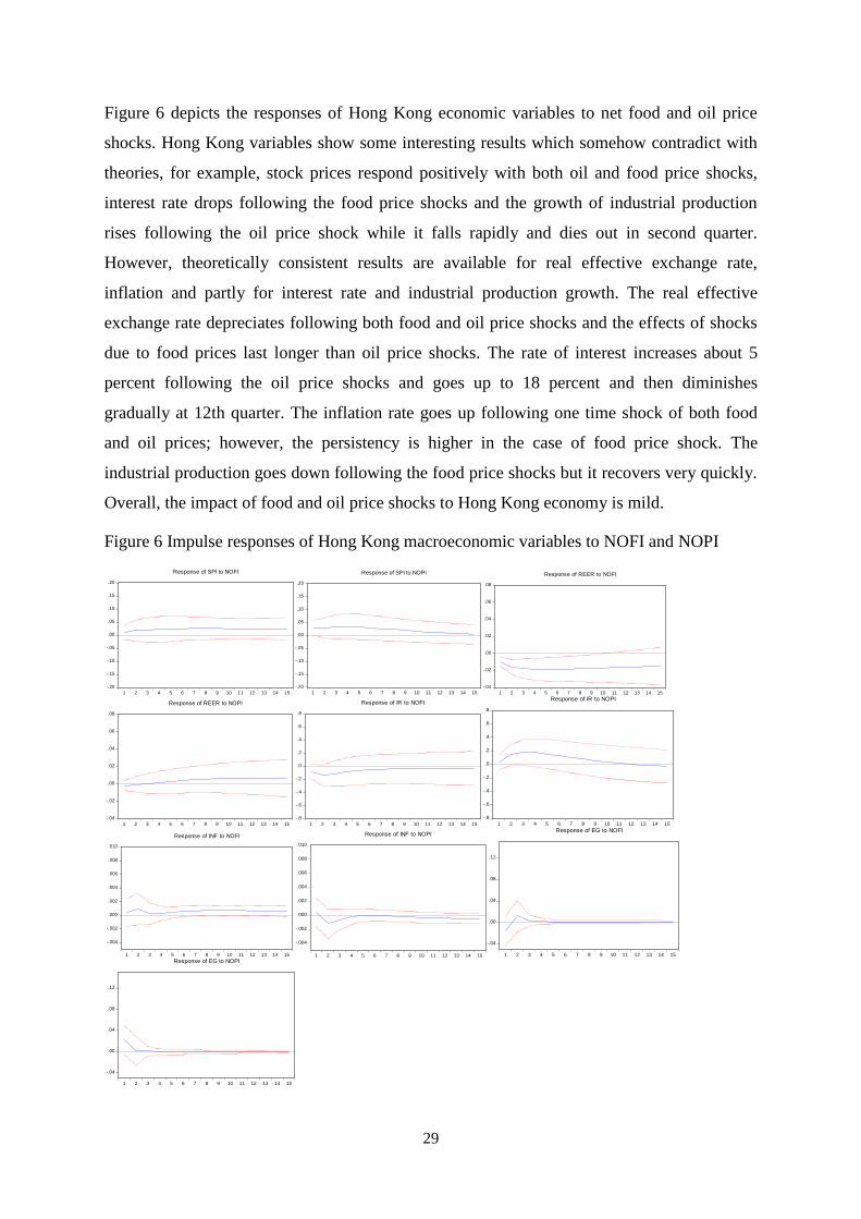
29

Figure 6 depicts the responses of Hong Kong economic variables to net food and oil price

shocks. Hong Kong variables show some interesting results which somehow contradict with

theories, for example, stock prices respond positively with both oil and food price shocks,

interest rate drops following the food price shocks and the growth of industrial production

rises following the oil price shock while it falls rapidly and dies out in second quarter.

However, theoretically consistent results are available for real effective exchange rate,

inflation and partly for interest rate and industrial production growth. The real effective

exchange rate depreciates following both food and oil price shocks and the effects of shocks

due to food prices last longer than oil price shocks. The rate of interest increases about 5

percent following the oil price shocks and goes up to 18 percent and then diminishes

gradually at 12th quarter. The inflation rate goes up following one time shock of both food

and oil prices; however, the persistency is higher in the case of food price shock. The

industrial production goes down following the food price shocks but it recovers very quickly.

Overall, the impact of food and oil price shocks to Hong Kong economy is mild.

Figure 6 Impulse responses of Hong Kong macroeconomic variables to NOFI and NOPI

-.20

-.15

-.10

-.05

.00

.05

.10

.15

.20

1 2 3 4 5 6 7 8 9 10 11 12 13 14 15

Response of SPI to NOFI

-.20

-.15

-.10

-.05

.00

.05

.10

.15

.20

1 2 3 4 5 6 7 8 9 10 11 12 13 14 15

Response of SPI to NOPI

-.04

-.02

.00

.02

.04

.06

.08

1 2 3 4 5 6 7 8 9 10 11 12 13 14 15

Response of REER to NOFI

-.04

-.02

.00

.02

.04

.06

.08

1 2 3 4 5 6 7 8 9 10 11 12 13 14 15

Response of REER to NOPI

-.8

-.6

-.4

-.2

.0

.2

.4

.6

.8

1 2 3 4 5 6 7 8 9 10 11 12 13 14 15

Response of IR to NOFI

-.8

-.6

-.4

-.2

.0

.2

.4

.6

.8

1 2 3 4 5 6 7 8 9 10 11 12 13 14 15

Response of IR to NOPI

-.004

-.002

.000

.002

.004

.006

.008

.010

1 2 3 4 5 6 7 8 9 10 11 12 13 14 15

Response of INF to NOFI

-.004

-.002

.000

.002

.004

.006

.008

.010

1 2 3 4 5 6 7 8 9 10 11 12 13 14 15

Response of INF to NOPI

-.04

.00

.04

.08

.12

1 2 3 4 5 6 7 8 9 10 11 12 13 14 15

Response of EG to NOFI

-.04

.00

.04

.08

.12

1 2 3 4 5 6 7 8 9 10 11 12 13 14 15

Response of EG to NOPI

30

Figure 7 portrays responses of Taiwan macroeconomic variables to the structural one S.D.

shock of external food and oil prices. Almost all the variables show theoretically consistent

response to the food and oil price shocks. The responses are also statistically significant in

most cases. The stock prices keep dropping until around 7 percent due to food price and 10

percent due to oil price shocks and the die out at around 7 periods. The real effective

exchange rate drops mildly with the food and oil price shocks and recovers very quickly. The

interest rate increases by 3 percent following food price shocks and sustains until the fourth

quarter while it does not show any immediate response to oil price shock, however, after

second quarter it increases by 5 percent and remains until the fourth quarter. The inflation

rate starts increasing from -20 percent following the food price shock and goes up to 20

percent at the end of third quarter and then diminishes quickly though this is not statistically

significant. And due to oil price shock it starts increasing from zero level and goes up to 20

percent and remains that high until disappears in fourth quarters. The industrial production

growth shows the highest negative impact among all other variables. It decreases sharply

following food and oil prices shocks and stays negative more than ten quarters.

Figure 7 Impulse responses of Taiwan macroeconomic variables to NOFI and NOPI

-.4

-.3

-.2

-.1

.0

.1

.2

.3

.4

1 2 3 4 5 6 7 8 9 10 11 12 13 14 15

Response of SPI to NOFI

-.4

-.3

-.2

-.1

.0

.1

.2

.3

.4

1 2 3 4 5 6 7 8 9 10 11 12 13 14 15

Response of SPI to NOPI

-.08

-.06

-.04

-.02

.00

.02

.04

.06

.08

1 2 3 4 5 6 7 8 9 10 11 12 13 14 15

Response of REER to NOFI

-.08

-.06

-.04

-.02

.00

.02

.04

.06

.08

1 2 3 4 5 6 7 8 9 10 11 12 13 14 15

Response of REER to NOPI

-2.0

-1.5

-1.0

-0.5

0.0

0.5

1.0

1.5

2.0

1 2 3 4 5 6 7 8 9 10 11 12 13 14 15

Response of IR to NOFI

-2.0

-1.5

-1.0

-0.5

0.0

0.5

1.0

1.5

2.0

1 2 3 4 5 6 7 8 9 10 11 12 13 14 15

Response of IR to NOPI

31

Figure 8 represents impulse responses of Indian macroeconomic variables to one standard

deviation structural shocks to external food and oil prices. As can be seen in Figure 9,

although in many cases the responses are not statistically significant the signs of responses

are theoretically consistent in most cases. Food price shocks show negative impacts on stock

prices, real effective exchange rate and industrial production growth and positive impacts on

interest rate and inflation. Effects of shocks to stock prices, real effective exchange rates and

inflation are mild while substantial effects can be observed in the case of interest rate and

industrial production growth. On the other hand, oil price shocks pose positive impacts to

stock prices and interest rate and negative effects to inflation and industrial growth leaving

unclear impacts on real effective exchange rate. Due to both the shocks persistent effects can

be observed in the case of real effective exchange rate and interest rates. Although real

effective exchange rate is stationary the effects of shocks do not reach to back to equilibrium

even after fifteen quarters.

Figure 8 Impulse responses of Indian macroeconomic variables to NOFI and NOPI

-4

-2

0

2

4

1 2 3 4 5 6 7 8 9 10 11 12 13 14 15

Response of INF to NOFI

-4

-2

0

2

4

1 2 3 4 5 6 7 8 9 10 11 12 13 14 15

Response of INF to NOPI

-10

-5

0

5

10

15

1 2 3 4 5 6 7 8 9 10 11 12 13 14 15

Response of EG to NOFI

-10

-5

0

5

10

15

1 2 3 4 5 6 7 8 9 10 11 12 13 14 15

Response of EG to NOPI

-.20

-.15

-.10

-.05

.00

.05

.10

.15

.20

1 2 3 4 5 6 7 8 9 10 11 12 13 14 15

Response of SPI to NOFI

-.20

-.15

-.10

-.05

.00

.05

.10

.15

.20

1 2 3 4 5 6 7 8 9 10 11 12 13 14 15

Response of SPI to NOPI

-.08

-.06

-.04

-.02

.00

.02

.04

.06

.08

1 2 3 4 5 6 7 8 9 10 11 12 13 14 15

Response of REER to NOFI

32

Figure 9 illustrates the impulse responses of selected Thai macroeconomic variables to the

structural one standard deviation shocks of food and oil prices. The effects of food and oil

price shocks are found to be statistically significant in most cases and are also statistically

significant. The stock prices respond positively with food price shock at the first quarter but

quickly after second quarter it starts declining and remains negative for a long period of time

while due to oil price shock it drops about 5 percent and remains negative until 11th quarters.

The real effective exchange rates fall by 2 percent following the food and oil price shocks and

the effects of shocks diminish in around 4 years. The interest rate is found to be more

sensitive to the food price shock. It increases more than 20 percent following the shock and

stays for a longer period. However, the effect of shocks due to oil price is rather short-lived

and the magnitudes are also lower (about 8 percent). Both food and oil price shocks put forth

inflation to up although the effects is shorter due to oil price shock. The industrial production

responds negatively following the food and oil price shocks. The effects of oil price shock

persist longer than the food price shock.

-.08

-.06

-.04

-.02

.00

.02

.04

.06

.08

1 2 3 4 5 6 7 8 9 10 11 12 13 14 15

Response of REER to NOPI

-.4

-.2

.0

.2

.4

.6

.8

1 2 3 4 5 6 7 8 9 10 11 12 13 14 15

Response of IR to NOFI

-.4

-.2

.0

.2

.4

.6

.8

1 2 3 4 5 6 7 8 9 10 11 12 13 14 15

Response of IR to NOPI

-2.0

-1.5

-1.0

-0.5

0.0

0.5

1.0

1.5

2.0

1 2 3 4 5 6 7 8 9 10 11 12 13 14 15

Response of INF to NOFI

-2.0

-1.5

-1.0

-0.5

0.0

0.5

1.0

1.5

2.0

1 2 3 4 5 6 7 8 9 10 11 12 13 14 15

Response of INF to NOPI

-4

-2

0

2

4

6

1 2 3 4 5 6 7 8 9 10 11 12 13 14 15

Response of EG to NOFI

-4

-2

0

2

4

6

1 2 3 4 5 6 7 8 9 10 11 12 13 14 15

Response of EG to NOPI

33

Figure 9 Impulse responses of Thai macroeconomic variables to NOFI and NOPI

6.4 Forecast error variance decomposition (FEVD) analysis

Table 4 shows forecast error variance decompositions for different variables in response to

the oil and food price shocks for the 1, 5, 10 and 15 quarters. Variance decompositions results

are in general supported by impulse response analysis. The stock price indices in Australia

and Singapore are found to be almost zero responsive to the food and oil price shocks. The

variation in New Zealand stock prices due to oil price shock at first quarter is only 0.14

percent while it is 2.42 percent for food price shocks. The effects of shocks gradually

increase and at the end of fifteen quarters oil price and food prices explain 13.15 and 4.70

percents of variation in stock prices respectively. In the case of Korean stock prices, the

proportion of forecast error variance due to oil price is 6.25 percent in the first period while it

is 4.22 percent for food price shocks. The proportion increases up to 11.57 percent in the 5th

-.20

-.15

-.10

-.05

.00

.05

.10

.15

.20

1 2 3 4 5 6 7 8 9 10 11 12 13 14 15

Response of SPI to NOFI

-.20

-.15

-.10

-.05

.00

.05

.10

.15

.20

1 2 3 4 5 6 7 8 9 10 11 12 13 14 15

Response of SPI to NOPI

-.04

-.03

-.02

-.01

.00

.01

.02

.03

.04

1 2 3 4 5 6 7 8 9 10 11 12 13 14 15

Response of REER to NOFI

-.04

-.03

-.02

-.01

.00

.01

.02

.03

.04

1 2 3 4 5 6 7 8 9 10 11 12 13 14 15

Response of REER to NOPI

-.8

-.6

-.4

-.2

.0

.2

.4

.6

.8

1 2 3 4 5 6 7 8 9 10 11 12 13 14 15

Response of IR to NOFI

-.8

-.6

-.4

-.2

.0

.2

.4

.6

.8

1 2 3 4 5 6 7 8 9 10 11 12 13 14 15

Response of IR to NOPI

-.004

-.002

.000

.002

.004

.006

.008

.010

.012

1 2 3 4 5 6 7 8 9 10 11 12 13 14 15

Response of INF to NOFI

-.004

-.002

.000

.002

.004

.006

.008

.010

.012

1 2 3 4 5 6 7 8 9 10 11 12 13 14 15

Response of INF to NOPI

-.04

-.03

-.02

-.01

.00

.01

.02

.03

.04

1 2 3 4 5 6 7 8 9 10 11 12 13 14 15

Response of EG to NOFI

-.04

-.03

-.02

-.01

.00

.01

.02

.03

.04

1 2 3 4 5 6 7 8 9 10 11 12 13 14 15

Response of EG to NOPI

34

quarter for oil prices and then declines gradually and for food prices it decrease after the first

quarter. The oil price shock contributes 7.50 percent variation to Hong Kong stock prices at

the first period and then gradually declines while the contribution of food price shock is only

0.64 percent at the first period and reaches up to 6.80 percent at the end of fifteen quarters. In

Taiwan, the contribution of oil price shocks to stock prices is only 0.03 percent at the first

period while contribution of food price shock is 7.78 percent. The proportions increase until

5th quarter (44.76 percent) for oil prices and until 10th quarter (19.60 percent) for food

prices. The contribution of oil price shock to Indian stock prices is marginal, only 1.87

percent at the first period and then declines gradually. And the contribution of food prices

starts from 1.48 percent at the first quarter and increases up to 17 percent at the end of 15

quarters. Oil price shocks have substantial contribution to the variation of stock prices in

Thailand while the contribution of food price shock is marginal at the first period. However,

at the end of 15 quarters the contributions of both the price shocks are more than 10 percent.

The oil and food price shocks substantially contribute to the variation of real effective

exchange rate in each country excepting Singapore. Although the contribution of oil price

shock to Australian exchange rate is 0.07 percent at the first quarter it increases substantially

during subsequent periods reaching highest as 15 percent at 15th quarter. Food price shock

contributes to the variation of Australian exchange rate by 7.64 percent at the first quarter;

reaches up to 11.21 percent at the 5th quarter and then decreases gradually. The oil and food

price shocks explain 3.87 and 8.96 percents of the variation of New Zealand real effective

exchange rate at the first quarter of the shock and then proportions increase gradually up to

10th quarter before starts falling. The shares of oil and food price shocks to the variation of

Korean real effective exchange rate are 9.42 and 6.82 percents respectively at the first period

and then keep rising. In Hong Kong, in the variation of real exchange rate the oil price shocks

have marginal contribution (0.73 percent); however, the contribution of food price shock is

noticeable (16.68 percent) at the first quarter. The ratio of oil and food price shocks in the

variation of Taiwanese real effective exchange rate are 4.81 and 11.82 percents respectively

at the first quarter while these keep rising until the 10th quarter. Although oil price shock has

almost zero percentage share to the variation of Indian real effective exchange rate, the

contribution of food prices are not ignorable. The contribution of food price shocks is 0.22

percent following the shock while it increases up to 10.32 percent at the end of 15 quarter.

The oil and food price shocks contribute 23.48 and 19.48 percents to the variation of Thai

35

real effective exchange rate respectively at the first period keep substantial contributions at

the subsequent periods.

Interest rates in Australia and Singapore are found to be insignificantly responsive to the

oil and food price shocks. The variation in interest rate due to oil and food price shocks is less

than 1 percent in both cases even after 15 quarters. The contribution of oil and food prices to

the variation of interest rates is observed to be higher in Korea, Taiwan and Thailand ranging

from more than 5 percent to 28 percent at 15th quarter. The contribution of food price shocks

as proportion to the variation in interest rate in New Zealand, Hong Kong and India seem to

be lower than the contribution of oil price shocks.

The variance decompositions for inflation show that in the variation of the Singaporean

and Indian inflation rates the contribution of oil and food price shocks are negligible (around

1 percent). In Australia the contribution of oil price shock to the variation of inflation is 4.35

percent following the shock at the first quarter and then diminish gradually while contribution

of food price shocks seem to be insubstantial. The New Zealand inflation varies 2.34 and 0.54

percents due to oil and food price shocks respectively at the first quarter and then the effects

keep increasing until the 15th quarter. The role of oil and food price shocks to the variation of

Korean inflation is 1.43 and 0.89 percents respectively at the first quarter while the

proportions increase in subsequent quarters. Although the contribution of oil and food prices

to the variation of Hong Kong inflation is less than 1 percent at the first quarter the

proportions increase more up to more than 3 percent at the 15th quarter. The Taiwan inflation

seems to be most sensitive to both oil and food price shocks. The contribution of oil and food

prices is 18.33 and 14.97 percents respectively during the 15th quarter. The variation of Thai

inflation is found to be highly explained by oil and food price shocks at the first quarter

(11.58 and 4.79 percents) and the proportions go up to more than 12 percent at the 15th

quarter.

In terms of the industrial production growth, the contribution of oil and food price shock is

mild for Australia, New Zealand, Singapore and India. Like many other variables, the role of

oil and food price shocks to the variation of industrial growth can be observed for Korea,

Hong Kong, Taiwan, and Thailand. Although the proportions of oil and food price shocks in

the variability of industrial growth for Korea and Thailand are low at the first quarter, they

increase in the subsequent quarters while significant contributions are viewed in Hong Kong

and Taiwan following the shock in the first quarter.

36

Table 5 Forecast error variance decompositions

Variables Horizon AUS NZ KOR SIN HK TWN IN TH

NOPI NOFI NOPI NOFI NOPI NOFI NOPI NOFI NOPI NOFI NOPI NOFI NOPI NOFI NOPI NOFI

SPI

1 0.01 1.19 0.14 2.42 6.25 4.22 0.14 0.12 7.50 0.64 0.03 7.78 1.87 1.48 3.23 0.20

5 0.60 1.69 7.43 3.29 11.57 3.75 0.04 0.65 8.20 2.78 44.76 15.87 0.47 11.67 17.97 1.10

10 0.45 0.99 11.82 4.65 8.46 2.64 0.05 0.83 8.27 5.17 42.31 19.60 0.51 15.55 16.98 7.60

15 0.99 0.88 13.15 4.70 6.69 2.65 0.07 0.86 7.37 6.80 27.07 13.76 0.78 17.05 14.93 11.48

REER

1 0.07 7.64 3.87 8.96 9.42 6.82 0.00 2.23 0.73 16.68 4.81 11.82 0.07 0.22 23.48 19.48

5 11.22 11.21 15.35 29.61 33.63 28.35 0.92 0.87 0.30 31.47 29.41 11.51 0.08 7.05 16.50 19.98

10 13.91 10.58 15.68 29.76 34.55 29.49 0.71 0.96 1.63 28.44 32.96 22.92 0.10 9.32 16.69 19.51

15 14.60 10.34 15.77 29.16 34.82 29.98 0.56 1.09 2.15 22.73 21.76 18.07 0.12 10.76 16.55 19.76

IR

1 0.93 0.36 2.42 0.08 0.36 5.06 0.93 0.71 0.49 3.08 1.66 8.10 0.44 0.32 2.22 12.52

5 0.60 0.08 3.24 0.06 10.88 28.11 0.41 0.36 9.08 4.34 8.88 2.75 3.01 2.31 1.70 32.74

10 0.48 0.21 2.39 0.69 8.86 17.94 0.35 0.33 6.24 2.58 20.68 8.87 3.54 2.67 2.40 32.48

15 0.86 0.48 2.07 1.63 12.93 15.33 0.36 0.33 4.44 1.96 23.35 19.78 3.56 2.79 5.15 28.33

INF

1 4.35 0.17 2.34 0.54 1.43 0.89 0.27 1.01 0.21 0.25 0.52 7.87 0.98 0.34 11.58 4.79

5 3.79 0.35 7.35 1.45 8.35 9.90 0.69 1.23 2.25 1.45 37.37 18.29 1.03 0.97 11.94 12.41

10 3.66 0.39 7.07 1.50 9.66 10.46 0.70 1.14 2.24 3.52 34.90 24.77 1.06 1.07 12.25 12.17

15 3.69 0.46 6.98 1.69 10.51 10.95 0.69 1.11 3.00 5.26 18.33 14.97 1.05 1.26 12.29 12.20

EG

1 1.73 0.94 0.20 0.70 1.43 0.31 0.18 1.06 3.69 1.99 62.33 14.49 0.32 0.21 0.00 3.21

5 1.69 1.09 1.72 1.41 6.32 4.73 0.25 2.35 3.59 3.10 41.46 25.30 0.33 3.07 14.76 3.96

10 1.69 1.09 1.72 1.47 6.40 4.76 0.25 2.34 3.62 3.12 34.91 22.68 0.32 3.08 15.60 3.78

15 1.69 1.09 1.82 1.63 6.45 4.79 0.25 2.34 3.63 3.13 24.71 15.40 0.33 3.08 15.59 4.13

7. Discussion, policy implications and limitation

The empirical results of this study reasonably reflect the background characteristics of

economies covered by the study. The Australian and New Zealand economies are found less

affected by international oil and food price shocks. The channel which found to be significant

for these two countries is real effective exchange rate. In both countries the exchange rates

depreciate followed by oil and food price shocks. Although Australia and New Zealand have

little amount of proven oil reserve, these two countries possess a number of other mineral

resources which dominate the energy sector, for example, According to IEA, in 2008

Australia produces 99 percent of electricity by using different fuels including coal as major

(76 percent) and only 1 percent electricity comes from oil. In 2008, New Zealand produces

99.97 percent electricity from other sources than oil out of which 75 percent comes from

hydro and gas plants. Only 0.03 percent is produced using oil as fuel. The main uses of oil in

these countries are for transportation. Industrial production indices do not include transport

cost directly and that could be one possible reason that industrial production are found to be

not responsive to oil price shocks. The reasons for which industrial production are not

affected by oil price shocks are also applicable for stock prices. These alternative mineral

resources help Australia to accommodate oil supply shocks. Both of these countries maintain

37

inflation targeting monetary policy which could be the reason to accommodate the oil price

shock through inflation and interest rate. Because of being net food exporters in the world

market Australia and New Zealand economy are not adversely affected by food price shocks.

The depreciation of exchange rate following oil and food price shocks should not be taken as

adverse for these countries because it may increase the demand for export goods.

The four Asian tiger economies are found to behave mainly in two ways to oil and food

price shocks. Korea and Taiwan specialized in manufacturing and information technology are

found to be much affected by oil and food price shocks while Singapore and Hong Kong

specialized in international financial services are found not affected. Korea being a resource

poor country is most vulnerable to oil and food price shocks. Korea is fifth in the top net

importers list of oil and third in the list of top consumers as non oil producing countries after

Japan and Germany. The findings related to oil price shock on macroeconomic variables of

Korea is consistent with Cuňado and Gracia (2003) and Hsieh (2008). Possible interpretation

can be as follows. Heavy industries in Korea are also dependent on the electricity generated

mostly by imported oil. Because of this dependency on oil, oil price increase badly affects

industrial output. When industrial output decreases inflation may rise. Because of the

increased money demand for importation of oil the domestic interest rate increases. Korea

also needs to import most of the food products which obviously put negative impacts to

import bills and thus to the other macroeconomic variables. Taiwan has the similar economic

characteristics as of Korea. The reasons why Korean output and other variables are impacted

by oil price shocks are also applicable to Taiwan case. However, Taiwan is found to be more

accommodative to food price shocks. The major channel through which food price shocks

transmit to Taiwan economy is real exchange rate. Since Taiwan does not import much food

products the effects of food price shocks are not that severe as oil price is. Singapore and

Hong Kong economies are dependent in financial services and financial services are not

much dependent on oil like industrial productions. That might be possible reasons that these

countries are not much affected by oil price shocks. In Singapore case, selected variables are

found not responsive to either oil or food price shocks which is partly consistent with Chang

and Wong (2003) and Cuňado and Gracia (2003). Chang and Wong (2003) report that oil

price has marginal impact on GDP, CPI and unemployment rate in Singapore. However,

Cuňado and Gracia (2003) show that there is no causal relationship between oil price and

Singaporean economic growth although they document evidence of causal relationship

between oil price and inflation. In Hong Kong oil price shocks found to be transmit through

38

interest rate channel while other variables are not significantly responsive to the oil price

shock which is consistent to Ran et al.(2010). The reason could be the increase of money

demand due to excess expenditure on imported oil. In terms of food price shock, exchange

rate is found as the channel to be transmitted. Hong Kong lacks of arable land which forced it

to import all of its food products needed. Because of this reason there must be pressure on

import bills which help Hong Kong dollar to be depreciated.

In Indian case, food prices have dominant impact on the macroeconomic variables than oil

prices. The major channel through which oil price shock transmits to Indian economy is

interest rate derived from money demand for importing oil. India has proven reserve of oil to

meet 25 percent of domestic demands and also has coal and other mineral resources which

are used for generating energy in the country. India meets most of its domestic energy

demand through its coal reserves. Because of these reasons, manufacturing output is not

dependent on the imported oil. This could be one of reasons that Indian industrial productions

are not affected by oil price shocks although this findings contradict to Managi and Kumar

(2009). However, due to food price hike the labour forces in the industrial sector may

demand higher wages and thus demand for labour decreases which decreases output in the

industrial sector. Once output decreases the stock price also decreases. However, the situation

improves rapidly because of exchange rate depreciation.

Although there is lack of evidence of Granger causality, impulse response and variance

decompositions functions in the sense of statistical significance suggest that Thai

macroeconomic variables such as stock prices, real effective exchange rates and industrial

output are found to be adversely affected by oil price shock which is consistent to Rafiq et al.

(2009). On the other hand, real effective exchange rate, interest rate and inflation are found to

be adversely affected by food price shocks. Although Thailand uses natural gas mostly for

generating energy the demand for oil is also high. Since industrial outputs hampers, the stock

prices decrease. Real effective exchange rates are on pressure because of excess import bill

due to oil price increase. And because of global food price increase, the demand for Thai food

might decrease. The export earning decreases that helps exchange rates to depreciate. As net

export falls it may increase inflation. The adverse effect of food prices on inflation in

Thailand is consistent to Galesi and Lombardi (2009a). They state that developing countries

price levels are much affected by food prices than oil price shocks.

Overall, the empirical results suggest that the resource poor countries specialized in the

production of heavy manufacturing industries dependent on oil like Korea are Taiwan are

39

most vulnerable to oil price shocks. These countries may adopt different conservatory

measures and switch to renewable energy sectors to cope with oil price shocks. Countries like

Australia and New Zealand which have diverse mineral resources other than oil are better in

coping oil price shocks. The only adverse effects these countries get the depreciation of local

currency which, in other words, is good for their export sector. Developed countries which

specialized in financial services such as Singapore and Hong Kong are accommodative of oil

price shocks. Developing countries specialized both in primary and manufacturing products

like India with diverse mineral resources are also not vulnerable to oil price shocks. However,

Thailand the case of Thailand is different. Although it possesses huge amount of natural gas

its industrial output are affected by oil price shock and also being major exporter food the

economy is negatively exposed to external food price shocks. Thailand thus need external

shocks accommodative policies along with enhance of using alternative sources of energy.

As mentioned earlier, we use selected macroeconomic and financial variables and interpret

results based on the findings in regards to the selected variables. The impact of both oil and

food prices could be different if we would have used GDP data instead of industrial

production and also would include government or private expenditure data. The results could

also be different if terms of trade and trade balance data were used. Therefore, when take the

findings for implications this limitation should be taken into consideration. The study can be

extended to over identified structural VAR model.

8. Conclusions

The objective of this study was to investigate the effects of world oil and food price

shocks to selected macroeconomic variables of Australia, New Zealand, Korea, Singapore,

Hong Kong, Taiwan, India, and Thailand. By employing structural vector autoregressive

(SVAR) models, the study reveals that resource poor countries that specialize in heavy

manufacturing industries like Korea and Taiwan are mostly affected by international oil price

shocks. Increase in oil prices reduces the growth of industrial production, real effective

exchange rate and stock prices and increases inflation and interest rates in these countries. On

the other hand, oil poor nations such as Australia and New Zealand with diverse mineral

resources other than oil are not affected much by oil price shocks. The only channel which is

affected by price shocks in these two countries is real effective exchange rates. Increase in oil

and food prices help depreciating exchange rates in these countries. Countries which are oil

poor but specialized in international financial services such as Singapore and Hong Kong are

40

also not affected by oil price shocks. Developing countries with diverse natural resources

with limited reserve of oil e.g., India is negligibly affected by oil price shocks. Indian interest

rate show positive response to oil price shocks. In contrast, Thailand being resource rich

country other than oil is not accommodative of oil price shocks. Thai stock prices, stock

prices and industrial production growth respond negatively to the oil price shocks while oil

price increase has positive influence on inflation and interest rate. Industrial outputs of food

exporter countries like Australia, New Zealand, and Thailand are not affected by global food

price shocks. However, output of India is adversely affected by global food price shocks.

Among food importer countries except Korea other countries’ output are also not adversely

affected by food price shocks. Increases food prices help depreciation of exchange rates in

almost all countries except Singapore. The evidence of effects of food prices on stock prices

are almost nil except India. Positive pressure of food prices on inflation and interest rate are

found for Korea and Thailand only. The findings suggest that Korea, Taiwan and Thailand

may design effective policy measures to cope with oil price shocks. Renewable energy

sources could be one of the options for these countries to accommodate oil price shocks.

Food reserve increase and enhanced local production can help countries to cope with food

price shocks.

REFERENCES

Abott, P.C., Hurt, C. & Tyner, W.E., 2009. What's driving food prices? Farm foundation issue report.

Akram, Q.F., 2004. Oil prices and exchange rates: Norwegian evidence. Econometrics Journal, 7 (2), 476-504.

Aksoy, M.A. & Ng, F., 2008. Who are the net food importing countries? : The World Bank, Policy Research

Working Paper Series: 4457.

Aleisa, E.A. & Dibooglu, S., 2002. Sources of real exchange rate movements in saudi arabia. Journal of

Economics and Finance, 26 (1), 101-110.

Amano, R.A. & Van Norden, S., 1998. Oil prices and the rise and fall of the us real exchange rate. Journal of

International Money and Finance, 17 (2), 299-316.

Amisano, G. & Giannini, C., 1997. Topics in structural var econometrics Berlin: Springer-Verlag.

Andreopoulos, S., 2009. Oil matters: Real input prices and u.S. Unemployment revisited. B.E. Journal of

Macroeconomics: Topics in Macroeconomics, 9 (1).

Apergis, N. & Miller, S.M., 2009. Do structural oil shocks affect stock prices. Working paper, University of

Nevada, Las Vegas, Department of Economics, 0917.

Balke, N.S., Brown, S.P.A. & Yucel, M.K., 2002. Oil price shocks and the u.S. Economy: Where does the

asymmetry originate? Energy Journal, 23 (3), 27-52.

Basher, S.A. & Sadorsky, P., 2006. Oil price risk and emerging stock markets. Global Finance Journal, 17 (2),

224-251.

Benassy-Quere, A., Mignon, V. & Penot, A., 2005. China and the relationship between the oil price and the

dollar. CEPII research center, Working Papers.

Bernanke, B.S., Gertler, M. & Watson, M., 1997. Systematic monetary policy and the effects of oil price shocks.

Brookings Papers on Economic Activity, (1), 91-142.

Bernanke, B.S., Gertler, M. & Watson, M.W., 2004. Oil shocks and aggregate macroeconomic behavior: The

role of monetary policy: Reply. Journal of Money, Credit, and Banking, 36 (2), 287-291.

41

Bjornland, H.C., 2000. The dynamic effects of aggregate demand, supply and oil price shocks- a comparative

study. The Mancheter School, 68 (5), 578-607.

Blanchard, O.J. & Gali, J., 2007. The macroeconomic effects of oil price shocks: Why are the 2000s so different

from the 1970s? : Department of Economics and Business, Universitat Pompeu Fabra, Economics

Working Papers.

Bohi, D.R., 1991. On the macroeconomic effects of energy price shocks. Resources and Energy, 13 (2), 145-

162.

Breitenfeller, A. & Cuaresma, J.C., 2008. Crude oil prices and usd/eur exchange rate. Monetary Policy and the

Economy, Q4/08 (102-121).

Breitung, J., Bruggemann, R. & Lutkepohl, H., 2004. Applied time series econometrics West Nyack, NY, USA:

Cambridge University Press.

Brown, S.P.A. & Phillips, K.R., 1986. Exchange rates and world oil prices. Federal Reserve Bank of Dallas

Economic Review, 1-10.

Brown, S.P.A. & Yucel, M.K., 2002. Energy prices and aggreagte economic activity: An interpretative survey.

Quarterly Review of Economics and Finance, 42, 193-208.

Burbidge, J. & Harrison, A., 1984. Testing for the effects of oil-price rises using vector autoregressions.

International Economic Review, 25 (2), 459-484.

Carruth, A.A., Hooker, M.A. & Oswald, A.J., 1998. Unemployment equilibria and input prices: Theory and

evidence from the united states. Review of Economics and Statistics, 80 (4), 621-628.

Chang, Y. & Wong, J.F., 2003. Oil price fluctuation and singapore economy. Energy Policy, 31, 1151-1165.

Chen, N.-F., Roll, R., Ross, S.A. & Lo, A.W., 2007. Economic forces and the stock market. Static asset-pricing

models. Elgar Reference Collection. International Library of Financial Econometrics series, vol. 2.

Cheltenham, U.K. and Northampton, Mass.: Elgar, 365-385.

Cologni, A. & Manera, M., 2009. The asymmetric effects of oil shocks on output growth: A markov-switching

analysis for the g-7 countries. Economic Modelling, 26 (1), 1-29.

Cong, R.-G., Wei, Y.-M., Jiao, J.-L. & Fan, Y., 2008. Relationships between oil price shocks and stock market:

An empirical analysis from china. Energy Policy, 36 (9), 3544-3553.

Cooper, R.L., 1994. Changes in exchange rates and oil prices for saudi arabia and other opec member countries.

The journal of energy and development, 20 (1), 109-128.

Cuňado, J. & Gracia, F.P., 2003. Do oil price shocks matter? Evidence for some european countries. Energy

Economics, 25, 137-154.

Cunado, J. & Perez De Gracia, F., 2005. Oil prices, economic activity and inflation: Evidence for some asian

countries. Quarterly Review of Economics and Finance, 45 (1), 65-83.

Davis, S.J. & Haltiwanger, J., 2001. Sectoral job creation and destruction responses to oil price changes. Journal

of Monetary Economics, 48 (3), 465-512.

Davis, S.J., Loungani, P. & Mahidhara, R., 1997. Regional labour fluctuations: Oil shocks, military spending

and other driving forces. Board governors of the Federal Reserve System international finance

discussion paper, No. 578.

Dickey, D.A. & Fuller, W.A., 1979. Distribution of the estimates for autoregressive time series with a unit root.

Journal of the American Statistical Association, 74, 427-431.

Faff, R.W. & Brailsford, T.J., 1999. Oil price risk and the australian stock market. Journal of Energy Finance &

Development, 4 (1), 69-87.

Farzanegan, M.R., 2009. The effects of oil price shocks on the iranian economy. Energy Economics, 31, 134-

151.

Ferderer, J.P., 1996. Oil price volatility and the macroeconomy: A solution of the asymmetry puzzle. Journal of

macroeconomics, 18 (1), 1-26.

Finn, M.G., 2000. Perfect competition and the effects of energy price increases on economic activity. Journal of

Money, Credit and banking 32 (3), 400-416.

Francesco, G., 2009. The economic effects of oil price shocks on the uk manufacturing and services sector.

MPRA, paper no. 16171.

Galesi, A. & Lombardi, M.J., 2009a. External shocks and interantional inflation linkages: A global var analysis.

European central bank, WP. 1062.

Galesi, A. & Lombardi, M.J., 2009b. External shocks and international inflation linkages: A global var analysis.

European Central Bank, Working Paper Series: 1062, 45 pages.

Gil-Alana, L.A., 2003. Unemployment and real oil prices in australia: A fractionally cointegrated approach.

Applied Economics Letters, 10 (4), 201-204.

Gisser, M. & Goodwin, H.T., 1986. Crude oil and macroeconomy: Tests for some popular notions. Journal of

Money, Credit and Banking, 18, 95-103.

42

Gounder, R. & Bartlett, M., 2007. Oil price shocks and economic growth: Evidence for new zealand, 1989-

2006. Paper presented at the New Zealand Association of Economist Annual Conference, Christchurch

27-29 June 2007.

Hakro, A.N. & Omezzine, A.M., 2010. Macroeconomic effects of oil and food price shocks to the oman

economy. Middle Eastern Finance and Economics, (6), 72-90.

Hamilton, J.D., 1983. Oil and the macroeconomy since world war ii. Journal of Political Economy, 91 (2), 228-

248.

Hamilton, J.D., 1988. A neoclassical model of unemployment and business cycles. Journal of Political

Economy, 96, 593-617.

Hamilton, J.D., 1996. This is what happened to the oil price-macroeconomy relationship. Journal of Monetary

Economics, 38 (2), 215-220.

Hamilton, J.D., 2003. What is an oil shock? Journal of Econometrics, 113 (2), 363-398.

Hamilton, J.D., 2010. Nonlinearities and the macroeconomic effects of oil prices. National Bureau of Economic

Research, Inc, NBER Working Papers: 16186.

Hamilton, J.D. & Herrera, A.M., 2004. Oil shocks and aggregate macroeconomic behavior: The role of

monetary policy: Comment. Journal of Money, Credit, and Banking, 36 (2), 265-286.

Headey, D. & Fan, S., 2008. Anatomy of a crisis: The causes and consequences of surging food prices.

Agricultural Economics, 39, 375-391.

Hooker, M.A., 1996. What happened to the oil price-macroeconomy relationship? Journal of Monetary

Economics, 38 (2), 195-213.

Hsieh, W.-J., 2008. Effects of oil price shocks and macroeconomic conditions on output fluctuations for korea.

Journal of International and Global Economic Studies, 1 (2), 84-91.

Huang, B.-N., Hwang, M.J. & Peng, H.-P., 2005. The asymmetry of the impact of oil price shocks on economic

activities: An application of the multivariate threshold model. Energy Economics, 27 (3), 455-476.

Huang, R.D., Masulis, R.W. & Stoll, H.R., 1996. Energy shocks and financial markets. Journal of Futures

Markets, 16 (1), 1-27.

Iwayemi, A. & Fowowe, B., 2011. Impacts of oil price shocks on selected macroeconomic variables in nigeria.

Energy Policy, 39, 603-612.

Jones, C.M. & Kaul, G., 1996. Oil and stock markets. The Journal of Finance, 51 (2), 463-491.

Keane, M.P. & Prasad, E.S., 1996. The employment and wage effects of oil price chnages: A sectoral analysis.

Review of Economics and Statistics, 78 (3), 389-400.

Kilian, L. & Vigfussion, R.J., 2009. Pitfalls in estimating asymmetric effects of energy price shocks. CEPR

Discussion Paper No. 7284.

Lardic, S. & Mignon, V., 2008. Oil prices and economic activity: An asymmetric cointegration approach.

Energy Economics, 30 (3), 847-855.

Lee, J. & Strazicich, M., 2003. Minimum lm unit root test with two structual breaks. Review of Economics and

Statistics, 63, 1082-1089.

Lee, K. & Ni, S., 2002. On the dynamic effects of oil price shocks: A study using industry level data. Journal of

Monetary Economics, 49 (4), 823-852.

Lee, K., Ni, S. & Ratti, R.A., 1995. Oil shocks and the macroeconomy: The role of price variability. Energy

Journal, 16 (4), 39-56.

Lee, S.J., 2009. Volatility spillover effects among six asian countries. Applied Economics Letters, 16 (4-6), 501-

508.

Lescaroux, F., 2011. The oil price-microeconomy relationship is alive and well. Energy Journal, 32 (1), 25-47.

Lescaroux, F. & Mignon, V., 2009. The symposium on 'china's impact on the global economy': Measuring the

effects of oil prices on china's economy: A factor-augmented vector autoregressive approach. Pacific

Economic Review, 14 (3), 410-425.

Lippi, F. & Nobili, A., 2009. Oil and the macroeconomy: A quantitative structural analysis. Bank of Italy

working paper, No. 704.

Lizardo, R.A. & Mollick, A.V., 2010. Oil price fluctuations and u.S. Dollar exchange rates. Energy Economics,

32 (2), 399-408.

Lumsdaine, R. & Papell, D., 1997. Multiple trend breaksand the unit root hypothesis. Review of Economics and

Statistics, 79, 212-218.

Managi, S. & Kumar, S., 2009. Macroeconomic effects of oil price shocks. The economics of sustainable

development. 32 ed.: Springer New York, 221-243.

Mork, K.A., 1989. Oil and macroeconomy when prices go up and down: An extension of hamilton's results.

Journal of Political Economy, 97 (3), 740-744.

Papapetrou, E., 2001. Oil price shocks, stock market, economic activity and employment in greece. Energy

Economics, 23 (5), 511-532.

43

Park, J. & Ratti, R.A., 2008. Oil price shocks and stock markets in the u.S. And 13 european countries. Energy

Economics, 30 (5), 2587-2608.

Phillips, P.C.B. & Perron, P., 1987. Testing for a unit root in time series regression. Cowles Foundation, Yale

University, Cowles Foundation Discussion Papers: 795R, 31 pages.

Rafiq, S., Salim, R. & Bloch, H., 2009. Impact of crude oil price volatility on economic activities: An empirical

investigation in the thai economy. Resources Policy, 34 (3), 121-132.

Ran, J., Voon, J.P. & Li, G., 2010. How do oil price shocks affect a small non-oil producing economy?

Evidence from hong kong. Pacific Economic Review, 15 (2), 263-280.

Raymond, J.E. & Rich, R.W., 1997. Oil and the macroeconomy: A markov state-switching approach. Journal of

Money, Credit, and Banking, 29 (2), 193-213.

Rotemberg, J.J. & Woodford, M., 1996. Imperfect competition and the effects of energy prices increases on

economic activity. Journal of Money, Credit and Banking, 1 (28(4)), 549-577.

Sadorsky, P., 1999. Oil price shocks and stock market activity. Energy Economics, 21 (5), 449-469.

Sadorsky, P., 2003. The macroeconomic determinants of technology stock price volatility. Review of Financial

Economics, 12 (2), 191-205.

Segal, P., 2007. Why do oil price shocks no longer shock? Oxford Institute of Energy Studies, Working Paper

No. 35.

Sims, C.A., 1980. Macroeconomics and reality. Econometrica, 48 (1), 1-48.

Tang, W., Wu, L. & Zhang, Z., 2010. Oil price shocks and their short- and long-term effects on the chinese

economy. Energy Economics, 32 (1), S3-14.

Valadkhani, A. & Mitchell, W.F., 2002. Assessing the impact of changes in petroleum prices on inflation and

household expenditures in australia. Australian Economic Review, 35 (2), 122-132.

Von Braun, J., 2008. Rising food prices: What should be done? EuroChoices, 7 (2), 30-35.

Yousefi, A. & Wirjanto, T.S., 2004. The empirical role of the exchange rate on the crude-oil price formation.

Energy Economics, 26 (5), 783-799.

Zhang, Q. & Reed, M., 2008. Examining the impact of the world crude oil prices on china's agricultural

commodity prices: The case of corn, soybean and pork The Southern Agricultural Economics

Association Annual Meetings, Dallas, TX, February 2-5, 2008.

Zhang, Y.-J., Fan, Y., Tsai, H.-T. & Wei, Y.-M., 2008. Spillover effect of us dollar exchange rate on oil prices.

Journal of Policy Modeling, 30 (6), 973-991.