economic bulletin - december 2017 - banco de portugal · economic bulletin | december 2017 ......

Economic BulletinDecember 2017

Economic Bulletin December 2017

Lisbon, 2017 • www.bportugal.pt

Economic Bulletin | December 2017 • Banco de Portugal Av. Almirante Reis, 71 | 1150-012 Lisboa • www.bportugal.pt

• Edition Economics and Research Department • Design and printing Communication and Museum Department | Publishing

and Image Unit • Print run 25 • ISSN 0872-9794 (print) • ISSN 2182-0368 (online) • Legal Deposit no. 241772/06

ContentsProjections for the Portuguese economy 2017-2020

Box 1 | Projection assumptions | 14

Box 2 | The import content of global demand in Portugal | 28

Box 3 | Effect of an interest rate rise on household income: heterogeneity by age class and income quartiles | 32

Box 4 | Macroeconomic impact of the crisis in Catalonia | 34

Special issue

Potential output: challenges and uncertainties | 39

Box 1 | The Cobb-Douglas production function | 42

Box 2 | The Phillips curve | 45

Box 3 | Okun’s law | 47

Box 4 | Potential output revisions | 58

Projections for the Portuguese economy 2017-2020

Box 1 | Projection assumptions

Box 2 | The import content of global demand in Portugal

Box 3 | Effect of an interest rate rise on household income: heterogeneity by age class and income quartiles

Box 4 | Macroeconomic impact of the crisis in Catalonia

7Projections for the Portuguese economy 2017-2020

1. Projections for the Portuguese economy 2017-20201

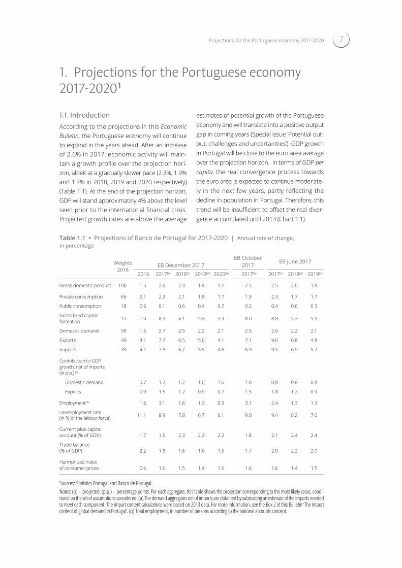
1.1. IntroductionAccording to the projections in this Economic Bulletin, the Portuguese economy will continue to expand in the years ahead. After an increase of 2.6% in 2017, economic activity will main-tain a growth profile over the projection hori-zon, albeit at a gradually slower pace (2.3%, 1.9% and 1.7% in 2018, 2019 and 2020 respectively) (Table 1.1). At the end of the projection horizon, GDP will stand approximately 4% above the level seen prior to the international financial crisis. Projected growth rates are above the average

estimates of potential growth of the Portuguese economy and will translate into a positive output gap in coming years (Special issue ‘Potential out-put: challenges and uncertainties’). GDP growth in Portugal will be close to the euro area average over the projection horizon. In terms of GDP per capita, the real convergence process towards the euro area is expected to continue moderate-ly in the next few years, partly reflecting the decline in population in Portugal. Therefore, this trend will be insufficient to offset the real diver-gence accumulated until 2013 (Chart 1.1).

Table 1.1 • Projections of Banco de Portugal for 2017-2020 | Annual rate of change, in percentage

Weights 2016

EB December 2017EB October

2017EB June 2017

2016 2017(p) 2018(p) 2019(p) 2020(p) 2017(p) 2017(p) 2018(p) 2019(p)

Gross domestic product 100 1.5 2.6 2.3 1.9 1.7 2.5 2.5 2.0 1.8

Private consumption 66 2.1 2.2 2.1 1.8 1.7 1.9 2.3 1.7 1.7

Public consumption 18 0.6 0.1 0.6 0.4 0.2 0.3 0.4 0.6 0.3

Gross fixed capital formation 15 1.6 8.3 6.1 5.9 5.4 8.0 8.8 5.3 5.5

Domestic demand 99 1.6 2.7 2.5 2.2 2.1 2.5 2.6 2.2 2.1

Exports 40 4.1 7.7 6.5 5.0 4.1 7.1 9.6 6.8 4.8

Imports 39 4.1 7.5 6.7 5.5 4.8 6.9 9.5 6.9 5.2

Contribution to GDP growth, net of imports (in p.p.) (a)

Domestic demand 0.7 1.2 1.2 1.0 1.0 1.0 0.8 0.8 0.8

Exports 0.9 1.5 1.2 0.9 0.7 1.5 1.8 1.2 0.9

Employment (b) 1.6 3.1 1.6 1.3 0.9 3.1 2.4 1.3 1.3

Unemployment rate (in % of the labour force) 11.1 8.9 7.8 6.7 6.1 9.0 9.4 8.2 7.0

Current plus capital account (% of GDP) 1.7 1.5 2.3 2.2 2.2 1.8 2.1 2.4 2.4

Trade balance (% of GDP) 2.2 1.8 1.6 1.6 1.5 1.7 2.0 2.2 2.0

Harmonized index of consumer prices 0.6 1.6 1.5 1.4 1.6 1.6 1.6 1.4 1.5

Sources: Statistics Portugal and Banco de Portugal.Notes: (p) – projected, (p.p.) – percentage points. For each aggregate, this table shows the projection corresponding to the most likely value, condi-tional on the set of assumptions considered. (a) The demand aggregates net of imports are obtained by subtracting an estimate of the imports needed to meet each component. The import content calculations were based on 2013 data. For more information, see the Box 2 of this Bulletin ’The import content of global demand in Portugal‛. (b) Total employment, in number of persons according to the national accounts concept.

BANCO DE PORTUGAL • Economic Bulletin • December 20178

The Portuguese economy will further benefit

from a favourable external environment over

the projection horizon. In effect, the current eco-

nomic expansion cycle extends to all euro area

countries, where Portugal’s main trading part-

ners are located, with both growth and infla-

tion dispersion reaching their troughs.2 Outside

the euro area, a sustained expansion is also

expected in activity and trade. Monetary and

financial conditions will also remain favourable.

Monetary policy will also continue to be charac-

terised by high accommodation levels in most

developed economies. In turn, the technical

assumptions of the projection exercise imply an

additional appreciation of the effective exchange

rate of the euro in 2017 and 2018, which con-

tributes to moderate the growth of commodity

prices in euros, which will be significant in 2017

(Box 1: ‘Projection assumptions’).

Compared with previous cycles, the current

recovery shows a GDP profile very close to the

recovery started in 2003 (Chart 1.2). However,

the 2003 recovery was interrupted by the inter-

national financial crisis, whereas, according to

the projection assumptions, the current overall

expansion is expected to continue into 2018-

2020. In addition, the recovery of activity shows

differences in composition between the two

cycles, with corporate GFCF and tourism exports

showing a more favourable behaviour in the

current recovery compared with 2003.

Turning to developments in global demand,

GFCF is expected to be the most dynamic com-

ponent over the projection horizon. Neverthe-

less, in 2020 GFCF will stand still 11% below the

level observed in 2008. Exports will also main-

tain robust growth over the projection horizon,

explained by developments in external demand

and continued gains in market share. In 2020,

exports are projected to reach a level exceeding

by 68% that recorded in 2008 (Chart 1.3).

Private consumption growth will continue to be

relatively stable and lower than GDP growth

over the projection horizon. This profile reflects

the unwinding of pent-up demand effects, as

well as developments in real disposable income, influenced by the moderate growth of real wages and the continued recovery of the labour mar-ket, albeit at a gradually slower pace. As a result of these developments, and with very limited growth of the labour force, the unemployment rate is projected to maintain a downward trend.

Inflation will increase significantly to 1.6% in 2017, in a context of recovery in the import defla-tor and slight acceleration in unit labour costs. In the remaining projection horizon, inflation projections will remain relatively unchanged, with gradually lower rates of change in energy prices being offset by a moderate acceleration in the HICP excluding energy goods. In average terms, in the projection period, these develop-ments point to inflation developments broadly in line with that projected by the Eurosystem for the euro area.

The Portuguese economy is expected to main-tain a net lending position as a percentage of GDP over the projection horizon. The current and capital account surplus as a percentage of GDP is expected to remain relatively stable in 2017 and increase moderately in the 2018-2020 period. These developments comprise a slight decline in the goods and services account balance as a percentage of GDP, with a real-location which is unfavourable for the goods balance, albeit partially offset by the services account, where tourism developments stand out. The increase in net lending in 2018-2020 re-flects favourable assumptions regarding pub-lic debt interest and, in 2018, the profile of struc-tural funds received from the European Union.

1.2. Recent informationProjections for the Portuguese economy in this Bulletin are an integral part of the projections for the euro area recently published by the ECB. In this context, projections include the infor-mation available up to 28 November 2017 and the technical assumptions underlying the Euro-system projection exercise (Box 1 ‘Projection assumptions’). In particular, they include a GDP


50

60

70

80

90

100

110

1999 2002 2005 2008 2011 2014 2017 (p) 2020 (p)

Greece Spain Italy Portugal

Chart 1.1 • GDP per capita | In percentage of the euro area GDP per capita

Sources: Banco de Portugal, ECB and European Commission.

Notes: (p) – projected. Population figures correspond to the Autumn 2017 projections of the European Commission for 2018-2019. The underlying assumption for 2020 was the rate of change projected for 2019.

Chart 1.2 • Developments in GDP in different economic recoveries | Index T=100

Chart 1.3 • GDP breakdow | Index 2008=100

95

105

115

125

135

145

T T+2 T+4 T+6Years

1984 1993 2003 2013

60

80

100

120

140

160

180

2008 2009 2010 2011 2012 2013 2014 2015 2016 2017 (p)

2018 (p)

2019 (p)

2020 (p)

GDP Private consumption GFCF Exports

Sources: Banco de Portugal and Statistics Portugal.

Notes: The economic recoveries considered were determined on the basis of the Portuguese business cycle and had their turning point (T) in 1984, 1993, 2003 and 2013. The 2009 recovery was not considered due to its limited duration. The dotted line corresponds to the projection period.


Note: (p) – projected.

flash estimate for the third quarter of 2017, but

information on the breakdown of these develop-

ments into the main GDP components was

only published after the cut-off date of this Bul-

letin. Therefore, the analysis of developments in

GDP aggregates in the third quarter of 2017 is

based on recent short-term indicators and quali-

tative information included in the press release

on the flash estimate.

Slowdown in economic activity in year-on-year terms in the third quarter of 2017 after robust growth in the first half of the year

In the third quarter of 2017, according to the flash estimate published by Statistics Portugal (INE), economic activity grew by 2.5% from the same period in the previous year (2.9% in the


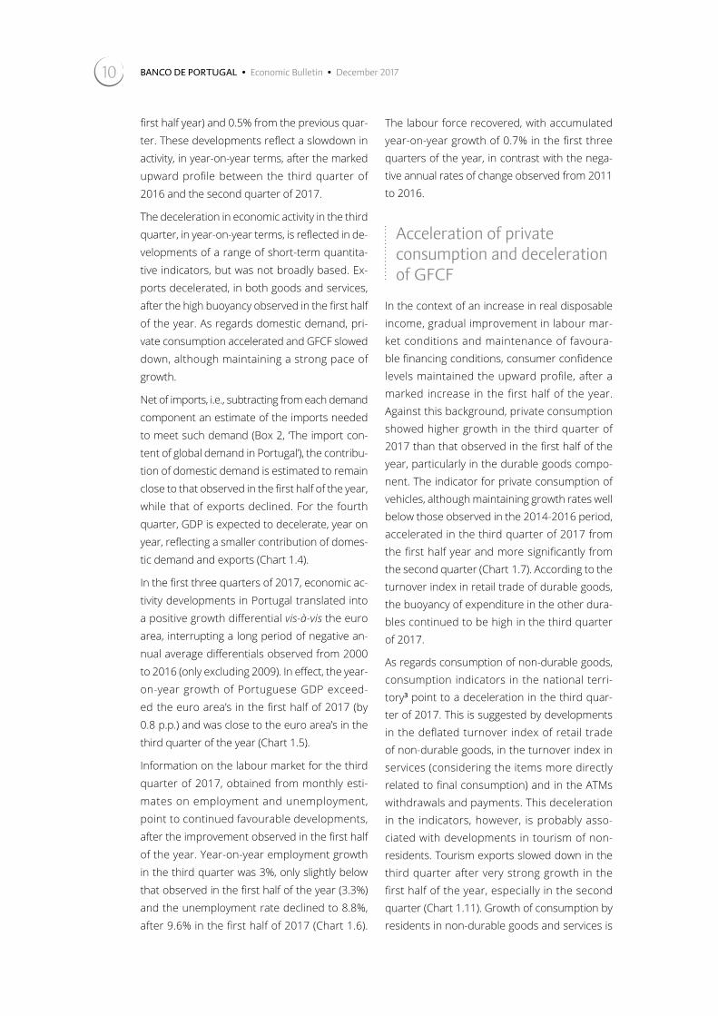
first half year) and 0.5% from the previous quar-ter. These developments reflect a slowdown in activity, in year-on-year terms, after the marked upward profile between the third quarter of 2016 and the second quarter of 2017.

The deceleration in economic activity in the third quarter, in year-on-year terms, is reflected in de-velopments of a range of short-term quantita-tive indicators, but was not broadly based. Ex-ports decelerated, in both goods and services, after the high buoyancy observed in the first half of the year. As regards domestic demand, pri-vate consumption accelerated and GFCF slowed down, although maintaining a strong pace of growth.

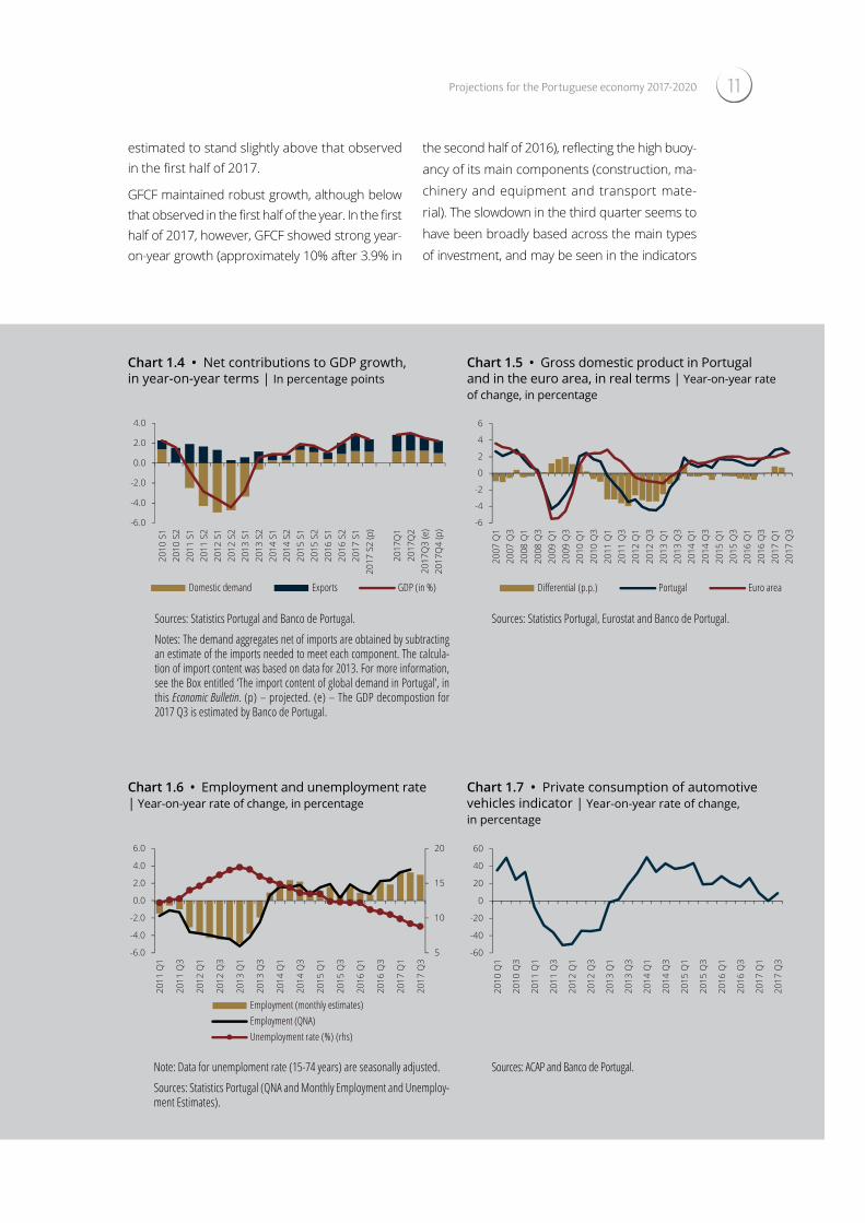
Net of imports, i.e., subtracting from each demand component an estimate of the imports needed to meet such demand (Box 2, ‘The import con-tent of global demand in Portugal’), the contribu-tion of domestic demand is estimated to remain close to that observed in the first half of the year, while that of exports declined. For the fourth quarter, GDP is expected to decelerate, year on year, reflecting a smaller contribution of domes-tic demand and exports (Chart 1.4).

In the first three quarters of 2017, economic ac-tivity developments in Portugal translated into a positive growth differential vis-à-vis the euro area, interrupting a long period of negative an-nual average differentials observed from 2000 to 2016 (only excluding 2009). In effect, the year-on-year growth of Portuguese GDP exceed-ed the euro area’s in the first half of 2017 (by 0.8 p.p.) and was close to the euro area’s in the third quarter of the year (Chart 1.5).

Information on the labour market for the third quarter of 2017, obtained from monthly esti-mates on employment and unemployment, point to continued favourable developments, after the improvement observed in the first half of the year. Year-on-year employment growth in the third quarter was 3%, only slightly below that observed in the first half of the year (3.3%) and the unemployment rate declined to 8.8%, after 9.6% in the first half of 2017 (Chart 1.6).

The labour force recovered, with accumulated year-on-year growth of 0.7% in the first three quarters of the year, in contrast with the nega-tive annual rates of change observed from 2011 to 2016.

Acceleration of private consumption and deceleration of GFCF

In the context of an increase in real disposable income, gradual improvement in labour mar-ket conditions and maintenance of favoura-ble financing conditions, consumer confidence levels maintained the upward profile, after a marked increase in the first half of the year. Against this background, private consumption showed higher growth in the third quarter of 2017 than that observed in the first half of the year, particularly in the durable goods compo-nent. The indicator for private consumption of vehicles, although maintaining growth rates well below those observed in the 2014-2016 period, accelerated in the third quarter of 2017 from the first half year and more significantly from the second quarter (Chart 1.7). According to the turnover index in retail trade of durable goods, the buoyancy of expenditure in the other dura-bles continued to be high in the third quarter of 2017.

As regards consumption of non-durable goods, consumption indicators in the national terri-tory3 point to a deceleration in the third quar-ter of 2017. This is suggested by developments in the deflated turnover index of retail trade of non-durable goods, in the turnover index in services (considering the items more directly related to final consumption) and in the ATMs withdrawals and payments. This deceleration in the indicators, however, is probably asso-ciated with developments in tourism of non-residents. Tourism exports slowed down in the third quarter after very strong growth in the first half of the year, especially in the second quarter (Chart 1.11). Growth of consumption by residents in non-durable goods and services is


Chart 1.4 • Net contributions to GDP growth, in year-on-year terms | In percentage points

Chart 1.5 • Gross domestic product in Portugal and in the euro area, in real terms | Year-on-year rate of change, in percentage

-6.0

-4.0

-2.0

0.0

2.0

4.0

2010

S1

2010

S2

2011

S1

2011

S2

2012

S1

2012

S2

2013

S1

2013

S2

2014

S1

2014

S2

2015

S1

2015

S2

2016

S1

2016

S2

2017

S1

2017

S2

(p)

2017

Q1

2017

Q2

2017

Q3

(e)

2017

Q4

(p)

Domestic demand Exports GDP (in %)

-6

-4

-2

0

2

4

6

2007

Q1

2007

Q3

2008

Q1

2008

Q3

2009

Q1

2009

Q3

2010

Q1

2010

Q3

2011

Q1

2011

Q3

2012

Q1

2012

Q3

2013

Q1

2013

Q3

2014

Q1

2014

Q3

2015

Q1

2015

Q3

2016

Q1

2016

Q3

2017

Q1

2017

Q3

Differential (p.p.) Portugal Euro area

Sources: Statistics Portugal and Banco de Portugal.

Notes: The demand aggregates net of imports are obtained by subtracting an estimate of the imports needed to meet each component. The calcula-tion of import content was based on data for 2013. For more information, see the Box entitled ‘The import content of global demand in Portugal‛, in this Economic Bulletin. (p) – projected. (e) – The GDP decompostion for 2017 Q3 is estimated by Banco de Portugal.

Sources: Statistics Portugal, Eurostat and Banco de Portugal.

Chart 1.6 • Employment and unemployment rate | Year-on-year rate of change, in percentage

Chart 1.7 • Private consumption of automotive vehicles indicator | Year-on-year rate of change, in percentage

5

10

15

20

-6.0

-4.0

-2.0

0.0

2.0

4.0

6.0

2011

Q1

2011

Q3

2012

Q1

2012

Q3

2013

Q1

2013

Q3

2014

Q1

2014

Q3

2015

Q1

2015

Q3

2016

Q1

2016

Q3

2017

Q1

2017

Q3

Employment (monthly estimates) Employment (QNA) Unemployment rate (%) (rhs)

-60

-40

-20

0

20

40

60

2010

Q1

2010

Q3

2011

Q1

2011

Q3

2012

Q1

2012

Q3

2013

Q1

2013

Q3

2014

Q1

2014

Q3

2015

Q1

2015

Q3

2016

Q1

2016

Q3

2017

Q1

2017

Q3

Note: Data for unemploment rate (15-74 years) are seasonally adjusted.

Sources: Statistics Portugal (QNA and Monthly Employment and Unemploy-ment Estimates).

Sources: ACAP and Banco de Portugal.

estimated to stand slightly above that observed in the first half of 2017.

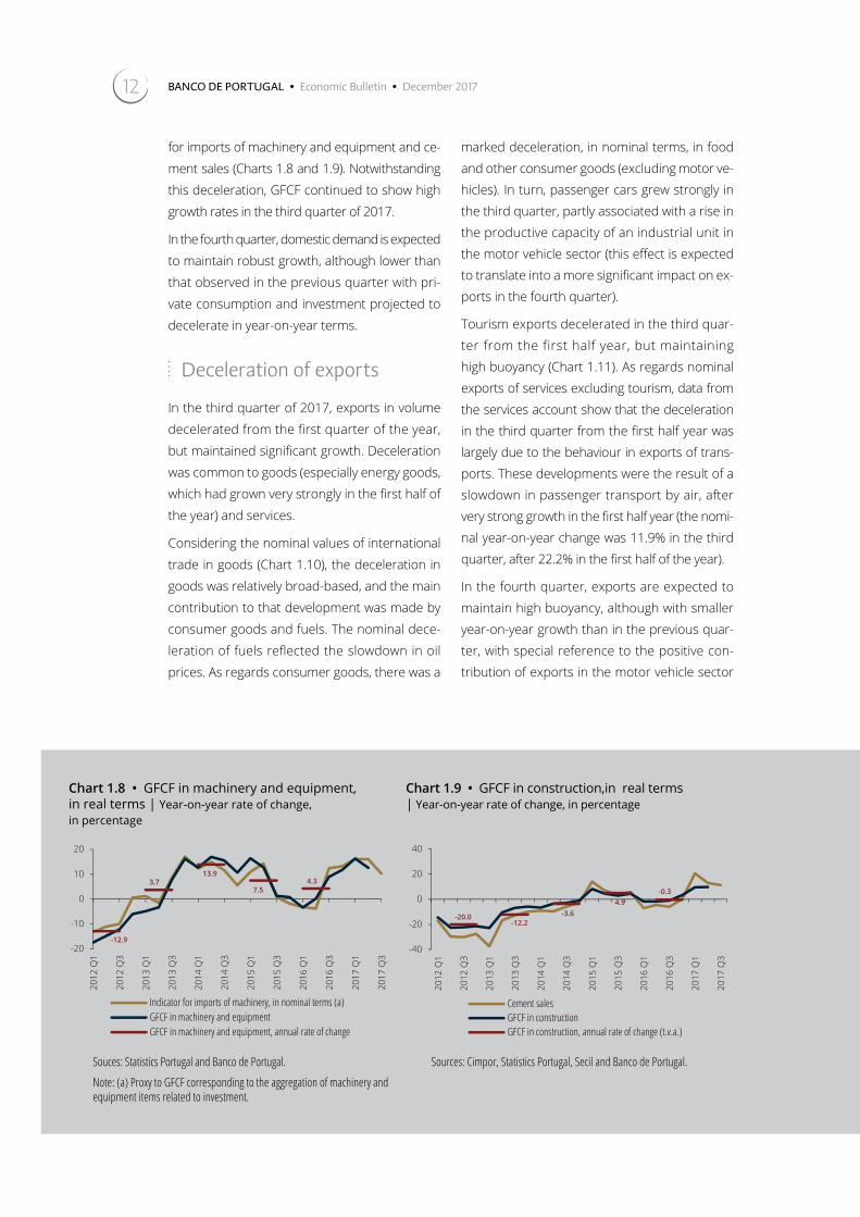
GFCF maintained robust growth, although below that observed in the first half of the year. In the first half of 2017, however, GFCF showed strong year-on-year growth (approximately 10% after 3.9% in

the second half of 2016), reflecting the high buoy-ancy of its main components (construction, ma-chinery and equipment and transport mate-rial). The slowdown in the third quarter seems to have been broadly based across the main types of investment, and may be seen in the indicators


for imports of machinery and equipment and ce-

ment sales (Charts 1.8 and 1.9). Notwithstanding

this deceleration, GFCF continued to show high

growth rates in the third quarter of 2017.

In the fourth quarter, domestic demand is expected

to maintain robust growth, although lower than

that observed in the previous quarter with pri-

vate consumption and investment projected to

decelerate in year-on-year terms.

Deceleration of exports

In the third quarter of 2017, exports in volume

decelerated from the first quarter of the year,

but maintained significant growth. Deceleration

was common to goods (especially energy goods,

which had grown very strongly in the first half of

the year) and services.

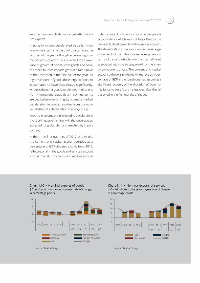
Considering the nominal values of international

trade in goods (Chart 1.10), the deceleration in

goods was relatively broad-based, and the main

contribution to that development was made by

consumer goods and fuels. The nominal dece-

leration of fuels reflected the slowdown in oil

prices. As regards consumer goods, there was a

marked deceleration, in nominal terms, in food and other consumer goods (excluding motor ve-hicles). In turn, passenger cars grew strongly in the third quarter, partly associated with a rise in the productive capacity of an industrial unit in the motor vehicle sector (this effect is expected to translate into a more significant impact on ex-ports in the fourth quarter).

Tourism exports decelerated in the third quar-ter from the first half year, but maintaining high buoyancy (Chart 1.11). As regards nominal exports of services excluding tourism, data from the services account show that the deceleration in the third quarter from the first half year was largely due to the behaviour in exports of trans-ports. These developments were the result of a slowdown in passenger transport by air, after very strong growth in the first half year (the nomi-nal year-on-year change was 11.9% in the third quarter, after 22.2% in the first half of the year).

In the fourth quarter, exports are expected to maintain high buoyancy, although with smaller year-on-year growth than in the previous quar-ter, with special reference to the positive con-tribution of exports in the motor vehicle sector

Chart 1.8 • GFCF in machinery and equipment, in real terms | Year-on-year rate of change, in percentage

Chart 1.9 • GFCF in construction,in real terms | Year-on-year rate of change, in percentage

-12.9

3.713.9

7.54.3

-20

-10

0

10

20

2012

Q1

2012

Q3

2013

Q1

2013

Q3

2014

Q1

2014

Q3

2015

Q1

2015

Q3

2016

Q1

2016

Q3

2017

Q1

2017

Q3

Indicator for imports of machinery, in nominal terms (a)GFCF in machinery and equipmentGFCF in machinery and equipment, annual rate of change

-20.0-12.2

-3.64.9

-0.3

-40

-20

0

20

40

2012

Q1

2012

Q3

2013

Q1

2013

Q3

2014

Q1

2014

Q3

2015

Q1

2015

Q3

2016

Q1

2016

Q3

2017

Q1

2017

Q3

Cement salesGFCF in constructionGFCF in construction, annual rate of change (t.v.a.)

Souces: Statistics Portugal and Banco de Portugal.

Note: (a) Proxy to GFCF corresponding to the aggregation of machinery and equipment items related to investment.

Sources: Cimpor, Statistics Portugal, Secil and Banco de Portugal.


and the continued high pace of growth of tour-ism exports.

Imports in volume decelerated also slightly on year-on-year terms in the third quarter from the first half of the year, although accelerating from the previous quarter. This reflected the slower pace of growth of non-tourism goods and servi-ces, while tourism imports grew at a rate similar to that recorded in the first half of the year. As regards imports of goods, the energy component is estimated to have decelerated significantly, whereas the other goods accelerated. Indications from international trade data in nominal terms are qualitatively similar, in spite of a more marked deceleration in goods, resulting from the addi-tional effect of a deceleration in energy prices.

Imports in volume are projected to decelerate in the fourth quarter, in line with the deceleration expected for global demand weighed by import content.

In the three first quarters of 2017 as a whole, the current and capital account surplus as a percentage of GDP declined slightly from 2016, reflecting a fall in the goods and services account surplus. The fall in the goods and services account

balance was due to an increase in the goods

account deficit which was not fully offset by the

favourable developments of the services account.

The deterioration in the goods account was large-

ly the result of the unfavourable developments in

terms of trade (particularly in the first half year)

associated with the strong growth of the ener-

gy component prices. The current and capital

account balance is projected to improve as a per-

centage of GDP in the fourth quarter, assuming a

significant recovery of the allocation of Commu-

nity funds to beneficiary institutions, after the fall

observed in the first months of the year.

Chart 1.10 • Nominal exports of goods | Contributions to the year-on-year rate of change, in percentage points

Chart 1.11 • Nominal exports of services | Contributions to the year-on-year rate of change, in percentage points

-10

0

10

20

2013 2014 2015 2016 2016 2016 2017 2017 2017

Q3 Q4 Q1 Q2 Q3

Consumption goods Intermediate goodsMachinery Transport equipmentFuels Total (%)

-5

0

5

10

15

20

2013 2014 2015 2016 2016 2016 2017 2017 2017

Q3 Q4 Q1 Q2 Q3

Travel TransportOther services Total (%)

Source: Statistics Portugal. Source: Statistics Portugal.

14 BANCO DE PORTUGAL • Economic Bulletin • December 2017

Box 1 | Projection assumptions

The projections released in this Bulletin are based on a range of assumptions for the exter-nal framework of the Portuguese economy, consistent with the Eurosystem's projection exercise published on 14 December. The main technical assumptions can be found in Table C.1.1. and the cut-off date was 28 November.

As regards the international framework, world activity is expected to accelerate in the 2017-2018 period, followed by a slight deceleration in 2019 and 2020. World trade is projected to maintain robust growth over the projection horizon, but slowing down from 2018 onwards. After the signi-ficant improvement observed in 2017, external demand for Portuguese goods and services may accelerate slightly in 2018 (to 4.9%, after 4.8% in 2017), followed by a downward profile. In com-parison to the assumptions published in previous projection exercises, both world activity and external demand were revised upwards in 2017 and 2018. The deceleration projected for 2018 onwards will be more marked in extra-EU markets, which also saw a sharper aceleration in 2017. On average, in the 2018-2020 period, external demand from intra and extra-EU markets will show similar growth rates (4.1% in the euro area and 4.3% in extra-EU markets).

Considering information implied in the futures market as at the cut-off date, in annual average terms, the oil price (in USD and in euros) will grow more than 20% in 2017 from the previous year, discontinuing the downward trend observed in the 2013-2016 period. Subsequently, the oil price in USD will increase moderately, to stand on average at USD 59 between 2018 and 2020. Compared with previous projection exercises, oil prices are revised upwards when expressed both in USD and euros, although in the latter case at a lower magnitude, due to the upward revision of the euro exchange rate.

Table C.1.1 • Projection assumptions

EB December 2017EB October

2017EB June 2017

2016 2017 2018 2019 2020 2017 2017 2018 2019

International environmentWorld GDP tva 3.0 3.5 3.7 3.6 3.5 3.5 3.3 3.6 3.5World trade tva 1.5 5.0 4.7 4.3 3.8 5.3 4.5 3.9 4.0External demand tva 2.0 4.8 4.9 4.0 3.6 4.5 4.5 3.9 4.0Oil prices in dollars vma 44.0 54.3 61.6 58.9 57.3 51.8 51.6 51.4 51.5Oil prices in euros vma 39.8 48.2 52.5 50.2 48.9 46.0 47.6 47.0 47.1

Monetary and financial conditions

Short-term interest rate (3-month EURIBOR) % -0.3 -0.3 -0.3 -0.1 0.1 -0.3 -0.3 -0.2 0.0Implicit interest rate in public debt % 3.3 3.1 3.0 3.0 3.0 3.2 3.2 3.1 3.1Effective exchange rate index tva 2.9 2.3 2.2 0.0 0.0 2.5 0.3 0.4 0.0Euro-dollar exchange rate vma 1.11 1.13 1.17 1.17 1.17 1.13 1.08 1.09 1.09

Sources: ECB, Bloomberg, Thomson Reuters and Banco de Portugal.

Notes: yoy – year-on-year rate of change, aav – annual average value. An increase in the exchange rate corresponds to an appreciation of the euro. The technical assumption for bilateral exchange rates assumes that the average levels observed in the two weeks prior to the cut-off date will remain stable over the projection horizon. The technical assumption for oil prices is based on futures markets. Developments in the three-month Euribor rate are based on expectations implied in futures contracts. The implicit interest rate on public debt is computed as the ratio of interest expenditure for the year to the simple average of the stock of debt at the end of the same year and at the end of the preceding year. Assumptions for the long-term interest rate on Portuguese public debt are based on an assumption for the implicit rate, which includes an assumption for the interest rate associated with new issuances.

Projections for the Portuguese economy 2017-2020 15

Interest rate levels have not been substantially revised from those assumed in previous exerci-

ses. Reflecting the conduct of the ECB’s accommodative monetary policy, the short-term interest

rate level will remain low and slightly negative in the 2017-2019 period, reaching a positive value

(0.1%) only at the end of the projection horizon. In turn, the long-term interest rate of Portuguese

public debt, for which the calculation methodology is based on an estimate of the implied rate

that adopts an assumption for the interest rate of new issues, indicates a slight and gradual decli-

ne over the projection period, to stand at 3% at the end of the period.

The technical assumption for exchange rates assumes that the average levels seen in the two

weeks prior to the cut-off date will remain stable over the projection horizon, which is reflected

in higher appreciation of the foreign exchange rate in 2018 than that implied in previous projec-

tions. In annual average terms, a similar appreciation is assumed for 2017 and 2018 (2.3% and

2.2% respectively). The euro exchange rate against the USD is also above that implied in the pro-

jection of the June issue of the Economic Bulletin, reflecting recent developments.

In line with Eurosystem rules, the projections for public finance variables include the policy mea-

sures that have already been approved (or are highly likely to be approved) and that have been

specified with sufficient detail in official fiscal documents. Therefore, among the measures inclu-

ded in the State Budget for 2018, special reference should be made to the incorporation of the

effect of the gradual unfreezing of salary progressions in the general government, the change in

in the personal income tax brackets, and the extraordinary update of pensions in August 2018. In

addition, the measures previously announced were taken into account, including the elimination

of the surcharge on the personal income tax, the update of lower pensions in August 2017, the

introduction of social inclusion benefits, and relaxed penalties for early retirement in the case of

workers with long contributory careers.

The current estimate for real growth of public consumption in 2017 stands at 0.1 per cent.

Underlying these developments is the assumption of an increase in the number of public emplo-

yees which is only partly offset by the effect of a reduction in the number of hours worked in

the general government from 40 to 35 in mid-2016. As regards expenditure in the acquisition of

goods and services, it is projected to decline slightly, in real terms, in part due to the decrease in

expenditure associated with public-private partnerships in the road sector in 2017. In 2018, the

rate of change of public consumption will no longer be affected by the effect of the decline in

working hours. On the other hand, lower savings are projected from public-private partnerships in

the road sector (in line with the State Budget for 2018). Therefore, in 2018, public consumption in

real terms is expected to accelerate. In coming years, in a context of gradual convergence towards

the stabilisation of the number of public employees, real public consumption is projected to dece-

lerate gradually.

A positive change is expected for the public consumption deflator over the projection horizon. In

2017 these developments derive from the remaining impact of the reversal of wage cuts previou-

sly in force in the general government and, from 2018 onwards, they will be due to the above-

-mentioned effect of the gradual unfreezing of salary progressions. In the last two years of the

projection horizon, wages in the general government are updated in line with price development

expectations.

As regards public investment, after the strong fall in 2016, it is expected to recover in 2017 and

2018, although less markedly than projected in the State Budget for 2018. In the other years of

the projection horizon, public investment is forecast to evolve in line with nominal GDP.


1.3. Demand, supply and external accountsThe current cycle of expansion of the Portu-guese economy will extend into the projection horizon, with activity growth rates exceeding the average available estimates for potential GDP growth. According to current projections, GDP is expected to increase by 2.6% in 2017, decelerat-ing gradually to 2.3% in 2018, 1.9% in 2019, and 1.7% in 2020. This pace of growth implies that GDP will resume by mid-2018 its level prior to the international financial crisis, to stand around 4% above that level in 2020.

As regards developments in the supply side of the economy, the recovery has been broadly-based across the main sectors of activity. In construc-tion, the Gross Value Added (GVA) only started to recover at the end of 2016, after the previous declines, while in agriculture the GVA has shown a very volatile behaviour. Reference should be made to the contribution to the ongoing recovery made by the components of services more directly related to tourism (Chart 1.12). In the first half of 2017, construction and industry were the sec-tors with the highest GVA growth, but most sec-tors had higher year-on-year rates of change than in the second half of 2016, with the inter-sectoral dispersion levels of GVA growth standing at very low levels. Over the projection horizon, GVA in

industry and construction is expected to slow down, in line with developments projected for investment and exports, while services are pro-jected to maintain relatively stable growth.

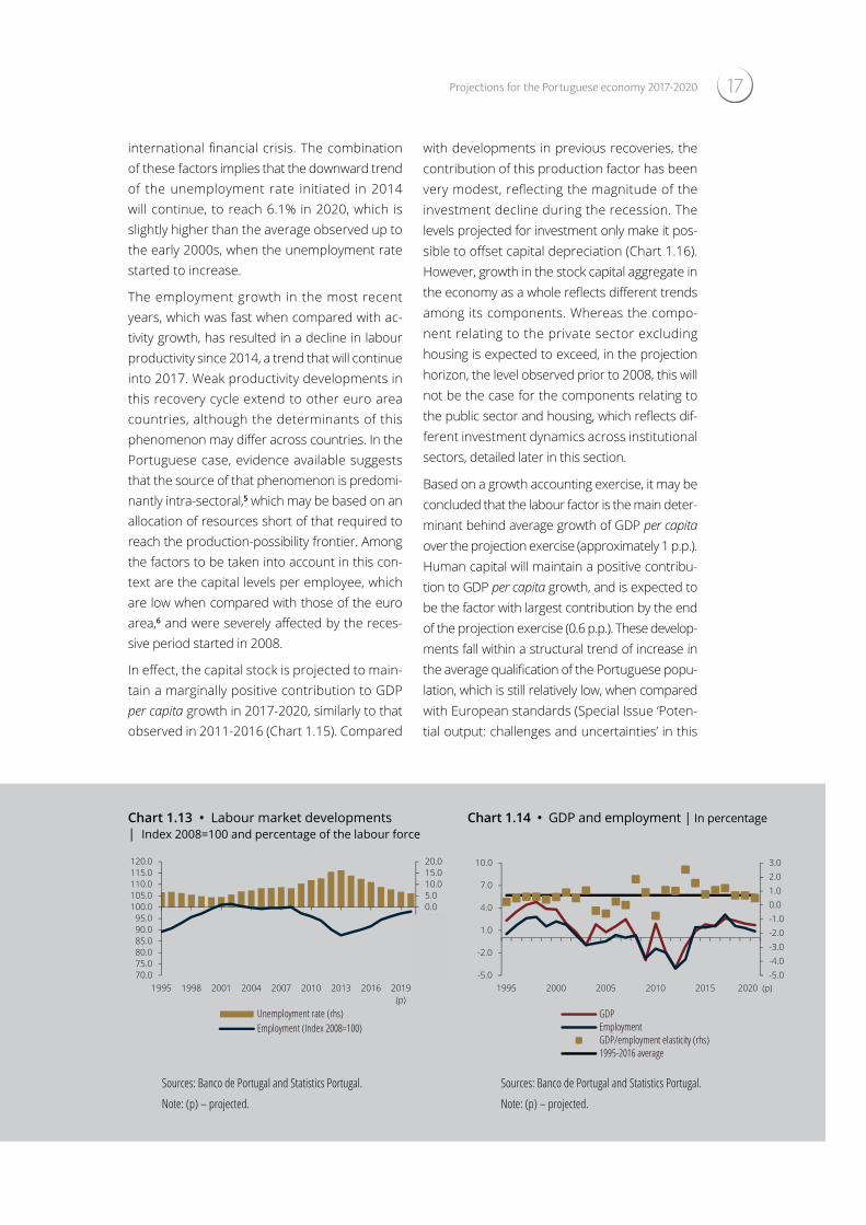
The labour market is expected to carry on the recovery trend seen in recent years (Chart 1.13). Following very expressive growth in excess of GDP’s in 2017 (3.1%), employment is expected to show a growth trend slightly below that of activity, more in line with the historical relation-ship between those two variables in recovery stages (Chart 1.14). Employment gains derive essentially from developments in private em-ployment. Public employment is also expected to recover, albeit more moderately. At the end of the projection horizon, the employment level is projected to stand at levels approximately 2% below those observed prior to the international financial crisis. Slightly positive rates of change are projected for the labour force during the projection horizon, considering that the cycli-cal recovery of the economy will lead some in-active individuals, such as discouraged work-ers, back to the labour market,4 a trend already observed in recent years. However, the main-tenance of the recent population dynamics, characterised by negative natural and migrato-ry balances, may not allow the active popula-tion to resume the levels observed prior to the

Chart 1.12 • GVA Breakdown

| Cumulative contributions to

the GVA rate of change, in

percentage points-2

0

2

4

6

8

10

12

2013 2014 2015 2016 2017 H1 2017 (p) 2018 (p) 2019 (p) 2020 (p)

Industry (including electricity, gas and water supply) Transportation and communicationFinancial and real estate activitiesGVA

Agriculture, forestry and fishingConstructionTrade, repair, accommodation and food service activities Other servicesGVA-projection


Note: (p) – projected. The dots indicate GVA projections.


international financial crisis. The combination of these factors implies that the downward trend of the unemployment rate initiated in 2014 will continue, to reach 6.1% in 2020, which is slightly higher than the average observed up to the early 2000s, when the unemployment rate started to increase.

The employment growth in the most recent years, which was fast when compared with ac-tivity growth, has resulted in a decline in labour productivity since 2014, a trend that will continue into 2017. Weak productivity developments in this recovery cycle extend to other euro area countries, although the determinants of this phenomenon may differ across countries. In the Portuguese case, evidence available suggests that the source of that phenomenon is predomi-nantly intra-sectoral,5 which may be based on an allocation of resources short of that required to reach the production-possibility frontier. Among the factors to be taken into account in this con-text are the capital levels per employee, which are low when compared with those of the euro area,6 and were severely affected by the reces-sive period started in 2008.

In effect, the capital stock is projected to main-tain a marginally positive contribution to GDP per capita growth in 2017-2020, similarly to that observed in 2011-2016 (Chart 1.15). Compared

with developments in previous recoveries, the contribution of this production factor has been very modest, reflecting the magnitude of the investment decline during the recession. The levels projected for investment only make it pos-sible to offset capital depreciation (Chart 1.16). However, growth in the stock capital aggregate in the economy as a whole reflects different trends among its components. Whereas the compo-nent relating to the private sector excluding housing is expected to exceed, in the projection horizon, the level observed prior to 2008, this will not be the case for the components relating to the public sector and housing, which reflects dif-ferent investment dynamics across institutional sectors, detailed later in this section.

Based on a growth accounting exercise, it may be concluded that the labour factor is the main deter-minant behind average growth of GDP per capita over the projection exercise (approximately 1 p.p.). Human capital will maintain a positive contribu-tion to GDP per capita growth, and is expected to be the factor with largest contribution by the end of the projection exercise (0.6 p.p.). These develop-ments fall within a structural trend of increase in the average qualification of the Portuguese popu-lation, which is still relatively low, when compared with European standards (Special Issue ‘Poten-tial output: challenges and uncertainties’ in this

Chart 1.13 • Labour market developments | Index 2008=100 and percentage of the labour force

Chart 1.14 • GDP and employment | In percentage

-30.0-25.0-20.0-15.0-10.0-5.00.05.010.015.020.0

70.075.080.085.090.095.0100.0105.0110.0115.0120.0

1995 1998 2001 2004 2007 2010 2013 2016 2019(p)

Unemployment rate (rhs)Employment (Index 2008=100)

-5.0-4.0-3.0-2.0-1.00.01.02.03.0

-5.0

-2.0

1.0

4.0

7.0

10.0

1995 2000 2005 2010 2015 2020 (p)

GDPEmploymentGDP/employment elasticity (rhs)1995-2016 average






Bulletin). Finally, total factor productivity, obtained as a residual in this exercise, points to a marginally positive contribution during the projection exer-cise, after a negative average change since the start of the euro area. This should be the result of better allocation of resources in the economy, fol-lowing a process of reorientation towards sectors more exposed to international competition.

Rebalancing of domestic demand, with more buoyant investment

Chart 1.17 illustrates the shift in expenditure seen over the past few years taking into account aggregates net of average import content, com-puted with reference to the year 2013. Since 2010 the share of domestic demand in GDP has decreased, particularly in the case of invest-ment. This downward trend in the GFCF share, which started in the beginning of the decade, was reversed in 2014, but the fall during the crisis was strong enough to impact on the supply-side of the economy as of today. The share of pri-vate and public consumption in GDP has also fol-lowed a downward path in recent years, reflecting the need for fiscal adjustment and the house-hold deleveraging process. In turn, the share of exports in GDP has increased markedly, with this buoyancy extending to the various compo-nents of exports of goods and services, most notably tourism. Overall, these trends should per-sist over the projection horizon, which points to a pattern of more sustainable growth for the Portuguese economy in the medium run.

These developments result in a relatively stable contribution of domestic demand net of import content to GDP over the projection horizon, with similar average contributions of investment and private consumption. The contribution of exports will decrease slightly, to a level below that of domestic demand in the 2018-20 period (Chart 1.18).

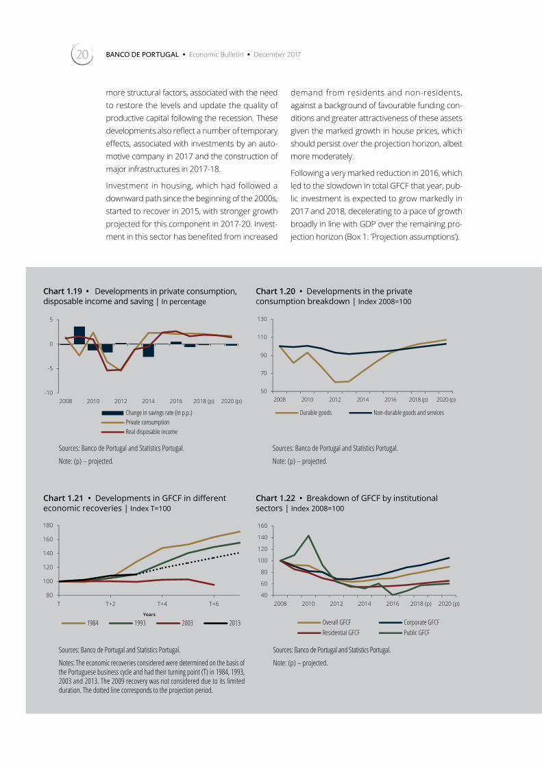
Private consumption is expected to continue to grow by approximately 2.1% in 2017-18, slow-ing down to around 1.8% in 2019-20 and, as such, slightly below GDP rates of change during most of the projection period. At the end of the

horizon projection, the share of private con-sumption in GDP should stand close to the lev-els seen prior to the financial crisis (Chart 1.17). On average over the projection horizon, pri-vate consumption growth should be broadly in line with that expected for real disposable income, indicating an overall stable savings rate (Chart 1.19).

The projected profile includes a shift in private consumption, with a slowdown in consumption of durable goods associated with the unwinding of the pent-up demand effect that followed the recession period. However, rates of change in this consumption component should remain above those of non-durable consumption, which, according to projections, will grow at a relatively stable pace over the projection horizon. Under-lying such developments is a slight acceleration in real disposable income in 2018, followed by a slowdown. Against a background of employ-ment slowdown and moderate real wage growth, developments in this aggregate are favoured in 2018-19 by the public finance variables assump-tions taken into account. Consumption should also benefit from the maintenance of favourable funding conditions, although a slight deteriora-tion is expected at the end of the horizon, which will have a mild negative impact on disposable income (Box 3: ’Effect of the interest rate increase on household income: heterogeneity by age groups and income quartiles‛). At the end of the projection horizon, the durable and non-durable components of consumption are expected to stand slightly above the levels seen prior to the international financial crisis (Chart 1.20).

Following a very substantial acceleration in 2017, to 8.3%, GFCF should continue to grow at a marked – albeit gradually more subdued – pace over the projection horizon, with a rate of change of approximately 6% in 2018-19 and 5.4% in 2020. This path means that, following slightly more dynamic developments than in previous cycles up to 2016, cumulative growth in GFCF will remain clearly above that seen in the recovery that started in 2003 (Chart 1.21). However, the fall in GFCF since the international financial crisis was unprecedented and resulted in a very substantial reduction in the share of this component in GDP,


only partly reversed at the end of the projection horizon. Notwithstanding, GFCF performed dif-ferently across institutional sectors (Chart 1.22).

The more buoyant GFCF compared with the recov-ery that started in 2003 reflects developments in corporate GFCF and, as of 2016, also residen-tial GFCF. At the end of the projection horizon,

corporate GFCF is expected to be approximately 5% higher than prior to the international financial crisis. Corporate investment developments ben-efit from a favourable macroeconomic environ-ment, particularly as regards funding conditions, the maintenance of an expected growth outlook for demand, amid low uncertainty, as well as from

Chart 1.15 • Breakdown of the growth in real GDP per capita | Contributions in percentage points

Chart 1.16 • Developments in the contribution of the capital stock per capita in different economic recoveries | Index T=100

-2.5-2.0-1.5-1.0-0.50.00.51.01.52.02.5

1999-2010 2011-2016 2017-2020 (p)

Employment per capita Human capital

Capital stock per capita Total factor productivity GDP per capita (arc, in %)

98

103

108

113

T T+2 T+4 T+6Years

1984 1993 2003 2013

Sources: Barro and Lee (2013), Banco de Portugal, Quadros de Pessoal and Statistics Portugal.

Notes: (p) – projected. The growth accounting exercise of GDP per capita is based on a Cobb-Douglas production function. The measures of human ca-pital were constructed from the data of Barro and Lee (2013) ’A new data set of educational attainment in the world, 1950-2010′, Journal of Development Economics 104, pp. 184-198. For Portugal, these series were annualized and extended using the profile of the average years of education of employment of Quadros de Pessoal (until 2012), the Labour Force Survey of INE (from 2013 to 2015) and the projections available in http://www.barrolee.com/.



Chart 1.17 • Developments in GDP breakdown | In percentage

Chart 1.18 • Net contributions to GDP growth | In percentage points

0

10

20

30

40

50

60

0

5

10

15

20

25

30

35

1995 2000 2005 2010 2015 2020(p)

Public consumption InvestmentExports Private Consumption (rhs)

0.0

1.0

2.0

3.0

2014 2015 2016 2017 (p) 2018 (p) 2019 (p) 2020 (p)

Domestic Demand Exports


Notes: (p) – projected. The expenditure components considered are net of imports, i.e., adjusted by the respective average import content.


Notes: (p) – projected. The expenditure components considered are net of imports, i.e., adjusted by the respective average import content.


more structural factors, associated with the need to restore the levels and update the quality of productive capital following the recession. These developments also reflect a number of temporary effects, associated with investments by an auto-motive company in 2017 and the construction of major infrastructures in 2017-18.

Investment in housing, which had followed a downward path since the beginning of the 2000s, started to recover in 2015, with stronger growth projected for this component in 2017-20. Invest-ment in this sector has benefited from increased

demand from residents and non-residents, against a background of favourable funding con-ditions and greater attractiveness of these assets given the marked growth in house prices, which should persist over the projection horizon, albeit more moderately.

Following a very marked reduction in 2016, which led to the slowdown in total GFCF that year, pub-lic investment is expected to grow markedly in 2017 and 2018, decelerating to a pace of growth broadly in line with GDP over the remaining pro-jection horizon (Box 1: ’Projection assumptions‛).

Chart 1.19 • Developments in private consumption, disposable income and saving | In percentage

Chart 1.20 • Developments in the private consumption breakdown | Index 2008=100

-10

-5

0

5

2008 2010 2012 2014 2016 2018 (p) 2020 (p)

Change in savings rate (in p.p.) Private consumptionReal disposable income

50

70

90

110

130

2008 2010 2012 2014 2016 2018 (p) 2020 (p)

Durable goods Non-durable goods and services





Chart 1.21 • Developments in GFCF in different economic recoveries | Index T=100

Chart 1.22 • Breakdown of GFCF by institutional sectors | Index 2008=100

80

100

120

140

160

180

T T+2 T+4 T+6

Years

1984 1993 2003 2013

40

60

80

100

120

140

160

2008 2010 2012 2014 2016 2018 (p) 2020 (p)

Overall GFCFResidential GFCF

Corporate GFCF Public GFCF






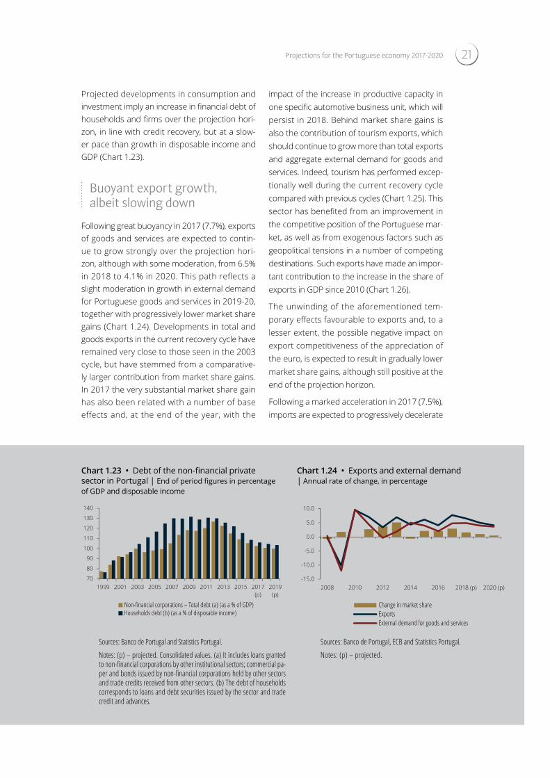
Projected developments in consumption and investment imply an increase in financial debt of households and firms over the projection hori-zon, in line with credit recovery, but at a slow-er pace than growth in disposable income and GDP (Chart 1.23).

Buoyant export growth, albeit slowing down

Following great buoyancy in 2017 (7.7%), exports of goods and services are expected to contin-ue to grow strongly over the projection hori-zon, although with some moderation, from 6.5% in 2018 to 4.1% in 2020. This path reflects a slight moderation in growth in external demand for Portuguese goods and services in 2019-20, together with progressively lower market share gains (Chart 1.24). Developments in total and goods exports in the current recovery cycle have remained very close to those seen in the 2003 cycle, but have stemmed from a comparative-ly larger contribution from market share gains. In 2017 the very substantial market share gain has also been related with a number of base effects and, at the end of the year, with the

impact of the increase in productive capacity in one specific automotive business unit, which will persist in 2018. Behind market share gains is also the contribution of tourism exports, which should continue to grow more than total exports and aggregate external demand for goods and services. Indeed, tourism has performed excep-tionally well during the current recovery cycle compared with previous cycles (Chart 1.25). This sector has benefited from an improvement in the competitive position of the Portuguese mar-ket, as well as from exogenous factors such as geopolitical tensions in a number of competing destinations. Such exports have made an impor-tant contribution to the increase in the share of exports in GDP since 2010 (Chart 1.26).

The unwinding of the aforementioned tem-porary effects favourable to exports and, to a lesser extent, the possible negative impact on export competitiveness of the appreciation of the euro, is expected to result in gradually lower market share gains, although still positive at the end of the projection horizon.

Following a marked acceleration in 2017 (7.5%), imports are expected to progressively decelerate

Chart 1.23 • Debt of the non-financial private sector in Portugal | End of period figures in percentage of GDP and disposable income

Chart 1.24 • Exports and external demand | Annual rate of change, in percentage

70

80

90

100

110

120

130

140

1999 2001 2003 2005 2007 2009 2011 2013 2015 2017(p)

2019(p)

Non-financial corporations – Total debt (a) (as a % of GDP)Households debt (b) (as a % of disposable income)

-15.0

-10.0

-5.0

0.0

5.0

10.0

2008 2010 2012 2014 2016 2018 (p) 2020 (p)

Change in market shareExportsExternal demand for goods and services


Notes: (p) – projected. Consolidated values. (a) It includes loans granted to non-financial corporations by other institutional sectors; commercial pa-per and bonds issued by non-financial corporations held by other sectors and trade credits received from other sectors. (b) The debt of households corresponds to loans and debt securities issued by the sector and trade credit and advances.

Sources: Banco de Portugal, ECB and Statistics Portugal.

Notes: (p) – projected.


throughout the 2018-20 period, reaching 4.8% growth at the end of the projection horizon. The projected dynamics extend to goods and ser-vices components and point to developments broadly in line with the average import-con-tent-weighted global demand elasticity seen in the past. This leads to a greater penetration of imports over the projection horizon (Chart 1.27). The slowdown in imports in 2018-20 – taking into account the average import content of the

expenditure components, i.e. the counterpart of Chart 1.18 – chiefly results from the projected profile for exports and, to a lesser extent, from the shift in private consumption towards lower growth in the durable goods component, which has greater import content (Chart 1.28).

Strengthening of the economy’s net lending position

Chart 1.25 • Developments in tourism exports in different economic recoveries | Index T=100

Chart 1.26 • Weight of exports on GDP | In percentage

80

100

120

140

160

180

200

220

T T+2 T+4 T+6Years

1984 1993 2003 2013

0

20

40

60

1995 2000 2005 2010 2015 2020 (p)

Overall exports TourismServices excluding tourism Goods


Notes: The economic recoveries considered were determined on the basis of the Portuguese business cycle and had their turning point (T) in 1984, 1993, 2003 and 2013. The 2009 recovery was not considered due to its limited du-ration. The dotted line corresponds to the projection period.



Chart 1.27 • Imports and import-content weighted global demand | In percentage

Chart 1.28 • Breakdown of imports by global demand components | Contributions in percentage points

-10.0

-5.0

0.0

5.0

10.0

2008 2010 2012 2014 2016 2018 (p) 2020 (p)

Import penetration Weighted global demandImports

-10.0

-5.0

0.0

5.0

10.0

2011 2014 2017(p)

2020(p)

Private consumption Public consumptionGFCF Change in inventoriesExports Imports






The Portuguese economy is expected to main-

tain a net lending position over the projection

horizon, similarly to that seen since 2012. Fol-

lowing a slight reduction in the current and capi-

tal account balance as a percentage of GDP in

2017 (1.5%), net lending is expected to increase

in 2018, remaining at around 2.2% of GDP up

to 2020.

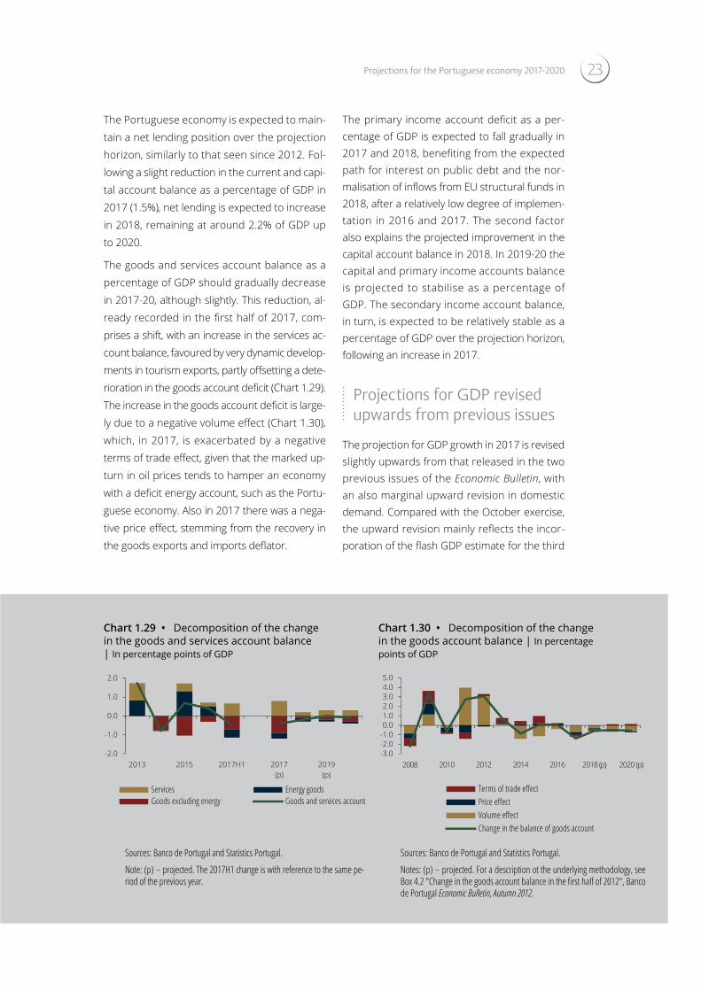
The goods and services account balance as a

percentage of GDP should gradually decrease

in 2017-20, although slightly. This reduction, al-

ready recorded in the first half of 2017, com-

prises a shift, with an increase in the services ac-

count balance, favoured by very dynamic develop-

ments in tourism exports, partly offsetting a dete-

rioration in the goods account deficit (Chart 1.29).

The increase in the goods account deficit is large-

ly due to a negative volume effect (Chart 1.30),

which, in 2017, is exacerbated by a negative

terms of trade effect, given that the marked up-

turn in oil prices tends to hamper an economy

with a deficit energy account, such as the Portu-

guese economy. Also in 2017 there was a nega-

tive price effect, stemming from the recovery in

the goods exports and imports deflator.

The primary income account deficit as a per-centage of GDP is expected to fall gradually in 2017 and 2018, benefiting from the expected path for interest on public debt and the nor-malisation of inflows from EU structural funds in 2018, after a relatively low degree of implemen-tation in 2016 and 2017. The second factor also explains the projected improvement in the capital account balance in 2018. In 2019-20 the capital and primary income accounts balance is projected to stabilise as a percentage of GDP. The secondary income account balance, in turn, is expected to be relatively stable as a percentage of GDP over the projection horizon, following an increase in 2017.

Projections for GDP revised upwards from previous issues

The projection for GDP growth in 2017 is revised slightly upwards from that released in the two previous issues of the Economic Bulletin, with an also marginal upward revision in domestic demand. Compared with the October exercise, the upward revision mainly reflects the incor-poration of the flash GDP estimate for the third

Chart 1.29 • Decomposition of the change in the goods and services account balance | In percentage points of GDP

Chart 1.30 • Decomposition of the change in the goods account balance | In percentage points of GDP

-2.0

-1.0

0.0

1.0

2.0

2013 2015 2017H1 2017(p)

2019(p)

Services Energy goodsGoods excluding energy Goods and services account

-3.0-2.0-1.00.01.02.03.04.05.0

2008 2010 2012 2014 2016 2018 (p) 2020 (p)

Terms of trade effectPrice effectVolume effectChange in the balance of goods account


Note: (p) – projected. The 2017H1 change is with reference to the same pe-riod of the previous year.


Notes: (p) – projected. For a description ot the underlying methodology, see Box 4.2 "Change in the goods account balance in the first half of 2012", Banco de Portugal Economic Bulletin, Autumn 2012.


quarter of 2017 and recent conjunctural data, with more favourable than expected develop-ments. Compared with the June Economic Bul-letin, projections of more subdued growth in exports and imports result from the incorpo-ration of National Accounts information for the first half of the year. Such revisions produce dynamic effects with an impact that extends into the following year, which, however, are offset by stronger domestic demand growth in 2018 and 2019. This growth reflects updated public finance assumptions (Box 1: ’Projection assump-tions‛) as well as, in 2018, the positive effects stemming from the incorporation of more recent conjunctural information. This rebalancing in global demand implies an upward revision of GDP growth projected for 2018 and 2019 from the June Economic Bulletin.

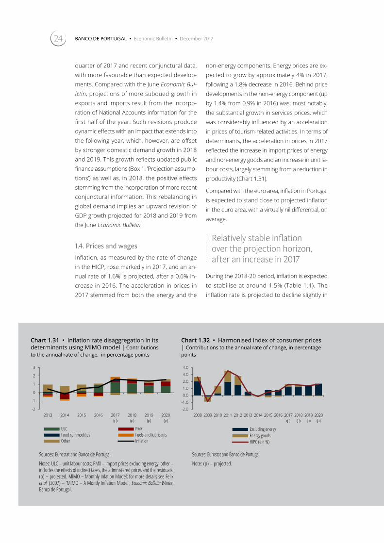
1.4. Prices and wagesInflation, as measured by the rate of change in the HICP, rose markedly in 2017, and an an-nual rate of 1.6% is projected, after a 0.6% in-crease in 2016. The acceleration in prices in 2017 stemmed from both the energy and the

non-energy components. Energy prices are ex-pected to grow by approximately 4% in 2017, following a 1.8% decrease in 2016. Behind price developments in the non-energy component (up by 1.4% from 0.9% in 2016) was, most notably, the substantial growth in services prices, which was considerably influenced by an acceleration in prices of tourism-related activities. In terms of determinants, the acceleration in prices in 2017 reflected the increase in import prices of energy and non-energy goods and an increase in unit la-bour costs, largely stemming from a reduction in productivity (Chart 1.31).

Compared with the euro area, inflation in Portugal is expected to stand close to projected inflation in the euro area, with a virtually nil differential, on average.

Relatively stable inflation over the projection horizon, after an increase in 2017

During the 2018-20 period, inflation is expected to stabilise at around 1.5% (Table 1.1). The inflation rate is projected to decline slightly in

Chart 1.31 • Inflation rate disaggregation in its determinants using MIMO model | Contributions to the annual rate of change, in percentage points

Chart 1.32 • Harmonised index of consumer prices | Contributions to the annual rate of change, in percentage points

-2

-1

0

1

2

3

2013 2014 2015 2016 2017(p)

2018(p)

2019(p)

2020(p)

ULC PMXFood commodities Fuels and lubricantsOther Inflation

-2.0

-1.0

0.0

1.0

2.0

3.0

4.0

2008 2009 2010 2011 2012 2013 2014 2015 2016 2017 (p)

2018 (p)

2019 (p)

2020 (p)

Excluding energyEnergy goodsHIPC (em %)

Sources: Eurostat and Banco de Portugal.

Notes: ULC – unit labour costs; PMX – import prices excluding energy; other – includes the effects of indirect taxes, the admnistered prices and the residuals. (p) – projected. MIMO – Monthly Infation Model: for more details see Felix et al. (2007) – ’MIMO – A Montly Inflation Model‛, Economic Bulletin Winter, Banco de Portugal.

Sources: Eurostat and Banco de Portugal.



2018, influenced by developments in the energy component, with a subdued price increase be-low that seen in 2017. In 2019 and 2020, con-tributions of energy prices to inflation should be virtually nil, in line with the assumptions for oil prices. Non-energy prices are expected to make a positive and increasingly greater con-tribution in the 2018-20 period (Chart 1.32), chiefly reflecting the acceleration in non-energy industrial goods prices, after falls in prices since 2012. Compared with the June and October is-sues of the Economic Bulletin, inflation levels for the 2017-19 period have remained virtually un-changed.

Underlying the slightly upward developments expected for inflation excluding energy goods in the 2017-20 period is a favourable domes-tic and external environment, with the protrac-tion of an upturn in activity, the continued im-pact of monetary policy measures implemented by the ECB, and the maintenance of favourable financing conditions. At domestic level, nominal wages per employee are expected to grow mod-erately, against an improvement in labour mar-ket conditions, via an increase in employment

and the maintenance of the downward profile in the unemployment rate and a slight rise in pro-ductivity (Chart 1.33).

Import prices have accelerated markedly in 2017, reflecting a strong increase in oil and other com-modity prices. Developments in the export defla-tor were similar, but growth was more muted (given the greater share of oil products in the case of imports), which led to a decrease in terms of trade in 2017. During the 2018-20 period, these deflators are expected to grow at a moder-ate and relatively stable pace, amid a lack of pressure from the energy component. Export prices should grow slightly more than those in imports, which would result in a slight improve-ment in terms of trade.

The GDP deflator is expected to follow a slightly upward path between 2017 and 2020. Unit labour costs should decelerate in 2018 – chiefly due to the recovery in productivity growth – and subsequently maintain relatively stable growth, reflecting the combined effect of an acceleration in nominal wages and greater productivity growth. Gross operational surplus per unit of output is expected to increase moderately between 2018

Chart 1.33 • HICP excluding energy | Annual rate of change, in percentage

Chart 1.34 • Inflation forecasts for Portugal and the euro area | Annual rate of change, in percentage

-3-2-1012345

2010 2011 2012 2013 2014 2015 2016 2017(p)

2018(p)

2019(p)

2020(p)

Compensation per employeeImport prices excluding energyHIPC excluding energy

-0.50

0.00

0.50

1.00

1.50

2.00

Jan.

201

3

Jul.

2013

Jan.

201

4

Jul.

2014

Jan.

201

5

Jul.

2015

Jan.

201

6

Jul.

2016

Jan.

201

7

Jul.

2017

Next 12 months forecast for PortugalNext 12 months forecast for euro area



Source: Consensus Economics.


and 2020 after a decline in 2017, partly reflecting adverse developments in terms of trade.

Higher inflation expectations in 2017

Inflation expectations for the next 12 months, calculated on the basis of Consensus Economics data, point to an increase in 2017 in Portugal and the euro area. Available information indicates that inflation expected in the first half of 2017 has followed an upward path, decelerating some-what in recent months (up to November). In 2017 and compared with the previous year, projected figures were closer, although still below, the ECB’s price stability objective of a rate of change in HICP close to, but below, 2% in the medium term (Chart 1.34). Additionally, inflation expectations for Portugal and for the euro area have converged in recent months.

1.5. Uncertainty and risks

Downside risks to activity and upside risks to inflation in the medium run

Over the projection horizon, a number of risk fac-tors may affect the most likely scenario reflected in the current projections. Risks to activity are mostly external. Downside risks to activity include a possible deterioration in geopolitical tensions at international level, most notably developments in Catalonia (Box 4: ’Macroeconomic impact of the crisis in Catalonia‛). The possibility that advanced economies may adopt protectionist measures in the medium run, including the possibility of a more adverse impact of the UK’s exit from the EU, may also add to global political uncertainty. Finally, a more substantial economic adjustment in a number of highly indebted emerging mar-ket economies, particularly China, cannot be ruled out. In addition to the negative downside impact on external demand for Portuguese goods and services, these risks may also have repercussions on the confidence of economic

agents, commodity prices and on a possible further appreciation of the euro. The possibility of an upsurge in financial market tensions may make the monetary and financial environment less favourable than anticipated, with an impact on developments in consumption and invest-ment, taking into account the possible increase in funding costs. In the euro area, the persis-tence of vulnerabilities in the banking system of some countries may amplify this risk.

However, these risks may be mitigated by the possibility that the current cyclical moment will turn out to be stronger than anticipated at global and domestic level, taking into account the con-tinued improvement in economic agents’ confi-dence and the potential impact of the announced US fiscal policy measures. Moreover, at domestic level, it must also be considered that the recent house price dynamics may have a greater-than-expected impact on investment in this sector and on private consumption.

Turning to inflation, upside risk factors are associ-ated with possible further increases in the mini-mum wage in 2018 and 2019 and, to a lesser extent, with the aforementioned possibility of a more protectionist trade policy. These risks are partially offset by the possibility that non-energy industrial goods prices maintain the downward path seen since 2012.

As a result of this analysis, there is a low probabil-ity that external demand will post more adverse developments than those considered in the most likely scenario in 2018-19 (for 2017, the afore-mentioned risk factors are considered to cancel out) (Table 1.2). The possibilities of an apprecia-tion of the euro and marginally higher long-term interest rates in 2018-19 were also taken into account.

At domestic level, a probability of 55% was con-sidered that private consumption and invest-ment may grow above projections for 2017, due to more marked cyclical dynamics. In the medium term, however, this effect is more than compensated by downside factors that may affect consumer and entrepreneurs’ con-fidence. As such, there is a marginal probability


Chart 1.35 • Gross domestic product | Rate of change, in percentage

Chart 1.36 • Harmonized index of consumer prices | Rate of change, in percentage

-1.0

0.0

1.0

2.0

3.0

4.0

5.0

2014 2015 2016 2017 2018 2019-2.0

-1.0

0.0

1.0

2.0

3.0

4.0

5.0

2014 2015 2016 2017 2018 2019

Sources: Banco de Portugal and Statistics Portugal. Sources: Banco de Portugal and Statistics Portugal.

that these aggregates show more muted de-velopments in 2018-19. Furthermore, a proba-bility of 55% was considered that real wages grow more than projected for 2018-19, as well as a marginal probability that inflation is above projections for 2018-19.

This analysis points to slightly upside risks to activity in 2017 and downside risks in 2018-19. Upside risks to nominal wages result in a mar-ginally upside risk to inflation in 2018-19.

Table 1.2 • Risk factors – Probability of an outcome below the implicit in the projections | In percentage

2017 2018 2019

Projection assumptionsLong-term interest rate 50 51 51Exchange rate 50 46 44External demand 50 53 51

Endogenous variablesPrivate consumption 45 51 52GFCF 45 53 53Wages 50 45 45HICP 50 49 49

Source: Banco de Portugal.

Table 1.3 • Probability of an outcome below the projections | In percentage

Weights 2017 2018 2019

Gross domestic product 100 47 54 55Private consumption 66 40 51 54GFCF 15 43 54 55Exports 40 50 53 53Imports 39 45 53 55

HICP 51 47 45


2012 ‐3,3 ‐3,3 ‐3,3 ‐3,3 ‐3,3 ‐3,3 ‐3,3 2,82013 ‐1,4 ‐1,4 ‐1,4 ‐1,4 ‐1,4 ‐1,4 ‐1,4 0,42014 0,3 0,5 0,6 0,9 1,1 1,2 1,4 ‐0,32015 ‐0,2 0,3 0,7 1,5 2,0 2,4 2,9 ‐0,62016 ‐1,1 ‐0,3 0,3 1,6 2,2 2,9 3,6 ‐0,9

Gráfico 5.1 Gráfico 5.2Produto interno bruto Índice harmonizado deTaxa de variação, em percentagem Taxa de variação, em p

Cenário central Int. de confiança a 40 % Int. de confiança a 60 %

Fonte: Banco de Portugal. Fonte: Banco de Portug

-4,0

-3,0

-2,0

-1,0

0,0

1,0

2,0

3,0

4,0

2012 2013 2014 2015 2016-1,0

0,0

1,0

2,0

3,0

4,0

2012 2013 2014

2012 ‐3,3 ‐3,3 ‐3,3 ‐3,3 ‐3,3 ‐3,3 ‐3,3 2,82013 ‐1,4 ‐1,4 ‐1,4 ‐1,4 ‐1,4 ‐1,4 ‐1,4 0,42014 0,3 0,5 0,6 0,9 1,1 1,2 1,4 ‐0,32015 ‐0,2 0,3 0,7 1,5 2,0 2,4 2,9 ‐0,62016 ‐1,1 ‐0,3 0,3 1,6 2,2 2,9 3,6 ‐0,9




-4,0

-3,0

-2,0

-1,0

0,0

1,0

2,0

3,0

4,0

2012 2013 2014 2015 2016-1,0

0,0

1,0

2,0

3,0

4,0

2012 2013 2014

60% confidence interval40% confidence intervalBaseline projection

2012 ‐3,3 ‐3,3 ‐3,3 ‐3,3 ‐3,3 ‐3,3 ‐3,3 2,82013 ‐1,4 ‐1,4 ‐1,4 ‐1,4 ‐1,4 ‐1,4 ‐1,4 0,42014 0,3 0,5 0,6 0,9 1,1 1,2 1,4 ‐0,32015 ‐0,2 0,3 0,7 1,5 2,0 2,4 2,9 ‐0,62016 ‐1,1 ‐0,3 0,3 1,6 2,2 2,9 3,6 ‐0,9




-4,0

-3,0

-2,0

-1,0

0,0

1,0

2,0

3,0

4,0

2012 2013 2014 2015 2016-1,0

0,0

1,0

2,0

3,0

4,0

2012 2013 2014

2012 ‐3,3 ‐3,3 ‐3,3 ‐3,3 ‐3,3 ‐3,3 ‐3,3 2,82013 ‐1,4 ‐1,4 ‐1,4 ‐1,4 ‐1,4 ‐1,4 ‐1,4 0,42014 0,3 0,5 0,6 0,9 1,1 1,2 1,4 ‐0,32015 ‐0,2 0,3 0,7 1,5 2,0 2,4 2,9 ‐0,62016 ‐1,1 ‐0,3 0,3 1,6 2,2 2,9 3,6 ‐0,9




-4,0

-3,0

-2,0

-1,0

0,0

1,0

2,0

3,0

4,0

2012 2013 2014 2015 2016-1,0

0,0

1,0

2,0

3,0

4,0

2012 2013 2014

80% confidence interval


1.6. ConclusionsThe global economy is undergoing a cyclical recovery that should extend into the projection horizon. In the euro area, this recovery is syn-chronised across Member States, with growth and inflation dispersion levels falling to historical lows. The Portuguese economy should continue to be favoured by this dynamic, through a strong behaviour of exports, particularly tourism. The economy has also benefited from particularly favourable monetary and financial conditions, which should continue over the projection hori-zon, increasing incentives to investment and private consumption. Private consumption has also benefited from the upturn in the labour market, where employment is growing more markedly than activity. Following these develop-ments, GDP growth in 2017-20 is expected to stand above potential and approximately in line with the euro area. This growth should be con-sistent with the maintenance of major macro-economic equilibria, particularly as regards the current and capital account surplus.

Over the past few years, there has been increas-ing reallocation of resources to the tradable

goods and services sector, which led to an increase in potential growth of the Portuguese economy. However, some structural fragilities must be taken into account, as they result in the projected slow pace for real convergence of the Portuguese economy. The current cycli-cal moment should be seized to correct major macroeconomic imbalances, more specifically, to reduce public and private indebtedness. Investment should be increasingly channelled to areas that enhance potential output, via an increase in capital per worker levels and better resource allocation. Another challenge is relat-ed with the labour market, given that, despite progress made since 2013, the reintegration of a share of long-term unemployed into the labour market remains challenging. Between 2011 and 2016, labour force has declined, partly due to negative migration flows, which should only be partially offset in the projection horizon. Amid a negative natural balance, demographic developments are, therefore, a constraint to potential growth of the Portuguese economy. An integrated approach to these various dimen-sions is key to an increase in productivity and economic well-being in the long run.

Box 2 | The import content of global demand in Portugal

This box analyses the import content of the main global demand aggregates, using data recently published by Statistics Portugal. This is an important analysis, notably for assessing the impact of changes in demand components on other macroeconomic variables, such as GDP and the balance of payments. In particular, this information is used to calculate the contribution from each global demand component, less the respective imports, to GDP growth, and to calculate global demand weighted by import content, which is an important indicator for forecasting imports.

Typically, each final demand unit – final consumption, investment or exports – can be met with recourse to domestic output or imports. These imports may be direct or – in the case of imports of intermediate goods needed to domestically produce a good or service – indirect. The calcula-tion of import content by product is based on symmetric matrices of domestic output (at basic prices) and imports containing information both from intermediate consumption (by product and homogeneous branch of production) and final uses by product.7 These matrices correspond to a breakdown of national accounts data, but are not available with the same frequency, and are expected to be updated every five years. In September 2017 the content of primary inputs for final demand components by product (with a disaggregation of 82 products) for 2013 was released on Statistics Portugal’s website.8 Previously the most recent matrices available were for 2008, calculated by the Department of Prospective and Planning (DPP).9


Total import content by major global demand component: 2013 vs 2008

Table C.2.1 presents the total import content (i.e. the sum of direct and indirect imports needed to meet each demand unit) for the main global demand components in 2013 and 2008.10 The import content presented in this box correspond to values per unit of demand at purchase pri-ces, and thus the non-import content reflects domestic value added and taxes less subsidies. The global demand components with the highest import content are exports and investment (at 45% and 32% respectively in 2013) and the component with the lowest import content is public consumption (9%). Imports needed to meet private consumption are equivalent to 22%.

From 2008 to 2013 the import content of global demand did not undergo considerable changes, although the import content of exports was higher and there was a decline in the import content of domestic demand. Given that data for the import content at the elementary product level were relatively stable over time (Cardoso, Esteves and Rua, 2013), changes in total demand components are generally associated with changes in the disaggregated structure of that component at product level. In addition, the available information by product, even considering the greater detail calcula-ted by Statistics Portugal (82 products), in itself corresponds to a product aggregation. As such, an increase (decrease) in the import content of each category of products might only reflect an increase (decrease) in expenditure on products within that category with greater import content. The shift to base 2011 and the change in the European system of national accounts (entry into force of ESA 2010), which occurred in national accounts data between 2008 and 2013, should also be taken into account. It implied some changes in concepts, with an impact on the expenditure structure, and therefore in the aggregate values of import content. Two of the most important changes were a considerable increase in the level of private consumption of rents and the inclusion of the value of research and development (R&D) expenditure in GFCF, previously considered as intermediate con-sumption. These two cases, for corresponding to products with very low import content, might partly account for the reduction of import content in total private consumption and GFCF. In turn, the slight increase in the import content of exports is partly associated with a positive structure effect resulting from a rise in the relative importance of some products with higher import content, such as energy.

Some disaggregation of import content by product in 2013

Table C.2.1 shows the import content for the main groups of GFCF products. Investment in cons-truction incorporates relatively low import content (16%), while investment in transport equipment and machinery and equipment contains high shares of import per demand unit (71% and 75% respectively). Public consumption expenditure has a high share of non-tradable services, such as education and health, and thus its import content is comparatively lower.

Given the high share of private consumption and exports in global demand, it is interesting to analy-se in greater detail the import content of these demand components by product.11 Chart C.2.1, shows the import content of private consumption for the main groups of products. Firstly, durables have much higher import content (50%) than non-durables (21%). The consumer products with the highest import content are transport equipment, machinery, chemicals and fuels, while those with the lowest import content are generally services, particularly real estate and education services.

In the case of exports it is also evident (Table C.2.1) that the import content of exports of services (22%) is much lower than that of exports of goods (51%). Chart C.2.2 shows the import content of exports of goods. The highest import content is observed in fuels, transport equipment, che-micals and machinery (all above 40%), while exports of products of wood and cork, other mineral products and fishing products are among those with the lowest import content.

It is interesting to note that both fuels and transport equipment – which in the case of exports essen-tially corresponds to cars – have very high import content per exported unit (93% in the former and 68% in the latter), which translates into a lower domestic value added compared with other products.


Table C.2.1 • Import content of demand at purchasers' prices | By unit of demand of each component

2008 2013

Private consumption 0.26 0.22Durable 0.53 0.50Non-durable 0.24 0.21

Public consumption 0.10 0.09GFCF 0.38 0.32

Machinery and equipment 0.68 0.71Transport equipment 0.76 0.75Construction 0.22 0.16Other products 0.19 0.15

Domestic demand 0.26 0.21Exports 0.44 0.45

Goods 0.49 0.51Services 0.24 0.22

Global demand 0.28 0.27

Sources: Dias (2016) (see endnote 9), Statistics Portugal and Banco de Portugal.

Calculation of net contributions from imports to the rate of change in GDP

The information on the import content of global demand is important to assess the actual contribu-tion from each demand component to GDP growth. Each demand component less its import content equals the so-called net contributions from demand components, which add up to the GDP value.

The calculations of net contributions from the import content to the GDP rate of change presented in this Bulletin are based on the 2013 import content, as shown here for the various components (Table C.2.1). The contribution from each component to GDP growth roughly results from a change in each component weighted by its non-import content, which corresponds to its domestic content.

For 2013 the sum of nominal contributions from demand components less imputed imports equal nominal GDP exactly. For those years when no calculation of import content is available there may be small discrepancies between total imports and the sum of imports deducted from each demand component, assuming said import content is maintained. These discrepancies reflect short-term changes in the degree of import penetration, as well as changes in the components’ relative prices.

Chart C.2.1 • Import content of private consumption by products | 2013

0.0

0.1

0.2

0.3

0.4

0.5

0.6

0.7

Tran

spor

t equ

ipm

ent

Mac

hine

ry

Chem

ical

s

Fuel

s an

d m

iner

als

Foot

wea

r

Food

and

bev

erag

es

Oth

er g

oods

Text

iles

and

wea

ring

appa

rel

Tran

spor

tatio

n an

d tr

avel

Agr

icul

ture

Elec

tric

ity, g

as a

nd w

ater

Trad

e

Fish

ing

Hot

els

and

rest

aura

nts

Com

mun

icat

ions

Hea

lth a

nd s

ocia

l wor

k

Rent

ing

and

busi

ness

act

ivitie

s

Fina

ncia

l Ser

vice

s

Oth

er s

ervi

ces

Toba

cco

Educ

atio

n

Real

est

ate

Dur

able

s co

nsum

ptio

n

Non

-dur

able

s co

nsum

ptio

n

Total



The calculation of net contributions assumes that percentage changes in the degree of import pene-tration are the same for all global demand components.

Chart C.2.3 shows the gross and net contributions from demand components to GDP growth implied in this Economic Bulletin’s projections. In gross terms, an increase in the contribution from both domestic demand (mainly investment) and exports is expected for 2017, against an increase in the negative contribution from imports. It is also possible to observe that in net terms, given the high import content of investment and exports, these components’ contribution is positive, but much lower than in gross terms. For the next few years the net contribution from exports to GDP growth will remain positive, but lower than projected for 2017. Over the course of the projection horizon, the net contribution from exports to GDP growth will continue to be higher than that of private consumption and investment.

Chart C.2.2 • Import content of goods exports | 2013

0.00.10.20.30.40.50.60.70.80.91.0

Fuel

s

Tran

spor

t equ

ipm

ent

Chem

ical

s

Com

put.,

ele

ctro

n. a

ndop

tic. p

rodu

cts

Oth

er m

achi

nery

and

equi

pmen

t

Rubb

er a

nd p

last

ics

Met

als

Foot

wea

r

Food

and

bev

erag

es

Oth

er m

anuf

actu

ring

Text

iles

and

wea

ring

appa

rel Pa

per

Agric

ultu

re

Woo

d an

d co

rk

Oth

er m

iner

als

Toba

cco

Fish

ing

Total


Chart C.2.3 • Gross and net contributions to GDP growth | In percentage points

-4.0

-3.0

-2.0

-1.0

0.0

1.0

2.0

3.0

4.0

5.0

2016 2017(p)

2018(p)

2019(p)

2020(p)

Private consumption Public consumption Investment Exports Imports


Note: (p) – projected. For each year, the left-hand bar refers to gross contributions from each GDP component and the right-hand bar to the corresponding net contributions.


Box 3 | Effect of an interest rate rise on household income: heterogeneity by age class and income quartiles

This box presents an exercise simulating the effect on household income of a 1 p.p. increase in the

short-term market interest rate. Data from the 2013 Household Finance and Consumption Survey

(HFCS)12 were used in order to calculate differentiated effects for households with different charac-

teristics, specifically according to the level of income and age of the reference person.13

The exercise is conducted assuming that the change in the interest rate does not affect the

composition of household wealth and debt. In addition, the increase in the market interest rate

is assumed to pass through to the interest rates on new saving accounts and that households

replace all saving accounts with deposits with the new rate.14 In the case of loans, a total pass-

through to interest rates on adjustable interest rate contracts is considered, given that most loans

in Portugal are indexed to short-term market rates. Consequently, the exercise calculated, for

each household, the effect of a 1 p.p. increase in the interest rate on income through a change in

interest on saving accounts and loans with an adjustable interest rate.15

Table C.3.1 shows the results of the simulation broken down by income quartiles.16 The results

either considering all households or only the subset with adjustable interest rate debt are present-

ed separately. The effects, measured as a percentage of income, are the average of the individual

effects weighted by income. The aggregate impact of the 1 p.p. increase in the interest rate stands

at -0.7% of income. The effect is negative for all income quartiles, and is less pronounced in the two

lower quartiles, where only a small share of households have adjustable interest rate debt (13%

in the first quartile and 23% in the second quartile, compared with 35% for all households). When

only households with adjustable interest rate debt are taken into account, the aggregate effect

is -2%. The impact is still negative in all income quartiles, albeit more pronounced in households

with lower income, partly reflecting the high average level of debt compared with that of deposits.

Table C.3.2 shows the results broken down by age class. When all households are taken into account,

the effect on income is positive in age classes where the reference person is aged over 65 and

negative for classes with persons aged under 55. The latter have a much higher share of indebted

households than the remaining classes and the amount of debt is also higher. Considering only

households with adjustable interest rate debt, the interest rate rise has a negative effect on income

in all age classes, except in the class where the reference person is aged over 75. The negative effect

is particularly pronounced in the two youngest age classes.

To sum up, according to the results and under the assumptions of this exercise, the 1 p.p. increase

in interest rates on saving accounts and loans with an adjustable interest rate has differentiated

results for households with different characteristics. The effect on income is negative for house-

holds with adjustable interest rate debt, in particular younger households and those in lower

income quartiles. For all households, i.e. also taking into account households without debt, the

aggregate effect is -0.7% of income. This effect may be more pronounced in the case of only partial

pass-through of the interest rate rise to deposit rates. In any case, the effect on aggregate con-

sumption is expected to be damped by the fact that in lower income classes, where the propensity

to consume is higher, the share of households affected by the increase in interest rates on loans

is small.


Table C.3.1 • Results by income quartiles

% of households

IncomeSaving

accounts

Debt with adjustable

interest rate

Effect of a 1 p.p. increase in the interest rate on:

Interest received Interest paid Income

average value in thousand EUR average change in % of income

All householdsq1 25.0 5.9 5.3 6.3 0.9 1.1 -0.2q2 25.0 12.2 8.7 12.6 0.7 1.0 -0.3q3 25.0 20.1 11.5 30.3 0.6 1.5 -0.9q4 25.0 48.0 24.3 58.0 0.5 1.2 -0.7Total 100.0 21.5 12.5 26.8 0.6 1.2 -0.7

Households having debt with adjustable interest rateq1 9.4 6.6 5.2 34.5 0.8 5.2 -4.4q2 16.5 12.7 3.3 42.2 0.3 3.3 -3.1q3 32.4 20.3 6.3 59.0 0.3 2.9 -2.6q4 41.7 46.6 16.7 92.1 0.4 2.0 -1.6Total 100.0 27.5 9.7 65.9 0.4 2.4 -2.0

Memo% of households having: Consumption/Income – average value in %

Saving accountsDebt with adjustable

interest rate All householdsHouseholds having debt

with adjustable interest rateq1 30 13 91 100q2 43 23 65 66q3 53 45 52 52q4 68 58 33 34Total 48 35 46 43

Source: HFCS 2013.

Table C.3.2 • Results by age classes

% of households

IncomeSaving

accounts

Debt with adjustable

interest rate

Effect of a 1 p.p. increase in the interest rate on:

Interest received Interest paid Income

average value in thousand EUR average change in % of income

All households< 35 11.2 20.6 7.4 50.3 0.4 2.4 -2.135-45 20.8 23.8 10.0 54.8 0.4 2.3 -1.945-55 20.1 24.9 10.6 32.7 0.4 1.3 -0.955-65 18.0 23.9 13.4 13.7 0.6 0.6 0.065-75 15.2 18.7 17.0 4.1 0.9 0.2 0.7>=75 14.7 14.6 16.4 0.5 1.1 0.0 1.1Total 100.0 21.5 12.5 26.8 0.6 1.2 -0.7

Households having debt with adjustable interest rate< 35 15.3 23.9 6.8 88.4 0.3 3.7 -3.435-45 38.3 26.1 10.0 77.1 0.4 2.9 -2.645-55 27.1 30.3 9.6 62.1 0.3 2.0 -1.755-65 14.4 31.3 11.8 40.1 0.4 1.3 -0.965-75 4.4 24.7 5.7 28.3 0.2 1.1 -0.9>=75 0.4 20.5 30.8 14.0 1.5 0.7 0.8Total 100.0 27.5 9.7 65.9 0.4 2.4 -2.0

Memo% of households having: Consumption/Income – average value in %

Saving accountsDebt with adjustable

interest rate All householdsHouseholds having debt

with adjustable interest rate< 35 45 48 45 4135-45 53 64 46 4545-55 44 47 44 4155-65 48 28 45 4165-75 51 10 51 43>=75 49 1 49 50Total 48 35 46 43

Source: HFCS 2013.


Box 4 | Macroeconomic impact of the crisis in Catalonia

The political crisis in Catalonia represents a relevant downward risk to the Portuguese economy,

given the importance of Spain in Portugal’s international economic relations and the potential

repercussions at European level. The growth outlook for the Spanish economy remains positive,

although, as Banco de España recently pointed out,17 protracted political tensions in Catalonia,

and the associated uncertainty, may affect consumer and business confidence. This would have

a negative impact on economic growth in Spain, with consequences on the demand for the

goods and services of its trade partners. If the crisis in Catalonia were to deepen, political uncer-

tainty might increase in Europe as a whole, and the discussion of the potential independence of

Catalonia might trigger similar tensions in other countries. The empirical literature points to a

negative impact on economic activity from an increase in uncertainty.18

The purpose of this box is to provide a quantified estimate of the potential impact on the Portuguese

economy of an increase in uncertainty associated with political tensions in Catalonia.

The analysis is conducted on the basis of estimates by Banco de España of the impact of two

potential scenarios on the Spanish GDP, specifically a scenario of a temporary increase in uncer-

tainty and a scenario where this increase is more protracted. The impact of these scenarios on

the Portuguese economy was assessed taking into account two transmission channels: a more

direct one, associated with external trade with Spain, and a more indirect one, arising from greater

uncertainty in Europe, partly reflecting contagion phenomena.

According to the analysis of Banco de España, the increase in uncertainty associated with the

situation in Catalonia may have a significant impact on economic growth and financial stability in

Spain. The first scenario, considering a temporary and limited increase in tensions and uncertainty,

implies a cumulative negative impact of 0.3 p.p. on GDP growth in Spain, from the fourth quarter

of 2017 to the end of 2019. The second scenario, assuming a marked and protracted increase in

uncertainty associated with tensions in Catalonia, results in a more pronounced impact on GDP

growth rates, reaching cumulative -2.5 p.p. by 2019.

The impact on the Portuguese economy of lower growth in economic activity in Spain was esti-

mated for the two alternative scenarios considered by Banco de España. In a first exercise, only

direct repercussions from lower growth of Spanish economic activity and imports were taken into

account, while other potential second-round effects were not considered.19 Implementation of the

scenarios considered required a number of working assumptions, specifically an estimate of the

impact on Spanish imports, as the analysis conducted by Banco de España only shows the impact on

GDP. The impact on imports was obtained using the average elasticity of imports to GDP underlying

the macroeconomic projections produced by Banco de España for 2017-19.20 Lower growth in

Spanish imports results in lower growth in the indicator of external demand for Portuguese produ-

cers (Spain’s share in this indicator is approximately 25%). Lastly, the elasticities implied in the main

macroeconomic model for Banco de Portugal projections were used in order to assess the impact

on GDP of the decline in external demand. The results obtained are summarised in Chart C.4.1A.

In the first scenario, the impact on the rate of change in GDP is negligible, standing below 0.1 p.p.

In the second scenario, the impact is of around 0.1 p.p. and 0.2 p.p. in annual GDP growth rates in

2018 and 2019 respectively.

In addition to the direct effect of the increase in uncertainty in Spain, an indirect effect may be con-

sidered arising from a simultaneous increase in uncertainty in Europe, in particular in the scenario

https://www.bde.es/

https://www.bde.es/


of protracted tensions in Catalonia. In order to estimate the impact of this increase in uncertainty at the European level on the Portuguese economy, a BVAR (Bayesian Vector Autoregression) model was used, which includes, in addition to a measure of uncertainty, GDP, employment, the interest rate and inflation.21 Uncertainty is assessed through Banco de Portugal’s Composite Indicator of Financial Stress for Portugal.22 The modelling strategy for the shock closely follows the analysis carried out by Banco de España. Two alternative scenarios for an increase in uncertainty were estimated and compared with estimates for a scenario where the uncertainty indicator remains unchanged at the level observed in Q3 2017, in the period from Q4 2017 to Q4 2019.23 The results for each of the alternative scenarios that had been previously considered, plus the effect of an increase in uncertainty at European level – including in Portugal – are shown in Chart C.4.1B.. These scenarios imply a more substantial decline in GDP growth relative to the direct effect scenario. In the scenario of a protracted increase in uncertainty, this impact reaches -0.3 p.p. in 2018 and 2019. However, the shock on uncertainty at European level may not be considered as fully independent from the shock on Spain, given the importance of the Spanish economy on a European scale.

Estimates shown must be interpreted with caution, as they depend on the assumptions considered when preparing the scenarios, as well as on the forecasting tools used. Nevertheless, this analysis illustrates the potential economic impact on the Portuguese economy from developments in the situation in Catalonia, which is a risk factor for projections shown in this Economic Bulletin.

Chart C.4.1 • Impact on the Portuguese GDP of alternative scenarios for the situation in Catalonia | Diferences vis-á-vis the baseline rates of change, in percentage points

A - Direct impact through external trade B - Adding the impact of heigthened uncertainty at the european level

-0.5

-0.4

-0.3

-0.2

-0.1

0.0

2018 2019

Scenario 1 – temporary increase in uncertaintyScenario 2 – protracted increase in uncertainty

-0.5

-0.4

-0.3

-0.2

-0.1

0.0

2018 2019

Scenario 1 – temporary increase in uncertaintyScenario 2 – protracted increase in uncertainty



Notes1. All values referring to the projection period included in this chapter are rounded to the first decimal place, and therefore the contributions to an aggregate may not add up.

2. Projections for the euro area and member countries mentioned in this article correspond to the Eurosystem’s projection exercise, which also includes the projections for Portugal published in this Economic Bulletin. The results of the Eurosystem’s projection exercise were published by the ECB on 14 December.

3. The relevant national account concept relating to private consumption is the resident concept, i.e., it refers to expenditure by residents in Portugal, whereas most short-term indicators relating to private consumption (ATM withdrawals/payments, turnover indices in services and retail trade) refer to expenditure made in the territory and therefore include expenditure made by tourists, which in the national accounts are registered as exports.

4. ‘Discouraged’ individuals are inactive workers who are available for work but not actively seeking a job, possibly because they do not believe the labour market offers jobs with the desired conditions.

5. Box 6 ‘The evolution of GVA, employment and productivity in the ongoing recovery: sectoral contributions’, Economic Bulletin, October 2017 and Box 5.3 ‘Producti-vity and job reallocation in Portugal’, Economic Bulletin, October 2016.

6. Box 5.1 ‘Capital per worker and productivity’, Economic Bulletin, May 2017.

7. For the methodology used to calculate import content, as well as an analysis of its respective developments over time, see Cardoso, F., Esteves, P. and Rua, A. (2013) ’The import content of global demand in Portugal‛, Banco de Portugal, Autumn issue of the Economic Bulletin.

8. Import content was calculated from the symmetric matrices previously published in the Statistics Portugal’s press release: ’Input-output matrices‛ of 29 December 2016.

9. Dias, A. and Domingos, E. (2011), ’Sistemas integrados de matrizes input-output para Portugal, 2008‛, Documento de Trabalho n.º 7, DPP (Departamento de Prospetiva e Planeamento). In addtion, the corresponding import contents detailed by product and by demand component were published in Dias (2016) "Evolução dos conteúdos importado, de valor acrescentado e de impostos da procura final em Portugal entre 1995 e 2015, com apresentação detalhada para 2008", Documento de Trabalho, Divisão de Estratégia, Planeamento e Estatística dos Serviços de Prospetiva e Planeamento (DEPE/SPP), Secretaria-Geral do Ministério do Ambiente.

10. In the press release on National Accounts for 2015 Statistics Portugal presented estimates of the 2015 import content only for total demand compo-nents, obtaining by weighing the 2013 import content by product with the expenditure structure of each final demand component in 2015 (the most recent year for which annual national accounts are available). These aggregated values for 2015 are similar to those for 2013 presented in this box.

11. The import content of 82 products for each (final) global demand component can be seen on Statistics Portugal’s website (tables C.6.4 of the national accounts database).

12. The HFCS corresponds to the Portuguese version of the Eurosystem’s Household Finance and Consumption Survey. In Portugal, the survey is conduc-ted by Banco de Portugal and Statistics Portugal.

13. For a definition of the reference person and a detailed analysis of the results of the 2013 HFCS, see Costa, S. (2016) ‘Financial situation of the hou-seholds in Portugal: an analysis based on the HFCS 2013’, Banco de Portugal Economic Studies, vol. 2, No 4, October 2016.

14. Given the assumptions for saving accounts, the positive impact obtained through interest on these deposits may be considered as an upper limit. Indeed, the pass-through of money market interest rates to interest rates on deposits tends to be partial (see Box 4.1, ‘The impact of money market interest rates on Portuguese households’ disposable income’, Banco de Portugal, Economic Bulletin, Autumn 2012).

15. According to data from the 2013 HFCS, loans with an adjustable interest rate account for around 95% of the number of loans collateralised by real estate and around 25% of remaining loans.

16. The quartiles of a population, according to a given attribute, are the four groups comprising 25% of the elements of a population, obtained by listing the population in increasing order of this attribute. Consequently, the first income quartile of a population of households is the set of 25% of households with the lowest income and so on.

17. Banco de España, Financial Stability Report, November 2017.

18. For evidence on Portugal, see Manteu and Serra (2017), ‘Impact of uncertainty measures on the Portuguese economy’, Banco de Portugal Economic Studies Vol. III/2.

19. The crisis in Catalonia may also have a number of positive effects on the Portuguese economy, associated with phenomena of diversion of trade, tourism and investment flows from this region to Portugal. However, the intensity of this type of effect is very difficult to predict and was not taken into account in this analysis.

20. Banco de España, Macroeconomic projections for the Spanish economy (2017-2019), September 2017.

21. This model and the uncertainty indicators used for Portugal are described in greater detail in Manteu and Serra (2017), ‘Impact of uncertainty mea-sures on the Portuguese economy’, Working Paper, Banco de Portugal.

22. Braga, J. P., Pereira, I. and Reis, T. B. (2014), ‘Composite Indicator of Financial Stress for Portugal’, Financial Stability Papers, No. 1. In Manteu and Serra (2017) this indicator is considered the best proxy to assess the impact of uncertainty on GDP.

23. For scenario 1, the shock on the uncertainty indicator for Portugal assumes an increase in its level in the fourth quarter of 2017, corresponding to the 55th percentile in the distribution of the indicator (standardized). For scenario 2, this increase corresponds approximately to the 60th percentile of the indicator distribution. This increase in uncertainty is lower than that considered by Banco de España for the Spanish economy. In the first scenario, the shock on uncertainty is fully reversed in the following quarter. In the second scenario, the shock is linearly reversed over a period of two years, with the uncertainty indicator returning to the levels of the baseline scenario in the fourth quarter of 2019. The impact on Portuguese GDP growth is obtained as the difference between the conditional projections for developments in this aggregate in the alternative and baseline scenarios. These conditional projections also consider developments in the interest rate in line with the ECB’s assumptions included in the projection exercise (Box 1).

https://www.ine.pt/xportal/xmain?xpid=INE&xpgid=ine_destaques&DESTAQUESdest_boui=281304457&DESTAQUEStema=55557&DESTAQUESmodo=2

https://www.bde.es/f/webbde/Secciones/Publicaciones/InformesBoletinesRevistas/InformesEstabilidadFinancera/17/IEF_Noviembre2017Ing.pdf

https://www.bde.es/f/webbde/SES/AnalisisEconomico/AnalisisEconomico/ProyeccionesMacroeconomicas/ficheros/be1703-proye.pdf

Special issue

Potential output: challenges and uncertainties

39Special issue

Potential output: challenges and uncertainties

IntroductionPotential output is an analysis tool widely used

by economists and various institutions, including

central banks, the European Commission, the

IMF and the OECD. The concept of potential

economic growth requires a balance to be struck

between two objectives, which are deemed cru-

cial for social well-being: output growth and its

sustainability over time.

Potential output is a concept associated with

the aggregate supply of the economy and a

long-term attractor of gross domestic product

(GDP).The output gap, defined as the differen-

tial between actual real output and potential

output, provides an indication of the positioning

of the economy in terms of the business cycle.

On a long-term basis and in the absence of

shocks to the economy, the gap would be nil

and the growth rates of potential output would

drive economic activity growth. The level and

the growth of potential output depend on a

number of factors, namely the allocation and

quality of resources in the economy, as well as

the total factor productivity, i.e. the capacity to

use and combine these resources in the most

efficient way. Total factor productivity is related

to very different aspects such as technological

progress, efficient use of production factors or

the institutional framework.

The characteristics of potential output are use-

ful for economic policymaking. From a longer-

term perspective, the level of per capita out-

put is one of the key elements used to define

economic well-being in society, strengthening

the importance of designing reforms that pro-

mote its growth over the long run. From a more

cyclical perspective, understanding the posi-

tion of the economy in terms of the output gap

is important for defining an appropriate cyclical

policy. Specifically, as far as the public accounts

are concerned, the sustainability of public financ-

es and the fiscal consolidation effort are regu-

larly assessed on the basis of potential output,

for example, in the calculation of the cyclical-

ly adjusted fiscal balance (see Banco de Portu-

gal, 2015a). The use of the concept of poten-

tial output is quite common in various research

areas; for example, it can be used to assess

the role played by international trade in long-

term growth, namely in the correlation with the

degree of openness of the Portuguese econo-

my (Banco de Portugal, 2017a).

The use of potential output as an analysis tool

requires special caution however. Unlike GDP,

there are no official estimates of potential out-

put calculated by the statistical offices and har-

monised at international level. Potential output

is an unobserved variable, which has to be es-

timated on the basis of a specific methodology.

Both the choice of the most adequate model

and the degree of accuracy of the point esti-

mate of the models chosen are sources of un-

certainty. In addition, the concept of potential

output can combine, to various degrees, ele-

ments building on the more traditional Keynes-

ian tradition, where the output gap measures

the over- and underutilisation of productive re-

sources, and elements building on a more neo-

classical tradition, where short-term fluctua-

tions are widely determined on the supply side,

reflecting points of equilibrium, that may be

temporary, depending on market conditions.

Estimates available for the Portuguese economy

indicate that the growth rate of GDP currently

exceeds the growth rate of potential output.

Turning to the output gap, most estimates sug-

gest that the particularly negative gap recorded


during the international financial crisis is ap-proaching zero. The current expansionary phase is an opportunity for renewed discussion about future challenges, considering the need to imple-ment policy measures intended to increase the pace of sustainable growth of the Portuguese economy. These measures should affect the supply side of the economy, and have a lasting and structural nature.

This Special issue presents the key questions around the use of potential output as an economic analysis tool and is organised as follows: the first

part discusses the concept of potential output and some calculation methods referred to in lit-erature. The second part presents several quan-tifications of potential output, as well as devel-opments in some key factors for its calculation, building on information available for Portugal and the euro area. The third part discusses the uncertainties and restrictive factors under-lying their quantification. Finally, the importance of structural changes for calculating potential output is discussed.

Concepts and methodsPotential growth requires a balance to be struck between increasing production and its sustain-ability over time. Overall, this indicator is under-stood as a measure of economic growth in the medium to long-term (European Central Bank, 2011), which may be above or below the actu-al GDP growth rates.

Chart 1 shows developments in GDP since 1995 for Portugal and the euro area. The results con-firm the coexistence of (greater or smaller) ex-pansionary periods with periods of economic re-cession, with special emphasis on the impact of the recent international financial crisis, followed

by the sovereign debt crisis in the euro area. In Portugal, the fall in GDP after 2007 was very per-sistent and substantial, and higher than in the euro area, increasing a divergence that lasts until 2017. These developments are sufficient to raise a number of relevant questions. What should be expected for the Portuguese econ-omy, ignoring short-term temporary swings? What should be expected in comparison with the euro area? Which factors may influence fu-ture developments? To get an answer to these questions potential output must be estimated.

Chart 1 • Developments in GDP | Index,

1998 = 100

80

90

100

110

120

130

140

1995 1997 1999 2001 2003 2005 2007 2009 2011 2013 2015 2017 (p)

Portugal Euro area

Sources: Banco de Portugal and European Commission (AMECO).

Notes: For the year 2017 projected values are used: in the case of Portugal, these values correspond to the projections of Banco de Portugal presented in this Economic Bulletin; in the case of the euro area, these values correspond to the projections of the European Commission.

41Special issue

Potential output may be interpreted in the light

of different economic theories. Historically,

this discussion has been centred on two main

poles: theories inspired by the neoclassical and

keynesian views. Under the former, the econo-

my is considered to have real economic cycles,

with swings in potential output resulting from

technology and productivity shocks. The econ-

omy is always in equilibrium, with output at its

maximum possible level, given the constraints.

Changes in supply conditions are gradually in-

corporated into the productive process, name-

ly through optimal decision-making by market

agents. Nominal aspects, ultimately, are irrel-

evant. In fact, theories inspired by neoclassi-

cal authors can be identified through a clear

separation between real and nominal variables

(Mankiw, 2003).

Under the latter, the economy has economic cy-

cles associated with supply and demand condi-

tions. Sticky prices and sticky wages have major

implications for the dynamics of the quantities,

with a clear separation between real and nomi-

nal variables ceasing to exist (Mankiw, 2003). In

this context, in his seminal work of 1962, Okun

defines potential output as what an economy

is able to produce under full employment, un-

derstood as the maximum production that does

not generate nominal instability (a different con-

cept from that of maximum possible produc-

tion). This definition associates the notion of

long-term sustainability to price stability. The

economic cycle is interpreted as a situation of

over- or underutilisation of productive capacity,

reflecting excess or insufficient aggregate de-

mand respectively.

A significant number of the current macroeco-

nomic models try to combine the two major

theories described above. In general, it is con-

sidered that in the long term and in the absence

of additional exogenous shocks to the economy,

actual output and potential output would con-

verge, both in terms of level and growth rates,

while in the short term they would deviate.

This combination is frequently used in central

banking models. Bulligan et al. (2017) is a recent example of their application in macroeconomic forecasting of the Italian economy.

The main approaches used to estimate potential output, anchored, to a greater or lesser extent, in the theoretical considerations above, are (i) the calculation of statistical trends, (ii) the pro-duction function method, and (iii) the estimation of more structural models, which incorporate sticky prices and sticky wages.

Statistical trends

One of the common ways of quantifying eco-nomic activity growth, around which actual growth rates oscillate, is based on the estima-tion of trend GDP. The time series trend is a classical concept ‘comprising the movements smoothly and consistently apparent over long periods of time’ (Murteira, Müller and Turkman, 1993). This concept excludes temporary swings, without imposing any behavioural economic structure, and only using the information con-tained in that time series.

The calculation of trend GDP can be made on the basis of several filters. The simplest way is to estimate the trend in a univariate context, tak-ing for example a linear trend. Almeida and Félix (2006) use the Christiano-Fitzgerald, Baxter-King and Hodrick-Prescott filters, the latter being the most commonly used in literature.

The time series trend is used in various con-

texts. For instance, prior to the estimation of

dynamic stochastic general equilibrium models,

it is common to subtract the series trend using

the Hodrick-Prescott filter (for the case of Spain,

see, for example, Martín-Moreno, Pérez and Ruiz,

2010), or to subtract the average chain growth

rates of a number of variables (Christiano, Tra-

bandt and Walentin, 2011; Júlio and Maria, 2017).

In this case, the models do not consider the series

trend, focusing only on the gap in relation to the

actual series, which is seen as reflecting the eco-

nomic cycle. In this type of modelling, the cycle

can be explained by financial or real structural

shocks, with internal or external origin (for the


case of Portugal, see Júlio and Maria, 2017). No macroeconomic imbalance or excess demand is assumed. The results are presented as devia-tions from the steady state, i.e. relative to a situa-tion of stable and lasting equilibrium.1

Production function

Another common methodology for estimating economic activity growth, around which actual growth rates oscillate, is through a production function. This approach increases the degree of formalisation of the analysis, compared with the calculation of trends described above, as it relates the quantity produced by an economy to the quantity of production factors and their pro-ductivity. These functions may take several forms, the most commonly used being the so-called Cobb-Douglas production function (Box 1).

According to this approach, the calculation of potential output depends on the use of bench-mark levels for the production factors and their productivity, which are smoother than actu-al levels. Benchmark levels are not observed, therefore they have to be estimated (Box 1).

For example, the supply of potential labour de-

pends inter alia on benchmark values for the

population and for the activity rate. The bench-

mark value for the unemployment rate is com-

monly known by the acronym NAWRU (Non-Ac-

celerating Wage Rate of Unemployment), when es-

timated in a context of stable wage growth rate,

or NAIRU (Non-Accelerating Inflation Rate of Un-

employment), subject to the same constraint in

the case of inflation.

This method has the advantage of providing a

richer interpretation of the estimates obtained,

making it possible to build on the major driv-

ers of potential output level and growth, as

well as of the gap in relation to actual GDP.

This approach, by relating productive capac-

ity with labour supply, with the accumulation of

capital or with total factor productivity, enables

the analysis of potential output growth in the

light of different drivers, such as demographic

dynamics or structural reforms. It also has the

advantage of providing projections of potential

output in the medium to long-term, conditional

on the components of the production function.

Box 1 | The Cobb-Douglas production function

GDP

7

Uma das vantagens deste método é a possibilidade de fazer uma interpretação mais rica das

estimativas obtidas, permitindo a construção de uma narrativa sobre os principais determinantes

do nível e do crescimento do produto potencial, bem como do hiato relativamente ao PIB

observado. Ao relacionar a capacidade produtiva com a oferta de trabalho, a acumulação de capital

ou a produtividade total dos fatores, esta abordagem permite analisar o crescimento do produto

potencial à luz de diferentes determinantes, como por exemplo as dinâmicas demográficas ou as

reformas estruturais. Outra vantagem é a possibilidade de obter projeções do produto potencial no

médio e longo prazo, condicionais nas diversas componentes da função de produção.

Caixa 1 ‐ A função de produção Cobb‐Douglas

O PIB Y pode ser encontrado agregando os contributos dos fatores trabalho, L, e capital, K, bem

como da sua produtividade, A. Formalmente:

.

Com esta formulação, variações percentuais no fator trabalho e no fator capital produzem variações

percentuais no PIB dadas pelas constantes e (1‐ ), respetivamente. Estes impactos são

usualmente referenciados como as elasticidades do PIB em relação ao fator trabalho e ao fator

capital. Se os mercados do produto e do trabalho operarem em concorrência perfeita, a constante

pode ser inferida pelo peso das remunerações do trabalho no valor acrescentado. Entre os fatores

de produção, a elasticidade de substituição é unitária, o que implica que qualquer aumento

percentual do preço do fator trabalho, em relação ao preço do fator capital, é acompanhado por

um aumento idêntico no rácio capital/trabalho para manter o mesmo nível de produção2. Esta

função de produção é ainda caracterizada por rendimentos constantes à escala. Por exemplo, se a

quantidade de trabalho e capital forem duplicados, então a produção será duplicada.

A produtividade total dos fatores é dada por A, uma variável não observada, que capta a parte da

produção que não está associada à utilização direta dos fatores trabalho e capital. A produtividade

total tem uma natureza bastante lata na formulação apresentada, incluindo, por exemplo, o nível

da tecnologia, o capital humano, ou o enquadramento institucional. O valor corrente desta variável

é habitualmente estimado como um resíduo, chamado “resíduo de Solow”. Este resíduo acomoda

2 Alternativamente, poderia considerar‐se uma função de produção com elasticidade de substituição de fatores constante, mas não necessariamente unitária, habitualmente designada por CES (acrónimo de Constant Elasticity of Substitution).

can be determined by aggregating the contributions of the labour

7












.

















, and capital,

7












.

















, inputs, as well as their productivity, A. Formally:

7












.

















.

With this formula, percentage changes in labour and capital inputs produce percentage changes in GDP given by the constants

7












.

















and (1-

7












.

















), respectively. These impacts are usually referred to as output elasticities of labour and capital. Assuming output and labour markets operate in per-fect competition, the constant can be inferred by the wage share in value added. The elasticity of substitution between the production factors is unitary, implying that any percentage rise in the price of the labour input, relative to the price of the capital input, is followed by a similar rise in the capital-to-labour ratio to maintain the same level of output.2 This production function is also characterised by constant returns to scale. For instance, if the amount of labour and capital

is doubled, then output will be doubled.

Total factor productivity is given by

7












.

















, an unobserved variable that captures the share of output not associated with the direct utilisation of the labour and capital inputs. Total productivity has

Special issue 43

quite a broad nature in the formula presented, including, for example, the level of technology, human capital, or the institutional framework. The current value of this variable is usually esti-mated as a residual, known as the ‘Solow residual’. This residual also accommodates the differ-ences resulting from alternative definitions of input and output, as well as potential measurement errors in these variables.

When the labour input is measured by the total number of hours actually worked in the economy, it can be broken down as follows:

8

também as diferenças resultantes de definições alternativas dos fatores e da produção, bem como

possíveis erros de medição nestas variáveis.

O fator trabalho, se for medido pelo total de horas efetivamente trabalhadas na economia, pode

ainda ser decomposto na seguinte expressão:

.

Esta expressão permite destacar mecanicamente a importância relativa de todas as suas

componentes na determinação da produção, incluindo a população relevante (nomeadamente a

população em idade ativa), ou a taxa de participação.

A função de produção pode ser utilizada para analisar a evolução do produto observado ou do

produto potencial, consoante se utilizem estimativas para os valores observados ou para os valores

de referência, respetivamente. A agregação dos valores de referência dos fatores produtivos e da

produtividade total fornece uma estimativa para o produto potencial. Relativamente ao stock de

capital, é usual considerar‐se que o nível atual corresponde igualmente ao stock de capital de

referência, o que implica que o seu contributo para o hiato do produto seja nulo por definição.

Quando se analisa a produção potencial, L mede o nível da oferta de trabalho de referência. Se for

medido pelas horas trabalhadas, o trabalho potencial corresponde à população ajustada pelos

valores de referência das restantes variáveis, nomeadamente da taxa de atividade e da taxa de

desemprego.

O cálculo do produto potencial através da função de produção exige também a utilização de valores

de referência para a produtividade total dos fatores. Almeida e Félix (2006) utilizam a tendência do

resíduo de Solow, calculada com o filtro de Hodrick‐Prescott. Havik et al. (2014) utilizam o filtro de

Kalman e a informação contida num indicador de utilização da capacidade produtiva.

Uma restrição comum no método de cálculo do produto potencial, nomeadamente no longo prazo,

consiste em considerar que o rácio capital‐produto está permanentemente constante. Neste caso,

o stock de capital cresce ao mesmo ritmo que o PIB, pelo que o dinamismo da atividade económica

é basicamente determinado pelo crescimento populacional e pelo crescimento da produtividade

total dos fatores, o que ilustra bem a importância desta variável latente. Esta restrição é seguida,

por exemplo, pela Comissão Europeia, quando apresenta estimativas para o crescimento potencial

de longo prazo, nomeadamente no Ageing Report de 2015 da Comissão Europeia (European

Commission, 2014).

.

In this expression it is possible to emphasise mechanically the relative importance of all its com-ponents in determining output, including the relevant population (namely the working-age popu-lation) or the participation rate.

The production function can be used to analyse developments in actual or potential output, depending on whether estimates used are for actual or benchmark values respectively. The aggre-gation of the benchmark values of production factors and total productivity gives an estimate of potential output. As to the stock of capital, it is normally considered that the actual level also corresponds to the benchmark stock of capital, implying that its contribution to the output gap is nil by definition.

When the potential output is analysed,

7












.

















measures the benchmark level of labour supply. Where it is measured by hours worked, potential labour corresponds to the population adjusted for the ben-chmark values for the remaining variables, including the activity rate and the unemployment rate.

The calculation of potential output through the production function also requires the use of bench-mark values for total factor productivity. Almeida and Félix (2006) use the trend of the Solow residual, calculated with the Hodrick-Prescott filter. Havik et al. (2014) use the Kalman filter and the informa-tion contained in an indicator of productive capacity utilisation.

A common restriction in this method of calculating potential output, namely in the long term, consists in considering that the capital-to-GDP ratio is steadily constant. In this case, the stock of capital increases at the same pace as GDP, whereby the buoyancy of economic activity is basically determined by population growth and by total factor productivity growth, illustrating the importance of this latent variable. This restriction is followed, for example, by the European Commission in its estimates for long-run potential growth, namely in the 2018 Ageing Report of the European Commission (European Commission, 2017).


Price and wage stickiness

The calculation of potential output can be based

on a relatively wide range of information, where

the relationship between output and sticky prices

and sticky wages takes on a predominant role.

This relationship is closely associated with the

so-called Phillips curve (Box 2), which in its most

traditional form can be derived from a short-

term aggregate supply curve (Mankiw, 2003). Po-

tential growth underlying the traditional Phillips

curve basically respects the Okun’s definition

presented above, which continues to be widely

used in literature.

The Phillips curve can be estimated individu-

ally or inserted in a system of equations. In the

latter, the trend and the cycle of the series are

estimated in multivariate contexts where the

range of information can be fairly broad. These

specifications can contain domestic or interna-

tional interest rates, as well as other variables,

such as the price of oil. In determining agents’

expectations, it is sometimes assumed that they

are adaptive (i.e. they are only based on past

information) and, in other instances, that they

are rational (i.e. they are determined consis-

tently with the model under analysis). Trends and

gaps can obey quite disparate laws of motion,

being characterised by statistical atheoretical pro-

cesses subject to different levels of volatility, or by

easily identifiable semistructural specifications.

This methodology can be found in the works of

Carabenciov et al. (2008) or Maria (2016).

Potential output underlying the traditional Phillips

curve is consistent with the existence of a NAIRU

or NAWRU, whereby the gap in relation to GDP

and the gap in relation to the observed unem-

ployment rate are sometimes used as substi-

tutes. This was one of Okun’s seminal suggestions

(1962), who identified the unemployment gap as

an acceptable proxy for the over- and underuti-

lised resources available in the economy. This

substitutability came to be known as Okun’s law

(Box 3). Both the output gap and the unemploy-

ment gap thus identify the cyclical position of the

economy.

Recent versions of the Phillips curve, usually

known as ‘neokeynesian Phillips curve’, are based

on a concept of output gap defined differently

(Box 2). As before, inflation also rises when GDP

is above the potential. However, despite this simi-

larity, there are substantial differences, such as

the definition of potential output, typically called

‘natural output’, or expectations being conditional

on future developments in the output gap.

The neokeynesian Phillips curve is deducted

from general equilibrium structural models

based on the existence of nominal stickiness,

i.e. on the assumption that there are key iner-

tia sources in price and wage developments,

against a background of monopolistic compe-

tition between market agents. Therefore, it is

possible to conceive the output level that would

be obtained should the said monopolistic envi-

ronment persist, but with non-sticky prices and

wages, known in literature as the ‘natural out-

put’.3 the natural output can fluctuate along the

economic cycle due to disturbances that affect

an economy’s potential. Available estimates

made according to this definition are not analysed

in this Special issue.

Finally, a number of studies assign a very relevant

role to the financial variables when calculating

potential output. In the wake of the international

financial crisis there were non-sustainable de-

velopments in output, amid contained inflationary

pressures, with financial factors playing a key role.

Borio, Disyatat and Juselius (2013) broadened the

range of information used, having included data

on credit and prices of residential property. Based

on data for the United States, the United Kingdom

and Spain, the authors concluded that the addi-

tional information has softened developments

in potential output in the pre- and post-crisis pe-

riod, and suggest that financial developments in

the pre-crisis period are likely to have fuelled non-

sustainable cyclical developments.

Special issue 45

Box 2 | The Phillips curve

The ‘Phillips curve’ continues to attract intense debate in economic literature. It appeared towards

the end of the 1950s, when A. W. Phillips observed an inverse relationship between changes in

nominal wages and the level of unemployment in the United Kingdom. Higher wage growth was

correlated with lower unemployment rates. The original Phillips curve was significantly modified in

the following decades. Today, there are various formulations, which may include different defini-

tions of wages, prices, unemployment, output, supply shocks, inflation expectations, etc. Overall,

there are two broad types of quite common formulations using the output gap.

The first is more traditional and takes the following form:

11

O primeiro tipo de formulação, mais tradicional, assume a seguinte forma:

�� . A taxa de crescimento dos salários foi substituída nesta equação pela inflação dos bens e serviços,

π, assumindo‐se que existe uma relação próxima entre ambas. No lado direito da equação encontra‐

se a taxa de inflação esperada, πe, resultante em grande medida dos trabalhos de M. Friedman e E.

Phelps; uma constante, α > 0, que determina a inclinação da curva e por conseguinte o impacto no

comportamento dos preços com origem em oscilações no hiato do produto, Y ‐ Ȳ; e, finalmente, o

termo , que visa capturar choques na inflação por via dos custos, associados por exemplo a

choques de oferta. Os choques petrolíferos são exemplos clássicos deste tipo de choques.

Recorrendo à lei de Okun, Y ‐ Ȳ pode ter uma representação equivalente baseada no hiato do

desemprego (Caixa 3).

A inflação pode aumentar nesta formulação devido a três motivos: (i) um acentuar das expetativas

inflacionistas (aumento de πe); (ii) o PIB estar acima do potencial (Y ‐ Ȳ > 0), por vezes sinalizado

como um “excesso de procura”; ou (iii) os choques por via dos custos serem positivos ( > 0). O

resultado final sobre a inflação depende da combinação dos vários termos. Este primeiro tipo de

formulação pode ser derivado a partir de uma curva de oferta agregada (ver, por exemplo, Mankiw,

2003), sendo designado por vezes como “modelo triangular”. Os três vértices são “expetativas”,

“excesso de procura” e “choques de oferta” (Gordon, 2013). Se as expetativas dos agentes

económicos estiverem ancoradas num determinado nível, essa característica deverá refletir‐se na

dinâmica de πe.

Nas especificações mais tradicionais assume‐se que as expetativas são adaptativas, pelo que πe está

definido pela evolução da inflação passada (por exemplo, Dias, Esteves e Félix, 2004; ou Centeno,

Novo e Maria, 2009). Em versões mais recentes assume‐se que πe depende de expetativas quanto a

valores futuros, nomeadamente de expetativas racionais (ver, por exemplo, Alichi et al., 2017; ou

Maria, 2016).

Este tipo de equação tem sido muito utilizado com dois propósitos. Por um lado, com base em

diversas estimativas para as variáveis do modelo, a equação serve de referência para avaliar a

qualidade das projeções de outros modelos. Por outro lado, assumindo que esta equação é robusta,

pode tratar‐se o produto potencial Ȳ como uma variável não observada e recorrer a métodos

econométricos para encontrar estimativas adequadas. Neste caso é importante notar que a

estimativa de Ȳ é consistente com uma definição de produto potencial no qual a inflação se encontra

.

The growth rate of wages was substituted in this equation by goods and services inflation,

11



















dinâmica de πe.





Maria, 2016).







, assuming

that there is a close relationship between them. The right-hand side of the equation presents the

expected inflation rate,

11



















dinâmica de πe.





Maria, 2016).







, largely resulting from the work of M. Friedman and E. Phelps; a constant,

11



















dinâmica de πe.





Maria, 2016).







> 0, that determines the slope of the curve and therefore the impact on price behaviour resulting

from fluctuations in the output gap,

11



















dinâmica de πe.





Maria, 2016).







-

11



















dinâmica de πe.





Maria, 2016).







; and, finally, the term

11



















dinâmica de πe.





Maria, 2016).







, that aims to capture cost-push

shocks, associated for instance with supply shocks. Oil shocks are classical examples of this type of

shock. Using Okun’s law,

11



















dinâmica de πe.





Maria, 2016).







-

11



















dinâmica de πe.





Maria, 2016).







may have an equivalent representation based on the unemploy-

ment gap (Box 3).

Inflation can increase in this formulation for three reasons: (i) higher inflationary expectations

(increase of

11



















dinâmica de πe.





Maria, 2016).







); (ii) above-potential GDP (

11



















dinâmica de πe.





Maria, 2016).







-

11



















dinâmica de πe.





Maria, 2016).







> 0), sometimes called ‘excess demand’; or (iii)

positive cost-push shocks (

11



















dinâmica de πe.





Maria, 2016).







> 0). The final result on inflation depends on the combination of the

various terms. This first type of formulation can be derived from an aggregate supply curve (see,

for example, Mankiw, 2003), sometimes called ‘triangle model’. The three vertices are ‘expectations’,

‘excess demand’ and ‘supply shocks’ (Gordon, 2013). If economic agents’ expectations are anchored

at a certain level, this characteristic should be reflected in the dynamics of

11



















dinâmica de πe.





Maria, 2016).







.

More traditional specifications assume that expectations are adaptive, such that

11



















dinâmica de πe.





Maria, 2016).







is defined by

developments in past inflation (for example, Dias, Esteves and Félix, 2004; or Centeno, Maria and

Novo, 2009). More recent versions assume that

11



















dinâmica de πe.





Maria, 2016).







depends on expectations of future values, in

particular rational expectations (see, for example, Alichi et al., 2017; or Maria, 2016).

This type of equation has been largely used for two main purposes. On the one hand, building on dif-

ferent estimates for the model’s variables, the equation serves as a benchmark to assess the quality

of other models’ projections. On the other hand, assuming that this equation is robust, potential

output

11



















dinâmica de πe.





Maria, 2016).







can be treated as an unobserved variable and econometric methods may be used to find

adequate estimates. In this case it is important to note that the estimate for

11



















dinâmica de πe.





Maria, 2016).







is consistent with a

definition of potential output in which inflation is stabilised. In fact, in the long run, if

11



















dinâmica de πe.





Maria, 2016).







=

11



















dinâmica de πe.





Maria, 2016).







and

11



















dinâmica de πe.





Maria, 2016).







= 0,

then inflation

11



















dinâmica de πe.





Maria, 2016).







is stable being simply equal to

11



















dinâmica de πe.





Maria, 2016).







.

The second type of formulation of the Phillips curve, expressed very simply, has the following

expression:

12

estabilizada. De facto, no longo prazo, se Y = Ȳ e = 0, então a inflação π está estável, sendo

simplesmente igual a πe.

O segundo tipo de formulação da curva de Phillips, numa forma muito simples, tem a seguinte

expressão:

.

Nesta equação, designada como “curva de Phillips neo‐keynesiana”, a constante 0 < β < 1 é um

fator medindo o efeito de revisões das expetativas de inflação na inflação observada, enquanto ϰ

depende da especificação das equações do modelo que está na base desta formulação. A curva de

Phillips neo‐keynesiana assenta em expetativas racionais, sendo que .

Embora pareçam existir semelhanças com a equação anterior, designadamente o facto de a inflação

π aumentar quando o PIB está acima do potencial, as duas equações têm diferenças substanciais,

que vão para além da ausência de choques de oferta . Em primeiro lugar, esta última equação tem

por base um modelo dinâmico de equilíbrio geral com fundamentos microeconómicos. As empresas

tomam decisões ótimas tendo em conta um ambiente de competição monopolística, bem como

restrições relativamente à frequência de ajustamento dos preços. Neste contexto não fazem sentido

quaisquer referências a situações de desequilíbrio, por exemplo “excessos de procura”. Todos os

mercados estão em equilíbrio em todos os momentos do tempo. Paralelamente, enquanto a

equação anterior tem assumido formas diversas, com diferentes estruturas autorregressivas e

choques por via dos custos, os modelos estruturais subjacentes neste segundo tipo de formulação

são pelo contrário muito restritivos, exigindo a presença de fundamentos microeconómicos.

Em segundo lugar, o conceito de produto potencial Yn afasta‐se da formulação mais tradicional e

passa a estar dependente de uma definição mais restrita de “produto natural”. O “produto natural”

corresponde ao nível de produto prevalecente na economia na ausência de fricções nominais4.

Assim, o hiato do produto é aproximadamente nulo se não existir rigidez nominal no modelo de

equilíbrio geral.

Finalmente, a equação assenta apenas em expetativas quanto à evolução futura do hiato do

produto. Para apreender esta característica basta notar que a expressão anterior pode ser reescrita

da seguinte forma:

4 Teles e Garcia (2016) usam esta definição de produto natural. Os autores identificam uma família de curvas de Phillips de curto‐prazo que intersectam uma curva de Phillips vertical de longo‐prazo.

.


In this equation, known as the ‘neokeynesian Phillips curve’, the constant 0 <

12




expressão:

.




















equilíbrio geral.



da seguinte forma:


< 1 is a factor

measuring the effect of revisions of inflation expectations on actual inflation, whereas

12




expressão:

.




















equilíbrio geral.



da seguinte forma:


depends

on the specification of the equations of the model underlying this formulation. The neokeynesian

Phillips curve is based on rational expectations, where

12




expressão:

.




















equilíbrio geral.



da seguinte forma:


.

While apparently there are some similarities with the equation above, namely the fact that infla-

tion

11



















dinâmica de πe.





Maria, 2016).







arises when GDP is above potential, both equations have substantial differences, beyond the

absence of supply shocks

11



















dinâmica de πe.





Maria, 2016).







. First, this last equation is based on a dynamic general equilibrium model

with microeconomic fundamentals. Firms take optimal decisions taking into account a monopolis-

tic competition environment, as well as restrictions regarding the frequency of price adjustments.

In this context, talking about imbalance situations, such as ‘excess demand’, makes no sense. All

markets are in equilibrium at each moment. In parallel, while the above equation has taken

different forms, with different autoregressive structures and cost-push shocks, the underlying

structural models in this second type of formulation are, in turn, very restrictive, calling for micro-

economic fundamentals.

Second, the concept of potential output

13

�� ∑ �� .

Nesta expressão, fica claro que a inflação depende apenas dos hiatos do produto contemporâneos

(quando i = 0) e futuros (i > 0), sendo que estes são descontados com o fator β. A inflação passada

não exerce qualquer influência sobre a inflação atual.

É importante realçar que esta formulação muito simples está assente numa relação entre custos

marginais pro‐cíclicos e hiatos do produto. Quando a produção aumenta além da natural, a procura

de fatores gera um aumento dos custos e também da inflação, num contexto em que as empresas

fixam os preços finais acima dos seus custos marginais (os quais também oscilam em torno de um

valor de referência). Definições alternativas de custos marginais conduzem a especificações

alternativas da curva de Phillips neo‐keynesiana, mantendo‐se válido que a taxa de inflação corrente

depende dos custos marginais contemporâneos e futuros. Em formulações alternativas é possível

atribuir algum papel à inflação passada. Neste caso considera‐se que uma fração das empresas da

economia toma decisões com base em expetativas adaptativas. Esta equação é habitualmente

designada como uma curva de Phillips neo‐keynesiana “híbrida”, a qual contém um termo associado

à inflação passada (para o caso espanhol, ver, por exemplo, Galí e López‐Salido, 2000).

Especificações usando a taxa de crescimento dos salários e a taxa de desemprego também estão

disponíveis na literatura (Galí, 2011).

A validade empírica das versões existentes da curva de Phillips permanece um tema de grande

importância, o qual interpela a comunidade científica. Um confronto entre versões mais tradicionais

e mais recentes pode ser encontrado em Havik et al. (2014).

Caixa 3 ‐ A lei de Okun

A. Okun sugeriu em 1962, num artigo seminal, que em vez de se procurar quantificar o nível do

produto potencial diretamente, utilizando os impactos dos diversos fatores produtivos, poderia

utilizar‐se a informação contida no desemprego (Okun, 1962). Mais exatamente, o hiato da taxa de

desemprego relativamente a um valor de referência, não observado, surge como uma medida

aproximada do nível de recursos subaproveitados na economia. Esta associação veio

progressivamente a ser conhecida como a “lei de Okun”, ainda discutida e avaliada empiricamente

na literatura económica (ver, por exemplo, Ball, Leigh e Loungani, 2013; ou Lafourcade et al., 2016).

moves away from the most traditional formulation

becoming conditional on a more restrictive definition of ‘natural output’. This concept corresponds

to the output level prevailing in the economy in the absence of nominal frictions.4 Therefore, the

output gap is close to zero in the absence of nominal stickiness in the general equilibrium model.

Finally, the equation is only based on expectations about future developments in the output gap.

To understand this characteristic note that the previous expression can be rewritten as follows:

13

�� ∑ �� .




























.

In this expression, it is clear that inflation depends only on the contemporaneous output gaps

(where

13

�� ∑ �� .




























= 0) and future output gaps (

13

�� ∑ �� .




























> 0), where these are discounted with the factor

12




expressão:

.




















equilíbrio geral.



da seguinte forma:


. Past

inflation does not exercise any influence on current inflation.

It is important to emphasise that this very simple formulation is based on a relationship between

pro-cyclical marginal costs and output gaps. When output rises above the natural, the demand

for factors triggers a rise in both costs and inflation, against a background in which firms set

final prices above their marginal costs (which also hover around a benchmark value). Alternative

definitions of marginal costs lead to alternative specifications of the neokeynesian Phillips curve,

remaining valid that the current inflation rate depends on contemporaneous and future marginal

costs. In these alternative formulations it is possible to assign some role to past inflation. In this

case it is considered that a fraction of firms in the economy makes decisions based on adaptive

expectations. This equation is commonly known as ‘hybrid’ neokeynesian Phillips curve, which

contains a term associated with past inflation (for the case of Spain, see, for example, Galí and

López-Salido, 2000). Specifications using the growth rate of wages and the unemployment rate

are also available in literature (Galí, 2011).

The empirical validity of the existing versions of the Phillips curve remains a topical theme, calling

for discussion by the scientific community. Havik et al. (2014) presents both more traditional and

more recent versions.

Special issue 47

Box 3 | Okun’s law

In 1962, A. Okun published a seminal article suggesting that instead of trying to quantify the

potential output level directly, by measuring the impact of various production factors, the informa-

tion contained in unemployment could be used in its place (Okun, 1962). More precisely, the gap

between the unemployment rate and an unobserved benchmark value serves as a proxy for the

level of underutilised resources in the economy. This relationship progressively became known

as ‘Okun’s law‛, and is still discussed and assessed empirically in economic literature (see, for

example, Ball, Leigh and Loungani, 2013, or Lafourcade et al., 2016).

In its simplest formulation, Okun’s law is as follows:

14

Na sua formulação mais simples a lei de Okun tem a seguinte forma:

‐ η

As taxas de desemprego observada e de referência são dadas por U e Ū, respetivamente, e por

conseguinte (U – Ū) > 0 traduz o nível de recursos subaproveitados. Por seu turno, a constante η >

0 implica a existência de uma relação negativa com o hiato do produto (Y ‐ Ȳ). Utilizando uma

terminologia usual compatível com a lei de Okun, “excessos de procura agregada” podem ser

medidos como hiatos do produto positivos ou taxas de desemprego abaixo dos valores de

referência. Esta formulação permite também que a curva de Phillips mais tradicional possa conter o

hiato do produto ou o hiato do desemprego (Caixa 2).

Okun enfatiza que o produto potencial não é simplesmente o nível máximo de produção possível e

que o desemprego de referência não corresponde a um nível em que todos os trabalhadores têm

um posto de trabalho. É necessário assegurar que esses níveis não implicam um aumento das

pressões inflacionistas.

O Gráfico C.2.1. apresenta os resultados para Portugal utilizando hiatos do desemprego e do

produto. O hiato do desemprego foi calculado usando os valores de referência calculados com base

no método sugerido por Centeno et al. (2009). O hiato do produto usa essas estimativas, bem como

o método da função de produção Cobb‐Douglas apresentado por Almeida e Félix (2006). No Gráfico

são apresentados dados para o período 1984‐2017, bem como para dois subperíodos, 1984‐98 e

1999‐2017. Os resultados sugerem que, em primeiro lugar, parece existir de facto uma relação

negativa entre o hiato do desemprego e do produto. Este resultado não parece surpreendente:

basta considerar que trabalhadores empregados contribuem para aumentar a produção, ao

contrário dos restantes (Mankiw, 2003). Em segundo lugar, esta ilustração simplificada sugere que

a inclinação da relação linear observada no gráfico se tem reduzido ao longo do tempo, o que implica

que no período mais recente a variação do desemprego está associada a menores variações do PIB.

Em terceiro lugar, existe uma elevada dispersão em torno da relação linear, o que sugere que esta

formulação poderá não ser a mais adequada para caracterizar a dicotomia entre desemprego e

produção em Portugal ao longo deste período de tempo.

É possível reescrever a formulação acima apresentada em termos de variações, se por exemplo a

taxa de desemprego de referência e o crescimento potencial da economia forem ambos constantes

(Ball et al., 2013). O Gráfico C.1.2 apresenta os resultados para esta opção. Os resultados confirmam

as duas conclusões anteriores (relação negativa entre desemprego e

.

The actual and benchmark unemployment rates are given by

14


‐ η






























and

14


‐ η






























, respectively, and conse-

quently (

14


‐ η






























–

14


‐ η






























) > 0 gives the level of idle resources. In turn, the constant

14


‐ η






























> 0 implies a negative

relationship with the output gap (

11



















dinâmica de πe.





Maria, 2016).







–

11



















dinâmica de πe.





Maria, 2016).







). Using usual terminology compatible with Okun’s law,

’excess aggregate demand‛ may be measured as positive output gaps or unemployment rates

below the benchmark values. This formulation also allows the more traditional Phillips curve to

contain the output gap or the unemployment gap (Box 2).

Okun emphasises that potential output is not simply the maximum level of production possible

and that benchmark unemployment is not the level at which all workers have jobs. These levels

must not involve an increase in inflationary pressures.

Chart C.3.1. presents the results for Portugal, using unemployment and output gaps. The unem-

ployment gap was computed using the benchmark values calculated with the method suggested

by Centeno et al. (2009). The output gap uses these estimates, as well as the Cobb-Douglas pro-

duction function method presented by Almeida and Félix (2006). The Chart presents data for the

period from 1984 to 2017, as well as for two sub-periods from 1984 to 1998 and from 1999 to

2017. The results suggest that firstly there indeed seems to be a negative relationship between

the unemployment gap and the output gap. This result does not seem surprising considering

that workers help increase production, unlike the unemployed (Mankiw, 2003). Secondly, this

simplified illustration suggests that the slope of the linear relationship observed in the chart has

decreased over time, indicating that in the most recent period, the change in unemployment is

associated with smaller changes in GDP. Thirdly, there is high dispersion around the linear rela-

tionship, which suggests that this formulation may not be the most appropriate for describing the

unemployment/production dichotomy in Portugal over this period of time.

The formulation presented above can be rewritten in terms of changes, if for example the bench-

mark unemployment rate and the economy’s potential growth are taken as constants (Ball et al.,

2013). Chart C.3.2 presents the results for this option. The results confirm the two earlier conclu-

sions (the negative relationship between unemployment and production and the reduction of

the curve’s slope), but in this version the dispersion around the linear trend is larger, suggesting

that important changes have taken place in the potential output levels and in the benchmark

unemployment rate. Although these conclusions are based on very simple formulations, they

confirm some of the results that may be found in empirical literature. Using data for a fairly broad

set of countries, including Portugal, Lafourcade et al. (2016) conclude that the negative correlation


between unemployment and output is a relatively robust macroeconomic result, present in vari-ous time periods, countries or econometric schemes for identifying business cycles. The reduc-tion in the curve’s slope in the most recent period was emphasised by Maria (2016).

In the formulation of Okun’s law presented above, the two gaps are zero in the same period. This exclusive link requires that other elements that underlie the level of potential output and respec-tive comparisons with the benchmark values (hours worked, participation rate, or productivity) are ignored. Regardless of these gaps, the link suggested by Okun requires acceptance of the fact that they are essentially related to the number of unemployed as a percentage of the labour force. If potential output is calculated for example using a production function, other contribu-tions may arise naturally (Prachowny, 1993). It is normal to include autoregressive terms in Okun’s law, lags in the explanatory variables and possibly certain terms associated with expectations (see, for example, Lafourcade et al., 2016).

Chart C.3.1 • Okun's law based on output and unemployment gaps

Chart C.3.2 • Okun's law based on the change in output and unemployment

-8

-6

-4

-2

0

2

4

6

-5 0 5 10

Oup

ut g

ap, i

n pe

rcen

tage

Unemployment gap, in percentage points

1984-1998

1984-2017

1999-2017

-6

-4

-2

0

2

4

6

8

10

12

-5 -4 -3 -2 -1 0 1 2 3 4 5

Chan

ge in

GD

P, in

per

cent

age

Change in the unemployment rate,in percentage points

1984-1998

1984-2017

1999-2017


Notes: Each dot represents a year. The linear trends were depicted assuming a zero intercept.


Note: Each dot represents a year.

49Special issue

Potential output and factors of productionThis section presents various estimates for poten-tial output for Portugal and for the euro area, as well as information on the factors of production and other aspects affecting their assessment. This assessment provides important context for framing economic policy measures.

Potential output estimates

Considering some of the estimation methods described above, Chart 2 illustrates the potential growth concept, defined as the annual change in potential output, for the Portuguese economy. This chart presents estimates for the period from 1995 to 2017, calculated by the European Commission, IMF and OECD, as well as an update of the estimate presented in Maria (2016) for a multivariate filter and the estimates presented in Almeida and Félix (2006) for the univariate filters and the Cobb-Douglas production function.

Firstly, all the methods used indicate a decelera-tion of potential output from the start of the sample period, leading to negative rates of change. In particular, the last recession that affected the Portuguese economy involved a reduction in potential output. In the most recent period, however, potential output grew again. The Portuguese economy will grow above its potential growth in 2017 according to the set of estimates considered. Potential growth is now between 0% and 2%, which is clearly below the estimate for the start of the sample period (between 2% and 4%).

Chart 3 presents various output gap estimates implicit in the different estimation methods. In the most recent period, the various estimates presented suggest an approximation of the GDP level to potential output, with the negative gap of the last few years progressively narrowing.

Chart 2 • GDP and potential output growth rates in Portugal | In percentage

Chart 3 • Output gaps in Portugal | In percentage

-5-4-3-2-10123456

1995 1997 1999 2001 2003 2005 2007 2009 2011 2013 2015 2017 (p)

IMFHP filterCF filterProduction function (CD)

European commission OECDBK filter Multivariate filter GDP

-8

-6

-4

-2

0

2

4

6

1995 1997 1999 2001 2003 2005 2007 2009 2011 2013 2015 2017 (p)

European commission OECDBK filter Production function (CD)

IMFHP filterCF filterMultivariate filter

Sources: Banco de Portugal, European Commission, Statistics Portugal, IMF and OECD.

Notes: (p) – projected. Potential output growth rates correspond to changes in the levels of each estimate. Each growth rate is identified by the publisher, e.g. European Commission, or by the method used by the Banco de Portugal, e.g. HP filter. White areas signal years in which at least one of the estimates contemplates a decrease in potential output. The Hodrick and Prescott (HP), Baxter and King (BK) and Christiano and Fitzgerald (CF) filters, as well as cal-culations based on the Cobb-Douglas (CD) production function follow the me-thodology presented in Almeida and Félix (2006). The multivariate filter follows the methodology described in Maria (2017). The estimates are based on the most recent data. For the year 2017 these values correspond to the projections of Banco de Portugal presented in this Economic Bulletin.

Sources: Banco de Portugal, European Commission, Statistics Portugal, IMF and OECD.

Notes: (p) – projected. The output gap corresponds to the difference between GDP and each of the potential output estimates. Output gaps are identified by the publisher, e.g. European Commission, or by the method used by the Banco de Portugal, e.g. HP filter. White areas signal years in which at least one of the estimates contemplates a decrease in potential output. The Hodrick and Prescott (HP), Baxter and King (BK) and Christiano and Fitzgerald (CF) filters, as well as calculations based on the Cobb-Douglas (CD) production function follow the methodology presented in Almeida and Félix (2006). The multiva-riate filter follows the methodology described in Maria (2017). The estimates are based on the most recent data. For the year 2017 these values correspond to the projections of Banco de Portugal presented in this Economic Bulletin.


Charts 4 and 5 present estimates for the euro area. In this case, only the European Commission, IMF and OECD estimates are used. Compared to the Portuguese economy, the most striking dif-ference is the lack of a decline in potential output. In turn, both the gap and the growth rates are more stable, with the deceleration of potential output less pronounced than in Portugal.

Empirical evidence for certain factors affecting potential output

Labour and the capital stock are two key pro-duction resources which account for a large proportion of potential output. The labour input combines various elements, including demo-graphics, average hours worked per worker, or the benchmark unemployment rate (see Box 1 for a usage in the context of a Cobb-Douglas production function). As is clearly evident, not all the factors affecting potential output may be changed by policy measures with the same ease or speed.

The evolution of the population is one of the most structural aspects of economies. Charts 6 and 7 present the evolution of the population aged between 15 and 64 years and between 15 and 74 years, respectively. In Portugal, the demographic trend has been one of a rising population up to the end of the first decade of this

century, followed by a decrease. These develop-ments have been accompanied by growth in the share of the population between 65 and 74 years, which intensified after the recent international financial crisis. This greater share is one of the key standouts when compared to the euro area, along with changes in the Portuguese popula-tion being more pronounced.

The population’s ageing trend partly results from the sharp decrease in fertility in the 1970s and 1980s, as shown by the synthetic fertility index (Chart 8). Currently Portugal has one of the lowest rates of this index among the euro area countries (Banco de Portugal, 2015b). Regarding net migration, available estimates suggest this was positive from 1999 to 2010, in contrast to the persistently negative levels thereafter, as shown in Chart 9. The population has therefore evolved adversely in Portugal, both in absolute terms and in comparison to the euro area, affecting growth in the labour input.

There are other components in the labour input that also influence the estimation of potential output, although their capacity for promoting growth over the long term is limited. Chart 10 shows developments in the participation rate, measured as the ratio between the labour force and the population aged between 15 and 64. Overall the trend was upwards, stabilising

Chart 4 • GDP and potential output growth rates in the euro area | In percentage

Chart 5 • Output gaps in the euro area | In percentage

-5-4-3-2-10123456

1999 2001 2003 2005 2007 2009 2011 2013 2015 2017(p)

European Commission OECD IMF GDP

-8

-6

-4

-2

0

2

4

6

1999 2001 2003 2005 2007 2009 2011 2013 2015 2017(p)

European Commission IMF OECD

Sources: European Commission (AMECO), IMF and OECD (Banco de Por-tugal calculations).

Notes: (p) – projected. The potential output growth rates correspond to chan-ges in the levels os each available estimate.

Sources: European Commission (AMECO), IMF and OECD.

Notes: (p) – projected. The output gap corresponds to the difference between GDP and each of the estimates available for potential output.

51Special issue

somewhat in the second half of the sample peri-od. The upward movement was essentially driv-en by the increasing participation of women in the labour market, which offset a relative stabili-sation in the participation of men. The aggregate participation level is above that of the euro area, although the differential is narrowing, reflecting in both cases the effect of the participation of women.

The labour supply underlying potential output is also affected by the benchmark unemployment rate. The results presented in Chart 11 suggest that this rate increased from the start of the sample period, although the extent depends on the methodology used. This increase compares to a relative stabilisation in the estimates for the euro area. The last part of this Special issue dis-cusses the uncertainty in estimating potential output and its components.

The average hours actually worked in the Por-tuguese economy have decreased slightly since 1995 (Chart 12). The average number of hours worked in Portugal has been systematically above that of the euro area, where the down-ward trend has been more pronounced. Hourly labour factor productivity, calculated as the ratio between GDP and total hours actually worked in the economy, has had a different evolution (Chart 13). Despite increased productivity in the Portuguese economy, it is substantially below that of the euro area. The percentage change in hourly productivity of the labour input between 1995 and 2016 is similar, reaching around 25% in both cases.

The weak performance of hourly productivity in Portugal is the result of several factors, including the average education level, which remains be-low that of the euro area, despite the increase

Chart 6 • Working age population (15-64 years) | Millions of people

Chart 7 • Working age population (15-74 years) | Millions of people

200202204206208210212214216218220

6.506.556.606.656.706.756.806.856.906.957.007.057.107.15

1999 2001 2003 2005 2007 2009 2011 2013 2015 2017

Portugal Euro area (rhs)

231233235237239241243245247249251253

7.507.557.607.657.707.757.807.857.907.958.008.058.108.158.208.25

1999 2001 2003 2005 2007 2009 2011 2013 2015 2017


Source: Eurostat. Source: Eurostat.

Chart 8 • Total fertility rate | Mean number of children born alive

Chart 9 • Net migration in Portugal | Thousands of people

1.0

1.5

2.0

2.5

3.0

3.5

1960 1970 1980 1990 2000 2010France Germany ItalyPortugal Spain Euro area

-60-40-20020406080

100

1999 2001 2003 2005 2007 2009 2011 2013 2015 2017Net migration Emigrants Immigrants

Sources: Eurostat, Human Fertility Database and Statistics Portugal. Sources: Eurostat and Statistics Portugal.


from the start of the century (Chart 14). In Por-tugal, the proportion of the population aged be-tween 15 and 64 who have completed at least upper secondary education increased from 21% to 47% between 2000 and 2016, which compares to an increase from 59% to 70% in the euro area. The education level is frequent-ly linked to the concept of human capital, which is one of the key components driving the pace of economic activity growth. The increase in hu-man capital, both in quantity and in quality, is linked to productivity gains, with unlimited de-velopments in quality over the long term. These gains may be a factor counterbalancing the

negative effects of the demographic develop-ments (Banco de Portugal, 2015b).

Another important factor is the low level of capi-tal per worker, associated in particular with low levels of investment in the Portuguese economy. Developments in the capital-per-worker ratio, shown in Chart 15, are particularly worrying (Banco de Portugal, 2017b). According to data published by AMECO, this ratio has been fall-ing since 2014, which interrupts the prior trend of convergence to euro area levels. In 2016, Portugal had one of the lowest capital-to-labour ratios in the euro area. Low levels of capital per worker place Portugal in a segment of the world

Chart 10 • Participation rate | In percentage

Chart 11 • Reference unemployment rate | In percentage

60

65

70

75

1999 2001 2003 2005 2007 2009 2011 2013 2015 2017

Portugal Euro area

0

2

4

6

8

10

12

14

1995 1997 1999 2001 2003 2005 2007 2009 2011 2013 2015 2017

Portugal (1) Portugal (2) Euro area

Source: Eurostat.

Note: The participation rate is calculated as the ratio between labour force and working-age population.

Sources: Banco de Portugal and European Commission (AMECO).

Notes: The series ’Portugal (1)‛ and ’Euro area‛ were taken from AMECO and refer to the NAWRU. The series denoted as ’Portugal (2)‛ is calculated using the methodology proposed by Centeno, Novo and Maria (2009) and corresponds to the NAIRU.

Chart 12 • Average hours worked | Average number of hours worked per year

Chart 13 • Output per hour worked | Euros, 2010 prices

1400

1600

1800

2000

1995 1997 1999 2001 2003 2005 2007 2009 2011 2013 2015 2017

Portugal Euro area

10

15

20

25

30

35

40

45

1995 1997 1999 2001 2003 2005 2007 2009 2011 2013 2015 2017

Portugal Euro area

Source: Eurostat. Source: Eurostat.

53Special issue

production frontier which does not grow signifi-cantly as a result of technological progress.5

Chart 16 presents a breakdown of potential out-put’s rate of change in the Portuguese econo-my over the period from 1996 to 2017. The re-sults suggest very unfavourable developments in the labour input, which is in line with the em-pirical evidence shown previously. After positive contributions at the start of the sample period, the labour input is widely identified as being be-hind the deceleration and subsequent decline in potential output. In the latter case, the contribu-tions of other inputs are no longer sufficient to push potential output into expansion. Potential output’s rate of change was lowered by around 1 p.p. in several years. Demographic develop-ments, including the fall in the working-age popu-lation, have been a dominant factor.

The results obtained in Chart 16 also provide confirmation that the developments in the in-vestment rate are a further cause for concern. Up to 2003-04, about 1 p.p. of potential output growth was provided by developments in the capital stock. In the following period, this contri-bution gradually shifted down to zero and there-after turned negative. A reduction in the capital stock suggests that the current investment is insufficient to offset the depreciation of the in-stalled capital.

In contrast, total factor productivity has made an important positive contribution, accelerat-ing gradually in the most recent period, after a period of weak growth. In 2017, potential output growth derived through this method includes a contribution from total factor productivity close to 0.5 p.p. This contribution incorporates several factors, including the positive impact of the increase in the average number of years of schooling that has taken place.

The results obtained based on the production function proposed in Almeida and Félix (2006) suggest a qualitative assessment similar to that presented in Chart 16. The most nota-ble difference refers to the benchmark unem-ployment rate, as presented in Chart 11. Using this rate results in less negative contributions from the labour input in 2009-13, followed by more unfavourable contributions up to 2017. According to this calculation method, the con-tribution from total factor productivity came to 0.8 p.p. in 2017.

In the case of the euro area, there is some decel-eration in potential output but its level does not decline, as both the capital stock and the total factor productivity continued to have significant contributions (Chart 17).

Chart 14 • Educational attainment level | Share in total, in percentage

Chart 15 • Capital stock per worker | Thousand euros, 2010 prices

0

20

40

60

80

100

2000 2005 2010 2015 2000 2005 2010 2015

Portugal Euro area

Tertiary education Upper secondary educationLess than upper secondary education

-80

-30

20

70

120

170

220

1995 1997 1999 2001 2003 2005 2007 2009 2011 2013 2015 2017

Differential (%) Portugal Euro area

Source: Eurostat. Sources: European Commission (AMECO) and Eurostat.


Uncertainty and instability in the quantification of potential outputDespite potential output being used for the pur-poses of economic analysis and to assist policy decisions, quantifying it involves various sources of uncertainty and a considerable level of insta-bility. This Special issue began by clarifying that the very definition of potential output is not simple, unique or consensual. Unlike GDP, there are no official, standardised estimates calculat-ed by the different statistical offices that may be compared worldwide. Its analysis thus requires particular caution.6 The estimation of potential output and the stable separation of what should be classified as a gap, or the business cycle, would allow the economy’s fundamental char-acteristics to be correctly measured. This stable separation can be particularly difficult however, whether it relates to methodologies with simple solutions or those which are relatively more complex.

Two fundamental sources of uncertainty

There are two fundamental kinds of uncertain-ty, described for example in European Central Bank (2000), in the quantification of potential

output: uncertainty surrounding the model and uncertainty surrounding the point estimate.

As mentioned above, the model may be based on univariate or multivariate formulations; it may derive from a production function, or a merely statistical process. The different treat-ment of expectations may be one of the factors influencing the results. Adaptive expectations and rational expectations are two common for-mulations in literature. For the Portuguese case, for example, Centeno et al. (2009) use adaptive expectations (for the United States, see Gordon, 2013), while Maria (2016) uses a combination of the two (for the United States, euro area and Japan, see Carabenciov et al., 2008).

In general, even if there were a consensual definition of potential output, the choice of the most appropriate model could be problematic. If we compute potential output only based on the information held in GDP, note that each filter produces an alternative result. The same happens in the multivariate formulations, which may relate to different macroeconomic restric-tions. The coexistence of positive and negative

Chart 16 • Growth accounting for Portugal | Contributions to the growth rate of potential output in percentage points

Chart 17 • Growth accounting for the euro area | Contributions to the growth rate of potential output in percentage points

-2

-1

0

1

2

3

4

1995 1997 1999 2001 2003 2005 2007 2009 2011 2013 2015 2017 (p)

Total factor productivityCapital stockLabourGrowth of potential output (%)

-2

-1

0

1

2

3

4

1995 1997 1999 2001 2003 2005 2007 2009 2011 2013 2015 2017 (p)

Total factor productivityCapital stockLabourGrowth of potential output (%)

Source: European Commission (AMECO).


Source: European Commission (AMECO).


55Special issue

gaps in certain years, depending on the model used, clearly shows that the results should be interpreted with caution (Chart 3). The assess-ment of the economy’s cyclical position is there-fore complex, and should always be based on different nominal and real indicators, in order to assess whether the results of the different models are reasonable. Indicators based on surveys, such as the productive capacity utilisa-tion rate or firms’ resource utilisation data, may be used for this purpose.

A second type of fundamental uncertainty arises from the point estimate itself within the model chosen. Thus, even if consensus were reached over the model to be used, the estimates could still be very inaccurate. If there is a set of alter-native values, which are similarly probable, the point estimate is not easily distinguishable from other values; however, the reading and inter-pretation may be very distinct. For example, a positive output gap estimated very inaccurately may be statistically indistinct from a zero or even negative gap. This problem is particularly con-cerning if the economy is subject to structural changes, which may have very profound effects on the definition of the model’s parameters and latent variables. Note that, in general, these variables inherit the missing elements in the model in some way.

Other contraints on potential output quantification

A very important aspect to take into account when estimating potential output, with various consequences, relates to the time horizon used for the estimation. For example, if the introduc-tion of the euro is considered to be a structural change to the functioning of the Portuguese economy, interfering with the formulation under-lying potential output, then the sample would have to be restricted as appropriate. However, if the dataset used severely limits the number of observations, which may be very influenced by the recent international financial crisis, it is highly likely that the impact on potential output is also significant.

Estimation of potential output in different sam-ple periods may have significant consequenc-es, even when only one calculation method is

used. This is clear from the results obtained for the Portuguese economy when estimates based on the Hodrick-Prescott filter are used, for example. Merely including more observa-tions for GDP creates significant point revi-sions, not only for the current values of poten-tial output but also for the past values (Box 4). A source of uncertainty in this filter lies in the definition of the most appropriate smoothing profile.

Point estimate revisions are also significant in the case of the results published over time by certain international institutions, such as the European Commission (Box 4). Anderton et al. (2012) presents results for unemployment gap revisions, using estimates from the European Commission, OECD and IMF.

End-of-sample bias is another aspect widely mentioned in the empirical literature, to be tak-en into consideration when quantifying poten-tial output, whether using univariate or multi-variate methods. Often the dataset is extended with projections for the relevant variables to reduce this bias and thereby to calculate esti-mates that are closer to the latent variables. Failure to predict the disruptions taking place over that projection horizon limits the scope of this solution however. These aspects illustrate the difficulty in quantifying the growth and prin-cipally the potential output level in real time, i.e. only taking into account the data available up to the present time.

A third aspect relates to the historical revision of the databases used. The impact of these revi-sions is difficult to measure, although it is very significant in models that use a broader dataset, which as a result are more liable to undergo alterations.

Finally, the dataset used must be scrutinised carefully. The variables used may for example have significant measurement errors, or may not be the most appropriate. The dataset may be excessively limited, and so the results may be affected by the omission of variables.

The use of variables with measurement errors may raise doubts about the quality of the po-tential output estimates. In this context, the


Cobb-Douglas production function offers a very intuitive example (Box 1). By capturing the part of production that is not associated with the di-rect use of the labour and capital factors, to-tal factor productivity accommodates multi-ple effects, including alternative definitions for the production factors, measurement er-rors in these variables, distortions associat-ed with imperfect competition, or various ex-ternalities. If there are returns to scale, for example, the impact on production associat-ed with variations in the labour input is no lon-ger equal to the wage share. The capital stock

is another variable typically subject to measure-ment problems. As well as choosing the most appropriate measure for determining produc-tion, it may be very important to distinguish be-tween quantity and quality effects of capital.7

It is not always easy to identify, correct or assess the importance of the omission of variables. Del Negro, Hasegawa and Schorfheide (2016) men-tion, for example, that forecasts from general equilibrium models with financial frictions are only superior in periods of financial distress.

The importance of structural transformationsOver the last two decades, economic growth in Portugal and in the euro area has slowed. This trend intensified in the recent financial and sovereign debt crisis, in particular, due to its duration and severity, raising doubts over the growth outlook for the medium to long term.

While the recent recovery in the Portuguese economy has been clear, its long-term growth continues to raise concerns. According to the European Commission’s latest projections,8 the Portuguese economy’s potential growth is close to 1% until 2070. On average, Portugal will grow 0.4 p.p. below the projection for the euro area as a whole. This low growth in poten-tial output in Portugal is affected by the pro-tracted deceleration in investment, with a per-sistent impact on developments in the capital stock, as well as by the decline in the working-age population.

The estimates for potential output’s growth rate suggest that the recent pace of growth in the Portuguese economy includes a cyclical compo-nent that will tend to fade over the long term. Its relative contribution to actual growth suggests that a policy mix should be adopted to help make this rate of expansion last longer. As structural reforms might interfere in the determination of the economy’s aggregate supply, they are often mentioned by the euro area’s monetary authori-ties.9 These reforms also play an important role within the European Semester, where specific measures are recommended for each Member

State, with the aim of creating more jobs and stimulating economic growth.

There are various channels through which struc-tural reforms may have an effect on economic growth.10 From an aggregate production func-tion viewpoint, policy measures may affect growth through changes to the benchmark levels for the production factors, which determine potential output, or through efficiency gains in their combi-nation. Labour market reforms which aim to in-crease labour supply through a greater participa-tion rate include for example measures address-ing vulnerable groups like unskilled workers, the long-term unemployed or the inactive, such as the discouraged workers.

Measures that aim to increase incentives to investment and that attract, in particular, for-eign direct investment may result in a higher capital-to-worker ratio, helping place Portugal in a more dynamic segment of the world produc-tion frontier.

A volatile and uncertain fiscal framework, a slow and inefficient legal system and an education system that is inadequate for the technological transformations in progress discourage invest-ment, and are seen as considerable obstacles to economic growth.

Policy measures in the areas of competition, insti-tutions and public infrastructure, among others, may also lead to efficiency gains for the produc-tion factors. These gains may result both from

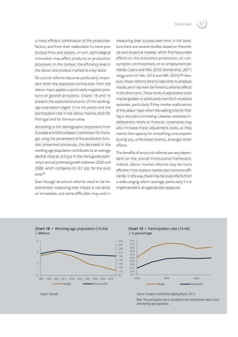
57Special issue

a more efficient combination of the production factors, and from their reallocation to more pro-ductive firms and sectors. In turn, technological innovation may affect products or production processes. In this context, the efficiency level in the labour and product markets is a key factor.

Structural reforms become particularly impor-tant when the expected contribution from the labour input applies a particularly negative pres-sure on growth prospects. Charts 18 and 19 present the expected evolution of the working-age population (aged 15 to 64 years) and the participation rate in the labour market, both for Portugal and for the euro area.

According to the demographic projections from Eurostat and the European Commission for Portu-gal, using the parameters of the production func-tion presented previously, the decrease in the working-age population contributes to an average decline close to -0.5 p.p. in the Portuguese econ-omy's annual potential growth between 2020 and 2080, which compares to -0.1 p.p. for the euro area.11

Even though structural reforms need to be im-plemented, measuring their impact is not direct or immediate, and some difficulties may exist in

measuring their success over time. In the litera-ture there are several studies, based on theoreti-cal and empirical models, which find favourable effects on the economy’s production, on con-sumption, on investment, or on employment (Al-meida, Castro and Félix, 2010; Gomes et al., 2011; Varga and in’t Velt, 2014 and IMF, 2015).12 How-ever, these reforms tend to take time to produce results, and may even be linked to adverse effects in the short term. These kinds of adjustment costs may be greater or particularly harmful in recessive episodes, particularly if they involve reallocations of the labour input when the waiting time for find-ing a new job is increasing. Likewise, excessive in-debtedness levels or financial constraints may also increase these adjustment costs, as they restrict the capacity for smoothing consumption during any unforeseen events, amongst other effects.

The benefits of structural reforms are very depen-dent on the overall institutional framework. Indeed, labour market reforms may be more effective if the product market also functions effi-ciently. In this way, there may be scale effects from a wide-ranging reform package, particularly if it is implemented in an appropriate sequence.

Chart 18 • Working-age population (15-64) | Millions

Chart 19 • Participation rate (15-64) | In percentage

90110130150170190210230250270

3

5

7

9

1985 1995 2005 2015 2025 2035 2045 2055 2065 2075


72.573.073.574.074.575.075.576.076.577.077.5

2020 2040 2060

Portugal Área do euro

Source: Eurostat. Source: European Commission (Ageing Report, 2017).

Note: The participation rate is calculated as the ratio between labour force and working-age population.


Box 4 | Potential output revisions

Potential output’s level and rate of growth are subject to particular uncertainty. This Box focuses on the difficulties associated with the estimation of contemporaneous values and the depen-dence on the dataset available.

In general, an estimate of potential output in real time may differ substantially from an estimate made thereafter under the same methodology, only due to the inclusion of new data that become available in the interim. To illustrate the magnitude of these revisions, Charts C.4.1 to C.4.4 show sequential estimates of potential growth and the output gap released by the European Commission13 and those that would result from the simple use of a Hodrick-Prescott filter (HP).14

Comparison between the initial and most recent estimates shows that the potential growth and the output gap are revised considerably in certain years. Furthermore, the revisions tend to be more significant in the output gap, as a result of the cumulative effect of the revisions on rates of change. The differences between the maximum and minimum values of the estimates for each year, represented by the white area, also confirm the degree of uncertainty, as the revisions do not always approximate to the most recent value. This is especially visible in the European Commission’s estimates for Portugal, where consecutive revisions are often observed moving in opposite directions.

The performance of the models is particularly affected during sharp cyclical shifts, when revisions tend to be very considerable. The period analysed includes very sharp revisions for Portugal,

Chart C.4.1 • Potential growth: HP filter | In percentage

Chart C.4.2 • Potential growth: European Commission | In percentage

-2.0-1.5-1.0-0.50.00.51.01.52.02.5

2008 2009 2010 2011 2012 2013 2014 2015

Initial estimate PTMost recent estimate PTInitial estimate EAMost recent estimate EA

-2.0-1.5-1.0-0.50.00.51.01.52.02.5

2008 2009 2010 2011 2012 2013 2014 2015


Sources: Banco de Portugal and Eurostat.

Notes: PT – Portugal; EA – Euro area. Annual estimates ba-sed on quarterly data. HP filter with a smoothing parameter of 7680, applied to quarterly data. The initial sample used to calculate the value for 2007 covers data from 1995-2008. This sample was extended sequentially by observations of 4 quarters up to 2016. The initial estimate of the HP filter for year t is based on a sample from 1995 to t+1. The most recent estimate is obtained using the complete sample of observed data (1995-2016). The white area represents the range between the minimum and maximum estimates for each year.

Source: European Commission.

Notes: PT – Portugal; EA – Euro area. The European Commis-sion estimates correspond to the spring forecasts published between 2008-2016. The initial estimate corresponds to the spring forecasts of t+1, when the GDP of period t is already observed. The most recent estimate corresponds to the spring 2016 forecasts. The white area represents the range between the minimum and maximum estimates for each year.

Special issue 59

given the persistence and severity of the recent recession. Although the euro area has not been immune to the recent international financial crisis, the revisions for this aggregate are compara-tively smaller.

On average, while the interval of estimates for potential growth over the period from 2008 to 2015 does not differ significantly when the estimates obtained through the HP filter are compared to those of the European Commission, this is not the case with the output gap. Taking the example of 2011, the output gap estimates produced by these two methodologies vary between -3.2% (European Commission) and 0.9% (HP filter). These results are particularly important when trying to establish the existence of any ’excess demand‛ (Box 2). In the case of the HP filter, potential output’s deviations from the actual values tend to be relatively less persistent. For example, it may be observed that the output gap is consistently negative from 2009, according to the European Commission’s estimates, while the HP filter estimates positive gaps for the years 2010, 2011 and 2015. A smoothing parameter of 7680 was used in this analysis, following Almeida and Félix (2006). In relative terms, these estimates reflect a smaller cyclical amplitude both for Portugal and for the euro area compared to the European Commission results. A smoothing parameter of 1600, which is more common in the literature, would result in less persistent business cycles, with a smaller amplitude, and a greater volatility of potential output, which would move more closely in line with actual GDP, impacting the revisions in the output gap.

The revisions of the estimates produced by the HP filter focus in particular on the end of the sample period (Charts C.4.5 and C.4.6), with the lengthening of the sample only resulting in

Chart C.4.3 • Output gap: HP filter | In percentage

Chart C.4.4 • Output gap: European Commission | In percentage

-7-6-5-4-3-2-101234

2007 2008 2009 2010 2011 2012 2013 2014 2015


-7-6-5-4-3-2-101234

2008 2009 2010 2011 2012 2013 2014 2015


Sources: Banco de Portugal and Eurostat.

Notes: PT – Portugal; EA – Euro area. Annual estimates based on quarterly data. HP filter with a smoothing parameter of 7680, applied to quarterly data. The initial sample to calculate the value for 2007 covers data from 1995 to 2008. This sample was extended sequentially by observations of 4 quarters up to 2016. The initial estimate of the HP filter for year t is based on a sample from 1995 to t+1. The most recent estimate is obtained using the complete sample of observed data (1995-2016). The shaded area represents the range between the minimum and maximum estimates for each year.

Source: European Commission.

Notes: PT – Portugal; EA – Euro area. The European Commis-sion estimates correspond to the spring forecasts published between 2008-2016. The initial estimate corresponds to the spring forecasts of t+1, when the GDP of period t is already observed. The most recent estimate corresponds to the spring 2016 forecasts. The shaded area represents the range bet-ween the minimum and maximum estimates for each year.


substantial changes to the estimates of the later years.15 In this exercise, the revisions at the end of the sample are significant, even when only the data observed for the extension period are used.

The European Commission’s estimates for remoter years are also revised considerably when new observations are added. These estimates are also subject to revisions resulting from any meth-odological changes and revisions in the actual data. In the case of the HP filter, this exercise only considers revisions to the trend component, given that the actual GDP series remains unchanged for all estimates.

In sum, potential output estimates are affected by the time of their calculation. Estimates in real time are provisional, and should be used with caution when analysing and defining economic pol-icy measures. The assessment of the business cycle and the economy’s potential growth requires the largest possible dataset, potentially sectoral, avoiding limited and partial sets that may lead to perception errors.

Chart C.4.5 • Mean revisions of potential output growth | In percentage points

Chart C.4.6 • Mean revisions of the output gap | In percentage points

0.0

0.2

0.4

0.6

-10 -9 -8 -7 -6 -5 -4 -3 -2 -1

HP PT CE PTHP AE CE AE

0.0

0.2

0.4

0.6

0.8

1.0

1.2

-10 -9 -8 -7 -6 -5 -4 -3 -2 -1

HP PT CE PTHP AE CE AE

Sources: Banco de Portugal, European Commission and Eurostat.

Notes: PT – Portugal; EA – Euro area. The figures reported are based on the mean absolute revisions for the period 1998-2015 vis-à-vis the most recent estimate (for the EC, spring 2016, in the case of the HP filter, the estimate obtained using the complete sample). The horizontal axis represents the num-ber of years elapsed between the estimated year and the year of the publication in the case of the EC and the year of the last observation included, in the case of the HP filter. HP filter with a smoothing parameter of 7680, applied to quarterly data. The initial sample covers data from 1995-2008, which was ex-tended sequentially by observations of 4 quarters up to 2016. The European Commission estimates correspond to the spring forecasts published between 2008-2016.

Sources: Banco de Portugal, European Commission and Eurostat.

Notes: PT – Portugal; EA – Euro area. The figures reported are based on the mean absolute revisions for the period 1998-2015 vis-à-vis the most recent estimate (for the EC, spring 2016, in the case of the HP filter, the estimate obtained using the complete sample). The horizontal axis represents the number of years elapsed between the estimated year and the year of the publi-cation in the case of the EC and the year of the last observation included, in the case of the HP filter. HP filter with a smoothing parameter of 7680, applied to quarterly data. The initial sample covers data from 1995-2008, which was extended sequentially by observations of 4 quarters up to 2016. The European Commission estimates correspond to the spring forecasts published between 2008-2016.

61Special issue

Final considerationsThe calculation of potential output is important for defining appropriate stabilisation policies. Despite the uncertainty inherent to the calcu-lation of this indicator, the output gap remains important for defining monetary and fiscal poli-cy in different economies, including in the euro area. The assessment of potential output is also relevant for the definition of policies with an impact on longer horizons. At these low fre-quencies, potential output growth is probably the most important variable for the determina-tion of economic well-being in a society.

The Portuguese economy faces a set of long-term challenges that require special attention. One of these challenges relates to demographic developments, both due to the expected decline in the working-age population, and due to their ageing. The projections available suggest a persistent negative impact of these factors on potential output. In contrast, the increase in skills based on growing education levels, result-ing from an education system that is adequate for the technological transformations in progress, may contribute to an increase in potential out-put for a prolonged period.

The increase in capital-per-worker levels is anoth-er important challenge. Correcting the high levels of indebtedness, in parallel with creating condi-tions that allow investment to increase, both in quantity and in quality, is essential for improving the Portuguese economy’s current position. The international financial crisis left significant marks in Portugal, particularly with regard to the condi-tions for accessing finance, with consequences for the accumulation of capital. Although there are no estimates available that link the sharp and persistent reduction of aggregate demand to the behaviour of aggregate supply, a topic that calls for discussion by the scientific community (Yellen, 2016), investment’s negative behaviour over a prolonged period will have repercussions on potential output.

An economy’s capacity to increase its poten-tial output is largely dependent on its legal and

institutional framework, namely the ability to cre-ate conditions that allow the most effective allo-cation of available resources possible. An insti-tutional restructuring designed to facilitate the emergence of competitive firms, as well as factor mobility between firms, may lead to a favourable creative destruction environment, increasing potential output. In contrast, the survival of firms with inferior performance, which remain active for longer periods than desirable, diverting pro-duction factors and financial resources, may hamper the economy’s restructuring process and limit economic growth (European Central Bank, 2011). The increase in economies’ com-petitiveness worldwide is one of the structural phenomena that should be taken into account when deciding on structural reforms, whether in the labour or product markets. According to available estimates for Portugal, one of the fea-tures of the recent buoyancy in economic activ-ity was the acceleration of total factor produc-tivity. It is vital over the medium term to design policies that support this trend.

This Special issue presented some of the main aspects associated with potential output, name-ly the concept, its role in economic analysis and the uncertainties inherent to its calculation. The topic will certainly continue to be the subject of debate and scrutiny in the literature and among the general public.


ReferencesAlichi, A., Bizimana, O., Laxton, D., Tanyeri, K., Wang, H., Yao, J., and F. Zhang, 2017, ’Multivari-ate Filter Estimation of Potential Output for the United States.‛ Working Paper 106, Interna-tional Monetary Fund.

Almeida, V., Castro, G. and R. Félix, 2010, ’Improv-ing competition in the non-tradable goods and labour markets: the Portuguese case.‛ Portuguese Economic Journal.

Almeida, V. and R. Félix, 2006, ’Computing Poten-tial Output and the Output Gap for the Portu-guese Economy.‛ Banco de Portugal, Autumn Economic Bulletin.

Amador, J., and C. Coimbra, 2007, ’Total Factor Productivity Growth in the G7 Countries: Differ-ent or Alike?‛ Working Papers w200709, Banco de Portugal.

Anderton, A. et al., 2012, ’Euro Area Labour Mar-kets and the Crisis.‛ Task Force of the Monetary Policy Committee of the European System of Central Banks, Occasional Paper Series No. 138.

Ball, L., Leigh, D., and P. Loungani, 2013, ’Okun’s law: fit at fifty?‛ NBER Working Paper 18668, National Bureau Of Economic Research.

Banco de Portugal, 2015a, ’European fiscal rules and the calculation of structural balances.‛ Special issue, October Economic Bulletin, Banco de Portu-gal, pp 85-106.

Banco de Portugal, 2015b, ’Demographic tran-sition and growth in the Portuguese economy.‛ Special issue, October Economic Bulletin, Banco de Portugal, pp 69-84.

Banco de Portugal, 2017a, ’International trade: gains and challenges.‛ Special issue, October Eco-nomic Bulletin, Banco de Portugal, pp 95-109.

Banco de Portugal, 2017b, ’Capital per worker and productivity.‛ Box 5.1, May Economic Bul-letin, Banco de Portugal, pp 59-61.

Barro, R., and X. Sala-i-Martin, 1995, Economic Growth, McGraw-Hill.

Blanchard, O., and J. Galí, 2007, ’Real Wage Rigidi-ties and the New Keynesian Model.‛ Journal of Money, Credit and Banking, Blackwell Publishing, vol. 39(s1), pages 35-65, 02.

Borio, C., Disyatat, F., and M. Juselius, 2013, ’Re-thinking potential output: Embedding informa-tion about the financial cycle.‛ BIS Working Pa-pers 404, Bank for International Settlements.

Bouthevillain, C., Cour-Thimann, P., Van Den Dool, G., Hernández de Cos, P., Langenus, G., Mohr, M., Momigliano, S., and M. Tujula, 2001, ’Cyclically adjusted budget balances: an alterna-tive approach.‛ European Central Bank working pa-per series no.77, September.

Bulligan, G., Busetti, F., Caivano, M., Cova, P., Fantino, D., Locarno, A., and L. Rodano, 2017, ’The Bank of Italy econometric model: an update of the main equations and model elasticities.‛ Working Paper 1130, Banca d’Italia.

Carabenciov, I., Ermolaev, I., Freedman, C., Kamenik, O., Korshunov, D., Laxton, D., Laxton, J., and M. Juillard, 2008, ’A Small Quarterly Multi-Country Projection Model.‛ IMF Working Paper No. 08/279, International Monetary Fund.

Centeno, M., Maria, J. and A. Novo, 2009, ’Unem-ployment: Supply, Demand, and Institutions.‛ In The Portuguese economy in the context of economic, financial and monetary integration, pp. 215–258. Banco de Portugal.

Christiano, L. J., Trabandt, M. and K. Walentin, 2011, ’Introducing financial frictions and unem-ployment into a small open economy model.‛ Journal of Economic Dynamics & Control, Vol 35, pp 1999-2041.

Del Negro, M., Hasegawa, R., and F. Schorfhei-de, 2016, ’Dynamic prediction pools: an investi-gation of financial frictions and forecasting per-formance.‛ Journal of Econometrics 192 (2016) 391–405.

Dias, F., Esteves, P. and R. Félix, 2004, ’Revisiting the NAIRU estimates for the Portuguese econ-omy.‛ Article, June Economic Bulletin, Banco de Portugal, pp. 39-48.

Draghi, M., 2017, Conference opening speech ’Structural reforms in the euro area‛, Frankfurt am Main, October.

European Central Bank, 2000, ’Potential output growth and output gaps: concept, uses and esti-mates.‛ Monthly Bulletin, October, pp 37- 47.

http://ideas.repec.org/a/mcb/jmoncb/v39y2007is1p35-65.html

http://ideas.repec.org/a/mcb/jmoncb/v39y2007is1p35-65.html

63Special issue

European Central Bank, 2011, Trends in poten-tial output, Monthly Bulletin, January, pp 73-85.

European Commission, 2017, ’The 2018 Ageing Report. Underlying Assumptions and projection Methodologies.‛ European Economy, Institutional Paper 065.

Galí, J., and J.D. López-Salido, 2000, ’A New Phil-lips Curve For Spain.‛ Documento de Trabajo nº 0109, Banco de España.

Galí, J., 2011, ’The return of the wage Phillips curve.‛ Journal of the European Economic Associa-tion, Vol. 9, No. 3, pp. 436–461.

Gomes, S., Jacquinot, P., Mohr, M., and M. Pisani, 2011 ’Structural reforms and macroeconomic performance in the euro area countries. A mod-el-based assessment.‛ Working Paper Series, No. 1323, European Central Bank.

Gordon, J. R., 2013 ’The Phillips Curve is Alive and Well: Inflation and the NAIRU During the Slow Recovery‛, NBER Working Paper No. 19390, National Bureau of Economic Research.

Havik, K., Morrow, K., Orlandi, F., Planas, C., Raci-borski, R., Röger, W., Rossi, A., Thum-Thysen, A., and V. Vandermeulen, 2014, ’The Production Function Methodology for Calculating Potential Growth Rates & Output Gaps.‛ Economic Papers 535, European Commission.

International Monetary Fund, 2015, ’Structural reforms and macroeconomic performance: ini-tial considerations for the fund.‛ Staff report.

Jorgenson, D.W. and K. Stiroh, 2000, ’Raising the Speed Limit: U.S. Economic Growth in the Information Age‛ Brookings Papers on Economic Activity, Vol. 1, pp 125-235.

Julio, P., e J. Maria, 2017, ’Output in the Portu-guese post-2008 period: A general equilibrium narrative.‛ Economic Studies, vol. 3, no. 2, Banco de Portugal.

Lafourcade et al., 2016, ’Labour market model-ling in the light of the financial crisis.‛ ECB Occa-sional Paper No. 175, European Central Bank.

Mankiw, G., 2003, Macroeconomics. Worth Pub-lishers.

Marcellino, M., and A. Musso, 2011, ’The reli-ability of real-time estimates of the euro area output gap.‛ Economic modelling, Vol.28, Issue 4, pp. 1842-1856.

Maria, J., 2016, 'Portugal: Trends, cycles, and instability in output and unemployment over 2008-2012.” Economic Studies, Vol II, No. 3, Ban-co de Portugal.

Martín-Moreno, J., Pérez, R., and J. Ruiz, 2010, ’Exploring the sources of Spanish macroeco-nomic fluctuations: An estimation of a small open economy DSGE model.‛ International Review of Economics and Finance, Vol 45, pp 417-437.

Murteira, B., Muller, D. and K., Turkman, 1993, Análise de sucessões cronológicas. Lisboa : McGraw Hill.

OECD, 2015, The Innovation Imperative: Con-tributing to Productivity, Growth and Well-Being, OECD Publishing, Paris.

Okun, A., 1962, ’Potential GNP: Its Measure-ment and Significance,‛ Cowles Foundation Paper 190, reprinted from the 1962 Proceedings of the Business and Economic Statistics Section of the American Statistical Association.

Orphanides A., and S. Norden, 2002, ’The unre-liability of output gap estimates in real time‛ The Review of Economics and Statistics, Vol.84, Issue 4, pp. 569-583.

Prachowny, M. F. J., 1993, ’Okun’s Law: Theoreti-cal Foundations and Revised Estimates.‛ The Review of Economics and Statistics, Vol. 75, No. 2, pp. 331-336.

Stiglitz, J.E., A. Sen and J.P. Fitoussi, 2009, Report of the Commission on the Measurement of Economic Per-formance and Social Progress, available at http://ec.europa.eu/eurostat/documents/118025/118123/Fitoussi+Commission+report.

Teles, P., and J. Garcia, 2016, ’How can the Phil-lips curve be used for today’s policy?‛, Economic Studies, Banco de Portugal, vol. 2, no. 2.

Varga, J. and J. in‘t Veld ,2014, ’The potential growth impact of structural reforms in the EU. A bench-marking exercise.‛ European Economy – Economic Papers, No. 541, European Commission.

Yellen, J.L., 2016, ’Macroeconomic research after the Crisis‛, speech at the conference ’The Elusive ‘Great’ Recovery: Causes and Implications for Future Business Cycle Dynamics’, Federal Reserve Bank of Boston, October.


Notes

1. Based on the Solow-Swan model, growth in steady state is closely related to the idea of long-term equilibrium of the economy, in which the various quan-tities grow at constant rates and where, consequently, key output ratios are stable (Barro and Sala-i-Martin, 1995; or Mankiw, 2003). For instance, the stock of capital increases at the same rate as GDP, whereby the capital-to-GDP ratio is constant. Inflation in the steady state is determined, for example, by the targets set by the central bank.

2. As an alternative, a production function could be considered with constant elasticity of substitution of factors, but not necessarily equal to 1, commonly referred to as CES (Constant Elasticity of Substitution).

3. A distinction should be made between the concept of natural output and that of ‘efficient output’, obtained under the assumption that the product and labour markets operate in perfect competition (see, for example, Blanchard and Galí, 2007).

4. Teles and Garcia (2016) use this definition of natural output. The authors identify a family of short-term Phillips curves that intersect a vertical long-term Phillips curve.

5. It has been suggested that this fact could be one of the reasons underlying technology’s small contribution to Portugal’s economic growth, in compari-son to other economies (Amador and Coimbra, 2007).

6. The uncertainties over use of potential output were approached for example in Orphanides and Norden (2002) and Marcellino and Musso (2011).

7. Jorgenson and Stiroh (2000) present estimates for the United States.

8. The 2018 Ageing Report: Underlying Assumptions & Projection Methodologies.

9. See for example the speech of Mario Draghi, President of the European Central Bank (18 October 2017).

10. It is important to note that GDP is sometimes criticised as a measure of social well-being. The need to value the inclusive aspect of economic growth has been emphasised by certain institutions, due to which the policymakers should also take into consideration equity in the distribution of the benefits of structural reform (see for example, OECD 2015). According to Stiglitz, Sen and Fitoussi (2009), substantial changes to the distribution of income may affect the use of GDP, or of any other per capita measure, as an indicator of households’ situation.

11. This calculation assumes an elasticity of 0.64 for GDP in relation to the labour input.

12. A very common exercise in general equilibrium models is to assess the effects of policies designed to increase the level of economies’ competitiveness, meaning those that lead to a narrowing of the gap between the costs borne by firms in producing goods and services and the prices actually paid by the users, whether final consumers or other firms.

13. The European Commission methodology is based on a production function and is described in Havik et al. (2014).

14. This filter is used in the Eurosystem exercises for the computation of the cyclically-adjusted budget balance (see Bouthevillain et al., 2001).

15. The magnitude and persistence of the impact of including additional information depend on the smoothing parameter chosen and therefore on the assumed duration of the business cycle.

economic bulletin - december 2017 - banco de portugal · economic bulletin | december 2017 ......

Documents