economic and policy implications of restricted patch...

Economic and Policy Implications of Restricted Patch Distribution

Karthik [email protected]

Mohammad S. [email protected]

Mohit [email protected]

January 7, 2013

Abstract

In this paper, we study how restricting the availability of patches to legal users impactsvendor’s profits, market share, software maintenance decisions, and welfare outcomes. Priorwork on this topic assumes that hacker’s effort is independent of the vendor’s decision to releasethe patch freely or not. Clearly, if the patch is not available to everyone, the hacker finds iteasier to exploit the vulnerability in the product and, as a result, is likely to alter his effort. Inorder to understand the role of a strategic hacker, we build a game-theoretic model, where thehacker’s decision is endogenous. With this model, we find that the hacker’s effort may, on onehand, decrease the utility that the vendor can extract from the consumers. On the other hand,it may help differentiate the legal version of the product from the pirated version. A vendorcan strategically exploit the hacker’s behavior in its pricing and software maintenance decisions.The endogeneity of hacker’s actions drives several of our findings that have interesting policyimplications. For example, the vendor may increase the price and reduce market share in orderto exploit the differentiation. In such a case, there may be more pirates in the restricted-patchcase than when the patch is freely available, a result that runs counter to typical argumentsprovided for restricting patches. A government body that understands this trade-off may exerta different level of piracy prevention effort so that the vendor is incentivized to make decisionsthat improve social welfare.

Key words : information security; patch distribution; countervailing incentive; public policy

1 Introduction

Software vendors have restricted the availability of patches only to legal users because of piracy

concerns. Windows Genuine Advantage from Microsoft is an example of such a program. Patch

restrictions also have implications on hackers’ efforts as they seek to exploit vulnerabilities that the

patches are designed to resolve. By restricting patch distribution, the vendor can indirectly control

the hacker’s action, which affects consumers’ expected utility and their buying decisions. Thus,

in addition to using the software price, vendor may use patch restriction to influence consumer

behavior. The impact of a strategic hacker on the resulting trade-offs has not been explored before.

Our aim is to derive managerial and policy insights by comparing two settings: one where patch

1

access is provided only to legal users and the other where patches are distributed freely (to both

legal users and pirates).

Patches can be categorized into two types (Lahiri, 2012): (a) Security updates which address

vulnerabilities that third party agents (e.g., hackers) exploit to compromise the software, and (b)

Performance updates which improve user experience (e.g., prevent system crashes). Because of

our focus on strategic interactions between the vendor and the hacker, we primarily study security

updates, although we briefly consider the performance updates later in the paper as well.

In order to limit piracy, government typically exerts effort by instituting laws, prosecuting of-

fenders, etc. So, a vendor’s decision to restrict updates is aimed at thwarting piracy above and

beyond the governmental effort. The hacker’s role in the market can be imagined as destroy-

ing/decreasing the consumer’s willingness to pay. So, at first glance, one would imagine that as

long as the marginal cost of effort in marginalizing the hacker is compensated by the corresponding

increase in the price of the software, the vendor will make the effort. However, that is not neces-

sarily the case. Our analysis finds that the hacker’s action has two different effects on the vendor

profit. The adverse effect–which is straightforward–decreases the consumer utility that the vendor

can extract and, therefore, has negative implications on the vendor profit. It occurs independent

of whether patches are restricted or not. The countervailing effect–which occurs only when the

patches are restricted–is one where the hacker’s actions are beneficial to the vendor profit. When

the latter effect is dominant, the hacker’s effort helps the vendor in further differentiating the legal

and the pirated versions of the software. So, it creates an incentive for the vendor to not marginalize

hacking activity, thereby improving the differentiation and, ultimately, his profit. This seemingly

counterintuitive behavior of the vendor has some interesting welfare implications as well.

The main argument that vendors provide in favor of restricting patch distribution is that it

encourages more of pirates to buy the software. However, we show that the vendor may increase

the price of the software while restricting patch distribution, in effect lowering the market share

and, in fact, increasing the incentive to pirate. Doing so, the vendor exploits the countervailing

effect of hacker actions that was alluded to earlier. This vendor behavior does not necessarily

reduce social welfare. Consider, for example, a situation where government exerts little antipiracy

effort. Then, a market may not be sustainable if distribution of patches is not restricted. We show

that the countervailing effect may provide enough differentiation via restricted patch distribution

2

that allows a vendor to serve the market and generate social welfare. Consequently, the hacker

may alleviate social planner’s investment in antipiracy measures. We also find that there may be a

disagreement between the social planner and the vendor regarding the policy of patch distribution

when the social planner is willing to put in moderate amount of effort in antipiracy effort levels.

The agreement is restored when the social planner is willing to exert significant antipiracy effort.

We deal with a parsimonious model involving two stages of strategic interactions. The vendor

makes the pricing and the software maintenance decisions in the first stage, and the hacker and

the users arrive at their decisions simultaneously in the second stage. Even for this stylized model,

where hacker actions are endogenized, a closed-form analytical solution to the vendor’s problem

seems intractable. Nevertheless, we develop various analytical insights using comparative statics

and numerical analyses.

This paper is organized as follows. In §2, we review the extant literature most relevant to this

topic. Following that, in §3, we describe our model. In §4, we present our equilibrium analysis and

§5 compares the two settings – one with no patch restriction and the other where patch distribution

is restricted. Finally, we present our concluding remarks in §6.

2 Literature Review

Our research relates to software maintenance, information security, and piracy literatures. We

provide a brief overview of each of these areas next. Towards the end of this section, we review two

specific papers–August and Tunca (2008) and Lahiri (2012)–in the literature that are most closely

related to the topic of our study.

In our model, the patch quality may be viewed as an outcome of the vendor’s software main-

tenance resource decision. We recognize that several papers have focused solely on the resource

allocation problem from various different perspectives. For example, Kulkarni et al. (2009) develops

a queuing model for optimal resource allocations. Similarly, Ji et al. (2005) consider the joint de-

termination of release time and the division of effort between constructing and debugging software

so that the total cost is minimized. Jiang and Sarkar (2003) analyzes the optimal software release

time where patching is explicitly considered and shows how the total cost can be reduced. To the

best of our knowledge, ours is the first paper to consider the resource decision along with patch

3

distribution policy restriction and its impact on piracy.

Our paper builds on extant literature on the economics of information security. Prior work has

analyzed various facets of this domain. Arora et al. (2004) shows that vulnerability disclosures

expedite the response from large vendors and subsequently benefit software users. Kannan and

Telang (2005) shows that a market-based mechanism for vulnerability disclosure makes the market

worse off than one without such a market. Arora et al. (2006) shows that a software vendor is

better-off releasing a buggier software early and patching it later particularly when the market

for the product is large. August and Tunca (2006) considers users’ incentive to patch security

flaws. They find that subsidy based patching policy performs better than mandatory or tax based

patching policy. Png and Wang (2009a) considers the strategic interaction between end-users in

taking security precautions and the interaction between end-users’ and hackers’ actions. Our paper

borrows several key modeling details from Kannan and Telang (2005). Different from the prior

information security literature, we investigate the possibility that the vendor uses the hacker’s

effort to improve his profit. We are not aware of any prior work that has focused on this aspect.

Our paper studies the patch restriction problem in the context of piracy. Most prior works on

software piracy analyze the impact of piracy on the legitimate producer’s sales and profit. A stream

of prior papers argue that a producer may not have the incentive to eliminate piracy from the market

(e.g., Chen and Png, 2003; Gopal and Sanders, 1997; Shy, 2001). For example, piracy generates

network externality benefits which may lead to increased demand for the legitimate version (Conner

and Rumelt, 1991; Shy, 2001). Pirated versions may also serve as a coordination device to reduce

price competition (Jain, 2008). Sharing may be profitable for the producer if the transaction cost

of sharing is lower than the marginal cost of production (Varian, 2000). The impact of piracy on

social welfare has been shown to cut both ways. Strict rules to combat piracy have been shown to

increase the producer’s profit while reducing the benefits of utilizing already developed products

(Chen and Png, 2003). Chen and Png (2003) contend that from the social welfare perspective, it

is better to manage piracy through price cuts than strict enforcement. Gopal and Gupta (2010)

suggest that bundling may have a deterrent effect on piracy. Different from these prior works, we

are more focused on restricting the patch distribution to pirates. Although we do not consider

network externality effects directly, we model the benefit of releasing patches freely in that this

policy diminishes hacker’s incentives to exert effort.

4

Our work is closely related to papers by August and Tunca (2008) and Lahiri (2012). August

and Tunca (2008) considers the patch restriction decision when the consumers exhibit negative

network effects due to piracy. They show that a vendor benefits from restricting patch distribution

to only legal users if the software is highly risky and antipiracy actions are mild, or the population’s

tendency to pirate is high. Lahiri (2012) considers a similar patch restriction problem but studies

how the positive versus negative network externality effects impact the overall outcome. He shows

that a strong positive network effect may require a less piracy-friendly and a more restrictive

patching strategy (i.e., restricting patches only to legal users). Both August and Tunca (2008)

and Lahiri (2012) rely on the presence of network effect to show the dominance of one policy over

the other. We do not impose any network effects but, unlike them, we consider hacker’s effort

endogenously. We show that this endogenous variation of hacker effort can lead to one policy being

dominant over the other. Our analysis on the impact of the hacker’s action on the vendor’s strategy

is unique.

3 Model

Our setup considers a two-stage game in a software market setting. We assume that the government

exerts an exogenously specified antipiracy effort of α ∈ [0, 1], where α = 0 implies that government

does not reduce pirate’s welfare and α = 1 implies that the government eliminates the pirate’s

welfare completely. It is reasonable to assume that government typically exerts at least some

antipiracy effort. So, for the analytical portion of the paper, we set α > 0. When numerically

conducting the comparative statics, we do so over the entire range of α, allowing α to be zero.

In the first stage, a monopolistic software vendor decides the price and resources to allocate

for software maintenance/patch development.1 These decisions, however, also depend on whether

or not the patch is made available to pirates. We analyze two variants of the two-stage game,

each corresponding to the patch distribution policy. Eventually we compare the optimal profits

obtained under the two patch distribution policies. In the second stage, a hacker and the users

simultaneously make decisions. The hacker decides on the effort exerted to exploit a vulnerability

in the software, and the users decide whether to buy or to pirate the software. Models such as

1Restrictions on patch distributions are relevant only in the context of a profit-maximizing vendor, which is whatis assumed here.

5

ours that consider one vulnerability and one hacker have been used to derive economic insights in

information security contexts before (see, for example, Kannan and Telang, 2005).

Next, we discuss the variables that model the decisions. We use a binary variable z to capture

whether the vendor distributes patches to pirates or not. When z = 1, the vendor makes the patch

available to all users, including the pirates; and, when z = 0, the patch is made available only to

legal users. In our analysis, we fix z a priori, which requires us to analyze the two cases separately.

Corresponding to each value of z, the vendor maximizes profit by optimally setting the price

and allocating resources to invest for patch development. We use p to denote the price set by the

vendor for the software. We assume as is reasonable that p ≥ 0. We capture the resources allocated

for maintenance using a proxy variable that measures the probability of successfully patching the

vulnerability in the software.2 Reasonably, there is a monotonically increasing relationship between

the aforementioned probability and the associated resource needs. The probability of fixing the

software is denoted by x, which must lie in [0, 1]. We assume that when x = 1, the provided patch

completely addresses the software vulnerability.

As mentioned above, in the second stage, both the users and the hacker make their decisions

simultaneously. A key factor that affects the user’s choice of whether to pirate or not is the

severity of the vulnerability in the software. We model this severity as the probability that a

successful exploitation of this vulnerability will render the user’s system inoperable. We denote

this probability by β, where β ∈ [0, 1]. This probability also measures the effort exerted by the

hacker in attacking the user’s system. Since there is a monotonic relationship between the hacker’s

effort and β, for simplicity of exposition, we let the hacker directly choose β. Therefore, β will be

referred to as the hacker’s effort. Note that we will later analyze the case when β is exogenously

chosen to highlight that the economic insights change substantially in this case. An exogenous β

may be a more appropriate choice for modeling performance updates.

2Even though the patch quality is typically realized only after the vendor allocates resources following the discoveryof a vulnerability, the sequence of decisions in our model captures the key effects of reality. The decision about howmuch of resources to allocate for maintenance is usually made even before the software is released. Furthermore, as inour model, the consumers usually take into account a vendor’s reputation for patching vulnerabilities before buying.Accordingly, we model the patch quality decision in the first stage.

6

3.1 Consumers and the Hacker

We model users (interchangeably, also referred to as consumers) along the lines similar to Kannan

and Telang (2005). Let the consumers in the market be heterogeneous in terms of the intrinsic value

they derive from the software. This consumer heterogeneity is captured by the variable θ ∈ [0, 1],

which is assumed to be distributed uniformly. We assume that the intrinsic value of the software

is θ2i for a user of type θi. Such a characterization is consistent with the reality where the number

of users having extremely large valuations is small and vice-versa. In our analysis, we deal with

market-share instead of the actual number of consumers that buy the product.

The consumer utilities and the surpluses may be different depending on whether they buy or

pirate the software (for example, if antipiracy efforts are strong or if patch distribution is restricted).

A legal user’s utility depends on the severity of the unpatched vulnerability β, and the patch quality

x.3 The term β(1−x) models the probability with which the user’s patched system is still rendered

inoperable. Therefore, a consumer of type θi has a utility of (1 − β(1 − x)) θ2i from buying the

software. So, her expected consumer surplus from buying the legal software is

CSb(θi) = (1− β(1− x)) θ2i − p. (1)

We model the pirated copy of the software as an inferior but vertically differentiated substitute

for the legal version. One factor that facilitates the differentiation is the government’s antipiracy

effort. The variable α is treated as the probability with which the pirated user may be subject

to legal actions. Hence, the government’s effort decreases a pirate’s utility by a factor of (1 − α).

Such a depiction of the government’s antipiracy effort on a pirate’s utility is similar to Baea and

Choi (2006). The other factor that differentiates the legal and the pirated copies is the limit

imposed by the vendor on patch distribution. When the patch is available only to legal users, a

pirate is expected to suffer more from the vulnerability than when there is no such restriction. We

capture this aspect by characterizing the probability that a pirate’s system is rendered inoperable

as β(1−xz). Assuming a zero cost for procuring the pirated version, the consumer surplus for type

3We make the assumption that all users, if available, apply the patch update. This reflects the recent advancementsin patch distribution and application.

7

θi from pirating is:

CSp(θi) = (1− β(1− x z)) θ2i (1− α). (2)

Notice that α serves to vertically differentiate the legal version from the pirated version independent

of the value of z, whereas β serves to vertically differentiate only when z = 0. Observe that consumer

utility terms within the CSb(θi) and CSp(θi) expressions are bounded from above by one. Also,

CSp(θi) is non-negative. We use θ to denote the highest consumer type that pirates the software.

We make a few remarks about θ and its properties. First, by the assumption on the consumer

heterogeneity, θ is naturally bounded between zero and one. Second, θ exists since the consumer

with θi = 0 pirates. Third, CSb(θ)−CSp(θ) ≤ 0. Fourth, a consumer of type θi buys the software

if and only if θi > θ because CSb(θ) − CSp(θ) is a non-decreasing function of θ. In other words,

we may say that there exists a θ such that consumers of type θi ∈ [0, θ] pirate the product and

consumers of type θi ∈ (θ, 1] buy the product.

Next, we focus on the decision problem faced by the hacker. Recall that β is a consequence

of a hacker’s strategic actions to discover and exploit the vulnerability. The notion of a strategic

hacker has critical implications for the analyses, as we will discuss later. The benefit that the

hacker gains from exploiting a system is characterized in a manner similar to Kannan and Telang

(2005). The hacker gains are proportional to θi if he successfully breaks into the system of a user of

type θi. Of course, the probabilities of breaking-in may differ for the pirated and the legal versions.

This probability is simply β(1 − x) for the legal version and β(1 − xz) for the pirated one. Let

the hacker’s cost be C(β). Since consumers of type [0, θ] pirate and the rest buy the product, the

following models the expected payoff for the hacker:

πh(β) = β(1− x z)∫ θ

0θ dθ + β(1− x)

∫ 1

θθ dθ − C(β).

We use a logarithmic cost function for the effort: C(β) = −M log(1 − β), where M > 0 is an

exogenous parameter. The functional form is reasonable and chosen to model that, as β increases,

increasing marginal efforts are required to effect the same increase in the probability of finding a

vulnerability. In particular, the limiting conditions are that the hacker incurs an infinite cost to

discover the vulnerability with certainty but incurs no cost when exerting no effort. The hacker’s

8

decision problem is supβ∈[0,1] πh(β).

Lemma 1. Given θ and L, there exists an ε > 0, such that supβ πh(β) is attained at a β∗ in

[0, 1− ε].

Given that the hacker keeps β∗ < 1, we now characterize the highest consumer type that pirates

the software, denoted above as θ. Let κ(α, β, x, z) = (1− β)α+ βx(1− z + zα). It is easy to check

that 0 < κ(α, β, x, z) ≤ 1 because α ∈ (0, 1], β ∈ [0, 1), x ∈ [0, 1] and z ∈ {0, 1}. Note that

the difference in the utilities from buying and pirating the software for a consumer of type θi is

κ(α, β, x, z)θ2i . Since κ(α, β, x, z) > 0, all consumers with θi > 0 derive a strictly higher utility from

purchasing the software when compared to pirating it. In short:

θ = min

{√p

κ(α, β, x, z), 1

}. (3)

3.2 Vendor Profit Function

The revenue for the vendor from selling the software is p(1− θ). Let K(x) denote the cost incurred

for improving the patch quality. Assuming zero marginal cost for producing software, the vendor’s

profit is: π(x, p) = (1− θ)p−K(x) and his decision problem is sup(x,p)∈[0,1]×[0,∞) (1− θ)p−K(x).

We again assume a logarithmic cost function K(x) = −L log(1 − x) for the effort, where L > 0

is exogenous. Observe that the cost function is reasonable. In particular, when x = 1, the cost

is infinity, which can be interpreted to say that the vendor cannot completely secure the system.

Similarly, if the vendor does not exert any effort, the cost is zero.4

We show that it suffices to impose p ≤ κ(α, β, x, z) by resetting the price, whenever the above

condition is violated, without altering the strategies of any of the players in any practically relevant

manner. In particular, if in an equilibrium p > κ(α, β, x, z) then the vendor may instead set

p = κ(α, β, x, z) and achieve the same profit because θ = 1. Further, in that case, hacker’s decision

does not depend on p. Therefore, the equilibrium is for all practical matters the same and although

the price is reduced, no one buys the product so none of the objective values or decisions change.

4An earlier version of this work motivated a similar cost function in Png and Wang (2009b).

9

Since p may be restricted to be no more than κ(α, β, x, z):

θ =

√p

κ(α, β, x, z). (4)

Lemma 2. There exists an optimal solution (x∗, p∗) to the vendor’s decision problem such that

π(x∗, p∗) > 0, x∗ ≤ 1 − exp(− 1L

)< 1, and 0 < p∗ < κ(α, β, x∗, z) ≤ 1. Correspondingly,

0 < θ∗ < 1.

Therefore, the vendor’s decision problem is max(x,p)

{π(x, p)

∣∣ (x, p) ∈[0, 1− exp

(− 1L

)]× [0, 1]

}.

4 Equilibrium Analysis

We compute the equilibria by considering the two-stage games that are obtained by setting z =

1 and z = 0 separately. For each game, we compute the Subgame Perfect Nash Equilibrium

(Fudenberg and Tirole, 1991) by solving the second stage first. We solve the second stage game

in a generic manner, i.e., for both z values. As regards the first stage, it turns out that the

equilibrium computations and analyses are straightforward when z = 1. However, for z = 0,

the first stage equilibrium seems intractable. Despite this limitation, we analytically demonstrate

several interesting results and supplement them with insights gained through numerical analyses.

We first focus on the second stage which constitutes a simultaneous game between a hacker and

consumers where the players decide respectively on the level of hacking effort and whether or not

to buy the software. In the proof, we use a technical property of certain types of functions, that

we refer to as single-crossing functions.5

Definition 3. A function h(u) : R 7→ R single crosses another function g(u) : R 7→ R from above

(respectively, below) if, for all u′′ > u′, h(u′) − g(u′) ≤ 0 implies that h(u′′) − g(u′′) < 0 (resp.,

h(u′)− g(u′) ≥ 0 implies that h(u′′)− g(u′′) > 0).

Intuitively, the above definition captures the property that the graphs of two functions intersect

at no more than one point. First observe that if, as per Definition 3, h(u) single crosses g(u) from

above then h(u) and g(u) can intersect at at most one point. To see this, assume that h(u′) = g(u′)

5Note our definition is different from the manner in which the single crossing property is associated with Spence-Mirlees condition in economics.

10

and h(u′′) = g(u′′). Without loss of generality let u′ < u′′. Then, the definition above requires

that h(u′′) < g(u′′) which is in contradiction of our hypothesis. Next, note that if h(u) − g(u) is

a continuous function, h(u) − g(u) is positive and negative for some values of u, and h(u) does

not equal g(u) at more than one point then h(u) single crosses g(u) from above or from below.

Assume that h(u) equals g(u) only if u = u. Then, because of continuity, and by exchanging g

and h if necessary, we may assume without loss of generality that h(u) − g(u) > 0 for u < u and

h(u)− g(u) < 0 for u > u. Then, we show that h(u) single-crosses g(u) from above. Consider any

u′ such that h(u′)− g(u′) ≤ 0. Then, u′ ≥ u and therefore, for all u′′ > u′, h(u′′)− g(u′′) < 0. The

proof for the second stage solution exploits the following technical lemma which captures a simple

property of the single crossing functions.

Lemma 4. Assume for every i ∈ I, h(u) single crosses gi(u) from above (resp. below), then h(u)

single crosses maxi∈I gi(u) from above (resp. below).

Now, we are ready to prove the uniqueness of the solution to the second-stage game.

Lemma 5. The equilibrium second stage variables are obtained by solving the simultaneous equa-

tions involving (3) and

β = max

{1− 2M

1− x(1− (1− z)θ2

) , 0} (5)

The resulting solution {θ∗, β∗} is unique, β∗ < 1, and also, ∀ M ∈ [12 ,∞], β∗ = 0.

We make significant use of the uniqueness of {θ∗, β∗} in deriving our results. We remark that

although the techniques used in the proof of Lemma 4 depend on the functional forms, they do so

primarily by exploiting the strict monotonicity of√

pκ(α,β,x,z) and 1 − 2M

1−x(1−(1−z)θ2 and the fact

that they satisfy the single-crossing property defined above. We will build on these aspects later.

The lemma shows that when M ≥ 12 , there is no hacker effort (i.e., β∗ = 0) for either z.

Consequently, (3) is independent of z and as a result the patch quality x or price p does not depend

on z either. So, the prices, profit, welfare outcomes are the same and the policy comparison becomes

uninteresting. To focus on the interesting cases, we restrict M to be less than 1/2 hereafter. The

following subsections deal with the first stage decisions for each patch distribution policy, i.e., value

of z, separately.

11

4.1 Patch available to all users (z = 1)

In this section, the vendor makes the patch available to everybody. Setting z = 1, we obtain from

(4) and (5) that:

{β∗, θ∗} =

{max

{1− 2M

1− x, 0

}, min

{√p

α(1− β∗(1− x)), 1

}}. (6)

Observe that since patches are made available to everybody, the hacker’s payoff is independent of

the share of the market that buys the product. Consequently, β∗ expression is independent of θ∗.

To simplify the notation we denote (β∗, θ∗) as (B,Θ) in the remainder of this section. Then, Θ∗

and B∗ respectively denote the untapped market and the hacker effort at the price p∗ and patch

quality x∗ that yields maximum profit for the vendor. In the following π∗v denotes the maximum

profit of the vendor. Using the above expressions in the vendor’s decision problem, we compute

the equilibrium:

Proposition 6. The equilibrium market share for the vendor is 13 ; the corresponding decisions for

the vendor and the hacker are:

{p∗, x∗, B∗} =

{1

9(8Mα), 0, 1− 2M

}L ≥ 4α

27{1

9(8Mα+ 4α− 27L),

4α− 27L

4α, 1− 8αM

27L

}4α27 ≥ L >

8αM27{

4α

9, 1− 2M, 0

}8αM

27 ≥ L > 0;

and the vendor profits are

π∗v =

8Mα

27L ≥ 4α

27

8Mα

27+

4α

27− L+ L log

(27L

4α

)4α27 ≥ L >

8αM27

4α

27+ L log(2M) 8αM

27 ≥ L > 0.

Notice from Proposition 6 that there are three regions where an equilibrium may occur. When

the cost for the quality of patch is sufficiently high, i.e., L ≥ 4α27 , the vendor does not have an

incentive to develop a patch, i.e., x∗ = 0, and the equilibrium is straightforward. When the cost

of the hacker’s effort is large relative to vendor’s effort M > 27L8α (which is same as, 8αM

27 > L), the

12

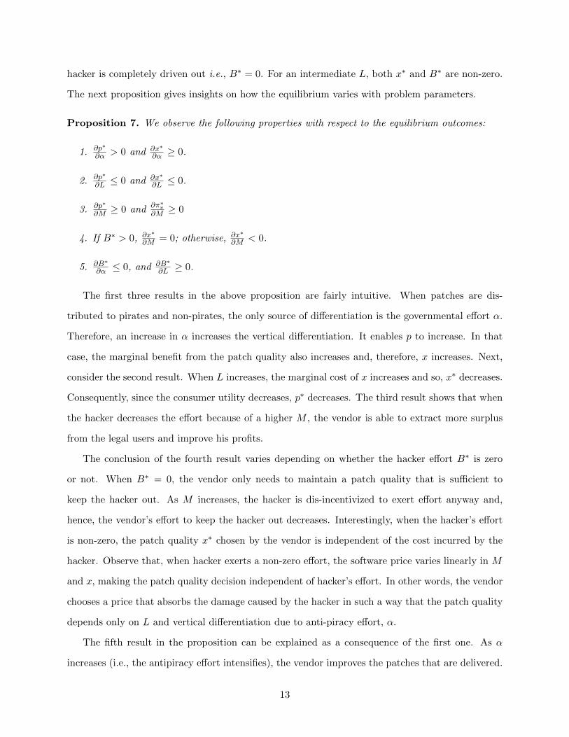
hacker is completely driven out i.e., B∗ = 0. For an intermediate L, both x∗ and B∗ are non-zero.

The next proposition gives insights on how the equilibrium varies with problem parameters.

Proposition 7. We observe the following properties with respect to the equilibrium outcomes:

1. ∂p∗

∂α > 0 and ∂x∗

∂α ≥ 0.

2. ∂p∗

∂L ≤ 0 and ∂x∗

∂L ≤ 0.

3. ∂p∗

∂M ≥ 0 and ∂π∗v

∂M ≥ 0

4. If B∗ > 0, ∂x∗

∂M = 0; otherwise, ∂x∗

∂M < 0.

5. ∂B∗

∂α ≤ 0, and ∂B∗

∂L ≥ 0.

The first three results in the above proposition are fairly intuitive. When patches are dis-

tributed to pirates and non-pirates, the only source of differentiation is the governmental effort α.

Therefore, an increase in α increases the vertical differentiation. It enables p to increase. In that

case, the marginal benefit from the patch quality also increases and, therefore, x increases. Next,

consider the second result. When L increases, the marginal cost of x increases and so, x∗ decreases.

Consequently, since the consumer utility decreases, p∗ decreases. The third result shows that when

the hacker decreases the effort because of a higher M , the vendor is able to extract more surplus

from the legal users and improve his profits.

The conclusion of the fourth result varies depending on whether the hacker effort B∗ is zero

or not. When B∗ = 0, the vendor only needs to maintain a patch quality that is sufficient to

keep the hacker out. As M increases, the hacker is dis-incentivized to exert effort anyway and,

hence, the vendor’s effort to keep the hacker out decreases. Interestingly, when the hacker’s effort

is non-zero, the patch quality x∗ chosen by the vendor is independent of the cost incurred by the

hacker. Observe that, when hacker exerts a non-zero effort, the software price varies linearly in M

and x, making the patch quality decision independent of hacker’s effort. In other words, the vendor

chooses a price that absorbs the damage caused by the hacker in such a way that the patch quality

depends only on L and vertical differentiation due to anti-piracy effort, α.

The fifth result in the proposition can be explained as a consequence of the first one. As α

increases (i.e., the antipiracy effort intensifies), the vendor improves the patches that are delivered.

13

This increase in patch quality decreases the marginal payoff that hacker obtains. Hence, the decrease

with respect to α. A similar reason explains why B∗ increases as L increases.

4.2 Patch available to legal users only (z = 0)

In this section, we consider the case where the vendor makes the patch available only to the legal

users. Set z = 0 in (3) and (5) to see that the second stage equilibrium is obtained as a solution of:

{β∗, θ∗} =

{max

{1− 2M

1− x(1− θ∗2), 0

}, min

{√p

α− β∗(α− x), 1

}}. (7)

Earlier when z = 1, β∗ was independent of θ∗ and as a result, the vendor’s decision problem was

relatively straightforward to solve in closed-form. In the above equation, however, because the

expression for β∗ involves θ∗ and vice-versa, the vendor’s decision problem does not seem to have

a simple closed-form solution. This makes the ensuing analysis somewhat more complicated.

Given α, x, and M , we show that we may construct an invertible relation between p and θ∗.

First observe that Lemma 4 shows that, given a p, there is a unique θ∗ that solves (7). Now, we

consider the reverse direction and obtain p as a function of θ∗. Given a θ∗ < 1, p can be easily

computed using (7) since β∗ is a function of θ∗, M , and x which are all available. Now, consider

the case when θ∗ = 1. Clearly, the price is not uniquely determined in this case. However, we

recall that when θ∗ = 1, setting p = κ(α, β, x, 1) does not change the equilibrium in any practically

relevant way (see discussion prior to Lemma 2). Furthermore, the vendor sets the price in a way

such that θ∗ is strictly less than 1. Therefore, we set p = κ(α, β∗, x, 1) when θ∗ = 1, realizing that

there is no equilibrium at which p ≥ κ(α, β∗, x, 1). It follows that the mapping between p and θ∗ is

invertible.

The primary advantage of the invertible mapping between p and θ∗ is that it allows us to

interpret the vendor’s action as choosing (x, θ∗) instead of (x, p). This is particularly important

since expressing θ∗ as a function of p is unwieldy, whereas the inverse mapping is easy to express.

As before, we denote (β∗, θ∗) as (B,Θ) in the remainder of this section. We have also restricted

14

the domain of x based on Lemma 2. With these transformations, the vendor’s problem reduces to:

max(x,Θ)∈[0,1−exp(− 1

L)]×[0,1]

π′v(x,Θ) =

(1−Θ)Θ2α+ L log (1− x) if x > 1−2M(1−Θ2)

(1−Θ)Θ2

((α− x)

2M

(1− (1−Θ2)x)+ x

)+L log (1− x)

otherwise

(8)

Observe that the condition x > 1−2M(1−Θ2)

corresponds to the case when B = 0. Further, when

x = 1−2M(1−Θ2)

, evaluating any of the expressions on the right-hand-side yields the same value. We

denote the optimal solution to (8) as (x∗,Θ∗), the corresponding price as p∗ and the equilibrium

effort of the hacker as B∗.

Lemma 8. x∗ 6> 1−2M1−Θ∗2 . If B∗ = 0, then x∗ = 1−2M

1−Θ2 and Θ∗ ≤ 23 .

Lemma 8 shows that, when the hacker does not exert effort, i.e. B∗ = 0, the vendor will choose

the minimum patch quality that is needed to keep the hacker from exerting any effort. The lemma

also allows us to further restrict the domain of x to[0, 1−2M

1−Θ2

]. This reformulates (8) into the

following optimization problem:

max(x,Θ)

L log (1− x) + (1−Θ)Θ2

(2M(α− x)

(1− (1−Θ2)x)+ x

)

0 ≤ x ≤ min

{1− exp

(− 1

L

),1− 2M

1−Θ2

}0 ≤ Θ ≤ 1

(9)

Since x ≤ 1 − exp(− 1L

)< 1, it follows that the objective function is continuous over the feasible

region, which in turn is compact. Therefore, it follows from Weierstrass Theorem that there exists

an optimal solution to (9), a consequence which also follows from Lemma 2.

This specification also makes it clearer why it is hard to solve the vendor’s problem in closed-

form. Although it might appear at first glance that the intractability is due to the logarithmic

cost function of x, it is in fact still difficult to optimize the objective of (9) with respect to Θ

when x is fixed. To see this, fix x in (9) and maximize vendor profit with respect to Θ. Then,

the first order optimality condition of the objective function with respect to Θ yields a fifth order

polynomial equation. We show in the next example that this observation is at the heart of why

15

vendor’s problem is difficult to solve in closed-form.

Example 9. According to Abel-Rufini’s theorem, there does not exist a generic algebraic solution

to polynomial equations of degree five or higher. In fact, Galois’ Theory sharpens Abel-Rufini’s

theorem by showing that a polynomial is solvable in radicals if and only if the associated Galois

group is solvable. When one chooses M = 111 , α = 1

2 , and x = 14 , the first order optimality

condition with respect to Θ reduces to the solution of

33Θ5 − 22Θ4 + 206Θ3 − 132Θ2 + 369Θ− 246 = 0. (10)

Since the associated Galois group is not solvable, the roots of this polynomial equation cannot be

expressed exactly with radicals. We are particularly interested in the root Θ that lies in [0.66, 0.67].

It can be verified using Sturm’s theorem that there is exactly one such root. Observe that ∂πv(x,Θ)∂Θ

does not depend on L. On the other hand, a change in L impacts the optimal patch quality x∗.

We now show that there exists an L ∈[

110 ,

111

]such that

(x = 1

4 ,Θ = Θ)

satisfies the first order

optimality conditions for (9). First, let L = 110 . It is easy to verify that dπv(x,Θ)

dx

∣∣∣x= 1

4

has the same

sign as −165Θ7 + 165Θ6 − 750Θ5 + 728Θ4 − 1245Θ3 + 1113Θ2 − 198 which, by Sturm’s theorem,

is negative for all Θ ∈ [0.66, 0.67]. Therefore, dπv(x,Θ)dx

∣∣∣x= 1

4,Θ=Θ

< 0 when L = 110 . Similarly, when

L = 111 , it can be shown that dπv(x,Θ)

dx

∣∣∣x= 1

4,Θ=Θ

> 0. Since dπv(x,Θ)dx

∣∣∣x= 1

4

is a continuous function

of L, there exists an L such that(

14 , Θ

)satisfies first order optimality conditions for (9). In

fact, it can be verified numerically (within tolerances) that this solution is the optimal decision for

the vendor. Numerical verification here is reasonable since it can be shown that there are a finite

number of points that satisfy the local optimality conditions. This was done by verifying, using

Sturm’s theorem, that the leading terms of a Groebner basis of the polynomials obtained from the

first order optimality conditions do not vanish in the specified range of L. Since we have argued

that Θ cannot be expressed exactly using radicals, this example shows that there is little hope for

closed-form solutions to the vendor’s problem when patches are restricted to legal users.

Although we shall not be able to express the optimal solution in closed-form, we expose various

interesting properties of the solution. Recall that, by Lemma 2, we may restrict Θ ∈ (0, 1). For a

given Θ ∈ (0, 1), we denote the optimal patch quality as x∗(Θ). Similarly, given x, we denote the

16

optimal untapped market as Θ∗(x). By Weierstrass Theorem, it can be easily verified that these

optimal solutions exist.

Theorem 10. 1. Given Θ ∈ (0, 1), x∗(Θ) is unique and decreasing in M . For L ≥ 427 , x∗ = 0.

2. Let Θ′ ∈ Θ∗(x). If x = α then Θ′ = 23 . If x > α, Θ′ > 2

3 . Finally, consider x < α. If

x ≤ 95(1− 2M) then Θ′ = 2

3 . Otherwise, Θ′ < 23 .

3. ∃{α,L} such that for M = M , x∗ = α and B∗ 6= 0. Further, there exists an ε such that if

M = M + ε (resp. M = M − ε) then x∗ < α (resp. x∗ > α) and B∗ 6= 0.

Arguably, Theorem 10 is the most important result that enables us to derive analytical insights

from the model. The reader may find the details of the proof interesting. In particular, consider

Point #3 of Theorem 10. Although it is reasonably straightforward to show that(α, 2

3

)satisfies local

optimality conditions for the vendor’s optimization problem for some settings of the parameters,

this is not sufficient to prove Point #3 because the vendor’s objective is not concave (as illustrated

in Figure 1(a)). Therefore, it is necessary to check global optimality of this decision for the vendor.

The main trick in the proof is the construction of a nonconvex overestimator for the vendor’s

objective over the relevant region for which we establish using semialgebraic geometry tools that(α, 2

3

)is the global optimum. Then, because the overestimator exactly estimates the vendor’s

objective at(α, 2

3

), the result follows.

Using Point #1, L can be bounded for numerical computations. This result in conjunction

with Proposition 6 shows that if L ≥ 427 then x∗ = 0 regardless of the patch distribution policy.

Then, Θ, B, p are also independent of z because the consumer surplus does not depend on z. The

comparisons are therefore uninteresting in this case and we restrict L ≤ 427 hereafter.

The insights from the above theorem are interesting in several ways. First, observe that Point

#2 shows that the optimal solutions have an interesting and somewhat counterintuitive, structure.

In particular, when x∗ is large, the market tapped is small and vice-versa. This is because when

the vendor exerts significant effort towards improving the patch quality, it also increases the price

significantly so that the market share is reduced. This structure can also be seen from Figure 1(b).

Second, as mentioned earlier, the vendors’ argument for limiting the availability of patches is that

the patch restrictions encourage more users to buy legal versions. In contrast, Points #2 and #3

17

(a) Concavity of the vendor profit (b) Solution space Θ × x: The marked area is where thesolution can fall in

Figure 1: Figures to explain Theorem 10

in Theorem 10 show that sometimes (specifically M < M) fewer consumers buy the software when

patch is restricted in distribution. This result shows that the vendor does not limit patches simply

to target the pirates but may strategically restrict patches to improve profits by extracting more

surplus from the legal users.

Point #3 leads to the following theorem:

Theorem 11. For certain values of (α,M,L), the vendor profit increases with M and, for certain

others, it decreases. In other words, ∂π∗v

∂M is sometimes positive and other times negative.

At the outset, one might expect that the hacker effort decreases vendor profit because an

increased hacker effort decreases consumer surplus which the vendor uses to extract a profit. This

obvious effect will henceforth be referred to as the adverse effect of hacker’s effort on vendor’s

profit. However, Theorem 11 shows that that an increase in hacker’s effort may allow the vendor

to extract more profit. This happens because an increase in B can help vertically differentiate the

legal version from the pirated version of the software. When the patch is only distributed to legal

users, the hacker is incentivized to exert more effort, which diminishes a pirate’s utility more than

it reduces a legal user’s utility. In effect, the hacker makes the legal version more valuable for the

consumers, which allows the vendor to charge a higher price to generate more profit. We refer to

18

this effect as the countervailing effect of hacker’s effort.

We now explain, in an intuitive manner, the primary effects that drive some of the results derived

in Theorems 10 and 11. First observe that the vendor’s profit increases when more users purchase a

legal copy of the software, i.e., when Θ reduces. Since Θ =√

pα−B(α−x) , the effect of hacker’s effort,

B, on Θ and hence on vendor’s profit depends on the sign of α−x∗. More specifically, if α > x∗, i.e.,

when government exerts significant antipiracy effort, Theorem 10 shows that Θ∗ < 23 , i.e., vendor’s

share is more than 13 . Observe that hacker’s effort decreases monotonically with increase in his cost

parameter M . Then, a decrease in hacker’s effort or, equivalently, an increase in M , results in a

decrease in Θ and thus an increase vendor’s profit. However, when α < x∗, i.e., government does

not exert significant antipiracy effort, an increase in hacker’s effort or equivalently a reduction in

M , leads to a decrease in Θ when p is fixed and therefore increases vendor’s profit. Interestingly,

despite this tendency of Θ to increase for a given price, we show in Theorem 10 that the vendor

sets a price such that Θ∗ > 23 and the resulting market share is strictly less than 1

3 . In other words,

the vendor is able to exploit the countervailing effect of hacker and takes advantage of the vertical

differentiation between legal and pirated software arising from hacker’s efforts.

4.2.1 Numerical Analysis

Note that all the relevant parameters are bounded: α ∈ [0, 1] by model specification; Lemma 5 and

Theorem 10 provide bounds on M and L, respectively; the endogenous variables Θ, B, and x are

each in the range [0, 1] by model construction; Lemma 2 further restricts x and p; and the same

lemma establishes existence of an optimal solution to the vendor’s problem. Since vendor’s profit is

continuous (see Equation 9), we explore the solution space by constructing a grid of points within

the above bounds.

As before, we denote the optimal price by p∗, patch quality by x∗, vendor profit by π∗, untapped

market by Θ∗, and hacker effort by B∗. Unless specified otherwise, it is assumed that these solutions

correspond to the case when the patches are restricted in distribution to the legal users. Figure 2

shows how p∗ and x∗ vary with respect to L and α. The variations are similar to those when z = 1

(see Proposition 7) and so are the explanations. Next, consider the variation of x∗ and π∗ with

respect to M . When x∗ < α (see Figures 3(d)-3(f)), the corresponding profits in Figures 3(a)-3(c)

increase with M , which one may recall as the adverse effect described after Theorem 11. However,

19

(a) Variation with respect to α(M = 0.05, L = 0.01)

(b) Variation with respect to L (α =0.5, M = 0.05)

Figure 2: Effect of Antipiracy Effort and Cost of Patch Quality.

when α < x∗, it can be observed in the same figures that profits decrease with an increase in M

because of the countervailing effect.

Our numerical analysis also shows that patch quality does not increase as M increases (see

Figures 3(d), 3(e), and 3(f)). In some cases, the vendor does not exert any effort on patch quality,

i.e., x∗ equals zero (see Figure 3(f)). In contrast, in other settings, the vendor provides a sufficient

patch quality to drive the hacker out i.e., B∗ = 0). In this case, x∗ is maintained at the level

necessary to keep the hacker marginalized. In Figure 3(e), we observe a kink at the value of M

beyond which x∗ is maintained at the minimum level necessary to keep the hacker from exerting

effort B∗ = 0.

Next, consider the variation of price and market-share with M . When the countervailing effect

is dominant, the vendor appears to always decrease p∗ as M increases. Since both the price as

well as the patch quality can influence the type of consumer that is indifferent, the market share

variations are not monotonic. These can be seen in Figures 3(k), 3(h), 3(l), and 3(i). In contrast,

when the adverse effect is dominant, both the price and the market-share vary non-monotonically

with M . When the adverse effect is dominant, for the lower range of M , the price cut is insufficient

to make up for the decreased differentiation and, the market share continues to fall. However, for

slightly larger M , the price cut makes up for the decreased differentiation and the market-share

improves. These can be seen in Figures 3(j), 3(g), 3(l), and 3(i).

We make the following observations based on the numerical analysis:

Numerical Observation 12. • The optimal patch quality decreases as M increases.

20

(a) Optimal Profit: α = 0.10,L = 0.01

(b) Optimal Profit: α = 0.95,L = 0.01

(c) Optimal Profit: α = 0.50,L = 0.05

(d) Patch Quality: α = 0.10,L = 0.01

(e) Patch Quality: α = 0.95,L = 0.01

(f) Patch Quality: α = 0.50,L = 0.05

(g) Optimal Market Share: α =0.10, L = 0.01

(h) Optimal Market Share:α = 0.95, L = 0.01

(i) Optimal Market Share: α =0.50, L = 0.05

(j) Optimal Price: α = 0.10,L = 0.01

(k) Optimal Price: α = 0.95,L = 0.01

(l) Optimal Price: α = 0.50,L = 0.05

Figure 3: Effect of M on Optimal Price, Profit, Market Share, and Patch Quality

• Within a certain range of L, whenever M = Mx=α = (9−5α)(4−4α−27L)72(1−α) (resp. M = Mx=0 =

9(4−27L)8(9−5α) ), the equilibrium is attained when x∗ = α (resp. x∗ = 0) and Θ∗ = 2

3 .

21

Observe that a partial proof of the second numerical observation can be obtained by adapting

the proof of Theorem 10. To see this, observe that the settings of the parameters in the proof:

α = 12 , L = 1

18 , and M = 13144 satisfy the relation M = (9−5α)(4−4α−27L)

(72(1−α)) . Whenever M satisfies the

above relation,(α, 2

3

), it is easy to check that

(α, 2

3

)satisfies the local optimality conditions because,

at this point, the partial derivative of πv(x,Θ) is zero with respect to both variables. Moreover, it

was shown that the derivative of πv(x∗(Θ),Θ) is never zero elsewhere. Since the coefficient of the

associated polynomials are continuous functions of α, L, and M , it follows that small perturbations

of these parameters do not alter the difference of the number of sign changes of the Sturm Sequence

over the intervals used in the proof since the roots do not occur at the end-points. Therefore, even

when small perturbations are made to {α,L,M} in such a way that M = (9−5α)(4−4α−27L)(72(1−α)) , the

optimal solution remains(α, 2

3

).

5 Comparative Statics

This section focuses on comparing the equilibrium outcomes and welfare implications under the

two patch distribution policies, i.e., with z = 1 versus z = 0. The first subsection compares the

equilibrium values of p∗, x∗, B∗, and Θ∗, whereas the second one analyzes the corresponding social

welfare generated. Like in the previous section, we establish some of the results analytically while

others are found via numerical computations.

As before, we deal with α 6= 0 in the analytical portion of the subsections below. When dealing

with α = 0 in the numerical portion, the discussion that follows will be relevant. The consumer

utilities from buying and pirating can be the same when α = 0. If the consumer utilities from

buying and pirating are the same then either p = 0 or p > 0 and no one buys the software. In

either case, the vendor does not have any revenue or profit. So, the market may not exist in such

cases. If z = 1 then α = 0 is necessary and sufficient for the utilities to be the same (and the

market to not exist). If z = 0 then α = 0 is necessary but not sufficient. Here, in addition to α = 0,

the versions cannot be differentiated only if either B∗ = 0 or x∗ = 0.

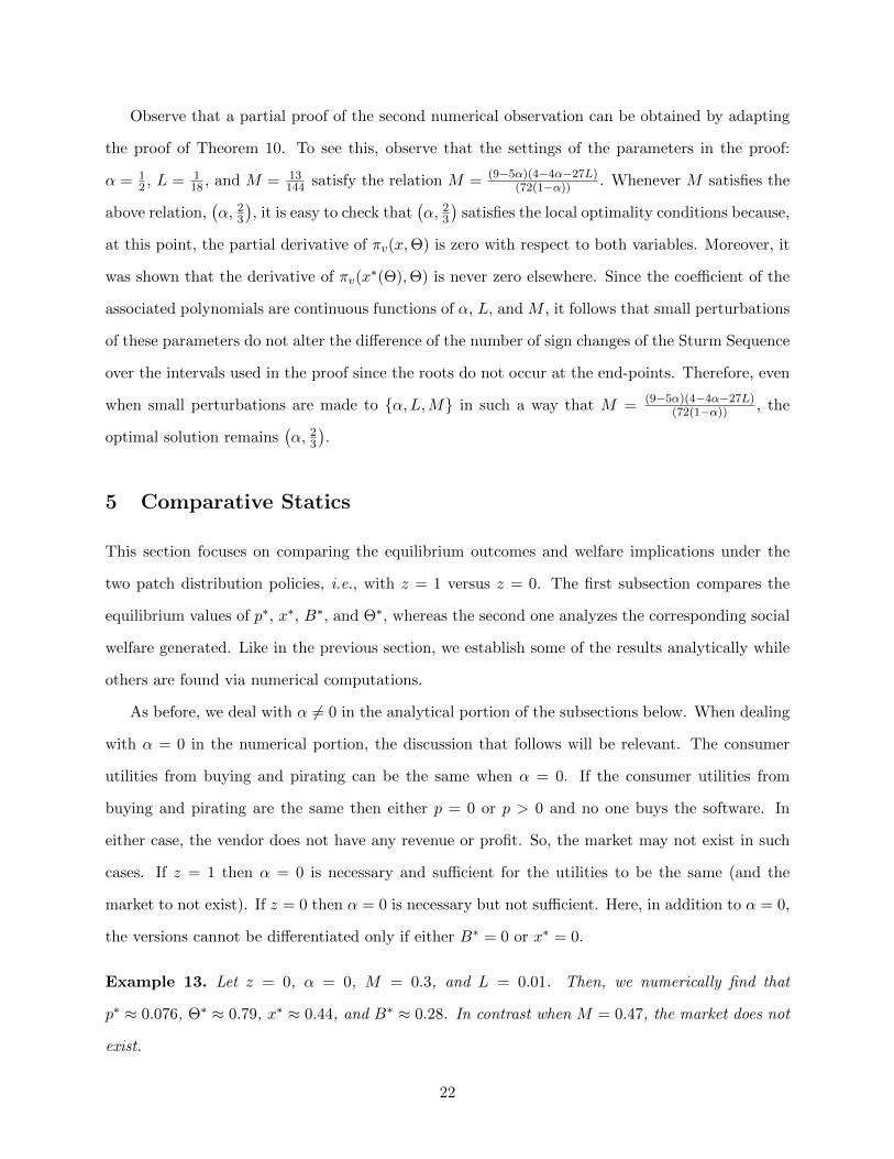
Example 13. Let z = 0, α = 0, M = 0.3, and L = 0.01. Then, we numerically find that

p∗ ≈ 0.076, Θ∗ ≈ 0.79, x∗ ≈ 0.44, and B∗ ≈ 0.28. In contrast when M = 0.47, the market does not

exist.

22

5.1 Comparison of p∗, x∗, π∗, B∗, and Θ∗

We first compare vendor’s profit under the different patch distribution policies. To fix notation, we

denote the value of z as a subscript. For example, p∗0 (resp. p∗1) is the optimal price when patches

are restricted in distribution (resp. freely available).

Proposition 14. There exists an α such that, for all α ∈ [α, 1], the equilibrium vendor profit is

strictly higher when patches are released to everyone compared to when patches are restricted in

distribution.

The above result shows that the vendor may have a larger profit by releasing the patch to

everyone in comparison to adopting the restricted patch distribution policy. This seemingly counter-

intuitive result can be explained as follows. When government puts a large antipiracy effort, there

is not much value for pirates and, as a result, the product is already vertically differentiated.

Unpatched pirated copies increase the incentive of the hacker to exert effort and this action takes

away consumer surplus from legal users as well which the vendor could have extracted as profit.

Instead, the vendor offers the patches to everyone leaving anti-piracy efforts to the government,

thereby discouraging hackers and extracting the higher surplus from its consumers.

We next show that the vendor will choose to distribute the patches to all the users only if the

hacker’s action is endogenous. For this purpose, we diverge from the model specification proposed

in this paper and regard β as exogenous.

Proposition 15. If β is exogenously specified (not decided by the hacker as a strategic variable)

the equilibrium is such that θ = 23 regardless of the patch distribution policy. Further, it is never

strictly optimal for the vendor to release the patch to everyone.

As discussed before, we can consider exogenous β as modeling the case of performance updates

because, in this setting, hacker’s action does not depend on the quality of the update. For such

updates, if the vendor restricts the distribution of the patch, while maintaining the same price and

patch quality, then more consumers have an incentive to purchase the legal copy of the software

since performance updates increase the software’s utility. To take advantage of this fact, the vendor

increases the price, still serves the same fraction of the market, and earns a higher profit. It follows

that it is never strictly better for the vendor to release performance updates freely. We remark

23

that the analytical difficulty of deriving the equilibrium solution is significantly reduced when β

is exogenous. In this case, closed-form solutions are amenable because the second-stage game is

simple. Moreover, the structure of the solution is also less rich when β is exogenous. In particular,

with exogenous β, the vendor targets 13rd of the market regardless of the patch distribution strategy.

Notwithstanding, when β is endogenous and patches are restricted in distribution, the vendor may

target a smaller or larger market share in the equilibrium strategy.

(a) Price (M = 0.05, L = 0.01) (b) Price (M = 0.25, L = 0.01) (c) Price (M = 0.35, L = 0.05)

(d) Profit (M = 0.05, L = 0.01) (e) Profit (M = 0.25, L = 0.01) (f) Profit (M = 0.35, L = 0.05)

Figure 4: Comparative Statics - Effect of α.

We now revert back to the case of endogenous hacker action, which is more appropriate for

security updates, and analyze the model using numerical computations. Figure 4 shows the vari-

ation of profits and prices with α. For low values of α, the vendor prefers to restrict patches and

vice-versa. When α = 0, the market cannot exist with unrestricted patches (z = 1) but the vendor

may be profitable for z = 0 by exploiting the countervailing effect (see Example 13 for a specific

scenario). This tendency to exploit the hacker’s effort to differentiate the two versions and obtain

higher profits continues even for slightly larger α values. With an increase in α, the incentive of the

vendor to employ the hacker’s effort to differentiate the versions decreases. Consequently, vendor

continues to restrict the patch until a threshold α and thereafter releases the patch freely. The

24

threshold α decreases as M increases. This can be explained because, as M increases, the hacker’s

effort reduces and the vendor’s reliance on the countervailing effect decreases. The price variations

in the figures can also be similarly explained.

(a) Hacker’s Effort (M = 0.05,L = 0.01)

(b) Hacker’s Effort (M = 0.25,L = 0.01)

(c) Hacker’s Effort (M = 0.35,L = 0.05)

(d) Patch Quality (M = 0.05,L = 0.01)

(e) Patch Quality (M = 0.25,L = 0.01)

(f) Patch Quality (M = 0.35,L = 0.05)

Figure 5: Optimal Hacker’s Effort and Patch Quality - Effect of Antipiracy Effort(α).

Next, we consider Figure 5, which depicts the variation of B∗ with respect to α. As α increases,

the number of pirated copies available for exploit decreases for both cases of patch distribution

policy and, so, the hacker’s effort, B∗, also decreases for both settings of z. The key difference is

in the pace at which B∗ decreases – the decrease is faster when z = 1. The difference in the rate

of decrease can be attributed to the vendor’s incentive to preserve the hacker when z = 0 for its

countervailing effect on the consumers.

Lastly, consider the variation of x∗ in Figure 5. When α = 0, there is no differentiation for

z = 1 and x∗1 = 0; but x∗0 may not be zero because the vendor takes advantage of the countervailing

effect to differentiate legal software from its pirated counterpart. For small enough α values, the

same trade-offs occur leading to a better patch quality when z = 0. The rate at which patch quality

increases with an increase in α is faster when patches are available freely relative to when they are

25

restricted in distribution. This behavior can also be attributed to the vendor’s incentive to drive

the hacker out quickly when only the adverse effect is present. The following remark summarizes

the aforementioned observations:

Numerical Observation 16. 1. For low values of α, the vendor profit and the price are higher

for z = 0 compared to that for z = 1.

2. The hacker is driven out (i.e., B∗ = 0) at a lower value of α when z = 1 than when z = 0.

3. The rate at which the patch quality increases is higher when z = 1 than when z = 0.

5.2 Social Welfare

This section compares the social welfare generated. Defining social welfare in our context requires

care because it must be decided whether the welfare of the pirate and/or the hacker should be

included in social welfare. Building on Trumbull (1990), we choose to exclude hacker’s welfare but

include the net benefits of all users and the vendor in our definition of social welfare. The payments

from the users to the vendor are transfers, which cancel out in our calculations. Accordingly, the

social welfare is:

SW =

Indeterminate if α = 0 and

z = 1, or

z = 0 and (x∗ or B∗) = 0

(1−B∗(1− x∗ z)) (1− α)

∫ Θ∗

0θ2 dθ

+(1−B∗(1− x∗))∫ 1

Θ∗θ2 dθ + L log(1− x∗)

otherwise

The first case deals with scenarios when there is no differentiation between the legal and the pirated

versions. Also, as mentioned in Section 3, we do not consider the strategic role of the social planner

and, hence, we do not include the cost of α in the social welfare expression. In the following, we

primarily focus on studying how the social welfare varies with α.

Setting z = 0 and z = 1 in the social welfare expression we obtain SW0 and SW1. Figure 6 shows

the variation of social welfare with α under both cases. Consider first z = 1, in conjunction with

the corresponding variations in B∗ and x∗ in Figure 5. When α is so small that x∗1 = 0 or x∗1 is large

enough that B∗1 = 0, the social welfare decreases as α increases because pirates lose the surplus

26

(a) Social Welfare (M = 0.05,L = 0.01)

(b) Social Welfare (M = 0.25,L = 0.01)

(c) Social Welfare (M = 0.35,L = 0.05)

Figure 6: Social Welfare.

due to the (1 − α) term. When x∗1 6= 0 and B∗1 6= 0, there exists a range of α values where social

welfare increases with α. This may be explained as follows. As anti-piracy efforts increase, fewer

consumers pirate the software, which reduces the incentive of the hacker to exert effort, increasing

the utility for both legal and pirate users. Beyond a certain threshold, the intense antipiracy effort

decreases the surplus of the pirates drastically and, consequently, the social welfare decreases even

when B∗1 6= 0. (e.g., Figures 6(b) and 6(c)).

The social welfare under z = 0 has a more monotonic relationship with α. As noted when

studying the equilibrium properties, the patch quality monotonically increases with α. This im-

proves the surplus of the legal users. However, the surplus of the pirates decreases due to increasing

α. Taken together, the overall social welfare decreases monotonically.

Interesting insights can be derived by comparing the two cases. When the antipiracy effort is

low, it may not be possible for the vendor to sustain presence if the patches are distributed freely,

i.e., z = 1. Clearly, in this case, social welfare is higher when z = 0. As α increases, although

the hacker effort aids the vendor via the countervailing effect, it also diminishes the social welfare

of the society. Hence, for moderate α values, the welfare from z = 1 is better. This may play an

important role in policy considerations.

Numerical Observation 17. 1. The threshold α value at which the vendor prefers to release

patches freely (i.e., his profits are higher with z = 1) is larger than the value of α when the

social planner prefers the vendor to do so.

2. When there is little antipiracy effort, strategically exploiting hacking activity by restricting

27

access to the patch to only legal users can be social welfare improving.

3. Maximum social welfare is obtained when a moderate level of antipiracy effort is exerted and

the vendor is required to release the patch freely.

The first point in the above observation leads us to believe that the vendor does not necessarily

have an incentive to freely release patches even though doing so maximizes social welfare. Instead, a

government regulation may be required to make this happen. However, as the second point argues,

such a regulation has to be complemented with an appropriate level of antipiracy effort. If sufficient

antipiracy effort is not exerted, the society may again be worse off. This is because markets that

fail in the presence of the regulation may sustain in an unregulated environment where the vendor

is allowed to adopt a restricted patch distribution policy. Thus, our observations point to the need

for complementing regulations with an appropriate level of antipiracy effort.

6 Discussions and Conclusion

Software vendors are taking an active role in thwarting piracy by restricting access to patches. This

paper studies the implications of the vendor’s decision to restrict patch distribution. Specifically,

our interest is in analyzing how the vendor can exploit the strategic role of a hacker in order to

maximize his profits. We employ a relatively simple model that has a reasonable level of fidelity.

Nevertheless, analytical closed-form solutions describing the equilibrium strategy of the players

in this game-theoretic model do not seem amenable. Despite this shortcoming, we demonstrate

various results analytically and complement them with a thorough numerical analysis.

We identify two main effects of the hacker’s activity on the vendor profit. The adverse effect,

which occurs independent of the vendor’s decision to restrict the patch, decreases the welfare of

the legal users that the vendor can extract. In contrast, the countervailing effect differentiates the

legal and pirated versions of the software when the patches are restricted and is therefore liked

by the vendor. Whether the adverse or the countervailing effect dominates depends respectively

on whether the patch quality is lower or higher than the governmental antipiracy effort. We

demonstrate the interesting interplay between antipiracy efforts, patch distribution policies, and

patch quality decisions on the vendor profits.

28

Our analysis finds that the countervailing effect has many interesting implications. We demon-

strate that the often-cited motivation for restricting patch, i.e., to increase market-share, is not

necessarily valid when the countervailing effect is dominant. In such a case, we found that the

vendor may decrease the market-share, exert more effort in providing good quality patches, and

charge a higher price to generate more profit. Next, we present some policy insights arising from

our analysis and also compare them against prior works.

The countervailing effect helps sustain the market in some cases. If the governmental antipiracy

effort is low, the countervailing effect provides the only vertical differentiation that the vendor can

use to serve the market. Stated differently, the presence of the hacker is beneficial to the market

as a whole when the cost of hacking is low and the government wishes to invest little resources.

There are also differences between when the vendor and the social planner prefer to make the

patch available to everyone. The government prefers that the patch be made available freely for

moderate levels of antipiracy effort. The vendor only does so for a higher level of antipiracy effort.

So, to achieve the best social welfare outcomes, the government has to choose an appropriate level

of antipiracy effort and also require the vendor to release the patch to all users.

To the best of our knowledge, related prior works in the literature have not considered the

countervailing effect. As we demonstrated in Proposition 15, if the hacker action is not endogenized,

the vendor always prefers the restricted patch distribution policy. Instead, if hacker action is

endogenized the vendor may have sufficient incentive to release patches freely when the government

exerts sufficient antipiracy effort (see Proposition 14). Further, if hacker action is not endogenized,

the vendor always targets 13rd of the market and we do not see the situation where the vendor

improves patch quality and increases price to target a smaller segment of consumers. In August and

Tunca (2008) and Lahiri (2012), features such as network externality generate the differentiation

between the restricted patch and no restricted patch scenarios. As a consequence, some of the

comparative statics results observed are different compared to our model. For example, August

and Tunca (2008) find cases when the intense antipiracy enforcement should be complemented with

the decision to restrict the patch distribution. However, that issue does not arise in our context.

The next obvious question is: how robust are our results to relaxing various assumptions,

including the uniform distribution of consumers, the functional form of consumer and the hacker

utilities, etc.? To address this question, we provide features of the model that are critical to

29

establishing the results. If the probability terms used in Equations 1 and 2 are retained the same

but the functional form of the consumer utility/demand is made more general, the indifferent

consumer type will continue to include a term (x−α). This is the term that drives the main results

in our paper about the countervailing versus the adverse effect trade-off. As one may realize, the

term will continue to play a similar qualitative role even in a generic setting although the second

order effects from the generic functions may affect the specific values. If one were to pay careful

attention to the proofs, an important feature of the model is the single-crossing property of Lemma

4, which helps establish the uniqueness of B and Θ. Another important feature of the model for

analytical results is that the first partial derivative of vendor’s profits is a rational function that

enables us to use semialgebraic geometry tools for the analysis. Once we discovered the results of

Theorems 10 and 11, we found that they have quite intuitive explanations that primarily depend on

how β interacts with (x−α) (see discussion after Theorem 11). We also performed some numerical

computations with other monomial utility functions for consumer types and found that the results

we derived extend to those settings as well. For these reasons, we conjecture reasonably confidently

that our results should be valid more generally.

Although our results provide interesting insights regarding the implications of restricted patch

distribution, our analysis is not without limitations. The key limitation of our study is that some

of the insights were derived through numerical computations, which were performed by creating

a grid with a granularity of 0.01 for the problem parameters. In Example 9, we provided some

justification for our approach. Second, in our model we assume that if the patch is available to the

user, the user will patch the system. However, this may not be the case. Thirdly, implementing the

restricted patch distribution policy need not be costless. Incorporating these features, performing

analytical investigations with more general cost and utility functional forms would be interesting

avenues for further research. Further, it would be interesting to investigate if the results found in

our analysis can be validated empirically.

30

A Proofs

A.1 Proof of Lemma 1

Since πh(0) = 0, it follows that supβ πh(β) = supβ{πh(β) | πh(β) ≥ 0}. However,

β(1− x z)∫ θ

0θ dθ + β(1− x)

∫ 1

θθ dθ ≤ β(1− xz)

∫ 1

0θ dθ ≤ β(1− xz)

2≤ β

2

Therefore, any β such that πh(β) ≥ 0 satisfies C(β) ≤ β2 ≤

12 . In other words, for a given L, there

exists an ε > 0 such that β ≤ 1− ε. For a given θ, πh(β) is continuous over [0, 1− ε]. Therefore, by

Weierstrass theorem, supβ πh(β) is attained at some β ≤ 1− ε.


First note that because κ(α, β, x, z) ≤ 1, we have already argued that any equilibrium can be

represented with a software price that is less than or equal to one. Define S = [0, 1) × [0, 1] and

Πv = supx,p{π(x, p) | (x, p) ∈ S}. Since (0, 0) ∈ S, it follows that Πv ≥ 0. Let S′ = {(x, p) |

π(x, p) ≥ 0}. It follows that Πv = supx,p{π(x, p) | (x, p) ∈ S′}. We now show that S′ is compact.

If (x′, p′) ∈ S′, then L log(1 − x′) ≥ −1. Let S′′ =[0, 1− exp

(− 1L

)]× [0, 1]. Then, S′ ⊆ S′′. It

is easy to verify that π(x, p) is continuous over S′′ and therefore S′ = S′′ ∩ {(x, p) | π(x, p) ≥ 0}

is compact. Using Weierstrass Theorem, it follows that the supremum in the definition of Πv is

attained. Let the optimal solution to the vendor’s problem be (x∗, p∗). We have shown in the

discussion before the lemma, that p∗ may be restricted to lie in [0, κ(α, β, x∗, z)]. We now argue

that p∗ ∈(0, κ(α, β, x∗, z)

). We proceed by contradiction. First note that if p is set at any of

the boundary points the vendor revenue is 0 and therefore π(x∗, p) = 0. We show that there

exists another solution (x′, p′) such that π(x′, p′) > 0. Let x′ = 0 and p′ = κ(α, β, x∗, z)/2. Since

κ(α, β, x∗, z) > 0, p′ > 0 and it can be easily verified that θ < 1. Therefore, π(x′, p′) > 0. Since

p∗ ∈(0, κ(α, β, x∗, z)

)it follows that θ ∈ (0, 1).


Consider u′ such that h(u′) − maxi∈I gi(u′) ≤ 0 and u′′ > u′. Let i be such that gi(u

′) =

maxi∈I gi(u′). Then, h(u′′) − maxi∈I gi(u

′′) ≤ h(u′′) − gi(u′′) < 0, where the second inequality

31

follows since h(u) single crosses gi(u) from above by definition.


By Lemma 1, let β∗ = arg maxβ hπ(β). Now, by Fermat’s theorem, β∗ ∈{

0, β = 1− 2M1−x(1−(1−z)θ2)

}.

Observe that πh(β) > πh(0) = 0. If β > 0 then β∗ = β else β∗ = 0. Therefore, the equilibrium

solution (θ∗, β∗) is obtained by solving (3) and (5) simultaneously for θ and β. Since M > 0 and

1−x(1− (1− z)θ2) ≥ 0, it follows that if the equilibrium is attained at (θ∗, β∗) then β∗ < 1, which

was also shown in Lemma 1. Finally, if M ≥ 12 , then β < 0. Therefore, β∗ = 0.

We now prove that there is a unique solution to (3) and (5). When z = 1 or x = α, it can

be trivially shown that (3) and (5) intersect at a unique point given x, α, p, and M . This is

because in the former case (5) is independent of θ and if z = 0 and x = α then (3) does not depend

on β. Therefore, we assume for the remaining proof of uniqueness that x 6= α and z = 0. Let

r(β) =√

pα(1−β)+βx . If p = 0, it is easy to show that there is a unique solution to (3) and (5).

Therefore, we may assume p > 0 and consequently θ∗ > 0. Since x 6= α, it follows that r(β) is

strictly monotone in β and therefore invertible. By direct calculation, r−1(θ) = − pθ2(α−x)

+ αα−x .

Since r(β) is strictly monotone, r−1(θ) is strictly monotone in θ. Let s(θ) = 1 − 2M1−x(1−θ2)

and

define w(θ) = r−1(θ)− s(θ). Then:

w(θ) = r−1(θ)− s(θ) =−p+ px− pxθ2 + xθ2 − x2θ2 + θ4x2 + 2Mθ2α− 2Mθ2x

θ2(α− x)(1− x+ xθ2)

We show that there do not exist θ′, θ′′ ∈ (0, 1], θ′ 6= θ′′, such that w(θ′) = w(θ′′) = 0. It is easy to

verify that the denominator of w(θ) is non-zero when θ ∈ (0, 1]. Replace u = θ2 and observe that

the numerator is negative when u = 0. Further, as u increases, the numerator becomes positive

because either x > 0 in which case the coefficient of u2 is positive or x = 0 in which case the

coefficient of u2 is zero and the coefficient of u is 2Mα, which in turn is strictly positive. Since the

numerator is quadratic in u, it has at most one root in (0, 1]. Therefore, w(θ) has at most one root

in (0, 1]. Since r−1(θ) and s(θ) are continuous, it follows that, for θ ∈ (0, 1], r−1(θ) single-crosses

s(θ) either from above or below. Further, since r−1(θ) is strictly monotonic, it is easy to verify that

if r−1(θ) crosses s(θ) from above (resp. below) then it also crosses the identically zero function

from above (resp. below). The former occurs when α < x and the latter when α > x. Then, it

32

follows from Lemma 4 that r−1(θ) crosses max{0, s(θ)} either from above or below.

Let S1 = {(min{r(β), 1}, β) | 0 ≤ β ≤ 1} and S2 = {(θ,max{0, s(θ)}) | 0 ≤ θ ≤ 1}. We now

show that S1 ∩ S2 is a singleton. Assume that α < x. Then, r−1(θ) single-crosses max{0, s(θ)}

from above and r−1(θ) is strictly monotonically decreasing. Now consider points (θ, β) ∈ S1

such that r(β) ≥ 1. Clearly, θ = 1. Also, observe that as θ approaches ∞, r−1(θ) approaches

αα−x , which in turn is negative. It follows as a result that all points of the form (1, β), where

0 ≤ β ≤ min{r−1(1), 1}, belong to S1. Observe that there is only one element in S2 such that

θ = 1. Then, S1 intersects with S2 at such a point if and only if min{r−1(1), 1} ≥ max{0, s(1)}.

Since max{0, s(1)} < 1, the condition reduces to r−1(1) ≥ max{0, s(1)}. However, as shown

above, r−1(θ) single-crosses max{0, s(θ)} from above. This implies that r−1(θ) > max{0, s(θ)} for

θ < 1. In other words, if α < x, S1 ∩ S2 is a singleton. Now, consider the case when α > x.

In this case, r−1(θ) crosses max{0, s(θ)} from below and is monotonically increasing. Further,

as θ approaches ∞, r−1(θ) approaches αα−x , which is at least one. Therefore, points of the form

(1, β) belong to S1 if and only if 1 ≥ β ≥ max{r−1(1), 0}. Such a point belongs to S2 if and only

if max{0, s(1)} ≥ max{r−1(1), 0} which is equivalent to r−1(1) ≤ max{0, s(1)}. However, since

r−1(1) crosses max{0, s(1)} from below, this implies that r−1(θ) < max{0, s(θ)} for θ < 1. In other

words, if α > x, S1 ∩ S2 is a singleton. Therefore, the uniqueness of (θ∗, β∗) is proven.

A.5 Proof of Proposition 6

We consider the decision variables p and x separately. First note that by Lemma 2, we may assume

that p < κ(α, β, x, 0) and that, given x, B is independent of p. Therefore, we solve for p first: p∗ =

4αmin{2M+x,1}9 . The first order optimality conditions fix Θ∗ = 2

3 . Then, by Lemma 2, the vendor’s

decision problem for deciding patch quality reduces to max{πv(x) | x ∈

[0, 1− exp

(− 1L

)]}, where

πv(x) = 4αmin{2M+x,1}27 +L log (1− x). For x > (1−2M), it is easy to check that πv(x) < πv(1−2M)

because the first term is constant and the second term is strictly decreasing. Consequently, we may

additionally restrict x to [0, 1−2M ]. Observe that the πv(x) is strictly concave in x and, therefore,

the optimal patch quality is unique. Further, express πv(x) as 4α(2M+x)27 +L log (1− x) and observe

that it is differentiable w.r.t. x. It is easy to verify that πv(0) > 0 ≥ πv(1− exp

(− 1L

)). So,

by Fermat’s theorem, x∗ ∈{

0, 1− 27L4α , 1− 2M

}. (Note that 1 − 2M > 0 since M < 1

2 .) The

proposition lists the various cases that occur depending on which value of x maximizes vendor’s

33

profit.

A.6 Proof for Lemma 8

We first show that x∗ ≤ q(Θ) = 1−2M1−Θ∗2 . Assume for deriving a contradiction that x∗ > q(Θ∗) and

the corresponding software price is p∗. Then, it follows from (7) that B∗ = 0. Now consider the

situation where the vendor chooses the patch quality x′. Observe from (7) that the equilibrium

market share is independent of x when hacker is not exerting an effort. Therefore, the corresponding

equilibrium solution to the second stage problem is (β∗, θ∗) = (0,Θ∗). It follows from the definition

of π′v(x,Θ) (see (8)) that πv(x′,Θ∗) > πv(x

∗,Θ∗). Therefore, (x∗,Θ∗) does not maximize πv(x,Θ)

contradicting our assumption.

Now, we prove the last statement of the result. If B∗ = 0, then it follows from the above

argument that x∗ ≤ q(Θ∗). However, B∗ = 0 implies that x∗ ≥ q(Θ∗). Therefore, x∗ = q(Θ∗). It

is easy to check that (1 − Θ)Θ2α is a decreasing function for Θ ∈[

23 ,∞

]. Further, since M < 1

2 ,

L log(1− x) is a decreasing function of Θ if x = q(Θ). Therefore, Θ∗ ≤ 23 .

A.7 Proof for Theorem 10

Proof for Point #1: Recall that Θ∗ ∈ (0, 1). By simple calculation,

∂2πv(x,Θ)

∂x2= −4M(1−Θ)2Θ2(1 + Θ)(1− α(1−Θ2))

(1− (1−Θ2)x)− L

(1− x)< 0 (11)

∂2πv(x,Θ)

∂x∂M= −2(1−Θ)Θ2 (1− α(1−Θ2))

(1− x(1−Θ2))2< 0. (12)

It follows from (11) that πv(x,Θ) is strictly concave for a fixed Θ. Therefore, x∗(Θ) is unique. By

(12), ∂2πv(x,Θ)∂x∂M < 0. Therefore, as M increases x∗(Θ) strictly decreases.

Now, we show that when L > 427 , x∗(Θ) = 0. Since x∗(Θ) is strictly decreasing in M , the result

holds if and only if it holds for M = 0. Therefore, we assume that M = 0. By Fermat’s theorem,

x∗(Θ) = max{

0, 1− L(1−Θ)Θ2

}. Let x′ = 1−exp

(− 1L

)and x′′(Θ) = 1

1−Θ2 . Observe that x∗(Θ) 6= x′

because πv(x′,Θ) < πv(0,Θ) and x∗(Θ) 6= x′′(Θ) because x′′(Θ) ≥ 1. Since (1 − Θ)Θ2 ≤ 4

27 , it

follows that x∗(Θ) ≤ max{

0, 1− 27L4

}. Therefore, if L ≥ 4

27 it follows that x∗(Θ) = 0 for all Θ

and, therefore, x∗ = 0.

Proof for Point #2: We consider πv(x,Θ) and its variation over Θ ∈ (0, 1). First, we define

34

t =√

max{x−1+2M

x , 0}

. It can be checked that Θ′ ≥ t if t < 23 because πv(x, t) > πv(x,Θ) for all

Θ < t. Further, if t > 23 then πv

(x, 2

3

)> πv(x,Θ) for all Θ < t. Moreover, for Θ ≥ t, πv(x,Θ)

reduces to:

πv(x,Θ) = (1−Θ)Θ2︸︷︷︸q(Θ)

((α− x)

2M

(1− (1−Θ2)x)+ x

)︸︷︷︸

h(α,x,M,Θ)

+L log(1− x).

It is easy to check that q′(Θ) = dq(Θ)dΘ = −3Θ2 +2Θ, which is positive (resp. negative) for Θ ∈

(0, 2

3

)(resp,. Θ ∈

(23 , 1)) and is zero when Θ = 2

3 . Further, q(Θ) > 0 for Θ ∈ (0, 1). We now show that

h(α, x,M,Θ) > 0. Observe that 2M1−x(1−Θ2)

≤ 1. Therefore, if x ≥ α, h(α, x,M,Θ) ≥ α > 0. If

x < α then 2M1−x(1−Θ2)

> 0 and consequently h(α, x,M,Θ) > 0. Now, observe that h′(α, x,M,Θ) =

∂h(α,x,M,Θ)∂Θ = −4M(α−x)Θx

(1−(1−Θ2)x)2. Then, it is easy to see that if α = x or x = 0 then h′(α, x,M,Θ) = 0.

Otherwise, h′(α, x,M,Θ) < 0 if α > x and h′(α, x,M,Θ) > 0 if 0 < x < α.

Let π′v(x,Θ) = ∂πv(x,Θ)∂Θ . Then, π′v(x,Θ) = q′(Θ)h(α, x,M,Θ) + q(Θ)h′(α, x,M,Θ). It is easy

to check that if x = 0 then t = 0 and therefore Θ′ = 23 . If x = α, it can be checked that the

two cases in the definition of πv(x,Θ) are identical and therefore Θ′ = 23 . If 0 < x < α, then for

all Θ ≥ max{t, 2

3

}, it can be easily seen that q′(Θ)h(α, x,M,Θ) ≤ 0 and q(Θ)h′(α, x,M,Θ) < 0.

Therefore, π′v(x,Θ) < 0. In other words, if t < 23 , Θ′ < 2

3 . On the other hand, if t > 23 then

πv(x, 2

3

)> πv(x, t) > πv(x,Θ) for all Θ > t. Therefore, Θ′ = 2

3 . Now, consider x > α. In this case,

for all t ≤ Θ ≤ 23 it follows that q′(Θ)h(α, x,M,Θ) ≤ 0 and q(Θ)h′(α, x,M,Θ) < 0. Therefore,

π′v(x,Θ) < 0. It follows that Θ∗(x) ∈(

23 , 1).

Proof for Point #3: The proof has three parts. The first part establishes that there exist

{α,L,M} such that (x∗,Θ∗) =(α, 2

3

)is the unique optimal solution to the vendor’s problem. The

second part of the proof shows that when problem parameters are perturbed slightly x∗ ∈ (0, 1).

The last part deals with the impact of a perturbation of M on x∗.

First part: Fix α, L, and M . Define πv (x,Θ) = (1−Θ)Θ2((α−x) 2M1−(1−Θ2)α

+x)+L log(1−x).

Observe that πv (x,Θ) is obtained by replacing the x in the denominator of the first term of

h(α, x,M,Θ) by α. For 0 < α < 1, the first term in the definition of πv (x,Θ) is bounded for all

(x,Θ) ∈ [0, 1]2. Therefore, it is easy to verify that there exists a point that maximizes πv (x,Θ) over

[0, 1]2. Let SΠ = arg max{πv (x,Θ) | (x,Θ) ∈ [0, 1]2}. It can be easily verified that πv (x, 0) ≤ 0,

35

πv (x, 1) ≤ 0 and πv (0, 0.5) = α4−3α > 0. Therefore, if (x,Θ) ∈ SΠ then 0 < Θ < 1. Let Sπ denote

the set of optimal solutions to (9).

Lemma 18. If Θ ∈ (0, 1) and x ≤ 1−2M1−Θ2 then πv (x,Θ) ≥ πv(x,Θ) where the inequality is strict if

x 6= α. If (α,Θ′) ∈ SΠ then Sπ = (α, 23).

Proof. Observe that 1 − (1 − Θ2)α < 1 − (1 − Θ2)x if and only if α > x. Then, it follows that

(α − x) 2M1−(1−Θ2)α

+ x ≥ h(α, x,M,Θ) where strict inequality holds if α 6= x. Therefore, the first

statement is proven. Now, let (x∗,Θ∗) ∈ Sπ and (α,Θ′) ∈ SΠ. Then:

πv(α,Θ′) = πv

(α,Θ′

)≥ πv (x∗,Θ∗) ≥ πv(x∗,Θ∗) ≥ πv(α,Θ′) (13)

where the first equality is because πv (x,Θ) = πv(x,Θ) whenever x = α, the first inequality because

(α,Θ′) ∈ SΠ, the second inequality by the first statement of the lemma and because x∗ ≤ 1−2M1−Θ2

by Lemma 8, and the third inequality because (x∗,Θ∗) ∈ Sπ. Therefore, equality holds throughout

and (α,Θ′) ∈ Sπ. Further, the equality cannot hold if x∗ 6= α because the second inequality in (13)

is strict in this case. Therefore, the result follows by Point #2 above.

Lemma 19. ∃{α,L,M} such that α < 95(1− 2M) and (α, 2

3) = SΠ = Sπ.

Proof. Let α = 12 , L = 1

18 and M = 13144 . It can be verified that α < 9

5(1−2M). Our primary goal is

to show that SΠ =(α, 2

3

). Then, it will follow from Lemma 18 that Sπ =

(α, 2

3

). Instead of showing

that SΠ =(α, 2

3

), we will prove a slightly more general statement. Let S1 = [0, 0.32) ∪ (0.92, 1],

S2 = [0.32, 0.92], X1 = [0, 1], and X2 = [−1, 1]. We will show that(α, 2

3

)is the maximizer of

πv (x,Θ) over R = X1 × S1 ∪X2 × S2. First, observe that we have already shown that there is a

maximizer for πv (x,Θ) over [0, 1]2. It is easy to check that there exists a maximizer of πv (x,Θ)

over R because [−1, 0] × [0.32, 0.92] is a compact set and πv (x,Θ) is continuous over the region.

Given Θ, πv (x,Θ) is strictly concave and the unconstrained maximizer can be computed as follows:

x(Θ) =−21Θ2 − 36Θ4 + 23Θ3 + 36Θ5 + 2

Θ2(−1 + Θ)(36Θ2 + 23). (14)

Consider (x,Θ) ∈ X1×S1. We have already argued that any points with Θ ∈ {0, 1} do not attain the

maximum. Now, let Θ ∈ S1\{0, 1}. It follows that x∗(Θ) = max{x(Θ), 0}. Then, it can be verified

36

using Sturm’s theorem that x(Θ) < 0 and therefore x∗(Θ) = 0. Also, dπv(0,Θ)dΘ = −13

72Θ(

2−3Θ−Θ3

(1+Θ2)2

).

An application of Sturm’s theorem shows that 2− 3Θ−Θ3 6= 0 for Θ ∈ S1. Therefore, none of the

points in X1 × S1 is a maximizer.

Now, we consider the regionX2×S2. For a given Θ ∈ S2, it follows that x∗(Θ) = max{x(Θ),−1}.

However, an application of Sturm’s theorem shows that, when Θ ∈ S2, the numerator in (14)

is bounded from above by 1 and the denominator is bounded from above by −1. Therefore,

x(Θ) ≥ −1. It follows that x∗(Θ) = x(Θ). Let π(Θ) = πv (x(Θ),Θ). Then, it can be verified that

dπ(Θ)dΘ vanishes if and only if Θ = 2

3 or p2(Θ) = 2592(Θ9 − Θ8) + 6684Θ7 − 6644Θ6 + 5371Θ5 −

4965Θ4 +1383Θ3−977Θ2 +92 vanishes. By Sturm’s theorem, p2(Θ) does not vanish at any Θ ∈ S2.

Further, dπ(Θ)dΘ is positive when Θ = 0.32 and negative when Θ = 0.92. Therefore, we may restrict

attention to Θ = 23 . Then, it follows from (14) that

(α, 2

3

)= SΠ.

Second Part: Let {α,L, M} be such that Sπ =(α, 2

3

)and α < 9

5(1 − 2M). Then, consider

a sequence Mγ → M indexed by γ. For a sufficiently large γ, the feasible set is not empty.

Then, by Weierstrass Theorem there exists a (xγ ,Θγ) that is optimal to the vendor’s problem with

parameters {α,L,Mγ}. Since (xγ ,Θγ) belong to a compact set, by restricting to a subsequence if

necessary, (xγ ,Θγ) → (x′,Θ′). By Berge’s Maximum Theorem, (x′,Θ′) is an optimal solution to

the vendor’s problem at M = M . Therefore, (x′,Θ′) =(α, 2

3

). In other words, for any δ > 0 there

is a sufficiently large γ such that∣∣(xγ ,Θγ)−

(α, 2

3

)∣∣ < δ. Since α < 95(1 − 2M), for large enough

γ, B∗ > 0.

Third Part: Fix {α,L, M} to be such that Sπ =(α, 2

3

)and α < 9

5(1 − 2M). Let π(x,Θ,M)

be the vendor’s profit for patch quality x, untapped market Θ, and hacker cost parameter M . Let

ε > 0 and define:

∆(x,Θ, ε) = π(x,Θ,M + ε)− π(x,Θ,M) =(1−Θ)Θ2(α− x)

(1− (1−Θ2)x)ε. (15)

Then, if x ≥ α, it follows that ∆(x,Θ, ε) ≤ 0. It follows that:

π

(α,

2

3, M + ε

)= π

(α,

2

3, M

)> π(x,Θ, M) ≥ π(x,Θ, M + ε), (16)

where the first equality follows from ∆(α, 2

3 , ε)

= 0, the second inequality since Sπ =(α, 2

3

), and

37

third inequality because ∆(x,Θ, ε) ≤ 0. Therefore, if (x′,Θ′) is optimal when M = M + ε, either

x′ < α or (x′,Θ′) =(α, 2

3

). Since Sπ =

(α, 2

3

), it follows that

dπv(x, 23)dx = 0 when M = M . Then,

by (12), for sufficiently small ε,dπv(x, 23)

dx < 0 at M = M + ε. Therefore,(α, 2

3

)is not optimal at

M = M + ε. Similarly, for sufficiently small ε < 0, we can show that x∗ > α when M = M − ε.

A.8 Proof for Theorem 11

By Lemma 19, there exist {α,L, M} such that Sπ =(α, 2

3

). Let SM = [M − ε, M) ∪ (M, M + ε].

Let M ′ ∈ SM and (x′,Θ′) be the optimal vendor strategy when M = M ′. Then, π(x′,Θ′,M ′) >

π(α, 2

3 ,M′) = π

(α, 2

3 ,M), where the first inequality follows because

(α, 2

3

)is not optimal when

M = M ′ and the first equality because π(x,Θ,M) is independent of M when α = x. Therefore,

the profit at M = M is the minimum for small enough perturbations of M .


Assume that α = 1. Then, using (3), define Θf (p,B, x) =√

p1−B(1−x) . Let π(p, x,Θ) = p(1 −

Θ) + L log(1− x) denote the vendor’s profit. Now, we show that π(p∗0, x∗0,Θ

∗0) ≤ π(p∗1, x

∗1,Θ

∗1). Let

Bf1 (x) (resp. Bf

0 (x,Θ0)) denote the hacker effort when z = 1 (resp. z = 0 and untapped market is

Θ0) and the patch quality is x. By (5), Bf1 (x) = Bf

0 (x, 0) and Bf0 is non-decreasing in the second

argument, and strictly increasing if x > 0. Therefore, Bf1 (x) ≤ Bf

0 (x,Θ∗0). Then, it follows that

π(p∗0, x∗0,Θ

∗0) ≤ π(p∗0, x

∗0,Θ

f (p∗0, Bf1 (x∗0), x∗0)) ≤ π(p∗1, x

∗1,Θ

∗1). The first inequality follows because

Θ∗0 = Θf (x∗0, Bf0 (x∗0,Θ

∗0), x∗0), x∗0 ≤ 1, and Bf

1 (x∗0) ≤ Bf (x∗0,Θ∗0) and the second inequality holds

because (p∗0, x∗0,Θ

f (p∗0, Bf1 (x∗0), x∗0)) is an admissible strategy for the vendor when z = 1.

First observe that (x = 0,Θ) is feasible at z = 1 if and only if it is also feasible when z = 0. To

see this, observe that (5) implies that when x = 0, Bf1 (x) = Bf

0 (x,Θ) = B and, then the untapped

market is Θf (p,B, x).

We remark that the vendor profit does not depend on the patch distribution strategy when

x∗1 = 0. To see this, note that π(p∗1, x∗1,Θ

∗1) = π(p∗1, 0,Θ

∗1) ≥ π(p∗0, x

∗0,Θ

∗0) ≥ π(p∗1, 0,Θ

∗1), where the

the first inequality follows from the discussion in the previous paragraph, the second inequality is

from the optimality of (x∗0,Θ∗0) and feasibility of (0,Θ∗1) for z = 0. However, from Proposition 6,

whenever L < 427 , we have x∗1 6= 0. In the discussion following Theorem 10, we ruled out L ≥ 4

27 as

being uninteresting. Therefore, we may assume that the above case does not occur.

38

Now, consider the case when x∗1 > 0. If x∗0 = 0 then π(p∗0, x∗0,Θ

∗0) = π(p∗0, 0,Θ

∗0) < π(p∗1, x

∗1,Θ

∗1),

where the strict inequality follows because x∗1 > 0 and (p∗0, 0,Θ∗0) is feasible when z = 1. Now,

let x∗0 > 0. Consider B∗0 > 0. By Lemma 2, Θ∗0 < 1. Therefore, B∗0 > Bf1 (x∗0) and so Θ∗0 >

Θf (p∗0, Bf1 (x∗0), x∗0). Because p∗0 > 0 by Lemma 2, π(p∗0, x

∗0,Θ

∗0) < π(p∗0, x

∗0,Θ

f (p∗0, Bf1 (x∗0), x∗0)) ≤

π(p∗1, x∗1,Θ

∗1). Now, let B∗0 = 0 and define x′ = x∗0(1−Θ∗0

2) Then, it follows that

π(p∗0, x∗0,Θ

∗0) < π(p∗0, x

′,Θf (p∗0, Bf1 (x′), x′)) ≤ π(p∗1, x

∗1,Θ

∗1).

Here, the first inequality follows because x′ < x∗0, Bf1 (x′) = Bf (x∗0,Θ

∗0) = B∗0 = 0 and Θf is

independent of its third argument when its second argument is zero. The second inequality follows

because (p∗0, x′,Θf (x∗0, B

f1 (x′), x′)) is a feasible strategy when z = 1.

Finally, by Berge’s Maximum Theorem, the vendor’s optimal profit is continuous in α for both

values of z. Therefore, π(p∗1, x∗1,Θ

∗1) − π(p∗0, x

∗0,Θ

∗0) is a continuous function of α. In other words,

there exists an α < 1 such that for α ∈ (α, 1), π(x∗1,Θ∗1)− π(x∗0,Θ

∗0) > 0.


When β is exogenous, θ is simply defined as θ(p, x, z) =√

pκ(α,β,x,z) ; see (3). The only difference is

that β is now a fixed quantity. Let the vendor’s profit be denoted as: π(p, x, z) = p(1− θ(p, x, z)

)+

L log(1 − x). Observe that the proof of Lemma 2 does not make use of the endogeneity of β and,

therefore, applies in this setting as well. It follows that vendor’s optimization problem has an

optimal solution. Using the first order optimality conditions, the optimal p∗ can be computed in

a straightforward manner and it can be verified that θ(p∗, x) = 23 . Next, we compare the profits

for the different patch restriction policies: i.e., z = 0 versus z = 1. Now, it is easy to verify that

κ is non-increasing in z. Therefore, for any (p, x), θ(p, x, z) is non-decreasing in z. It follows that

θ(p, x, 1) ≥ θ(p, x, 0). As a result, π(p, x, 1) ≤ π(p, x, 0).

References

Arora, A., J. P. Caulkins, and R. Telang (2006). Sell First, Fix Later: Impact of Patching on SoftwareQuality. Management Science 52 (3), 465–471.

Arora, A., R. Krishnan, A. Nandkumar, R. Telang, and Y. Yang (2004). Impact of Vulnerability Disclosureand Patch Availability - An Empirical Analysis. In Workshop on Economics and Information Security,Minneapolis, MN, USA.

39

August, T. and T. I. Tunca (2006). Network Software Security and User Incentives. Management Sci-ence 52 (11), 1703–1720.

August, T. and T. I. Tunca (2008). Let the Pirates Patch? An Economic Analysis of Software SecurityPatch Restrictions. Information Systems Research 19 (1), 48–70.

Baea, S. H. and J. P. Choi (2006). A Model of Piracy. Information Economics and Policy 18 (3), 303–320.

Chen, Y. and I. Png (2003). Information Goods Pricing and Copyright Enforcement: Welfare Analysis.Information Systems Research 14 (1), 107–123.

Conner, K. R. and R. P. Rumelt (1991). Software Piracy: An Analysis of Protection Strategies. ManagementScience 37 (2), 125–139.

Fudenberg, D. and J. Tirole (1991). Game Theory. The MIT Press.

Gopal, R. and A. Gupta (2010). Trading Higher Software Piracy for Higher Profits: The Case of PhantomPiracy. Management Science 56 (11), 1946–1962.

Gopal, R. D. and G. L. Sanders (1997). Preventive and deterrent controls for software piracy. Journal ofManagement Information Systems 13 (4), 29.

Jain, S. (2008). Digital Piracy: A Competitive Analysis. Marketing Science 27 (4), 610–626.

Ji, Y., V. S. Mookerjee, and S. P. Sethi (2005). Optimal Software Development: A Control TheoreticApproach. Information Systems Research 16 (3), 292–306.

Jiang, Z. and S. Sarkar (2003). Optimal Software Release Time with Patching Considered. In Workshop onInformation Technologies and Systems, Seattle, WA, USA.

Kannan, K. and R. Telang (2005). Markets for Software Vulnerabilities? Think again. Management Sci-ence 51 (5), 726–740.

Kulkarni, V. G., S. Kumar, V. S. Mookerjee, and S. P. Sethi (2009). Optimal Allocation of Effort to SoftwareMaintenance: A Queuing Theory Approach. Production and Operations Management 18 (5), 506–515.

Lahiri, A. (2012). Revisiting the Incentive to Tolerate Illegal Distribution of Software Products. DecisionSupport Systems 53 (2), 357–367.

Png, I. P. and Q.-H. Wang (2009a). Information Security: Facilitating User Precautions Vis-a-Vis Enforce-ment Against Attackers. Journal of Management Information Systems 26 (2), 97–121.

Png, I. P. and Q.-H. Wang (2009b). Information Security: User Precautions, Attacker Efforts, and Enforce-ment. In Proceedings of the 42nd Hawaii International Conference on System Sciences. Computer SocietyPress.

Shy, O. (2001). The Economics of Network Industries. Cambridge University Press.

Trumbull, W. (1990). Who Has Standing in Cost-Benefit Analysis? Journal of Policy Analysis and Man-agement 9 (2), 201–218.

Varian, H. R. (2000). Managing Online Security Risks. The New York Times, http://www.nytimes.com/library/financial/columns/060100econ-scene.html.

40

economic and policy implications of restricted patch...

Documents