EconometricsStreamlined, Applied and e-Aware

Francis X. DieboldUniversity of Pennsylvania

Edition 2014Version Tuesday 4th February, 2014

Econometrics

EconometricsStreamlined, Applied and e-Aware

Francis X. Diebold

Copyright c© 2013 onward,

by Francis X. Diebold.

All rights reserved.

To my undergraduates

Brief Table of Contents

About the Author xvii

About the Cover xix

Guide to e-Features xxi

Acknowledgments xxiii

Preface xxix

I Preliminaries 1

1 Introduction to Econometrics 3

2 Graphical Analysis of Economic Data 13

II The Basics, Under Ideal Conditions 27

3 Sample Moments and Their Sampling Distributions 29

4 Linear Regression 41

5 Indicator Variables 69

III Violations of the Ideal Conditions 89

6 Multicollinearity, Measurement Error, Omitted Variables, and More 91

7 Parametric and Non-Parametric Non-Linearity 95

8 Non-Normality, Outliers and Robustness 117

9 Structural Change 125

10 Heteroskedasticity in Cross-Section Regression 137

ix

x BRIEF TABLE OF CONTENTS

11 Serial Correlation in Time-Series Regression 145

IV Advanced Topics 201

12 Multivariate Regression and VAR’s 203

13 Nontationarity 239

14 Heteroskedasticity in Time-Series 277

15 Big Data: Selection, Shrinkage, Dynamic Factor Models, and Panels 311

16 Qualitative Response Models 323

17 Non-Causal Predictive Modeling 333

18 Causal Predictive Modeling 335

V Epilogue 341

VI Appendices 343

A Construction of the Wage Datasets 345

B Some Popular Books Worth Reading 349

Detailed Table of Contents

About the Author xvii

About the Cover xix

Guide to e-Features xxi

Acknowledgments xxiii

Preface xxix

I Preliminaries 1

1 Introduction to Econometrics 31.1 Welcome . . . . . . . . . . . . . . . . . . . . . . . . . . . . . . . . . . . . . . 31.2 Types of Recorded Economic Data . . . . . . . . . . . . . . . . . . . . . . . 51.3 Online Information and Data . . . . . . . . . . . . . . . . . . . . . . . . . . 51.4 Software . . . . . . . . . . . . . . . . . . . . . . . . . . . . . . . . . . . . . . 51.5 Tips on How to use this book . . . . . . . . . . . . . . . . . . . . . . . . . . 71.6 Exercises, Problems and Complements . . . . . . . . . . . . . . . . . . . . . 81.7 Historical and Computational Notes . . . . . . . . . . . . . . . . . . . . . . . 101.8 Producers and Users of Econometrics, Old and New . . . . . . . . . . . . . . 111.9 Concepts for Review . . . . . . . . . . . . . . . . . . . . . . . . . . . . . . . 11

2 Graphical Analysis of Economic Data 132.1 Simple Techniques of Graphical Analysis . . . . . . . . . . . . . . . . . . . . 132.2 Elements of Graphical Style . . . . . . . . . . . . . . . . . . . . . . . . . . . 182.3 U.S. Hourly Wages . . . . . . . . . . . . . . . . . . . . . . . . . . . . . . . . 192.4 Concluding Remarks . . . . . . . . . . . . . . . . . . . . . . . . . . . . . . . 202.5 Exercises, Problems and Complements . . . . . . . . . . . . . . . . . . . . . 202.6 Historical and Computational Notes . . . . . . . . . . . . . . . . . . . . . . . 232.7 Concepts for Review . . . . . . . . . . . . . . . . . . . . . . . . . . . . . . . 232.8 Graphics Legend: Edward Tufte . . . . . . . . . . . . . . . . . . . . . . . . . 25

xi

xii DETAILED TABLE OF CONTENTS

II The Basics, Under Ideal Conditions 27

3 Sample Moments and Their Sampling Distributions 293.1 Populations: Random Variables, Distributions and Moments . . . . . . . . . 293.2 Samples: Sample Moments . . . . . . . . . . . . . . . . . . . . . . . . . . . . 323.3 Finite-Sample and Asymptotic Sampling Distributions of the Sample Mean . 343.4 Exercises, Problems and Complements . . . . . . . . . . . . . . . . . . . . . 363.5 Historical and Computational Notes . . . . . . . . . . . . . . . . . . . . . . . 373.6 Concepts for Review . . . . . . . . . . . . . . . . . . . . . . . . . . . . . . . 37

4 Linear Regression 414.1 Preliminary Graphics . . . . . . . . . . . . . . . . . . . . . . . . . . . . . . . 414.2 Regression as Curve Fitting . . . . . . . . . . . . . . . . . . . . . . . . . . . 414.3 Regression as a Probability Model . . . . . . . . . . . . . . . . . . . . . . . . 464.4 A Wage Equation . . . . . . . . . . . . . . . . . . . . . . . . . . . . . . . . . 504.5 Exercises, Problems and Complements . . . . . . . . . . . . . . . . . . . . . 594.6 Historical and Computational Notes . . . . . . . . . . . . . . . . . . . . . . . 634.7 Concepts for Review . . . . . . . . . . . . . . . . . . . . . . . . . . . . . . . 634.8 Regression’s Inventor: Carl Friedrich Gauss . . . . . . . . . . . . . . . . . . . 67

5 Indicator Variables 695.1 Cross Sections: Group Effects . . . . . . . . . . . . . . . . . . . . . . . . . . 695.2 Time Series: Trend and Seasonality . . . . . . . . . . . . . . . . . . . . . . . 715.3 Exercises, Problems and Complements . . . . . . . . . . . . . . . . . . . . . 785.4 Historical and Computational Notes . . . . . . . . . . . . . . . . . . . . . . . 835.5 Concepts for Review . . . . . . . . . . . . . . . . . . . . . . . . . . . . . . . 835.6 Dummy Variables, ANOVA, and Sir Ronald Fischer . . . . . . . . . . . . . . 86

III Violations of the Ideal Conditions 89

6 Multicollinearity, Measurement Error, Omitted Variables, and More 916.1 Measurement Error . . . . . . . . . . . . . . . . . . . . . . . . . . . . . . . . 916.2 Perfect and Imperfect Multicollinearity . . . . . . . . . . . . . . . . . . . . . 926.3 Included Irrelevant Variables . . . . . . . . . . . . . . . . . . . . . . . . . . . 936.4 Omitted Relevant Variables . . . . . . . . . . . . . . . . . . . . . . . . . . . 936.5 Exercises, Problems and Complements . . . . . . . . . . . . . . . . . . . . . 936.6 Historical and Computational Notes . . . . . . . . . . . . . . . . . . . . . . . 936.7 Concepts for Review . . . . . . . . . . . . . . . . . . . . . . . . . . . . . . . 936.8 Test, Test and Test: Sir David F. Hendry . . . . . . . . . . . . . . . . . . . . 94

7 Parametric and Non-Parametric Non-Linearity 957.1 Models Linear in Transformed Variables . . . . . . . . . . . . . . . . . . . . 957.2 Intrinsically Non-Linear Models . . . . . . . . . . . . . . . . . . . . . . . . . 987.3 A Final Word on Nonlinearity and the FIC . . . . . . . . . . . . . . . . . . . 1007.4 Testing for Non-Linearity . . . . . . . . . . . . . . . . . . . . . . . . . . . . . 100

DETAILED TABLE OF CONTENTS xiii

7.5 Non-Linearity in Wage Determination . . . . . . . . . . . . . . . . . . . . . . 1017.6 Non-linear Trends . . . . . . . . . . . . . . . . . . . . . . . . . . . . . . . . . 1057.7 More on Non-Linear Trend . . . . . . . . . . . . . . . . . . . . . . . . . . . . 1077.8 Non-Linearity in Liquor Sales Trend . . . . . . . . . . . . . . . . . . . . . . . 1097.9 Exercises, Problems and Complements . . . . . . . . . . . . . . . . . . . . . 1107.10 Historical and Computational Notes . . . . . . . . . . . . . . . . . . . . . . . 1147.11 Concepts for Review . . . . . . . . . . . . . . . . . . . . . . . . . . . . . . . 114

8 Non-Normality, Outliers and Robustness 1178.1 OLS Without Normality . . . . . . . . . . . . . . . . . . . . . . . . . . . . . 1188.2 Assessing Residual Non-Normality . . . . . . . . . . . . . . . . . . . . . . . . 1198.3 Outlier Detection and Robust Estimation . . . . . . . . . . . . . . . . . . . . 1218.4 Wages and Liquor Sales . . . . . . . . . . . . . . . . . . . . . . . . . . . . . 1238.5 Exercises, Problems and Complements . . . . . . . . . . . . . . . . . . . . . 1238.6 Historical and Computational Notes . . . . . . . . . . . . . . . . . . . . . . . 1248.7 Concepts for Review . . . . . . . . . . . . . . . . . . . . . . . . . . . . . . . 124

9 Structural Change 1259.1 Gradual Parameter Evolution . . . . . . . . . . . . . . . . . . . . . . . . . . 1259.2 Sharp Parameter Breaks . . . . . . . . . . . . . . . . . . . . . . . . . . . . . 1269.3 Recursive Regression and Recursive Residual Analysis . . . . . . . . . . . . . 1279.4 Regime Switching . . . . . . . . . . . . . . . . . . . . . . . . . . . . . . . . . 1309.5 Liquor Sales . . . . . . . . . . . . . . . . . . . . . . . . . . . . . . . . . . . . 1339.6 Exercises, Problems and Complements . . . . . . . . . . . . . . . . . . . . . 1339.7 Historical and Computational Notes . . . . . . . . . . . . . . . . . . . . . . . 1349.8 Concepts for Review . . . . . . . . . . . . . . . . . . . . . . . . . . . . . . . 1349.9 The Chow Behind the Chow Tests . . . . . . . . . . . . . . . . . . . . . . . . 136

10 Heteroskedasticity in Cross-Section Regression 13710.1 Exercises, Problems and Complements . . . . . . . . . . . . . . . . . . . . . 14310.2 Historical and Computational Notes . . . . . . . . . . . . . . . . . . . . . . . 14410.3 Concepts for Review . . . . . . . . . . . . . . . . . . . . . . . . . . . . . . . 144

11 Serial Correlation in Time-Series Regression 14511.1 Observed Time Series . . . . . . . . . . . . . . . . . . . . . . . . . . . . . . . 14511.2 Regression Disturbances . . . . . . . . . . . . . . . . . . . . . . . . . . . . . 16611.3 A Full Model of Liquor Sales . . . . . . . . . . . . . . . . . . . . . . . . . . . 17811.4 Exercises, Problems and Complements . . . . . . . . . . . . . . . . . . . . . 18111.5 Historical and Computational Notes . . . . . . . . . . . . . . . . . . . . . . . 18411.6 Concepts for Review . . . . . . . . . . . . . . . . . . . . . . . . . . . . . . . 184

IV Advanced Topics 201

12 Multivariate Regression and VAR’s 20312.1 Distributed Lag Models . . . . . . . . . . . . . . . . . . . . . . . . . . . . . 214

xiv DETAILED TABLE OF CONTENTS

12.2 Regressions with Lagged Dependent Variables, and Regressions with AR Dis-turbances . . . . . . . . . . . . . . . . . . . . . . . . . . . . . . . . . . . . . 225

12.3 Vector Autoregressions . . . . . . . . . . . . . . . . . . . . . . . . . . . . . . 22712.4 Predictive Causality . . . . . . . . . . . . . . . . . . . . . . . . . . . . . . . 22812.5 Impulse-Response Functions . . . . . . . . . . . . . . . . . . . . . . . . . . . 23012.6 Housing Starts and Completions . . . . . . . . . . . . . . . . . . . . . . . . . 23412.7 Exercises, Problems and Complements . . . . . . . . . . . . . . . . . . . . . 23512.8 Historical and Computational Notes . . . . . . . . . . . . . . . . . . . . . . . 23612.9 Concepts for Review . . . . . . . . . . . . . . . . . . . . . . . . . . . . . . . 23612.10Christopher A. Sims . . . . . . . . . . . . . . . . . . . . . . . . . . . . . . . 237

13 Nontationarity 23913.1 Nonstationary Series . . . . . . . . . . . . . . . . . . . . . . . . . . . . . . . 23913.2 Exercises, Problems and Complements . . . . . . . . . . . . . . . . . . . . . 27013.3 Historical and Computational Notes . . . . . . . . . . . . . . . . . . . . . . . 27513.4 Concepts for Review . . . . . . . . . . . . . . . . . . . . . . . . . . . . . . . 275

14 Heteroskedasticity in Time-Series 27714.1 The Basic ARCH Process . . . . . . . . . . . . . . . . . . . . . . . . . . . . 27814.2 The GARCH Process . . . . . . . . . . . . . . . . . . . . . . . . . . . . . . . 28214.3 Extensions of ARCH and GARCH Models . . . . . . . . . . . . . . . . . . . 28714.4 Estimating, Forecasting and Diagnosing GARCH Models . . . . . . . . . . . 29014.5 Stock Market Volatility . . . . . . . . . . . . . . . . . . . . . . . . . . . . . . 29214.6 Exercises, Problems and Complements . . . . . . . . . . . . . . . . . . . . . 30514.7 Historical and Computational Notes . . . . . . . . . . . . . . . . . . . . . . . 31014.8 Concepts for Review . . . . . . . . . . . . . . . . . . . . . . . . . . . . . . . 31014.9 References and Additional Readings . . . . . . . . . . . . . . . . . . . . . . . 310

15 Big Data: Selection, Shrinkage, Dynamic Factor Models, and Panels 31115.1 Unsupervised and Supervised Learning . . . . . . . . . . . . . . . . . . . . . 31115.2 Two Step: Select and then Project . . . . . . . . . . . . . . . . . . . . . . . 31215.3 One-Step: Shrink . . . . . . . . . . . . . . . . . . . . . . . . . . . . . . . . . 31615.4 One-Step Selection and Shrinkage: The Lasso . . . . . . . . . . . . . . . . . 31615.5 An Intermediate Case: Dynamic Factor Models . . . . . . . . . . . . . . . . 31815.6 Panels . . . . . . . . . . . . . . . . . . . . . . . . . . . . . . . . . . . . . . . 31815.7 Exercises, Problems and Complements . . . . . . . . . . . . . . . . . . . . . 31915.8 Historical and Computational Notes . . . . . . . . . . . . . . . . . . . . . . . 32115.9 Concepts for Review . . . . . . . . . . . . . . . . . . . . . . . . . . . . . . . 32115.10Leaders in Econometrics: Marc L. Nerlove . . . . . . . . . . . . . . . . . . . 322

16 Qualitative Response Models 32316.1 Binary Response . . . . . . . . . . . . . . . . . . . . . . . . . . . . . . . . . 32316.2 The Logit Model . . . . . . . . . . . . . . . . . . . . . . . . . . . . . . . . . 32416.3 Classification and “0-1 Forecasting” . . . . . . . . . . . . . . . . . . . . . . . 32716.4 Credit Scoring in a Cross Section . . . . . . . . . . . . . . . . . . . . . . . . 328

DETAILED TABLE OF CONTENTS xv

16.5 Concluding Remarks . . . . . . . . . . . . . . . . . . . . . . . . . . . . . . . 32816.6 Exercises, Problems and Complements . . . . . . . . . . . . . . . . . . . . . 32816.7 Historical and Computational Notes . . . . . . . . . . . . . . . . . . . . . . . 33016.8 Concepts for Review . . . . . . . . . . . . . . . . . . . . . . . . . . . . . . . 33016.9 Exercises, Problems and Complements . . . . . . . . . . . . . . . . . . . . . 33116.10Historical and Computational Notes . . . . . . . . . . . . . . . . . . . . . . . 33116.11Concepts for Review . . . . . . . . . . . . . . . . . . . . . . . . . . . . . . . 331

17 Non-Causal Predictive Modeling 33317.1 Exercises, Problems and Complements . . . . . . . . . . . . . . . . . . . . . 33417.2 Historical and Computational Notes . . . . . . . . . . . . . . . . . . . . . . . 33417.3 Concepts for Review . . . . . . . . . . . . . . . . . . . . . . . . . . . . . . . 334

18 Causal Predictive Modeling 33518.1 A Key Subtlety . . . . . . . . . . . . . . . . . . . . . . . . . . . . . . . . . . 33518.2 Randomized Experiments . . . . . . . . . . . . . . . . . . . . . . . . . . . . 33818.3 Instrumental Variables . . . . . . . . . . . . . . . . . . . . . . . . . . . . . . 33818.4 Structural Economic Models as Instrument Generators . . . . . . . . . . . . 33918.5 Natural Experiments as Instrument Generators . . . . . . . . . . . . . . . . 33918.6 Causal Graphical Models . . . . . . . . . . . . . . . . . . . . . . . . . . . . . 33918.7 Exercises, Problems and Complements . . . . . . . . . . . . . . . . . . . . . 34018.8 Historical and Computational Notes . . . . . . . . . . . . . . . . . . . . . . . 34018.9 Concepts for Review . . . . . . . . . . . . . . . . . . . . . . . . . . . . . . . 340

V Epilogue 341

VI Appendices 343

A Construction of the Wage Datasets 345

B Some Popular Books Worth Reading 349

xvi DETAILED TABLE OF CONTENTS

About the Author

Francis X. Diebold Paul F. and Warren S. Miller Professor of Economics, and Professorof Finance and Statistics, at the University of Pennsylvania and its Wharton School. Hehas published widely in econometrics, forecasting, finance, and macroeconomics, and he hasserved on the editorial boards of leading journals including Econometrica, Review of Eco-nomics and Statistics, Journal of Business and Economic Statistics, and Journal of AppliedEconometrics. He is past President of the Society for Financial Econometrics, and an electedFellow of the Econometric Society, the American Statistical Association, and the Interna-tional Institute of Forecasters. His academic research is firmly linked to practical matters;during1986-1989 he served as an economist under both Paul Volcker and Alan Greenspanat the Board of Governors of the Federal Reserve System, during 2007-2008 he served as anExecutive Director at Morgan Stanley Investment Management, and during 2012-2013 heserved as Chairman of the Federal Reserve System’s Model Validation Council. Diebold alsolectures widely and has held visiting professorships at Princeton, Chicago, Johns Hopkins,and NYU. He has received several awards for outstanding teaching.

xvii

About the Cover

The colorful painting is Enigma, by Glen Josselsohn, from Wikimedia Commons. As notedthere:

Glen Josselsohn was born in Johannesburg in 1971. His art has been exhibited inseveral art galleries around the country, with a number of sell-out exhibitions onthe South African art scene ... Glen’s fascination with abstract art comes fromthe likes of Picasso, Pollock, Miro, and local African art.

I used the painting mostly just because I like it. But econometrics is indeed somethingof an enigma, part economics and part statistics, part science and part art, hunting faintand fleeting signals buried in massive noise. Yet, perhaps somewhat miraculously, it oftensucceeds.

xix

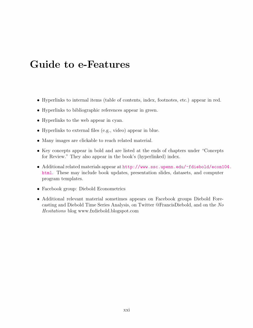
Guide to e-Features

• Hyperlinks to internal items (table of contents, index, footnotes, etc.) appear in red.

• Hyperlinks to bibliographic references appear in green.

• Hyperlinks to the web appear in cyan.

• Hyperlinks to external files (e.g., video) appear in blue.

• Many images are clickable to reach related material.

• Key concepts appear in bold and are listed at the ends of chapters under “Conceptsfor Review.” They also appear in the book’s (hyperlinked) index.

• Additional related materials appear at http://www.ssc.upenn.edu/~fdiebold/econ104.html. These may include book updates, presentation slides, datasets, and computerprogram templates.

• Facebook group: Diebold Econometrics

• Additional relevant material sometimes appears on Facebook groups Diebold Fore-casting and Diebold Time Series Analysis, on Twitter @FrancisDiebold, and on the NoHesitations blog www.fxdiebold.blogspot.com

xxi

Acknowledgments

All media (images, audio, video, ...) were either produced by me (computer graphicsusing Eviews or R, original audio and video, etc.) or obtained from the public domainrepository at Wikimedia Commons.

xxiii

xxiv Acknowledgments

List of Figures

1.1 Resources for Economists Web Page . . . . . . . . . . . . . . . . . . . . . . . 61.2 Eviews Homepage . . . . . . . . . . . . . . . . . . . . . . . . . . . . . . . . . 71.3 Stata Homepage . . . . . . . . . . . . . . . . . . . . . . . . . . . . . . . . . . 81.4 R Homepage . . . . . . . . . . . . . . . . . . . . . . . . . . . . . . . . . . . . 9

2.1 1-Year Goverment Bond Yield, Levels and Changes . . . . . . . . . . . . . . 142.2 Histogram of 1-Year Government Bond Yield . . . . . . . . . . . . . . . . . . 152.3 Bivariate Scatterplot, 1-Year and 10-Year Government Bond Yields . . . . . 162.4 Scatterplot Matrix, 1-, 10-, 20- and 30-Year Government Bond Yields . . . . 172.5 Distributions of Wages and Log Wages . . . . . . . . . . . . . . . . . . . . . 202.6 Tufte Teaching, with a First Edition Book by Galileo . . . . . . . . . . . . . 25

4.1 Distributions of Log Wage, Education and Experience . . . . . . . . . . . . . 424.2 (Log Wage, Education) Scatterplot . . . . . . . . . . . . . . . . . . . . . . . 434.3 (Log Wage, Education) Scatterplot with Superimposed Regression Line . . . 454.4 Regression Output . . . . . . . . . . . . . . . . . . . . . . . . . . . . . . . . 514.5 Wage Regression Residual Scatter . . . . . . . . . . . . . . . . . . . . . . . . 584.6 Wage Regression Residual Plot . . . . . . . . . . . . . . . . . . . . . . . . . 604.7 Carl Friedrich Gauss . . . . . . . . . . . . . . . . . . . . . . . . . . . . . . . 67

5.1 Histograms for Wage Covariates . . . . . . . . . . . . . . . . . . . . . . . . . 705.2 Wage Regression on Education and Experience . . . . . . . . . . . . . . . . . 715.3 Wage Regression on Education, Experience and Group Dummies . . . . . . . 725.4 Residual Scatter from Wage Regression on Education, Experience and Group

Dummies . . . . . . . . . . . . . . . . . . . . . . . . . . . . . . . . . . . . . 735.5 Various Linear Trends . . . . . . . . . . . . . . . . . . . . . . . . . . . . . . 745.6 Liquor Sales . . . . . . . . . . . . . . . . . . . . . . . . . . . . . . . . . . . . 785.7 Log Liquor Sales . . . . . . . . . . . . . . . . . . . . . . . . . . . . . . . . . 795.8 Linear Trend Estimation . . . . . . . . . . . . . . . . . . . . . . . . . . . . . 805.9 Residual Plot, Linear Trend Estimation . . . . . . . . . . . . . . . . . . . . . 815.10 Estimation Results, Linear Trend with Seasonal Dummies . . . . . . . . . . 825.11 Residual Plot, Linear Trend with Seasonal Dummies . . . . . . . . . . . . . 835.12 Seasonal Pattern . . . . . . . . . . . . . . . . . . . . . . . . . . . . . . . . . 845.13 Sir Ronald Fischer . . . . . . . . . . . . . . . . . . . . . . . . . . . . . . . . 86

6.1 David Hendry . . . . . . . . . . . . . . . . . . . . . . . . . . . . . . . . . . . 94

xxv

xxvi LIST OF FIGURES

7.1 Basic Linear Wage Regression . . . . . . . . . . . . . . . . . . . . . . . . . . 1017.2 Quadratic Wage Regression . . . . . . . . . . . . . . . . . . . . . . . . . . . 1027.3 Wage Regression on Education, Experience, Group Dummies, and Interactions 1037.4 Wage Regression with Continuous Non-Linearities and Interactions, and Dis-

crete Interactions . . . . . . . . . . . . . . . . . . . . . . . . . . . . . . . . . 1047.5 Various Exponential Trends . . . . . . . . . . . . . . . . . . . . . . . . . . . 1067.6 Various Quadratic Trends . . . . . . . . . . . . . . . . . . . . . . . . . . . . 1077.7 Log-Quadratic Trend Estimation . . . . . . . . . . . . . . . . . . . . . . . . 1097.8 Residual Plot, Log-Quadratic Trend Estimation . . . . . . . . . . . . . . . . 1107.9 Liquor Sales Log-Quadratic Trend Estimation with Seasonal Dummies . . . . 1117.10 Residual Plot, Liquor Sales Log-Quadratic Trend Estimation With Seasonal

Dummies . . . . . . . . . . . . . . . . . . . . . . . . . . . . . . . . . . . . . 112

9.1 Recursive Analysis, Constant Parameter Model . . . . . . . . . . . . . . . . 1309.2 Recursive Analysis, Breaking Parameter Model . . . . . . . . . . . . . . . . . 1319.3 Gregory Chow . . . . . . . . . . . . . . . . . . . . . . . . . . . . . . . . . . . 136

11.1 ***. ***. . . . . . . . . . . . . . . . . . . . . . . . . . . . . . . . . . . . . . . 17611.2 ***. ***. . . . . . . . . . . . . . . . . . . . . . . . . . . . . . . . . . . . . . . 17711.3 ***. ***. . . . . . . . . . . . . . . . . . . . . . . . . . . . . . . . . . . . . . . 17711.4 ***. ***. . . . . . . . . . . . . . . . . . . . . . . . . . . . . . . . . . . . . . . 179

12.1 Christopher Sims . . . . . . . . . . . . . . . . . . . . . . . . . . . . . . . . . 237

14.1 Time Series of Daily NYSE Returns. . . . . . . . . . . . . . . . . . . . . . . 29414.2 Correlogram of Daily Stock Market Returns. . . . . . . . . . . . . . . . . . . 29414.3 Histogram and Statistics for Daily NYSE Returns. . . . . . . . . . . . . . . . 29514.4 Time Series of Daily Squared NYSE Returns . . . . . . . . . . . . . . . . . . 29614.5 Correlogram of Daily Squared NYSE Returns. . . . . . . . . . . . . . . . . . 29614.6 GARCH(1,1) Estimation, Daily NYSE Returns. . . . . . . . . . . . . . . . . 30314.7 Estimated Conditional Standard Deviation, Daily NYSE Returns. . . . . . . 30414.8 Conditional Standard Deviation, History and Forecast, Daily NYSE Returns. 30414.9 Correlogram of Squared Standardized GARCH(1,1) Residuals, Daily NYSE

Returns. . . . . . . . . . . . . . . . . . . . . . . . . . . . . . . . . . . . . . . 30514.10AR(1) Returns with Threshold t-GARCH(1,1)-in Mean. . . . . . . . . . . . 307

15.1 Degrees-of-Freedom Penalties for Various Model Selection Criteria . . . . . . 315

List of Tables

2.1 Yield Statistics . . . . . . . . . . . . . . . . . . . . . . . . . . . . . . . . . . 22

xxvii

xxviii LIST OF TABLES

Preface

Most good texts arise from the desire to leave one’s stamp on a discipline by training

future generations of students, driven by the recognition that existing texts are deficient in

various respects. My motivation is no different, but it is more intense: In recent years I have

come to see most existing texts as highly deficient, in three ways.

First, many existing texts attempt exhaustive coverage, resulting in large tomes impos-

sible to cover in a single course (or even two, or three). Econometrics, in contrast, does not

attempt exhaustive coverage. Indeed the coverage is intentionally selective and streamlined,

focusing on the core methods with the widest applicability. Put differently, Econometrics

is not designed to impress my professor friends with the breadth of my knowledge; rather,

it’s designed to teach real students and can be realistically covered in a one-semester course.

Core material appears in the main text, and additional material appears in the end-of-chapter

“Exercises, Problems and Complements,” as well as the Bibliographical and Computational

Notes.

Second, many existing texts emphasize theory at the expense of serious applications.

Econometrics, in contrast, is applications-oriented throughout, using detailed real-world ap-

plications not simply to illustrate theory, but to teach it (in truly realistic situations in

which not everything works perfectly!). Econometrics uses modern software throughout (R,

Eviews and Stata), but the discussion is not wed to any particular software – students and

instructors can use whatever computing environment they like best.

Third, almost all existing texts remain shackled by Middle-Ages paper technology. Econo-

metrics, in contrast, is e-aware. It’s colorful, hyperlinked internally and externally, and tied

to a variety of media – effectively a blend of a traditional “book”, a DVD, a web page, a

Facebook group, a blog, and whatever else I can find that’s useful. It’s continually evolving

and improving on the web, and its price is much closer to $20 than to the obscene but now-

standard $200 for a pile of paper. It won’t make me any new friends among the traditional

publishers, but that’s not my goal.

Econometrics should be useful to students in a variety of fields – in economics, of course,

xxix

xxx PREFACE

but also business, finance, public policy, statistics, and even engineering. It is directly acces-

sible at the undergraduate and master’s levels, and the only prerequisite is an introductory

probability and statistics course. I have used the material successfully for many years in my

undergraduate econometrics course at Penn, as background for various other undergraduate

courses, and in master’s-level executive education courses given to professionals in economics,

business, finance and government.

Many people have contributed to the development of this book – some explicitly, some

without knowing it. One way or another, all of the following deserve thanks:

• Frank Di Traglia, University of Pennsylvania

• Damodar Gujarati, U.S. Naval Academy

• James H. Stock, Harvard University

• Mark W. Watson, Princeton University

I am especially grateful to an army of energetic and enthusiastic Penn undergraduate

and graduate students, who read and improved much of the manuscript, and to Penn itself,

which for many years has provided an unparalleled intellectual home, the perfect incubator

for the ideas that have congealed here. Special thanks go to

• Li Mai

• John Ro

• Carlos Rodriguez

• Zach Winston

Finally, I apologize and accept full responsibility for the many errors and shortcomings

that undoubtedly remain – minor and major – despite ongoing efforts to eliminate them.

Francis X. Diebold

Philadelphia

Tuesday 4th February, 2014

Econometrics

Part I

Preliminaries

1

Chapter 1

Introduction to Econometrics

1.1 Welcome

1.1.1 Who Uses Econometrics?

Econometric modeling is important — it is used constantly in business, finance, eco-

nomics, government, consulting and many other fields. Econometric models are used rou-

tinely for tasks ranging from data description to and policy analysis, and ultimately they

guide many important decisions.

To develop a feel for the tremendous diversity of econometrics applications, let’s sketch

some of the areas where it features prominently, and the corresponding diversity of decisions

supported.

One key field is economics (of course), broadly defined. Governments, businesses, policy

organizations, central banks, financial services firms, and economic consulting firms around

the world routinely use econometrics.

Governments use econometric models to guide monetary and fiscal policy.

Another key area is business and all its subfields. Private firms use econometrics for

strategic planning tasks. These include management strategy of all types including oper-

ations management and control (hiring, production, inventory, investment, ...), marketing

(pricing, distributing, advertising, ...), accounting (budgeting revenues and expenditures),

and so on.

Sales modeling is a good example. Firms routinely use econometric models of sales to help

guide management decisions in inventory management, sales force management, production

planning, new market entry, and so on.

More generally, firms use econometric models to help decide what to produce (What

product or mix of products should be produced?), when to produce (Should we build up

3

4 CHAPTER 1. INTRODUCTION TO ECONOMETRICS

inventories now in anticipation of high future demand? How many shifts should be run?),

how much to produce and how much capacity to build (What are the trends in market size

and market share? Are there cyclical or seasonal effects? How quickly and with what pattern

will a newly-built plant or a newly-installed technology depreciate?), and where to produce

(Should we have one plant or many? If many, where should we locate them?). Firms also

use forecasts of future prices and availability of inputs to guide production decisions.

Econometric models are also crucial in financial services, including asset management,

asset pricing, mergers and acquisitions, investment banking, and insurance. Portfolio man-

agers, for example, have been interested in empirical modeling and understanding of asset

returns such as stock returns, interest rates, exchange rates, and commodity prices.

Econometrics is similarly central to financial risk management. In recent decades, eco-

noemtric methods for volatility modeling have been developed and widely applied to evaluate

and insure risks associated with asset portfolios, and to price assets such as options and other

derivatives.

Finally, econometrics is central to the work of a wide variety of consulting firms, many

of which support the business functions already mentioned. Litigation support is also a very

active area, in which econometric models are routinely used for damage assessment (e.g.,

lost earnings), “but for” analyses, and so on.

Indeed these examples are just the tip of the iceberg. Surely you can think of many more

situations in which econometrics is used.

1.1.2 What Distinguishes Econometrics?

Econometrics is much more than just “statistics using economic data,” although it is of

course very closely related to statistics.

– Econometrics must confront the fact that economic data is not generated from well-

designed experiments. On the contrary, econometricians must generally take whatever so-

called “observational data” they’re given.

– Econometrics must confront the special issues and features that arise routinely in

economic data, such as trends and cycles.

– Econometricians are sometimes interested in predictive modeling, which requires under-

standing only correlations, and sometimes interested in evaluating treatment effects, which

involve deeper issues of causation.

With so many applications and issues in econometrics, you might fear that a huge variety

of econometric techniques exists, and that you’ll have to master all of them. Fortunately,

that’s not the case. Instead, a relatively small number of tools form the common core of

much econometric modeling. We will focus on those underlying core principles.

1.2. TYPES OF RECORDED ECONOMIC DATA 5

1.2 Types of Recorded Economic Data

Several aspects of economic data will concern us frequently.

One issue is whether the data are continuous or binary. Continuous data take values

on a continuum, as for example with GDP growth, which in principle can take any value in

the real numbers. Binary data, in contrast, takes just two values, as with a 0-1 indicator

for whether or not someone purchased a particular product during the last month.

Another issue is whether the data are recorded over time, over space, or some combination

of the two. Time series data are recorded over time, as for example with U.S. GDP, which

is measured once per quarter. A GDP dataset might contain data for, say, 1960.I to the

present. Cross sectional data, in contrast, are recorded over space (at a point in time), as

with yesterday’s closing stock price for each of the U.S. S&P 500 firms. The data structures

can be blended, as for example with a time series of cross sections. If, moreover, the

cross-sectional units are identical over time, we speak of panel data.1 An example would

be the daily closing stock price for each of the U.S. S&P 500 firms, recorded over each of the

last 30 days.

1.3 Online Information and Data

Much useful information is available on the web. The best way to learn about what’s out

there is to spend a few hours searching the web for whatever interests you. Here we mention

just a few key “must-know” sites. Resources for Economists, maintained by the American

Economic Association, is a fine portal to almost anything of interest to economists. (See

Figure 1.1.) It contains hundreds of links to data sources, journals, professional organizations,

and so on. FRED (Federal Reserve Economic Data) is a tremendously convenient source for

economic data. The National Bureau of Economic Research site has data on U.S. business

cycles, and the Real-Time Data Research Center at the Federal Reserve Bank of Philadelphia

has real-time vintage macroeconomic data. Finally, check out Quandl, which provides access

to millions of data series on the web.

1.4 Software

Econometric software tools are widely available. One of the best high-level environments

is Eviews, a modern object-oriented environment with extensive time series, modeling and

forecasting capabilities. (See Figure 1.2.) It implements almost all of the methods described

1Panel data is also sometimes called longitudinal data.

6 CHAPTER 1. INTRODUCTION TO ECONOMETRICS

Figure 1.1: Resources for Economists Web Page

in this book, and many more. Eviews reflects a balance of generality and specialization that

makes it ideal for the sorts of tasks that will concern us, and most of the examples in this

book are done using it. If you feel more comfortable with another package, however, that’s

fine – none of our discussion is wed to Eviews in any way, and most of our techniques can

be implemented in a variety of packages.

Eviews has particular strength in time series environments. Stata is a similarly good

packaged with particular strength in cross sections and panels. (See Figure 1.3.)

Eviews and Stata are examples of very high-level modeling environments. If you go on to

more advanced econometrics, you’ll probably want also to have available slightly lower-level

(“mid-level”) environments in which you can quickly program, evaluate and apply new tools

and techniques. R is one very powerful and popular such environment, with special strengths

in modern statistical methods and graphical data analysis. (See Figure 1.4.) In this author’s

humble opinion, R is the key mid-level econometric environment for the foreseeable future.

1.5. TIPS ON HOW TO USE THIS BOOK 7

Figure 1.2: Eviews Homepage

1.5 Tips on How to use this book

As you navigate through the book, keep the following in mind.

• Hyperlinks to internal items (table of contents, index, footnotes, etc.) appear in red.

• Hyperlinks to references appear in green.

• Hyperlinks to external items (web pages, video, etc.) appear in cyan.2

• Key concepts appear in bold and are listed at the ends of chapters under “Concepts

for Review.” They also appear in the (hyperlinked) index.

• Many figures are clickable to reach related material, as are, for example, all figures in

this chapter.

• Most chapters contain at least one extensive empirical example in the “Econometrics

in Action” section.

2Obviously web links sometimes go dead. I make every effort to keep them updated in the latest edition(but no guarantees of course!). If you’re encountering an unusual number of dead links, you’re probablyusing an outdated edition.

8 CHAPTER 1. INTRODUCTION TO ECONOMETRICS

Figure 1.3: Stata Homepage

• The end-of-chapter “Exercises, Problems and Complements” sections are of central

importance and should be studied carefully. Exercises are generally straightforward

checks of your understanding. Problems, in contrast, are generally significantly more

involved, whether analytically or computationally. Complements generally introduce

important auxiliary material not covered in the main text.

1.6 Exercises, Problems and Complements

1. (No example is definitive!)

Recall that, as mentioned in the text, most chapters contain at least one extensive

empirical example in the “Econometrics in Action” section. At the same time, those

examples should not be taken as definitive or complete treatments – there is no such

thing! A good idea is to think of the implicit “Problem 0” at the end of each chapter

as “Critique the modeling in this chapter’s Econometrics in Action section, obtain the

relevant data, and produce a superior analysis.”

2. (Nominal, ordinal, interval and ratio data)

1.6. EXERCISES, PROBLEMS AND COMPLEMENTS 9

Figure 1.4: R Homepage

We emphasized time series, cross-section and panel data, whether continuous or dis-

crete, but there are other complementary categorizations. In particular, distinctions

are often made among nominal data, ordinal data, interval data, and ratio data.

Which are most common and useful in economics and related fields, and why?

3. (Software at your institution)]

Which of Eviews and Stata are installed at your institution? Where, precisely, are

they? How much would it cost to buy them?

4. (Software differences and bugs: caveat emptor)

Be warned: no software is perfect. In fact, all software is highly imperfect! The results

obtained when modeling in different software environments may differ – sometimes a

little and sometimes a lot – for a variety of reasons. The details of implementation may

differ across packages, for example, and small differences in details can sometimes pro-

duce large differences in results. Hence, it is important that you understand precisely

what your software is doing (insofar as possible, as some software documentation is

10 CHAPTER 1. INTRODUCTION TO ECONOMETRICS

more complete than others). And of course, quite apart from correctly-implemented

differences in details, deficient implementations can and do occur: there is no such

thing as bug-free software.

1.7 Historical and Computational Notes

For a compendium of econometric and statistical software, see the software links site, main-

tained by Marius Ooms at the Econometrics Journal.

R is available for free as part of a massive and highly-successful open-source project. R-

bloggers is a massive blog with all sorts of information about all things R. RStudio provides

a fine R working environment, and, like R, it’s free. Finally, Quandl has a nice R interface.

1.8. PRODUCERS AND USERS OF ECONOMETRICS, OLD AND NEW 11

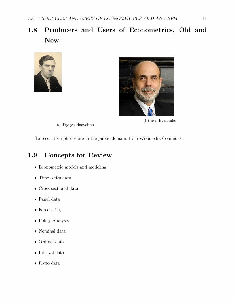
1.8 Producers and Users of Econometrics, Old and

New

(a) Trygve Haavelmo(b) Ben Bernanke

Sources: Both photos are in the public domain, from Wikimedia Commons.

1.9 Concepts for Review

• Econometric models and modeling

• Time series data

• Cross sectional data

• Panel data

• Forecasting

• Policy Analysis

• Nominal data

• Ordinal data

• Interval data

• Ratio data

12 CHAPTER 1. INTRODUCTION TO ECONOMETRICS

Chapter 2

Graphical Analysis of Economic Data

It’s almost always a good idea to begin an econometric analysis with graphical data analysis.

When compared to the modern array of econometric methods, graphical analysis might seem

trivially simple, perhaps even so simple as to be incapable of delivering serious insights.

Such is not the case: in many respects the human eye is a far more sophisticated tool for

data analysis and modeling than even the most sophisticated statistical techniques. Put

differently, graphics is a sophisticated technique. That’s certainly not to say that graphical

analysis alone will get the job done – certainly, graphical analysis has its limitations of its

own – but it’s usually the best place to start. With that in mind, we introduce in this chapter

some simple graphical techniques, and we consider some basic elements of graphical style.

2.1 Simple Techniques of Graphical Analysis

We will segment our discussion into two parts: univariate (one variable) and multivariate

(more than one variable). Because graphical analysis “lets the data speak for themselves,”

it is most useful when the dimensionality of the data is low; that is, when dealing with

univariate or low-dimensional multivariate data.

2.1.1 Univariate Graphics

First consider time series data. Graphics is used to reveal patterns in time series data. The

great workhorse of univariate time series graphics is the simple time series plot, in which

the series of interest is graphed against time.

In the top panel of Figure 2.1, for example, we present a time series plot of a 1-year

Government bond yield over approximately 500 months. A number of important features of

the series are apparent. Among other things, its movements appear sluggish and persistent,

13