econometrics: problem sets - academia madrid … noteboo… · econometrics: problem sets 1 ......
TRANSCRIPT

ECONOMETRICS: Problem Sets
1
ECONOMETRICS
: Problem Sets
ACADEMIC YEAR: 2017-2018 CAMPUS: Segovia - Madrid Professors: Rodrigo Alegría & Ainara González de San Román

ECONOMETRICS: Problem Sets
2
PREFACE
This document contains exercises for you to practice with the content of the course in a
practical way. Some of them will be included in the so-called Problem Sets, which will be
solved in class. Students are required to work by themselves on these Problem Sets. Exercises
to be solved within each Problem Set will be announced in advance to the due date. We will
solve five Problem Sets during the course.
Important: All rights reserved. No part of this document may be reproduced, in any form
or by any means, without the permission in writing from the author.
Any errors in this document are the responsibility of the author. Corrections and comments
regarding any material in this text are welcomed and appreciated.
Authors: Rodrigo Alegría & Ainara González de San Román
e-mail: [email protected] & [email protected]

ECONOMETRICS: Problem Sets
3
CONTENTS
Problem Set 1: Descriptive and
Correlation Analysis.
Problem Set 2: Linear Regression
Analysis.
Problem Set 3: Hypothesis
Testing.
Problem Set 4: Qualitative
Analysis (dummy variables).
...................................... 4
...................................... 13
...................................... 36
...................................... 53
Problem Set 5: Estimation Problems ...................................... 73
and Time Series

ECONOMETRICS: Problem Sets
4
PS1
Descriptive and Correlation
Analysis
COURSE CONTENT
-Chapter 1: Introduction, Data and Econometric Modelling.
-Chapter 2: Review of Statistics, Descriptive Analysis and
Correlation Analysis.
-Chapter 3: Estimator and its properties.
I asked an econometrician for her phone number…
and she gave me an estimate.

ECONOMETRICS: Problem Sets
5
1 Determine the type of data of the following variables:
a- Italian monthly salaries in the time period 1980-2005.
b- Gender distribution in each of the OECD countries in 2010.
c- Inflation rate in each of the OECD countries in 2008.
d- R&D expenditure in each of the European Union member states in 2003.
e- Yearly automobile production in France, Italy and Spain in the time period 1980-
2010.
f- Yearly race distribution in the United States during the last 20 years.
g- Monthly water consumption during the 20th century in the city of Madrid.
2 Suppose you are asked to conduct a study to determine whether small class sizes
lead to increase student performance.
a- Postulate an econometric model that allows you to conduct this study.
b- Why might you expect a negative correlation between class size and student
performance?
c- Would a negative correlation necessarily show that smaller class sizes cause better
performance? Explain.
3 A substitute teacher wants to know how students in the class did on their last test.
The teacher asks the 10 students sitting in the front row to state their latest test score. He
concludes from their report that the class did extremely well.
a- What is the sample? What is the population?
b- Could you identify any problems with choosing the sample in this way?
4 Suppose that X is the number of free throws make by a basketball player out of two
attempts and assume that the individual probabilities for each outcome of X are the
following: pr(x=0)=0.2; pr(x=1)=0.44 and pr(x=2)=0.36
a- Define the random variable.
b- Draw the probability distribution associated to the above random variable.
c- Calculate the expected value of the above random variable.
d- Calculate the probability that the player makes at least one free throw.

ECONOMETRICS: Problem Sets
6
5 Interpret the following graphs in terms of association, correlation and relationship:
6 Suppose 𝑥1 and 𝑥2 are independent random variables with means 𝜇1, 𝜇2 and
standard deviations 𝜎1 and 𝜎2.
a- Find the mean and variance for a new random variable 𝑢 = 𝑥1 − 𝑏𝑥2
b- Find the mean and variance for a new random variable 𝑣 = 𝑎𝑥2 + 𝑏𝑥1
7 The table below shows data about annual salaries (thousand Euros) and tenure (years)
for 8 individual working in a company:
Salary 40 22 19 30 62 32 45 51
Tenure 15 3 1 8 39 13 17 24
a- What is your expectation about the type of relationship that exist between the two
variables?
b- Compute the linear correlation coefficient between salaries and tenure and interpret
your result.
c- Which variable is more dispersed? Why?

ECONOMETRICS: Problem Sets
7
8 In the table below, E denotes the employment growth rate and P the productivity
growth rate in the manufacturing industry in six countries for the period 1980-1990.
Country E P
Austria 2.0 4.0
Belgium 1.7 3.9
Canada 2.0 1.5
Denmark 2.4 3.0
Italy 4.0 2.0
Japan 5.9 9.6
a- Determine whether the data is a time series, a cross sectional data or panel data.
b- Draw a scatter plot with the data of the table. Interpret your graph.
c- Calculate the correlation coefficient (E, P) and interpret your result.
d- Calculate a new correlation coefficient eliminating the Japanese observation and
interpret your result.
9 Let 𝑋 be a random variable knowing that:
𝐸(𝑥) = 𝜇 = 1 𝑎𝑛𝑑 𝑉𝑎𝑟(𝑥) = 𝜎2 = 1
We have information about four independent observations: 𝑥1, 𝑥2, 𝑥3, 𝑥4.
a- Let ��1 y ��2 be two different estimators of 𝜇, find which one is more appropriate
according to the mean square error (MSE).
��1 =𝑥1 + 𝑥2 + 𝑥3
3 ; ��2 =
𝑥1 + 𝑥4
6
b- Discuss the sufficiency of both estimators.
c- Suggest a sufficient estimator of 𝜇 and with a MSE lower than the above ones.
10 We define a random variable 𝑋 as tossing three coins. If we define the experiment as
the number of tails obtained:
a- Define the random variable.
b- Find the probability distribution for X.
c- Calculate 𝐸(𝑋).

ECONOMETRICS: Problem Sets
8
11 In the table below, P denotes average property prices and S average property sizes in
six cities in 2012.
Country P S
New York 10.2 6.7
Madrid 7.2 5.5
Rome 9.0 5.8
London 11.6 7.7
Paris 10.8 7.1
Tokyo 17.2 3.1
a- Determine whether the data is a time series, a cross sectional data or panel data.
b- Draw a scatter plot with the data of the table. Interpret your graph.
c- Find the correlation coefficient (P, S) and interpret your result.
d- Find a new correlation coefficient eliminating the Tokyo observation and interpret
your result.
12 Let 𝑋 be a random variable knowing that:
𝐸(𝑥) = 𝜇 𝑎𝑛𝑑 𝑉𝑎𝑟(𝑥) = 𝜎2
We have information about four independent observations: 𝑥1, 𝑥2, 𝑥3, 𝑥4.
Let ��1 = 1
4(𝑥1 + 𝑥2 + 𝑥3 + 𝑥4) being and estimator for the population mean.
a- What are the expected value and variance of ��1 in terms of 𝜇 and 𝜎2?
b- Now consider a second estimator for the population mean ��2 being defined as:
��2 =1
8𝑥1 +
1
8𝑥2 +
1
4𝑥3 +
1
2𝑥4
Show that this second estimator is also an unbiased estimator for the population
mean. Find its variance.
c- Discuss the sufficiency of both estimators.
d- Based on all your previous answers, which estimator do you prefer?

ECONOMETRICS: Problem Sets
9
13 We define a random variable 𝑥 as the resulting sum when tossing two dices. .
a- Find the probability distribution for 𝑥
b- Compute the 𝐸(𝑥)
c- Calculate 𝐸(𝑦) knowing that 𝑦 = 2𝑥 − 1.
14 Evaluate in which of the below cases you can say that the presented results are
compatible and explain why:
a- 𝐶𝑜𝑣(𝑥, 𝑦) = 25.33 and 𝜌 = −0.37
b- 𝑠𝑥2 = 1,000 𝑛 = 50 ∑ 𝑥𝑖
𝑛𝑖=1 = 5,000 and 𝐶𝑉(𝑥) = 0.316
c-
and 𝜌 = 0.775
15 In the table below, U denotes the unemployment rate and I the inflation rate in six
American countries in 2011.
Country U I
Mexico 5.2 3.4
Argentina 7.2 9.5
Brazil 6.0 6.6
Chile 6.6 3.3
Colombia 10.8 3.4
Venezuela 8.2 26.1
a- Determine whether the data is a time series, a cross sectional data or panel data.
b- Draw a scatter plot with the data of the table. Interpret your graph.
c- Calculate the correlation coefficient (U, I) and interpret your result.
d- Calculate a new correlation coefficient eliminating the Venezuelan observation and
interpret your result.

ECONOMETRICS: Problem Sets
10
16 Let 𝑋 be a random variable knowing that:
𝐸(𝑥) = 𝜇 = 1 𝑎𝑛𝑑 𝑉𝑎𝑟(𝑥) = 𝜎2 = 1
We have information about four observations: 𝑥1, 𝑥2, 𝑥3, 𝑥4.
a- Let ��1 y ��2 be two different estimators of 𝜇, find which one is more appropriate
according to the mean square error (MSE).
��1 =𝑥1 + 𝑥2
2 ; ��2 =
𝑥1 + 𝑥4
4
Note: Observations are independent.
b- Discuss the sufficiency of both estimators.
c- Suggest a sufficient estimator of 𝜇 and with a MSE lower than the above ones.
17 A professor teaches a large class and has scheduled an exam for 7:00 pm in a different
classroom. She estimates the probabilities in the table for the number of students who will call her
at home in the hour before the exam asking where the exam will be held.
a- Draw the probability distribution associated to the above experiment.
b- Find the expected value of the number of calls.
18 A specific company has observed in the last 5 months that their sales depend on the
amount invested in advertising. Observe the table below:
Advertising Expenses Sales
$ 100,000 R$ 1,000,000
$ 200,000 R$ 1,000,000
$ 300,000 R$ 2,000,000
$ 400,000 R$ 2,000,000
$ 500,000 R$ 4,000,000

ECONOMETRICS: Problem Sets
11
a- Construct a scatter plot of the data. Does a clear linear relationship exist between the two variables?
b- Conduct a descriptive and correlation analysis of the above data and interpret both analysis.
19 In this exercise a researcher uses data on NBA players’ salaries and their
determinants. She is interested in knowing the effect of performance on NBA players’
salaries. The following information is available for 56 NBA players.
Table 1. Variables of the dataset – names and description
SALARY = Salary earned by players in thousands of dollars. HT = Height of the players in inches. WT = Weight of each player in pounds. AGE = Age of each player MIN = Number of minutes that each player played during the season. STEALS = Number of times that player stole ball from opponents. BLOCKS = Number of blocked shots. POINTS = Number of points that the player scored in the full season.
The summary statistics for all the variables in Table 1, as well as the correlation matrix, are
presented in Tables 2 and 3 respectively.
Table 2. Summary statistics
Variable Mean Std. Dev. Minimum Maximum SALARY 1668.04 667.910 1000 3750
HT 80.6250 3.66091 73 88 WT 226.804 26.7034 175 290
AGE 28.4107 3.03181 23 36 MIN 2538.96 670.669 189 3255
STEALS 97.9821 85.9193 6 564 BLOCKS 70.5179 74.0361 5 315 POINTS 1369.68 578.186 116 2633
Table 3. Correlation matrix
SALARY HT WT AGE MIN STEALS BLOCKS POINTS
SALARY 1 0.003 0.048 -0.075 0.094 0.082 0.088 0.233
HT 1 0.832 0.2926 -0.345 -0.349 0.556 -0.365
WT 1 0.086 -0.184 -0.225 0.473 -0.289
AGE 1 -0.112 -0.346 0.169 -0.081
MIN 1 0.319 0.048 0.793
STEALS 1 -0.128 0.386
BLOCKS 1 -0.078
POINTS 1

ECONOMETRICS: Problem Sets
12
Answer the following questions:
a- Is this a cross-section or a time series? Why? Which is the unit of analysis in this data
set? And the sample size?
b- How old is the youngest basketball player of this sample?
c- Could you tell which variable is more dispersed by looking at the values of the
standard deviations in Table 2?
d- Could you say, by looking at Table 3, that there is a penalty in terms of lower wages
associated with age? Explain.
e- Which variables have the highest correlation (positive or negative) with wage?
Explain.
20 Let Y1, Y2, Y3, and Y4 be independent, identically distributed random variables from
a population with mean μ and variance σ2. Let Y be:
𝑌 =1
4𝑌1 +
1
6𝑌2 +
1
2𝑌3 +
1
4𝑌4
denoting the average of these four random variables. Show that Y is a biased estimator of μ.

ECONOMETRICS: Problem Sets
13
PS2
Linear Regression
Analysis
COURSE CONTENT
-Chapter 4: Linear Regression Analysis
-Simple Linear Regression Model.
-Multiple Linear Regression Model.
An econometrician was asked about the meaning of life. He replied: It depends on the parameter values.
ECONOMETRICS: Problem Sets
14
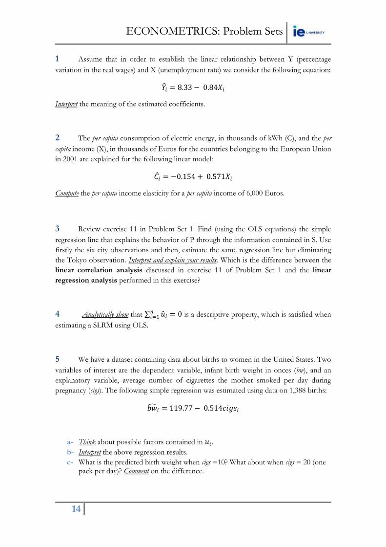
1 Assume that in order to establish the linear relationship between Y (percentage
variation in the real wages) and X (unemployment rate) we consider the following equation:
��𝑖 = 8.33 − 0.84𝑋𝑖
Interpret the meaning of the estimated coefficients.
2 The per capita consumption of electric energy, in thousands of kWh (C), and the per
capita income (X), in thousands of Euros for the countries belonging to the European Union
in 2001 are explained for the following linear model:
��𝑖 = −0.154 + 0.571𝑋𝑖
Compute the per capita income elasticity for a per capita income of 6,000 Euros.
3 Review exercise 11 in Problem Set 1. Find (using the OLS equations) the simple
regression line that explains the behavior of P through the information contained in S. Use
firstly the six city observations and then, estimate the same regression line but eliminating
the Tokyo observation. Interpret and explain your results. Which is the difference between the
linear correlation analysis discussed in exercise 11 of Problem Set 1 and the linear
regression analysis performed in this exercise?
4 Analytically show that ∑ ��𝑖𝑛𝑖=1 = 0 is a descriptive property, which is satisfied when
estimating a SLRM using OLS.
5 We have a dataset containing data about births to women in the United States. Two
variables of interest are the dependent variable, infant birth weight in onces (bw), and an
explanatory variable, average number of cigarettes the mother smoked per day during
pregnancy (cigs). The following simple regression was estimated using data on 1,388 births:
𝑏��𝑖 = 119.77 − 0.514𝑐𝑖𝑔𝑠𝑖
a- Think about possible factors contained in 𝑢𝑖 .
b- Interpret the above regression results.
c- What is the predicted birth weight when cigs =10? What about when cigs = 20 (one pack per day)? Comment on the difference.

ECONOMETRICS: Problem Sets
15
6 A company A operates with the following production function:
𝑌𝑡𝐴 = 110 + 0.65𝐾𝑡
𝐴 (𝑅𝐴2 = 0.37)
Such that 𝑌𝑡𝐴 measures total production in thousand Euros in year 𝑡 and 𝐾𝑡
𝐴 measures the
use of capital in thousand Euros in year 𝑡.
a- Interpret the coefficients of the estimated production function.
b- A competitor of company A, company B, operates according to a different
production function defined as:
𝑌𝑡𝐵 = 80 + 0.50𝐾𝑡
𝐵 (𝑅𝐵2 = 0.48)
Interpret the coefficients of the estimated production function for company B in
comparison to the coefficients for company A.
c- In 2010 (𝑡 = 2010), the use of capital in company A had a value of 320,000 Euros
and 280,000 Euros in company B. Both companies are planning to expand their
businesses to the Brazilian market in 2015. Therefore, their capital levels will increase
20% respect to 2010. Find the total production prediction in 2015 (𝑡 = 2015) for
each company using the estimated cost functions. Explain which company will obtain
a more accurate prediction in your opinion.
d- Do you think the relationship between production and the use of capital has constant
returns (whether linearity assumption is satisfied)? If no, specify a more realistic
regression model.
7 Are rent rates influenced by the city population? Using 2005 data for 70 cities, the
following equation relates rent rates (rent) to total city population (pop):
log(𝑟𝑒𝑛��) = 9.40 + 0.0312 log(𝑝𝑜𝑝) 𝑅2 = 0.192 𝑛 = 70
a- Interpret the coefficient on log(pop). Is the sign of this estimate what you expect it to be?
b- Interpret the determination coefficient. Why do you think is such a low value?
c- What other factors about a property may affect its rental price?

ECONOMETRICS: Problem Sets
16
8 We have the following information regarding the average growth rates of
employment (e) and real GDP (g) for 25 OECD countries for the period 1988-2007:
�� = 0.83 �� = 2.82 𝑆𝑆𝑇 = 14.57 𝑆𝑆𝑅 = 6.12
∑(𝑒𝑖 − ��)(𝑔𝑖 − ��) = 29.76 ∑(𝑔𝑖 − ��)2 = 60.77
25
𝑖=1
25
𝑖=1
a- Find the regression coefficients for a regression model that investigates the behaviour
of e through the behaviour of g.
b- Interpret your regression coefficients.
c- Find and interpret the value of the determination coefficient.
d- Calculate the predicted e when g=3.15.
9 Review exercise 8 in Problem Set 1. Find (using the OLS equations) the simple
regression line that explains the behavior of E through the information contained in P. Use
firstly the six country observations and then, estimate the same regression line but eliminating
the Japanese observation. Interpret and explain your results. Which is the difference between the
linear correlation analysis discussed in exercise 8 of Problem Set 1 and the linear
regression analysis performed in this exercise?
10 Analytically show that if you estimate a SLRM using OLS method of estimation the
𝐶𝑜𝑣(𝑦��, ��𝑖) = 0
11 The CAMP (Capital Asset Pricing Model) is an equilibrium model explaining the
expected returns for assets. The regression for the excess of return (over the free-risk asset)
has the following econometric specification:
(𝑅𝑡 − 𝑟𝑡𝑓
) = 𝛽0 + 𝛽1(𝑅𝑡𝑀 − 𝑟𝑡
𝑓) + 𝑢𝑡
Where, for the 𝑡 − 𝑡ℎ month, 𝑅𝑡 represents the return of the asset, 𝑟𝑡𝑓is the monthly return
of the risk-free asset (for example, the Treasury bills with a maturity of 30 days), 𝑅𝑡𝑀 is the

ECONOMETRICS: Problem Sets
17
return of the market available assets, and 𝑢𝑡 is the random perturbance term that captures
the random fluctuations that are independent on the market portfolio.
a- Interpret 𝛽1.
b- What can be say about an asset with 𝛽1 = 1? And one with 𝛽1 > 1? And with
𝛽1 < 1?
c- Explain the G-M condition that is being described above.
12 Review exercise 18 in Problem Set 1.
a- Estimate the Simple Linear Regression Model associated to the data. Interpret
your estimation results.
b- If the company invests 355,000 in advertising, what is the forecasted amount of
sales?
13 Observe the table below:
X Y
62 8.1
70 9.0
76 9.2
82 10.5
88 10.8
74 9
75 8.1
a- Estimate the relationship between X and Y using OLS; that is obtain the intercept and
slope estimates in the regression equation.
b- Compute the fitted values and residuals for each observation, and verify if residuals
(approximately) sum to zero.
c- What is the predicted value of Y when X=58?
d- How much of the variation in Y for these 7 observations is explained by X?

ECONOMETRICS: Problem Sets
18
14 The following data give X, the price charged per piece of playwood, and Y, the quantity
sold (in thousands).
Price per Piece Thousands of Pieces Sold
$6 80
$7 60
$8 70
$9 40
$10 0
a- Draw a scatter plot and interpret it.
b- Compute SST, SSR and SSE and explain the difference between SSE and SSR.
c- Compute the coefficient of determination and the value of the sample correlation coefficient. Explain the difference between them.
15 A company A operates with the following production function:
𝑌𝑡𝐴 = 120 + 0.75𝐿𝑡
𝐴 (𝑅𝐴2 = 0.38)
Such that 𝑌𝑡𝐴 measures total production in thousand Euros in year 𝑡 and 𝐿𝑡
𝐴 measures the
use of labour in number of workers in year 𝑡.
a- Interpret the coefficients of the estimated production function.
b- A competitor of company A, company B, operates according to a different
production function defined as:
𝑌𝑡𝐵 = 70 + 0.45𝐿𝑡
𝐵 (𝑅𝐴2 = 0.58)
Interpret the coefficients of the estimated production function for company B in
comparison to the coefficients for company A.
c- In 2010 (𝑡 = 2010), the use of labour in company A had a value of 3,500 workers
and 2,800 workers in company B. Both companies are planning to expand their
businesses to the Chinese market in 2015. Therefore, their labor levels will increase
20% respect to 2010. Find the total production prediction in 2015 (𝑡 = 2015) for
each company using the estimated production functions. Explain which company will
obtain a more accurate prediction in your opinion.

ECONOMETRICS: Problem Sets
19
d- Do you think the relationship between production and the use of labor has constant
returns (whether linearity assumption is satisfied)? If no, specify a more realistic
regression model.
16 Analytically show that the OLS estimator for the intercept in a Simple Linear Regression
Model is an unbiased estimator.
17 We denote 𝐼𝑖 as total investment in a country (million dollars) and 𝐼𝑅𝑖 represents the
interest rate. We consider the following linear regression model that yields the relationship
between I and IR:
𝐼𝑖 = 𝛽0 + 𝛽1𝐼𝑅𝑖 + 𝑢𝑖
such that 𝑢𝑖 denotes an unobservable error (random perturbances).
d- Think about possible factors contained in 𝑢𝑖 .
e- Knowing that 𝐼 = 0.25, 𝐼𝑅 = 5, Cov(I, IR)=-0.7 and Var(IR)=0.45, find the
estimated value for the intercept and slope coefficients and interpret your results.
f- Could you specify and explain a theoretical regression model of the above relationship
in order to take into account decreasing returns in the effect of 𝐼𝑅𝑖on 𝐼𝑖?
18 A company A operates with the following cost function:
𝑇𝐶𝑡𝐴 = 220 + 0.45𝑃𝑡
𝐴 (𝑅𝐴2 = 0.57)
Such that 𝑇𝐶𝑡𝐴 measures total production costs in thousand Euros in year 𝑡 and 𝑃𝑡
𝐴 measures
the level of production in thousand Euros in year 𝑡.
a- Interpret the coefficients of the estimated cost function.
b- A competitor of company A, company B, operates according to a different cost
function defined as:
𝑇𝐶𝑡𝐵 = 280 + 0.38𝑃𝑡
𝐵 (𝑅𝐵2 = 0.42)
Interpret the coefficients of the estimated cost function for company B in comparison
to the coefficients for company A.

ECONOMETRICS: Problem Sets
20
c- In 2010 (𝑡 = 2010), the level of production in company A had a value of 430,000
Euros and 380,000 Euros in company B. Both companies are planning to expand
their businesses to the Indian market in 2015. Therefore, their production levels will
increase 20% respect to 2010. Find the total costs prediction in 2015 (𝑡 = 2015) for
each company using the estimated cost functions. Explain which company will obtain
a more accurate prediction in your opinion.
19 A political party is investigating whether spending in marketing (𝑚𝑒𝑡), measured in
thousand Euros, is an appropriate strategy in order to gain more members in the parliament
(𝑀𝑡) for the next elections:
𝑀𝑡 = 𝛽0 + 𝛽1𝑚𝑒𝑡 + 𝑢𝑡
In order to estimate the above regression model, data of the last five elections is collected
obtaining the following estimated regression:
𝑀�� = 2.684 + 0.025𝑚𝑒𝑡 𝑇 = 5 𝑅2 = 0.392
e- Interpret the constant term.
f- Interpret ��1 (slope-estimated coefficient).
g- Interpret the value of the determination coefficient.
h- Find the predicted members in the parliament if the political party is thinking in
spending about 750,000 Euros in marketing for the next elections.
20 Review exercise 15 in Problem Set 1. Find (using the OLS equations) the
simple regression line that explains the behavior of I through the information contained in
U. Use firstly the six country observations and then, estimate the same regression line but
eliminating the Venezuelan observation. Interpret and explain your results. Which is the
difference between the linear correlation analysis discussed in exercise 15 of Problem Set
1 and the linear regression analysis performed in this exercise?

ECONOMETRICS: Problem Sets
21
21 A production function for a company is estimated using yearly observations for 20
years and we obtain the following estimated regression model:
𝑙𝑜𝑔 (𝑝𝑟𝑜𝑑𝑢𝑐𝑡𝑖𝑜𝑛)𝑡 = 4.822 + 0.257 log(𝑐𝑎𝑝𝑖𝑡𝑎𝑙)𝑡 𝑅2 = 0.311 𝑇 = 20
Where both production and the use of capital are measured in thousand Euros.
a- Interpret the the coefficient on log(capital). Is the sign of this estimate what you expect it to be?
b- Interpret the determination coefficient.
c- What other factors may affect production levels? d- Do you think the relationship between production and the use of capital has constant
returns? If no, specify a more realistic regression model.
22 Using data from 1988 for houses sold in Andover, MA, from Kiel and McClain
(1995), the following equation relates housing price (price) to the distance from a recently built garbage incinerator (dist):
log(𝑝𝑟𝑖𝑐��)i = 9.40 + 0.312 log(𝑑𝑖𝑠𝑡)i 𝑅2 = 0.162 𝑛 = 135
a- Interpret the the coefficient on log(dist). Is the sign of this estimate what
you expect it to be? b- Interpret the determination coefficient. Why do you think is such a low value?
c- What other factors about a house affect its price? Might these be correlated with distance from the incinerator?
23 Let sales be annual firm sales, measured in million dollars and salary annual salary
measured in thousand dollars. We estimate the following regression model:
log(𝑠𝑎𝑙𝑎𝑟𝑦 )t
= 4.822 + 0.257 log(𝑠𝑎𝑙𝑒𝑠)𝑡 𝑅2 = 0.211 𝑇 = 209
a- Interpret the coefficient on log(sales). Is the sign of this estimate what
you expect it to be? b- Interpret the determination coefficient. Why do you think is such a low value?
c- What other factors about an individual affect her salary? Might these be correlated with firm sales?

ECONOMETRICS: Problem Sets
22
24 We have the following students’ econometrics grade function:
𝐺𝑖 = 𝛽0 + 𝛽1𝑇𝐻𝑖 + 𝑢𝑖
Such that 𝐺𝑖 represents the student’s grade (points) obtained in Econometrics course and
𝑇𝐻𝑖 measures the total number of hours invested in studying Econometrics during the
course. Using a sample of 50 students at IE University, the following estimated regression is
obtained:
𝐺�� = 0.25 + 0.08𝑇𝐻𝑖 𝑅2 = 0.672
a- Think about possible factors contained in 𝑢𝑖 .
b- Interpret the estimated regression coefficients.
c- Interpret the value of the determination coefficient.
d- Find the predicted grade in Econometrics if a student invests 75 hours studying the
course.
25 We denote 𝐼𝑖 as sale incomes for the shops located in a mall (thousand Euros) and
𝑁𝑆𝑖 represents the number of shop assistants working in each shop. We consider the
following linear regression model that yields the relationship between I and NS:
𝐼𝑖 = 𝛽0 + 𝛽1𝑁𝑆𝑖 + 𝑢𝑖
such that 𝑢𝑖 denotes an unobservable error (random perturbances).
a- Think about possible factors contained in 𝑢𝑖 .
b- Knowing that ��1 = 4.245, 𝐼 = 46.75 and 𝑁𝑆 = 5.75, find the estimated value for
the intercept coefficient and interpret your result.
c- Would you use an OLS estimation of the above model to study the relationship
between 𝐼 and 𝑁𝑆? Why?
26 In the linear consumption function:
𝐶𝑖 = 𝛽0 + 𝛽1𝑖𝑛𝑐𝑖 + 𝑢𝑖
the (estimated) marginal propensity to consume (MPC) out of income is simply the slope of the above regression model. Using observations for 100 families on annual income and consumption (both measured in dollars), the following estimated equation is obtained:

ECONOMETRICS: Problem Sets
23
𝐺�� = −124.84 + 0.853𝑖𝑛𝑐𝑖 𝑅2 = 0.692
a- Interpret the estimated regression coefficients. b- Interpret the value of the determination coefficient.
c- Find the predicted consumption when a family income is $30,000.
27 The data used for this exercise contains information on births for women in the
United States. Two variables of interest are the dependent variable, infant birth weight in
ounces (bwght) and an explanatory variable, average number of cigarettes the mother smoked
per day during pregnancy (cigs). The following simple regression was estimated using data on
n = 1388 births:
𝑏𝑤𝑔ℎ𝑡𝑖 = 119.77 − 0.514𝑐𝑖𝑔𝑠𝑖
a- What is the predicted birth weight when cigs = 0? What about when cigs = 20 (one
pack per day)? Comment on the difference.
b- Does this simple regression necessarily capture a causal relationship between the
child’s birth weight and the mother’s smoking habits? Explain.
c- To predict a birth weight of 125 ounces, what would cigs have to be? Comment.
d- The proportion of women in the sample who do not smoke while pregnant is about
0.85. Does this help reconcile your finding from part (c)?
28 The econometrics team of the ministry of labor wants to investigate the relationship
between unemployment duration and job search effort. For that purpose, they collect
information from the Spanish Employment office (INEM) for 680 unemployed on the
following variables:
unem = individual’s unemployment duration measured as the number of weeks the
individual remains unemployed
effort = individual’s job search effort – it ranges from 0 (not effort at all) to 10 (the highest
level of effort)
a- Specify the econometric model. Which relationship do you expect that holds in the
population between unemployment duration and effort? Why? Explain relating your
arguments to the elements of the postulated model.

ECONOMETRICS: Problem Sets
24
b- Could you think of variables included in the error component and correlated with
job search effort? Give two examples and discuss the consequences in terms of SLR
assumptions.
c- The estimation result is presented next:
𝑢𝑛𝑒��𝑖 = 24.5 − 1.86 𝑒𝑓𝑓𝑜𝑟𝑡𝑖
𝑛 = 680 𝑅2 = 0.28
Interpret the estimated coefficients and the R-squared.
d- Given the estimation in (c), compute the predicted unemployment duration for an
individual making the maximum job search effort. Does this model help explain long
term unemployment (we consider long-term as one year or more)?
29 Explain, with your own words and using the graph below, Ordinary Least Squares
(OLS) estimation method.
Graph 1: Estimation residuals by observation number for a SLRM
ECONOMETRICS: Problem Sets
25
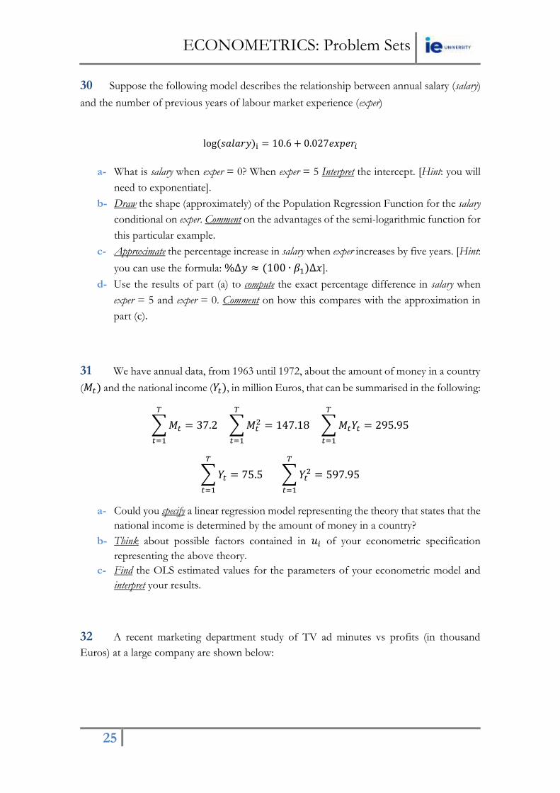
30 Suppose the following model describes the relationship between annual salary (salary)
and the number of previous years of labour market experience (exper)
log (𝑠𝑎𝑙𝑎𝑟𝑦)i = 10.6 + 0.027𝑒𝑥𝑝𝑒𝑟𝑖
a- What is salary when exper = 0? When exper = 5 Interpret the intercept. [Hint: you will
need to exponentiate].
b- Draw the shape (approximately) of the Population Regression Function for the salary
conditional on exper. Comment on the advantages of the semi-logarithmic function for
this particular example.
c- Approximate the percentage increase in salary when exper increases by five years. [Hint:
you can use the formula: %∆𝑦 ≈ (100 ∙ 𝛽1)∆𝑥].
d- Use the results of part (a) to compute the exact percentage difference in salary when
exper = 5 and exper = 0. Comment on how this compares with the approximation in
part (c).
31 We have annual data, from 1963 until 1972, about the amount of money in a country
(𝑀𝑡) and the national income (𝑌𝑡), in million Euros, that can be summarised in the following:
∑ 𝑀𝑡 = 37.2 ∑ 𝑀𝑡2 = 147.18 ∑ 𝑀𝑡𝑌𝑡 = 295.95
𝑇
𝑡=1
𝑇
𝑡=1
𝑇
𝑡=1
∑ 𝑌𝑡 = 75.5 ∑ 𝑌𝑡2 = 597.95
𝑇
𝑡=1
𝑇
𝑡=1
a- Could you specify a linear regression model representing the theory that states that the
national income is determined by the amount of money in a country?
b- Think about possible factors contained in 𝑢𝑖 of your econometric specification
representing the above theory.
c- Find the OLS estimated values for the parameters of your econometric model and
interpret your results.
32 A recent marketing department study of TV ad minutes vs profits (in thousand
Euros) at a large company are shown below:

ECONOMETRICS: Problem Sets
26
TV Ad Minutes Money earned from Ad time
11 80
8 60
15 55
10 62
The average of TV Ad Minutes is 11; the average of money earned from Ad time is 64.25.
The standard deviation of TV Ad minutes is 2.94 and the standard deviation of money
earned from Ad time is 10.9. The covariance between variables is -7.33.
a- Draw a scatter plot and interpret it.
b- Determine the regression equation. What is the interpretation of ��0 and��1?
c- How much profit does the company make if they advertise for 20 minutes in a
month?
d- R-Squared is 0.05, what does this mean?
33 One company in the aeronautics industry wants to calculate the number of working
hours that are required to finish the design of a new airplane. They think that the relevant
explanatory variables are the top speed of the airplane, its weight and the number of pieces
that are shared with other airplane models that the company builds. In order to do this, a
sample of 35 airplanes is taken and the following model is estimated:
𝑦𝑖 = 𝛽0 + 𝛽1𝑥1𝑖 + 𝛽2𝑥2𝑖 + 𝛽3𝑥3𝑖 + 𝑢𝑖
Such that:
𝑦𝑖= design effort in million working hours.
𝑥1𝑖= airplane´s top speed in kilometres per hour.
𝑥2𝑖= airplane´s weight in tons.
𝑥3𝑖= percent number of pieces that are shared with other airplane models.
The estimated regression coefficients are:
��1 = 0.661 ; ��2 = 0.065 ; ��3 = −0.018
Interpret the above estimated values.
ECONOMETRICS: Problem Sets
27
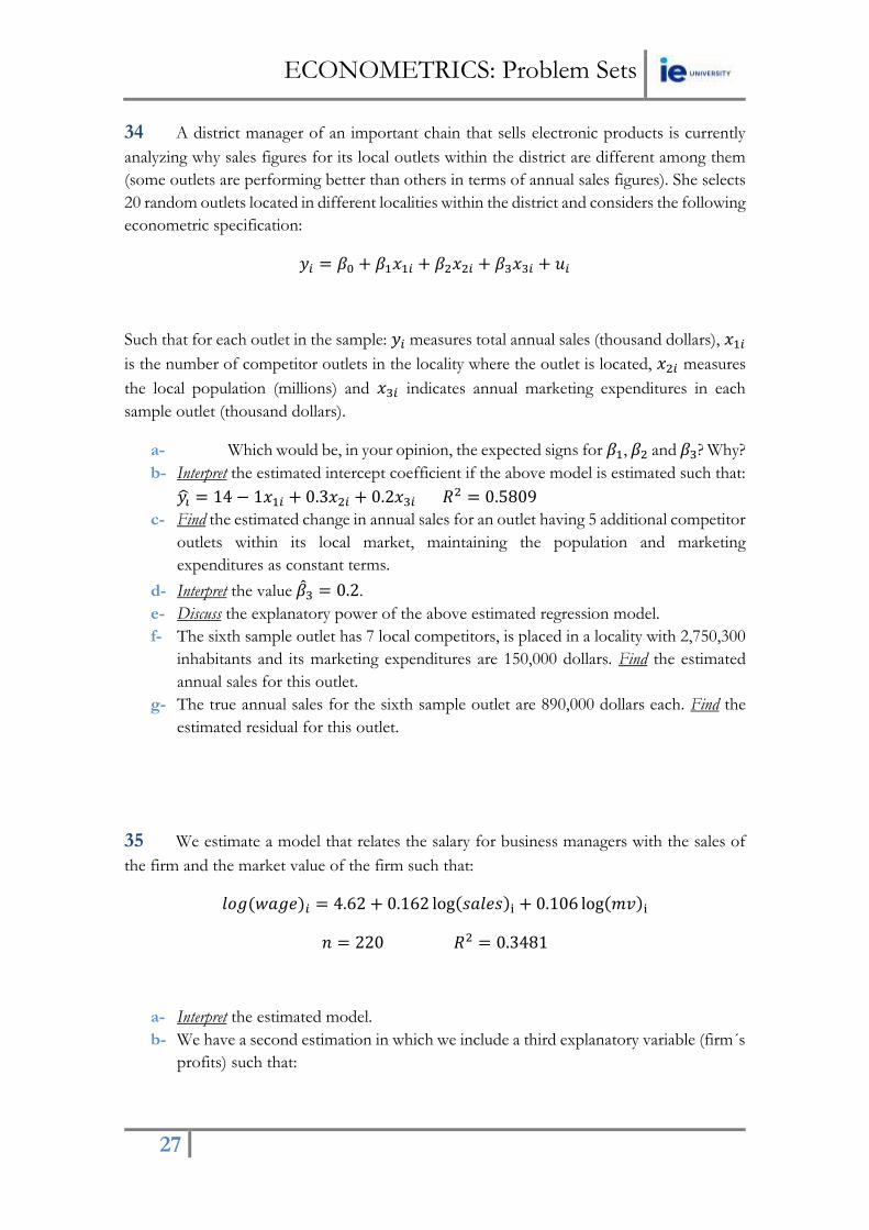
34 A district manager of an important chain that sells electronic products is currently
analyzing why sales figures for its local outlets within the district are different among them
(some outlets are performing better than others in terms of annual sales figures). She selects
20 random outlets located in different localities within the district and considers the following
econometric specification:
𝑦𝑖 = 𝛽0 + 𝛽1𝑥1𝑖 + 𝛽2𝑥2𝑖 + 𝛽3𝑥3𝑖 + 𝑢𝑖
Such that for each outlet in the sample: 𝑦𝑖 measures total annual sales (thousand dollars), 𝑥1𝑖
is the number of competitor outlets in the locality where the outlet is located, 𝑥2𝑖 measures
the local population (millions) and 𝑥3𝑖 indicates annual marketing expenditures in each
sample outlet (thousand dollars).
a- Which would be, in your opinion, the expected signs for 𝛽1, 𝛽2 and 𝛽3? Why?
b- Interpret the estimated intercept coefficient if the above model is estimated such that:
𝑦�� = 14 − 1𝑥1𝑖 + 0.3𝑥2𝑖 + 0.2𝑥3𝑖 𝑅2 = 0.5809
c- Find the estimated change in annual sales for an outlet having 5 additional competitor
outlets within its local market, maintaining the population and marketing
expenditures as constant terms.
d- Interpret the value ��3 = 0.2.
e- Discuss the explanatory power of the above estimated regression model.
f- The sixth sample outlet has 7 local competitors, is placed in a locality with 2,750,300
inhabitants and its marketing expenditures are 150,000 dollars. Find the estimated
annual sales for this outlet.
g- The true annual sales for the sixth sample outlet are 890,000 dollars each. Find the
estimated residual for this outlet.
35 We estimate a model that relates the salary for business managers with the sales of
the firm and the market value of the firm such that:
𝑙𝑜𝑔 (𝑤𝑎𝑔𝑒)𝑖 = 4.62 + 0.162 log(𝑠𝑎𝑙𝑒𝑠)i + 0.106 log(𝑚𝑣)i
𝑛 = 220 𝑅2 = 0.3481
a- Interpret the estimated model.
b- We have a second estimation in which we include a third explanatory variable (firm´s
profits) such that:

ECONOMETRICS: Problem Sets
28
log(𝑤𝑎𝑔𝑒)i = 4.734 + 0.165 log(𝑠𝑎𝑙𝑒𝑠)i + 0.084 log(𝑚𝑣)i + 0.003𝑝𝑟𝑜𝑓𝑖𝑡𝑠𝑖
𝑛 = 220 𝑅2 = 0.3541
Why 𝑝𝑟𝑜𝑓𝑖𝑡𝑠𝑖 variable is not included in the model in logs? Which is the model with
a better goodness-of-fit? Do these firm specific variables explain the behaviour of
the wage variable? Why?
36 Consider the regression model in which the dependent variable (television viewing
hours per week) is to be explained in terms of three explanatory variables:
𝑦𝑖 = 𝛽0 + 𝛽1𝑥1𝑖 + 𝛽2𝑥2𝑖 + 𝛽3𝑥3𝑖 + 𝑢𝑖
Such that:
𝑥1𝑖= income in thousand Dollars.
𝑥2𝑖= hours per week spent at work.
𝑥3𝑖= number of people living in the household.
The estimated regression coefficients are:
��1 = −1.28 ; ��2 = −0.13 ; ��3 = 2.45
Interpret the above estimated values.
37 Assume that we have the following theoretical specification:
𝑦𝑖= 𝛽0 + 𝛽1𝑥1𝑖 + 𝛽2𝑥1𝑖2 + 𝑢𝑖
Explain, in your opinion, whether the following statements are true or false:
a- One unit change in 𝑥1𝑖 always produces the same effect on the value of the
independent variable.
b- One unit change in 𝑥1𝑖 does not produce the same effect on y, but depends on the
value of 𝑥1𝑖.

ECONOMETRICS: Problem Sets
29
38 A company in the financial sector wants to rent an office space in Madrid. The
following regression model estimates the rent prices for office space in Madrid:
𝑝𝑟𝑖𝑐𝑒𝑖 = 𝛽0 + 𝛽1𝑠𝑞𝑓𝑒𝑒𝑡𝑖 + 𝛽2𝑑𝑖𝑠𝑖 + 𝑢𝑖
Such that sqfeet is the office space in square feet, dis is the distance between the place the
office is located and the city centre, measured in kilometres, and price is the monthly rental
price in thousand Euros.
a- Which would be the expected signs for 𝛽1 and 𝛽2? Why?
b- The above model is estimated such that:
𝑝𝑟𝑖𝑐𝑒𝑖 = −19.315 + 1.1284𝑠𝑞𝑓𝑒𝑒𝑡𝑖 − 0.8819𝑑𝑖𝑠𝑖
𝑛 = 120 𝑅2 = 0.6319
Interpret the constant term.
c- Find the estimated increment in the rental price for an office space with 100
additional square feet, maintaining the distance to the city centre as a constant term.
d- Find the change in the rental price for an office located 5 additional kilometres away
from the city centre, maintaining the size of the office as a constant term.
e- Discuss the explanatory power of the regression model.
f- The fifth sample office has a size of 120 square feet and is located at a distance of
5.4 kilometres from the city centre. Find the estimated rental price using the above
OLS regression line.
g- The true rental price for the fifth sample office is 89,000 Euros each month. Find the
estimated residual for this office. Could this suggest that the company is over paying
or under paying its office space?
39 A consultancy firm is analyzing monthly transportation costs in the manufacturing
sector for several companies. The following regression model estimates the transportation costs for a firm:
𝑡𝑐𝑖 = 𝛽0 + 𝛽1𝑜𝑖𝑙𝑝𝑖 + 𝛽2𝑑𝑖𝑠𝑖 + 𝑢𝑖
Such that oilp is the price of oil in Dollars per barrel, dis is the distance between the location of the manufacturing company and the location of its main supplier, measured in kilometers and tc denotes transportation costs in thousand Dollars.

ECONOMETRICS: Problem Sets
30
a- Which would be the expected signs for 𝛽1 and 𝛽2? Why? b- The above model is estimated such that:
𝑡𝑐�� = 23.385 + 10.588𝑜𝑖𝑙𝑝𝑖 + 0.777𝑑𝑖𝑠𝑖
𝑛 = 400 𝑅2 = 0.6319
Interpret the constant term. c- Find the estimated change in transportation costs if oil price decreases in 5 Dollars
per barrel, maintaining the distance to the main supplier as a constant term. d- Find the change in transportation costs for a company located 10 additional
kilometers away from its main supplier, maintaining oil price as a constant term. e- Discuss the explanatory power of the regression model. f- The tenth manufacturing firm pays oil at 97.16 Dollars per barrel and is located at a
distance of 23.4 kilometers from its main supplier. Find the estimated transportation costs using the above OLS regression line.
g- The true transportation costs for the tenth sample manufacturing firm is 28,000 Dollars each month. Find the estimated residual for this company.
40 The initial wage for just graduated lawyers is determined by the following estimated
regression model:
log(𝑤𝑎𝑔𝑒)𝑖 = 6.77 + 0.104 log(𝑏𝑜𝑜𝑘)𝑖 + 0.44 log(𝑐𝑜𝑠𝑡)𝑖
𝑛 = 200 𝑅2 = 0.278
Such that 𝑤𝑎𝑔𝑒𝑖 measures initial monthly wage in thousand Euros, 𝑏𝑜𝑜𝑘𝑖 indicates the
number of law books in the university library where the graduated studied and 𝑐𝑜𝑠𝑡𝑖
measures the annual cost (thousand Euros) of the university where the graduated got her law
title.
a- Interpret the above estimated model.
b- We have a second estimation in which we include a third explanatory variable: rank
of the law faculty (being 𝑟𝑎𝑛𝑘 = 1 the best one) such that:
log(𝑤𝑎𝑔𝑒)i = 6.34 + 0.095 log(𝑏𝑜𝑜𝑘)i + 0.38 log(𝑐𝑜𝑠𝑡)i − 0.0033𝑟𝑎𝑛𝑘𝑖
𝑛 = 200 𝑅2 = 0.294
Why 𝑟𝑎𝑛𝑘𝑖 variable is not included in the model in logs? Which is the model with a better
goodness-of-fit? Do these university specific variables explain the behaviour of the wage
variable? Why?

ECONOMETRICS: Problem Sets
31
41 A consultancy firm is analyzing property prices in the city of Madrid using a sample
of 88 properties using the following regression model:
𝑝𝑖 = 𝛽0 + 𝛽1𝑠𝑞𝑟𝑓𝑡𝑖 + 𝛽2𝑏𝑑𝑟𝑚𝑠𝑖 + 𝑢𝑖
Such that p is property price in thousand dollars, sqrft is the size of the property in squared
feet, and bdrms is the number of bedrooms.
a- Which would be the expected signs for 𝛽1 and 𝛽2? Why?
b- The above model is estimated such that:
𝑝�� = −19.315 + 0.128𝑠𝑞𝑟𝑓𝑡𝑖 + 15.198𝑏𝑑𝑟𝑚𝑠𝑖
𝑛 = 88 𝑅2 = 0.6319
Interpret the constant term.
c- Find the estimated change in property prices if there is an increment of 3 bedrooms,
maintaining the size of the property as a constant term.
d- Find the change in property prices for each additional 10 square feet in size,
maintaining the number of bedrooms as a constant term.
e- Discuss the explanatory power of the regression model (goodness-of-fit).
f- The tenth property has a size of 2,438 square feet and has 4 bedrooms. Find the
estimated property price using the above OLS regression line.
g- The true property price for the tenth sample property is 300,000 Dollars. Find the
estimated residual for this company. Does this suggest that the buyer underpaid this
property?
42 Consider Y (logarithm of real money demand), X1 (logarithm of real GDP) and X2
(logarithm of the interest rate of Treasury bills). Consider the following regression results:
𝑌�� = 2.3296 + 0,5573𝑋1𝑖 − 0.2032𝑋2𝑖
Interpret the above estimated equation.
43 The CEO salary is determined by the following estimated regression model:
log(𝑠𝑎𝑙𝑎𝑟𝑦)𝑖 = 6.77 + 0.904 log(𝑠𝑎𝑙𝑒𝑠)𝑖 + 1.44𝑐𝑒𝑜𝑡𝑒𝑛𝑖
𝑛 = 400 𝑅2 = 0.388

ECONOMETRICS: Problem Sets
32
Such that 𝑠𝑎𝑙𝑎𝑟𝑦𝑖 measures monthly wage in thousand Euros, 𝑠𝑎𝑙𝑒𝑠𝑖 indicates monthly firm
sales in thousand Euros and 𝑐𝑒𝑜𝑡𝑒𝑛𝑖 measures CEO tenure with the firm in years.
a- Interpret the above estimated model.
b- Why 𝑐𝑒𝑜𝑡𝑒𝑛𝑖 variable is not included in the model in logs?
We re-estimate the above model including a new explanatory factor, CEO education in years
and we obtain the following estimation results:
log(𝑠𝑎𝑙𝑎𝑟𝑦)𝑖 = 5.77 + 0.774 log(𝑠𝑎𝑙𝑒𝑠)𝑖 + 1.15𝑐𝑒𝑜𝑡𝑒𝑛𝑖 + 0.54𝑐𝑒𝑜𝑒𝑑𝑢𝑖
𝑛 = 400 𝑅2 = 0.498
c- Which is the model with a better goodness-of-fit? Why?
44 The Data on U.S. working men was used to estimate the following equation:
𝑒𝑑𝑢𝑐𝑖 = 10.30 − 0.094𝑠𝑖𝑏𝑠𝑖 + 0.131𝑚𝑒𝑑𝑢𝑐𝑖 + 0.210𝑓𝑒𝑑𝑢𝑐𝑖
𝑛 = 722 𝑅2 = 0.214
where educ is years of schooling, sibs is number of siblings, meduc is mother’s years of
schooling, and feduc is father’s years of schooling.
a- Does sibs have the expected effect? Explain. Holding meduc and feduc fixed, by how
much does sibs have to increase to reduce predicted years of education by one year?
(A non-integer answer is acceptable here)
b- Discuss the interpretation of the coefficient on meduc.
c- Suppose that Man A has no siblings, and his mother and father each have 12 years
of education. Man B has no siblings, and his mother and father each have 16 years
of education. What is the predicted difference in educ between A and B?
d- Would you say sibs, meduc and feduc explain much of the variation in educ? What other
factors might affect men’s years of schooling? Are these likely to be correlated with
sibs? Explain.
45 For a child 𝑖 living in a particular school district, let 𝑣𝑜𝑢𝑐ℎ𝑒𝑟𝑖 be a dummy variable
equal to one if a child is selected to participate in a school voucher program, and let 𝑠𝑐𝑜𝑟𝑒𝑖
be that child’s score on a subsequent standardized exam. Suppose that the participation

ECONOMETRICS: Problem Sets
33
variable, 𝑣𝑜𝑢𝑐ℎ𝑒𝑟𝑖 , is completely randomized in the sense that it is independent of both
observed and unobserved factors that can affect the test score.
a- If you run a simple regression 𝑠𝑐𝑜𝑟𝑒𝑖 on 𝑣𝑜𝑢𝑐ℎ𝑒𝑟𝑖, using a random sample of size
𝑛, which sign do you expect to find on the coefficient associated to the dummy
variable? Explain the intuition.
b- Does the OLS estimator provide an unbiased estimator of the effect of the voucher
program?
c- Suppose you can collect additional background information, such as family income,
family structure and parent’s education levels. Do you need to control for these
factors to obtain an unbiased estimator of the effects of the voucher program?
Explain.
46 Observe the equation below:
𝑦 = 𝛽0 + 𝛽1𝑥1 + 𝛽2𝑥2 + 𝛽3𝑥3 + 𝑢
Write and explain at least three characteristics that this model need to have to not violate
Gauss-Markov theorem.
47 Consider the multiple regression model containing three independent variables, under
Assumptions MLR.1 through MLR.4:
𝑦 = 𝛽0 + 𝛽1𝑥1 + 𝛽2𝑥2 + 𝛽3𝑥3 + 𝑢
You are interested in estimating the sum of the parameters on 𝑥1 and 𝑥2; call this 𝜃1 = 𝛽1 +
𝛽2
a- Show that 𝜃1 = ��1 + ��2 is an unbiased estimator of 𝜃1.
b- Find 𝑉𝑎𝑟(𝜃1) in terms of 𝑉𝑎𝑟(��1), 𝑉𝑎𝑟(��2) and 𝐶𝑜𝑟𝑟(��1, ��2)
ECONOMETRICS: Problem Sets
34
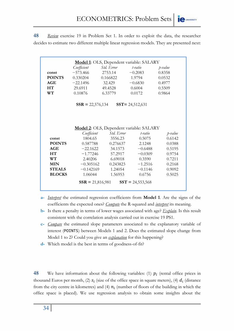
48 Review exercise 19 in Problem Set 1. In order to exploit the data, the researcher
decides to estimate two different multiple linear regression models. They are presented next:
Model 1: OLS, Dependent variable: SALARY Coefficient Std. Error t-ratio p-value
const −573.466 2753.14 −0.2083 0.8358 POINTS 0.330204 0.166822 1.9794 0.0532 AGE −22.1496 32.429 −0.6830 0.4977 HT 29.6911 49.4528 0.6004 0.5509 WT 0.10876 6.33779 0.0172 0.9864
SSR = 22,576,134 SST= 24,512,631
Model 2: OLS, Dependent variable: SALARY Coefficient Std. Error t-ratio p-value
const 1804.65 3556.23 0.5075 0.6142 POINTS 0.587788 0.276637 2.1248 0.0388 AGE −22.1622 34.1573 −0.6488 0.5195 HT −1.77246 57.2917 −0.0309 0.9754 WT 2.40206 6.69018 0.3590 0.7211 MIN −0.305162 0.243823 −1.2516 0.2168 STEALS −0.142169 1.24054 −0.1146 0.9092 BLOCKS 1.06044 1.56953 0.6756 0.5025
SSR = 21,816,981 SST = 24,553,568
a- Interpret the estimated regression coefficients from Model 1. Are the signs of the
coefficients the expected ones? Compute the R-squared and interpret its meaning.
b- Is there a penalty in terms of lower wages associated with age? Explain. Is this result
consistent with the correlation analysis carried out in exercise 19 PS1.
c- Compare the estimated slope parameters associated to the explanatory variable of
interest (POINTS) between Models 1 and 2. Does the estimated slope change from
Model 1 to 2? Could you give an explanation for this happening?
d- Which model is the best in terms of goodness-of-fit?
48 We have information about the following variables: (1) 𝑝𝑖 (rental office prices in
thousand Euros per month, (2) 𝑠𝑖 (size of the office space in square meters), (4) 𝑑𝑖 (distance
from the city centre in kilometres) and (4) 𝑛𝑖 (number of floors of the building in which the
office space is placed). We use regression analysis to obtain some insights about the

ECONOMETRICS: Problem Sets
35
behaviour of rental office prices using a sample of 150 offices located within the city of
Barcelona in 2012. You can see in the below table estimation results:
Table 1: OLS Estimation Results
Model 1 Model 2 Model 3 Model 4
Variable coefficients coefficients coefficients coefficients
constant -34.65 1.58 1.22 0.38
size 0.076 0.025 0.022 0.042
distance -0.098 -0.088 numfloors -0.127 log(distance) -3.14
n 150 150 150 150
R squared 0.243 0.457 0.422 0.527
Note: Models 1, 2 and 3 use as dependent variable prices and Model 4 uses as dependent
variable log(prices).
a- What happens to the coefficient of size when comparing Model 1 and Model 2?
Why?
b- Which model do you prefer when comparing Model 1 and Model 2?
c- Do you think Model 3 is a better specification than Model 2? Why?
d- Interpret the coefficients associated to Model 4?
e- Is Model 4 the best model? Why?

ECONOMETRICS: Problem Sets
36
PS3
Hypothesis
Testing
COURSE CONTENT
-Chapter 5: Hypothesis Testing
-Hypothesis Testing in the SLRM.
-Hypothesis Testing in the MLRM.
Three econometricians went out hunting, and came across a large deer. The first econometrician fired, but missed, by a meter to the left. The second econometrician fired, but also missed, by a meter to the right. The
third econometrician didn't fire, but shouted in triumph, "We got it! We got it!"

ECONOMETRICS: Problem Sets
37
1 We are interested in examining the relationship between Cabinet duration and
Polarization where 𝐶𝐷𝑖 denotes the number of months a cabinet government survives until
its fall (this variable ranges from 0.5, half a month, to 59 months) and 𝑃𝑖 measures the
support in the country for extremist political parties (this variable ranges from 0, 0%, to 43,
43% support. It is hypothesized that polarization will be negatively related to cabinet
duration: the more support there is for extremist parties, the more difficult it will become
for the governing party to bargain and hence, maintain a government. The sample size is 314
and OLS estimation result is the following (standard errors in parenthesis):
𝐶𝐷𝑖 = 26.652 − 0.537𝑃𝑖 𝑅
2 = 0.41
(1.189) (0.06)
a- Interpret the estimated regression model and the value of the determination coefficient
b- Test the null hypothesis that the polarisation coefficient is zero at a 1% significance
level.
c- Knowing that a country has a 25% support for extremist parties, find the predicted
cabinet duration.
d- In your opinion, explain one application of the above model from the perspective of
a non-extremist political party.
2 Annual profits evolution in an Italian company in the aeronautics sector follows an
exponential growth model which was estimated for the time period 1981-2010 (both years
included in the sample) such that:
𝑙𝑜𝑔𝑦�� = 32.555 + 0.0534𝑡
(33.2) (0.00211)
a- Interpret the estimated slope coefficient.
b- Test the null hypothesis that the true value for the slope coefficient is zero at a 5%
significance level. What about at 1% significance level? Which of the two t-test is
more informative?
3 Population time evolution in the United States follows an exponential growth model
which was estimated for the time period 1970-1999 (both years included in the sample) such
that:
𝑙𝑜𝑔𝑦�� = 201.9727 + 0.0284𝑡
(743.2) (0.00211)

ECONOMETRICS: Problem Sets
38
a- Interpret the estimated slope coefficient.
b- Test the null hypothesis that the true value for the slope coefficient is zero at a 5%
significance level. What about at 1% significance level?
c- In your opinion, could you use the above model to predict the United States´
population in the current decade? Why?
4 Consider a SLRM relating the annual number of crimes on college campuses (crime) to
student enrollment (enroll) with the following estimation results:
log (𝑐𝑟𝑖𝑚𝑒)𝑖 = −6.63 + 1.27log (𝑒𝑛𝑟𝑜𝑙𝑙)𝑖 𝑛 = 97 𝑅2 = 0.585
(1.03) (0.11)
a- Interpret the estimated slope coefficient.
b- Calculate two-tailed test to find whether the variable enroll should be included in the
regression model (at 1% significance level).
c- Test that the elasticity of crime with respect to enrolment is 1 (at 5% significance
level).
d- What could you say about the explanatory power of the above model? Test the whole
model fit at 5% significance level.
5 We have a sample 𝑇 = 27 with data for the following variables:
Y: housing expenditure in USA (dollars)
X: household income (dollars)
The following regression model is estimated through OLS:
𝑙𝑜𝑔𝑦�� = 1.20 + 0.55𝑙𝑜𝑔𝑥𝑡 𝑆𝑆𝑇 = 330 𝑆𝑆𝑅 = 51
(0.11) (0.02)
a- Interpret the estimated slope coefficient.
b- Calculate one-tailed test to find whether the variable 𝑙𝑜𝑔𝑥𝑡 should be included in the
regression model (at 1% significance level).
c- Test that housing expenditure elasticity respect to household income is 1 (at 5%
significance level).
d- What could you say about the explanatory power of the above model? Test the whole
model fit at 5% significance level.

ECONOMETRICS: Problem Sets
39
6 Given the following regression model:
𝐼𝑛𝑓𝑙𝑎𝑡𝑖𝑜𝑛𝑖 = 𝛽0 + 𝛽1𝐼𝑛𝑡𝑒𝑟𝑒𝑠𝑡𝑅𝑎𝑡𝑒𝑖 + 𝑢𝑖
Where both variables are measured in percentage points, a sample of 100 countries is used
in order to estimate the above model and the following information is given:
𝑉𝑎𝑟(𝐼𝑛𝑓𝑙𝑎𝑡𝑖𝑜𝑛𝑖) = 100; 𝑉𝑎𝑟(𝐼𝑛𝑡𝑒𝑟𝑒𝑠𝑡𝑅𝑎𝑡𝑒𝑖) = 50;
𝐶𝑜𝑣(𝐼𝑛𝑓𝑙𝑎𝑡𝑖𝑜𝑛𝑖, 𝐼𝑛𝑡𝑒𝑟𝑒𝑠𝑡𝑅𝑎𝑡𝑒𝑖) = −25; 𝑆𝑆𝑅 = 49
a- Find the OLS estimation of the effect of interest rates on inflation and the estimated
standard error.
b- Interpret your estimation results.
c- Calculate a one-tailed t-test in order to validate the significance of the estimated slope
coefficient at 1% significance level.
d- What could you say about the explanatory power of the above model? Test the whole
model fit at 5% significance level.
7 We have a sample of 45 workers employed in a company. We ask to each worker to
evaluate her/his satisfaction level at work (x) from 0 to 10. We also know, for each worker,
the number of labor absenteeism days (y) last year. A linear regression line is estimated such
that:
𝑦�� = 12.6 − 1.2𝑥𝑖 𝑅2 = 0.321
(0.112) (0.088)
a- Interpret the estimated regression model and the value of the determination coefficient
b- Test the null hypothesis that work satisfaction does not produce any significant effect
on labour absenteeism at a 1% significance level.
c- The level of work satisfaction of a different worker is 6. Find the predicted labour
absenteeism days per year for this worker.
d- In your opinion, explain one application of the above model from the perspective of
the Human Resources department of the company.
ECONOMETRICS: Problem Sets
40
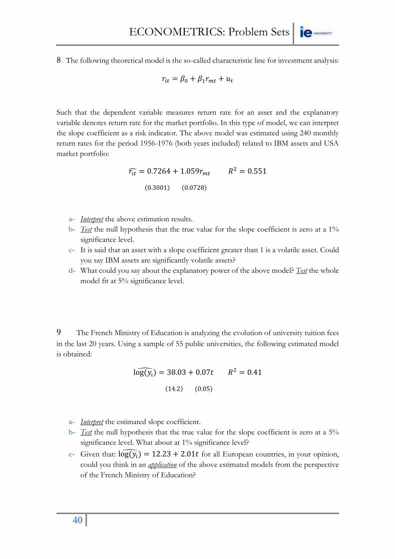
8 The following theoretical model is the so-called characteristic line for investment analysis:
𝑟𝑖𝑡 = 𝛽0 + 𝛽1𝑟𝑚𝑡 + 𝑢𝑡
Such that the dependent variable measures return rate for an asset and the explanatory
variable denotes return rate for the market portfolio. In this type of model, we can interpret
the slope coefficient as a risk indicator. The above model was estimated using 240 monthly
return rates for the period 1956-1976 (both years included) related to IBM assets and USA
market portfolio:
𝑟𝑖�� = 0.7264 + 1.059𝑟𝑚𝑡 𝑅2 = 0.551
(0.3001) (0.0728)
a- Interpret the above estimation results.
b- Test the null hypothesis that the true value for the slope coefficient is zero at a 1%
significance level.
c- It is said that an asset with a slope coefficient greater than 1 is a volatile asset. Could
you say IBM assets are significantly volatile assets?
d- What could you say about the explanatory power of the above model? Test the whole
model fit at 5% significance level.
9 The French Ministry of Education is analyzing the evolution of university tuition fees
in the last 20 years. Using a sample of 55 public universities, the following estimated model
is obtained:
log (𝑦𝑖) = 38.03 + 0.07𝑡 𝑅2 = 0.41
(14.2) (0.05)
a- Interpret the estimated slope coefficient.
b- Test the null hypothesis that the true value for the slope coefficient is zero at a 5%
significance level. What about at 1% significance level?
c- Given that: log (𝑦𝑖) = 12.23 + 2.01𝑡 for all European countries, in your opinion,
could you think in an application of the above estimated models from the perspective
of the French Ministry of Education?

ECONOMETRICS: Problem Sets
41
10 The OLS estimation for a model that relates annual household expenditures in
thousand Euros (𝐺𝑖) with annual household disposable income in thousand Euros (𝐼𝑖) and
number of individuals within the household (𝑁𝑖) is given by the following regression line
(𝑛 = 38 households):
𝐺�� = 2.24 + 0.16𝐼𝑖 + 1.45𝑁𝑖 𝑅2 = 0.45
(2.666) (0.0345) (0.5253)
a- Test the individual significance of each explanatory variable at 5% significance level.
b- Test the overall significance of the model at 5% significance level.
c- Test if the coefficient associated to 𝑁𝑖 equals to one at 5% significance level.
d- Interpret the value of the determination coefficient. What would you change in the
above specification in order to increase the explanatory power of the model?
11 An econometric study for the period 1960-2004 relates production costs in USA (y)
and time (x) such that t=1 (1960), t=2 (1962), and ... t=23 (2004). The following exponential
model is obtained:
log (𝑦𝑡) = 95.3 + 0.0253𝑡
(4.15) (0.008)
a- Interpret the estimated slope coefficient.
b- Test the null hypothesis that the true value for the slope coefficient is zero at a 5%
significance level.
c- Test the above but at a 1% significance level. Why this second hypothesis test is more
informative than the first one?
12 Are rent rates influenced by the student population in a college town? Let rent be the
average monthly rent paid on rental units in a college town. Let pop denote the total city
population, avginc the average city income, and pctstu the student population as a percent of
the total population. We get the following estimation results:
log (𝑟𝑒𝑛𝑡)𝑡 = −0.043 + 0.066log (𝑝𝑜𝑝)𝑡 + 0.507log (𝑎𝑣𝑔𝑖𝑛𝑐)𝑡 + 0.0056𝑝𝑐𝑡𝑠𝑡𝑢𝑡
(0.844) (0.039) (0.081) (0.0056)
𝑅2 = 0.458 𝑇 = 64
ECONOMETRICS: Problem Sets
42
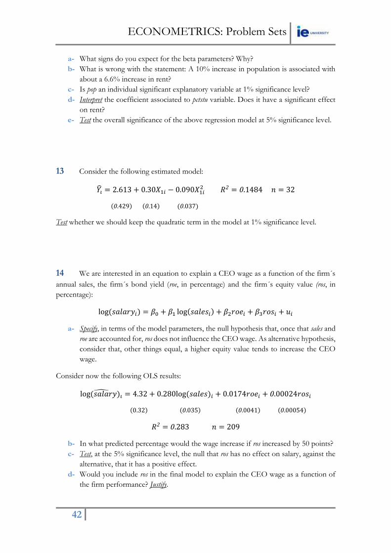
a- What signs do you expect for the beta parameters? Why?
b- What is wrong with the statement: A 10% increase in population is associated with
about a 6.6% increase in rent?
c- Is pop an individual significant explanatory variable at 1% significance level?
d- Interpret the coefficient associated to pctstu variable. Does it have a significant effect
on rent?
e- Test the overall significance of the above regression model at 5% significance level.
13 Consider the following estimated model:
𝑌�� = 2.613 + 0.30𝑋1𝑖 − 0.090𝑋1𝑖2 𝑅2 = 0.1484 𝑛 = 32
(0.429) (0.14) (0.037)
Test whether we should keep the quadratic term in the model at 1% significance level.
14 We are interested in an equation to explain a CEO wage as a function of the firm´s
annual sales, the firm´s bond yield (roe, in percentage) and the firm´s equity value (ros, in
percentage):
log (𝑠𝑎𝑙𝑎𝑟𝑦𝑖) = 𝛽0 + 𝛽1 log(𝑠𝑎𝑙𝑒𝑠𝑖) + 𝛽2𝑟𝑜𝑒𝑖 + 𝛽3𝑟𝑜𝑠𝑖 + 𝑢𝑖
a- Specify, in terms of the model parameters, the null hypothesis that, once that sales and
roe are accounted for, ros does not influence the CEO wage. As alternative hypothesis,
consider that, other things equal, a higher equity value tends to increase the CEO
wage.
Consider now the following OLS results:
log (𝑠𝑎𝑙𝑎𝑟𝑦)𝑖 = 4.32 + 0.280log (𝑠𝑎𝑙𝑒𝑠)𝑖 + 0.0174𝑟𝑜𝑒𝑖 + 0.00024𝑟𝑜𝑠𝑖
(0.32) (0.035) (0.0041) (0.00054)
𝑅2 = 0.283 𝑛 = 209
b- In what predicted percentage would the wage increase if ros increased by 50 points?
c- Test, at the 5% significance level, the null that ros has no effect on salary, against the
alternative, that it has a positive effect.
d- Would you include ros in the final model to explain the CEO wage as a function of
the firm performance? Justify.

ECONOMETRICS: Problem Sets
43
15 Using a dataset for 46 states of the United States in 1992, the following estimated
regression line was obtained:
𝑙𝑜𝑔𝐶𝑖 = 4.30 − 1.34𝑙𝑜𝑔𝑃𝑖 + 0.17𝑙𝑜𝑔𝑌𝑖 𝑅2 = 0.37
(0.91) (0.32) (0.20)
Such that:
𝐶𝑖 denotes cigarettes consumption (number of packets per year).
𝑃𝑖 measures price per packet (dollars).
𝑌𝑖 denotes average annual income in state i (thousand dollars)
a- Find the elasticity of cigarettes consumption respect to price. Is it statistically
significant at 1% significance level? If it is statistically significant, is it statistically
different to -1 at 1% significance level?
b- Find the elasticity of cigarettes consumption respect to income. Is it statistically
significant at 1% significance level? If it is not statistically significant, in your opinion,
explain why.
c- Find the value for the determination coefficient. Interpret its value and test the overall
significance of the model at 1% significance level.
16 The goal of this exercise is to test the rationality of assessments of housing prices.
We use a model that relates the assessment of the house with its price for a sample of 88
houses.
a- In the SLRM:
𝑝𝑟𝑖𝑐𝑒𝑖 = 𝛽0 + 𝛽1𝑎𝑠𝑠𝑒𝑠𝑠𝑖 + 𝑢𝑖
the assessment is rational if 𝛽0 = 0 and 𝛽1 = 0. The estimated equation is:
𝑝𝑟𝑖𝑐�� = −14.47 + 0.976𝑎𝑠𝑠𝑒𝑠𝑠𝑖 𝑅2 = 0.82 𝑆𝑆𝑅 = 165,644.
(16.27) (0.049)
First, test whether assess is a significant variable at 5% significance level. Then, test 𝐻0: 𝛽1 =
1 . What do you conclude?
c- Now test whether the addition of new variables in the model below is a significant
improvement respect the first model:
𝑝𝑟𝑖𝑐𝑒𝑖 = 𝛽0 + 𝛽1𝑎𝑠𝑠𝑒𝑠𝑠𝑖 + 𝛽2𝑙𝑜𝑡𝑠𝑖𝑠𝑒𝑖 + 𝛽3𝑠𝑞𝑟𝑓𝑖 + 𝛽4𝑏𝑑𝑟𝑚𝑠𝑖 + 𝑢𝑖
Knowing that the determination coefficient of this model using the 88 houses is 0.829.

ECONOMETRICS: Problem Sets
44
17 For a sample of 506 communities in the Boston area, we estimate a model relating
median housing prices (price) in the community with two housing characteristics: dist is a
weighted distance of the community from five employment centres, in miles and rooms is the
average number of rooms in house in the community:
log(𝑟𝑒𝑛𝑡)𝑖 = 15.87 + 0.355𝑟𝑜𝑜𝑚𝑠𝑖 − 0.22 log(𝑑𝑖𝑠𝑡𝑖)
(0.342) (0.020) (0.055)
𝑅2 = 0.399 𝑛 = 506 𝑆𝑆𝑅 = 11.1
We try to improve the above specification by introducing two new independent factors
related to community characteristics: nox is the amount of nitrous oxide in the air, in parts
per million and stratio is the average student-teacher ratio of schools in the community:
log (𝑟𝑒𝑛𝑡)𝑖 = 11.8 + 0.25𝑟𝑜𝑜𝑚𝑠𝑖 − 0.13 log(𝑑𝑖𝑠𝑡𝑖) − 0.95 log(𝑛𝑜𝑥𝑖) − 0.052𝑠𝑡𝑟𝑎𝑡𝑖𝑜𝑖
(0.32) (0.019) (0.043) (0.117) (0.006)
𝑅2 = 0.506 𝑛 = 506 𝑆𝑆𝑅 = 4.88
a- Which is the most accurate model in terms of goodness-of-fit?
b- Test the joint significance of the two additional explanatory variables that are included
in the second model at 1% significance level.
18 We estimate a model aiming to study the annual salary, measured in thousand dollars
(1980-2007 time period) as a function of labor experience and education level, both of them
measured in years. The estimation results are the following:
𝑤�� = 100.25 + 0.87𝑙𝑒𝑡 + 1.85𝑒𝑑𝑢𝑡 𝑅2 = 0.95
(2.75) (0.025) (0.075)
a- Are the signs of the coefficients consistent with theory? Explain.
b- Interpret the explanatory power of the model.
c- Test the statistical significance of the model both individually and globally.

ECONOMETRICS: Problem Sets
45
19 We have the following equation representing the behavior of salaries in the British
economy for the time period 1950-1969:
𝑤�� = 1.073 + 0.288𝑣𝑡 + 0.116𝑥𝑡 + 0.054𝑚𝑡 + 0.056𝑚𝑡−1 𝑅2 = 0.934
(0.797) (0.812) (0.011) (0.022) (0.018)
Where:
𝑤𝑡: Salary per employee (thousand pounds).
𝑣𝑡 : Unemployment rate (percentage).
𝑥𝑡: GDP per head (thousand pounds).
𝑚𝑡: Import prices (,00 pounds per imported unit).
𝑚𝑡−1: Import prices lagged one period.
a- Interpret the estimated equation.
b- Find the explanatory variables that can be eliminated from the equation. Why?
c- Test the global significance of the model at 1% significance level.
20 A company in the railway transportation industry is analyzing the factors affecting
company´s income levels. Using a sample of 17 years, the following estimated regression
model is obtained:
�� = −2759.26 + 1.525𝑁 − 1.856𝐶 − 0.672𝐿 + 2.753𝑁𝐶
(2645.4) (0.402) (0.439) (0.369) (0.868)
𝑅2 = 0.879 𝑆𝑆𝑅 = 6.09
Where 𝑌 denotes annual income levels (thousand pounds), 𝑁 measures the number of trains
belonging to the company in each year, C is annual electricity consumption (thousand
pounds), L denotes annual labor costs (thousand pounds) and 𝑁𝐶 is total number of clients
in each year.
a- Test the individual significance of each explanatory variable at 5% significance level.
b- Test the overall significance of the model at 5% significance level.
c- Test if the coefficient associated to 𝑁 equals to one at 5% significance level.
d- Interpret the values of the determination coefficient and SSR.

ECONOMETRICS: Problem Sets
46
21 We have the following regression model:
𝑙𝑜𝑔𝑦𝑡 = 𝛽0 + 𝛽1𝑙𝑜𝑔𝑥1𝑡 + 𝛽2𝑙𝑜𝑔𝑥2𝑡 + 𝛽3𝑙𝑜𝑔𝑥3𝑡 + 𝑢𝑡
a- Analytically show that imposing the linear restriction 𝛽1 = −𝛽3, the model can be
rewritten as:
𝑙𝑜𝑔𝑦𝑡 = 𝛽0 + 𝛽2𝑙𝑜𝑔𝑥2𝑡 + 𝛽3𝑙𝑜𝑔𝑧𝑡 + 𝑢𝑡
Knowing that: 𝑧𝑡 =𝑥3𝑡
𝑥1𝑡
We estimate both models using 50 observations such that:
𝑙𝑜𝑔𝑦�� = 3.45 − 0.45𝑙𝑜𝑔𝑥1𝑡 + 0.28𝑙𝑜𝑔𝑥2𝑡 + 0.55𝑙𝑜𝑔𝑥3𝑡
(0.18) (0.81) (0.04) (0.02)
𝑆𝑆𝑅 = 0.186 𝑅2 = 0.47
And
𝑙𝑜𝑔𝑦�� = 0.29 + 0.87𝑙𝑜𝑔𝑥2𝑡 + 0.39𝑙𝑜𝑔𝑧𝑡
(0.17) (0.01) (0.05)
𝑆𝑆𝑅 = 0.204 𝑅2 = 0.8
b- Statistically validate the linear restriction at 1% significance level.
22 Consider the linear regression model:
𝑦𝑖 = 𝛽0 + 𝛽1𝑥1𝑖 + 𝛽2𝑥2𝑖 + 𝛽3𝑥3𝑖 + 𝛽4𝑥4𝑖 + 𝛽5𝑥5𝑖 + 𝑢𝑖
Explain how you would test the following hypothesis:
a- 𝛽1 = 0
b- 𝛽4 = 𝛽5
c- 𝛽3 = 𝛽4 = 𝛽5 = 0

ECONOMETRICS: Problem Sets
47
23 We have the following theoretical regression model:
𝑦𝑡 = 𝛼 + 𝛽𝑥𝑡 + 𝛾𝑧𝑡 + 𝛿𝑠𝑡 + 𝑢𝑡
We obtain the following estimated model through OLS using 10 observations:
𝑦�� = 4.1 + 2𝑥𝑡 + 0.4𝑧𝑡 + 0.35𝑠𝑡 𝑅2 = 0.79 𝑆𝑆𝑅 = 2
A new variable m is built such that:
𝑚𝑡 = 𝑧𝑡 + 𝑠𝑡
And a new theoretical model is defined:
𝑦𝑡 = �� + ��𝑥𝑡 + ��𝑚𝑡 + 𝑢𝑡
We estimate the above model such that:
𝑦�� = 4.0 + 1.8𝑥𝑡 + 0.47𝑚𝑡 𝑅2 = 0.77 𝑆𝑆𝑅 = 4
Test the null hypothesis that the coefficients for 𝑧𝑡 and 𝑠𝑡 are the same at 5% significance
level. What about at 1% significance level?
24 A marketing consultancy firm is investigating the behavior of sales in the pharmacy
industry. Using a sample of 75 companies within the industry, the following two regression
models are obtained:
𝑦�� = 22.163 + 0.363𝑥1𝑖 𝑅2 = 0.424 𝑆𝑆𝑅 = 78
(7.089) (0.0971)
𝑦�� = 7.059 + 1.0847𝑥1𝑖 − 0.004𝑥1𝑖2 − 0.245𝑥2𝑖 𝑅2 = 0.567 𝑆𝑆𝑅 = 47
(9.986) (0.3699) (0.0019) (0.111)
ECONOMETRICS: Problem Sets
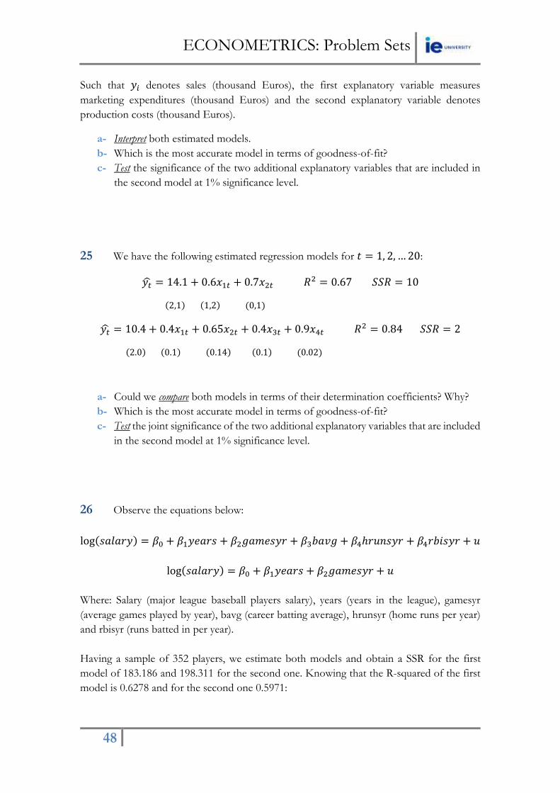
48
Such that 𝑦𝑖 denotes sales (thousand Euros), the first explanatory variable measures
marketing expenditures (thousand Euros) and the second explanatory variable denotes
production costs (thousand Euros).
a- Interpret both estimated models.
b- Which is the most accurate model in terms of goodness-of-fit?
c- Test the significance of the two additional explanatory variables that are included in
the second model at 1% significance level.
25 We have the following estimated regression models for 𝑡 = 1, 2, … 20:
𝑦�� = 14.1 + 0.6𝑥1𝑡 + 0.7𝑥2𝑡 𝑅2 = 0.67 𝑆𝑆𝑅 = 10
(2,1) (1,2) (0,1)
𝑦�� = 10.4 + 0.4𝑥1𝑡 + 0.65𝑥2𝑡 + 0.4𝑥3𝑡 + 0.9𝑥4𝑡 𝑅2 = 0.84 𝑆𝑆𝑅 = 2
(2.0) (0.1) (0.14) (0.1) (0.02)
a- Could we compare both models in terms of their determination coefficients? Why?
b- Which is the most accurate model in terms of goodness-of-fit?
c- Test the joint significance of the two additional explanatory variables that are included
in the second model at 1% significance level.
26 Observe the equations below:
log(𝑠𝑎𝑙𝑎𝑟𝑦) = 𝛽0 + 𝛽1𝑦𝑒𝑎𝑟𝑠 + 𝛽2𝑔𝑎𝑚𝑒𝑠𝑦𝑟 + 𝛽3𝑏𝑎𝑣𝑔 + 𝛽4ℎ𝑟𝑢𝑛𝑠𝑦𝑟 + 𝛽4𝑟𝑏𝑖𝑠𝑦𝑟 + 𝑢
log(𝑠𝑎𝑙𝑎𝑟𝑦) = 𝛽0 + 𝛽1𝑦𝑒𝑎𝑟𝑠 + 𝛽2𝑔𝑎𝑚𝑒𝑠𝑦𝑟 + 𝑢
Where: Salary (major league baseball players salary), years (years in the league), gamesyr
(average games played by year), bavg (career batting average), hrunsyr (home runs per year)
and rbisyr (runs batted in per year).
Having a sample of 352 players, we estimate both models and obtain a SSR for the first
model of 183.186 and 198.311 for the second one. Knowing that the R-squared of the first
model is 0.6278 and for the second one 0.5971:

ECONOMETRICS: Problem Sets
49
a- Which model do you prefer in terms of explanatory power? Explain.
b- Are the three more variables in the first model adding a significant predictive power
to the model if compared with the second model? Explain.
27 A laboratory collected data about the cost of material used for testing necessary
products over a one year period. They want to know if the cost of materials A, B and C have
a significant value on the overall cost of testing. Observe the following tables and answer to
the questions below:
REGRESSION STATISTICS
R Squared 0.861831639
Adjusted R Squared 0.723663279
Standard Error 18.44727874
Observations 7
F-statistic 6.237546965
REGRESSION
RESULTS
Coefficients Stand Error T Stat P value
Intercept 2921.794805 1189.334796 2.456663013 0.091137493
A -5.647542515 5.750644311 -0.982071262 0.398482345
B 4.037563072 5.180492629 0.77937821 0.492589441
C -20.5971781 5.573745294 -3.695392776 0.034387629
a- Specify the MLR equation.
b- Determine and interpret the determination coefficient.
c- Using a significance level of 10%, analyse the global significance of the model.
d- Which of the three coefficients can be considered as the most efficient? Why?
e- Which regressor(s) should we keep in our equation? Why?

ECONOMETRICS: Problem Sets
50
28 We have information about mortality rates (MORT=total mortality rate per 100,000
population) in a specific year for 51 States of the United States combined with information
about potential determinants: INCC (per capita income by State in Dollars), POV
(proportion of families living below the poverty line), EDU (proportion of population
completing 4 years of high school), TOBC (per capita consumption of cigarettes by State)
and AGED (proportion of population over the age of 65). Estimation results are presented
in the following table:
OLS Estimation Results
Model 1 Model 2 Model 3
Variable coefficients coefficients coefficients
Constant 194.747 531.608 -9.231
(53.915) (94.409) (176.795)
Aged 5,546.56 5,024.38 5,311.4
(445.727) (358.218) (334.415)
Incc 0.014 0.015
(0.0038) (0.0037)
Edu -682.591 -285.715
(114.812) (152.926)
Pov 854.178
(302.345)
Tobc 0.989
(0.342)
n 51 51 51
Adjusted R squared 0.759 0.856 0.884
SSR 228,770.3 128,260.1 99,303.73
a- Interpret the slope coefficient in Model 1 and validate it at 1% significance level.
b- Validate the individual and global significance in Model 2 at 1% significance level?
c- Comment on the effect of INCC on MORT in the second model. Why do you think
is a positive and significant effect?
d- In Model 3 we add two new explanatory variables: POV and TOBC. Test whether
this inclusion helps to improve the quality of the model at 1% significance level. Is
model 3 the best in terms of goodness-of-fit?
e- Are the effects of these two new variables the expected ones? Are they individually
significant at 1% significance level?
f- What about the individual significance of EDU in model 3 if compared with model
2? Why?

ECONOMETRICS: Problem Sets
51
29 We have information about families below poverty level (POVRATE=percentage of
families with income below the poverty level) in a specific year for 58 counties in California
combined with information about potential determinants: UNEMP (percentage of
unemployment rate), FAMSIZE (persons per household), EDU (percent that completed
four years of college or higher), URBAN (percentage of urban population). Estimation
results are presented in the following table:
OLS Estimation Results
Model 1 Model 2 Model 3
Variable coefficients coefficients coefficients
Constant 2.637 1.906 4.309
(0.987) (4.292) (4.535)
Unemp 0.731 0.721 0.424
(0.092) (0.106) (0.166)
Famsize 0.305 2.388
(1.742) (1.871)
Edu -0.177
(0.081)
Urban -0.051
(0.022)
n 58 58 58
Adjusted R squared 0.518 0.510 0.548
SSR 421.692 421.457 374.675
a- Interpret the slope coefficient in Model 1 and validate it at 1% significance level.
b- Validate the individual and global significance in Model 2 at 1% significance level?
c- Comment on the effect of FAMSIZE on POVRATE in the second model. Why do
you think is a positive and insignificant effect? Does this effect affect the explanatory
power of model 2 if compared with model 1? Why?
d- In Model 3 we add two new explanatory variables: EDU and URBAN. Test whether
this inclusion helps to improve the quality of the model at 5% significance level. Is
model 3 the best in terms of goodness-of-fit?
e- Are the effects of these two new variables the expected ones? Are they individually
significant at 5% significance level?
f- What about the individual significance at 1% significance level of UNEMP in model
3 if compared with model 2? Explain.

ECONOMETRICS: Problem Sets
52
ECONOMETRICS: Problem Sets
53
PS4
Categorical Analysis
(Dummy Variables)
COURSE CONTENT
-Chapter 6: Categorical Variables
-Dummy Variables.
-Structural Break.
How many econometricians does it take to change a light bulb?
Eight. One to screw it and seven to hold everything else constant.

ECONOMETRICS: Problem Sets
54
1 We have information about the average annual salary (dollars) for teachers in public
secondary schools in 45 states in the USA. Using this information the following model is
estimated:
𝑦�� = 28,694.918 − 2,954.127𝐷1𝑖 − 3,112.194𝐷2𝑖 − 2.34𝑥𝑖 𝑅2 = 0.4977
(3,262.521) (1,862.576) (1,112.873) (0.359)
Such that 𝑥𝑖 is expenditures in public secondary schools per pupil (dollars), 𝐷1𝑖 is a dummy
variable being 1 if the state is a North-eastern or North central state and 𝐷2𝑖 is a dummy
variable being 1 if the state is a Southern state.
Interpret this estimated regression model and calculate the appropriate tests to validate the
model at 1% significance level.
2 Suppose you have survey data on wages, education, professional experience and
gender. Additionally, you have answers to the following question: how many times have you
smoked marihuana in the last month?
a- Write down an equation that allows us to estimate the effect of marihuana
consumption on wages, considering the effect of other factors. The objective is to
be able to make statements of this short: “Increasing the consumption of marihuana
in %, would change on average wages on %”
b- Specify a model that allows us to test whether the consumption of drugs has different
effects on males´ wages and females´ wages. How would you test for this difference
to be non-existent?
c- Assume that marihuana consumption is measured by dividing people into 4
categories: no consumer, occasional consumer (1 to 5 times a month), moderate
consumption (6 to 10 times a month) and regular consumer (more than 10 times a
month). Write down a model that allows us to estimate the effects of consuming
marihuana on wages.
3 We are analyzing quarterly ice-cream consumption during ten years and estimate the
following regression model:
log(𝑐𝑡) = 4.27 − 0.33 log(𝑝𝑡) − 0.48𝑆1,𝑡 − 0.12𝑆2,𝑡 − 0.25𝑆3,𝑡
(2.33) (0.11) (0.08) (0.02) (0.06)

ECONOMETRICS: Problem Sets
55
Where the dependent variable is ice-cream consumption, the quantitative explanatory
variable is ice-cream prices and three seasonal dummies variables with the third quarter of
the year as the reference category.
a- Explain why this model is introducing those seasonal components.
b- Interpret the above estimation results.
c- Is ice-cream consumption in the first quarter significantly different to ice-cream
consumption in the third quarter of the year?
4 To test the effectiveness of a job-training program on the subsequent wages of
workers, we specify the model
𝑙𝑜𝑔(𝑤𝑎𝑔𝑒) = 𝛽0 + 𝛿0𝑡𝑟𝑎𝑖𝑛 + 𝛽1𝑒𝑑𝑢𝑐 + 𝛽2𝑒𝑥𝑝𝑒𝑟 + 𝑢
where 𝑡𝑟𝑎𝑖𝑛 is a binary variable equal to unity if a worker participated in the program.
Think of the error term 𝑢 as containing unobserved worker ability. If less able workers
have a greater chance of being selected for the program, and you use an OLS analysis,
what can you say about the likely bias in the OLS estimator of 𝛿0?
5 Using the data of eight firms, a regression model was estimated to analyze the
relationship between investment in thousand Euros (𝑦𝑖) and production growth rate in %
(𝑥𝑖):
𝑦�� = 3.841 − 0.0812𝑥𝑖 𝑅2 = 0.466 𝑆𝑆𝑅 = 39.21 𝑛 = 8
(2.12) (0.038)
Additionally, two different regressions are estimated. The first one only takes into account
European firms within the original sample:
𝑦�� = −0.372 + 0.108𝑥𝑖 𝑅2 = 0.976 𝑆𝑆𝑅 = 0.949 𝑛 = 4
(0.782) (0.012)
And the second one only takes into American firms within the original sample:
𝑦�� = 1.259 + 0.171𝑥𝑖 𝑅2 = 0.933 𝑆𝑆𝑅 = 1.407 𝑛 = 4
(1.43) (0.032)
Find whether making the distinction between European and American firms helps to
understand better the behavior of investment and interpret your results.

ECONOMETRICS: Problem Sets
56
6 We have the following estimated regression model that explains the behavior of
profits:
𝑝𝑟𝑜𝑓𝑖𝑡𝑖 = 215 − 25𝑝𝑐𝑖 + 14𝑠𝑒𝑐𝑡𝑜𝑟𝑖 − 22ℎ𝑜𝑚𝑒𝑖 − 50𝑠𝑜𝑢𝑡ℎ𝑖 + 45𝑢𝑟𝑏𝑎𝑛𝑖
Such that profit is monthly profits in thousand dollars, pc is monthly production costs in
thousand dollars, sector is a sector dummy variable with a value of 1 if the sampled company
belongs to the tertiary sector, home is a nationality dummy variable equals to 1 if the sampled
company is a national company, south is a dummy variable with a value of 1 if the sampled
company is located in the south of the country and urban is a dummy variable with a value
of 1 if the sampled company is located in an urban area.
a- Find the predicted average profit for a foreign manufacturing company that is located
in a rural area at the north of the country independently of pc.
b- Taking two companies of our sample with the same production costs, find the
estimated average difference in their monthly profit if we know that one of them is
a national manufacturing company located in a southern city of the country and the
other one is a foreign services company located in a northern city of the country.
7 The Chinese Ministry of Education is performing an analysis about the recurrent
expenditures in secondary schools in the city of Shanghai. Using a sample of 74 secondary
schools, the following estimation results are obtained:
𝑦�� = 23,953.3 + 339.0432𝑥𝑖 𝑅2 = 0.394 𝑆𝑆𝑅 = 8.916 𝑛 = 74
(27,167.96) (49.551)
Where the dependent variable is recurrent expenditures and the explanatory variable is
number of students in each secondary school.
However, it is believed that the type of school affects completely the behavior of recurrent
expenditures and two different regression models are estimated distinguishing between
regular secondary schools (40 observations) and occupational secondary schools (34
observations) such that:
𝑦�� = 47,974.07 + 436.7769𝑥𝑖 𝑅2 = 0.634 𝑆𝑆𝑅 = 3.4895 𝑛 = 34
(33.879,03) (58,621)
𝑦�� = 51,475.25 + 152.2982𝑥𝑖 𝑅2 = 0.263 𝑆𝑆𝑅 = 1.215 𝑛 = 40
(21,599.14) (41.398)

ECONOMETRICS: Problem Sets
57
Is there a significant difference in the behaviour of recurrent expenditures between the two
types of schools? Interpret your result at 1% significance level.
8 Male babies tend to weigh more than female babies do. If we define a dummy variable
𝑀 = 1 for male babies and 𝑀 = 0 for female babies, the regression that explains baby´s
weigh in grams (𝑌) as a function of the number of cigarettes per day smoked by the mother
(𝑥) and the dummy variable 𝑀 is the following (sample size 𝑛 = 964):
𝑦�� = 3,354 + 119𝑀𝑖 − 7𝑥𝑖 𝑅2 = 0.033
(20) (26) (2.1)
Interpret this estimated regression model and calculate the appropriate tests to validate the
model.
9 Using the data of the previous exercise, a new regression model is estimated such
that (strategy 1):
𝑦�� = 3,418 − 7.2𝑥𝑖 𝑅2 = 0.012 𝑆𝑆𝑅 = 158.6 𝑛 = 964
(143) (2.1)
Strategy 2 consists on performing two different regressions. The first one only takes into
account babies that are first-born (their mothers do not have previous births):
𝑦�� = 3,363 − 4.0𝑥𝑖 𝑅2 = 0.004 𝑆𝑆𝑅 = 91.2 𝑛 = 584
(18) (2.8)
And the second one only takes into account babies that are not first-born (their mothers
have previous births):
𝑦�� = 3,506 − 12.1𝑥𝑖 𝑅2 = 0.039 𝑆𝑆𝑅 = 63.5 𝑛 = 380
(23) (3.1)
Find the most appropriate strategy to better understand the behaviour of the dependent
variable (structural break?) and interpret your results.

ECONOMETRICS: Problem Sets
58
10 We have the following information about the behavior of consumption:
𝐶𝑡 = 500 + 0.9𝐼𝑛𝑐𝑜𝑚𝑒𝑡 + 0.3𝐴𝑠𝑠𝑒𝑡𝑠𝑡 𝑡 = 1940 − 2003 𝑆𝑆𝑇 = 1,000 𝑆𝑆𝐸 = 300
𝐶𝑡 = 400 + 0.8𝐼𝑛𝑐𝑜𝑚𝑒𝑡 + 0.2𝐴𝑠𝑠𝑒𝑡𝑠𝑡 𝑡 = 1940 − 1979 𝑆𝑆𝑇 = 1,250 𝑆𝑆𝐸 = 900
𝐶𝑡 = 600 + 0.95𝐼𝑛𝑐𝑜𝑚𝑒𝑡 + 0.35𝐴𝑠𝑠𝑒𝑡𝑠𝑡 𝑡 = 1980 − 2003 𝑆𝑆𝑇 = 1,200 𝑆𝑆𝐸 = 950
Test the null hypothesis that the regression coefficients are the same in the two sampled time
sub-periods knowing that T=64 and interpret your result.
11 We have the following estimated regression model that explains the behavior of
salaries:
𝑤𝑎𝑔𝑒𝑖 = 300 + 25𝑒𝑑𝑢𝑖 + 37𝑒𝑥𝑝𝑖 + 14𝑚𝑎𝑙𝑒𝑖 − 22𝑏𝑙𝑎𝑐𝑘𝑖 − 50𝑠𝑜𝑢𝑡ℎ𝑖 + 45𝑢𝑟𝑏𝑎𝑛𝑖
Such that wage is the weekly salary in dollars, edu is years of education, exp is years of
professional experience, male is a gender dummy variable with a value of 1 if the sampled
individual is a male, black is a race dummy variable with a value of 1 if the sampled individual
is black, south is a dummy variable with a value of 1 if the sampled individual lives in the
south of the country and urban is a dummy variable with a value of 1 if the sampled individual
lives in an urban area.
a- Which would be the predicted average salary for a black female that lives in a rural area
at the north of the country independently from edu and exp?
b- Taking two males from our sample with the same years of education and the same
years of professional experience, which would be the estimated average difference in their
weekly salary if we know that one of them is black and lives in a southern city of the
country and the other one is white and lives in a northern city of the country?
12 We have the following regression model:
𝑦𝑡 = 𝛽0 + 𝛽1𝑇𝑖𝑚𝑒𝑡 + ∑ 𝛾𝑖𝐷𝑖𝑡 + 𝑢𝑡
3
𝑖=1
Such that: 𝛽0 = 0.2; 𝛽1 = 0.01; 𝛾1 = 0.5; 𝛾2 = 0.8; 𝛾3 = 0.2.
Time subscript at the end of the sampled period is 𝑇𝑖𝑚𝑒𝑡 = 𝑇 = 200 and the last
observation is the second quarter in 2010. Which are the predicted values of the dependent
variable for the third quarter in 2010 and for the fourth quarter in 2010?

ECONOMETRICS: Problem Sets
59
13 The variable s denotes the time invested in sleeping at night (minutes per week), w is
the time invested in working (minutes per week), e (level of education) and a (age of the
individual) are measured in years and m is a dummy variable with a value of 1 if the individual
is a male. Sample size is 706 individuals.
𝑠�� = 3,840.83 + 0.163𝑤𝑖 − 11.7𝑒𝑖 − 8.7𝑎𝑖 − 0.128𝑎𝑖2 + 87.75𝑚𝑖 𝑅
2 = 0.117
(235.22) (0.018) (5.86) (11.21) (0.134) (29.33)
a- Interpret this estimated regression model.
b- Are the effects of the variable age statistically significant at 1% significance level?
c- Is there evidence to say that males sleep more than females?
d- Is the above model globally significant at 5% significance level?
14 The following model was fitted to data on 50 states:
Y= 13,472 + 547𝑋1 + 5.48𝑋2 + 493𝑋3 + 32.7𝑋4 + 5,793𝑋5 − 3,100𝑋6 𝑅2 = 0.54
(7,123.22) (124.3) (1.858) (208.9) (234) (2,897) (1,761)
Where:
Y= annual salary of the attorney general of the state, in thousand dollars.
X1= average annual salary of lawyers, in thousand dollars.
X2= number of bills enacted in previous legislative session.
X3= number of due process reviews by state courts that resulted in overturn of legislations
in previous 40 years.
X4= length of term of the attorney general of the state.
X5= dummy variable taking a value 1 if justices of the state supreme court can be removed
from office by the governor, judicial review board or majority vote of the supreme court and
0 otherwise.
X6= dummy variable taking value of 1 if Supreme Court justices are elected on partisan
ballots and 0 otherwise.
a- Interpret the coefficients associated to the two dummy variables.
b- Test, at 5% significance level, whether the dummy variables are individually
significant.

ECONOMETRICS: Problem Sets
60
15 In a survey of 27 undergraduates at the University of Illinois the accompanying
results were obtained with grade point averages(Y), the number of hours per week spent
studying(x1), the average number of hours spent preparing for tests(x2), the number of hours
per week spent in bars(x3), whether students take notes or mark highlights when reading
texts(x4=1 if yes and, 0 if no), and the average number of credit hours taken per semester(x5).
The following regression was estimated by least squares:
�� = 1.9968 + 0.0099x1 + 0.0763x2 – 0.1365x3 + 0.0636x4 + 0.1379x5
𝑅2 = 0.2646
a- Interpret the coefficient of determination and use it to test the null hypothesis that,
taken as a group, the five independent variables do not linearly influence the
dependent variable.
b- Interpret the coefficients associated to x3 and x4.
16 We have the following estimated regression model that explains the behavior of
salaries:
log (𝑤𝑎𝑔𝑒𝑖) = 300 + 0.05𝑒𝑑𝑢𝑖 + 0.07𝑒𝑥𝑝𝑖 + 0.14𝑚𝑎𝑙𝑒𝑖 − 0.12𝑏𝑙𝑎𝑐𝑘𝑖 − 0.002𝑠𝑜𝑢𝑡ℎ
+ 0.06𝑢𝑟𝑏𝑎𝑛𝑖 + 0.08𝑚𝑎𝑟𝑟𝑖𝑒𝑑
Such that wage is the weekly salary in dollars, edu is years of education, exp is years of
professional experience, male is a gender dummy variable with a value of 1 if the sampled
individual is a male, black is a race dummy variable with a value of 1 if the sampled individual
is black, south is a dummy variable with a value of 1 if the sampled individual lives in the
south of the country, urban is a dummy variable with a value of 1 if the sampled individual
lives in an urban area and married is a dummy variable with a value of 1 if the sampled
individual is a married individual.
a- Which would be the predicted average salary difference for a black single female that lives
in a urban area at the north of the country respect the reference category and
independently of edu and exp?
b- Taking two males from our sample with the same years of education and the same
years of professional experience, which would be the estimated average difference in their
weekly salary if we know that one of them is black, single and lives in a southern city
of the country and the other one is white, married and lives in a northern city of the
country?
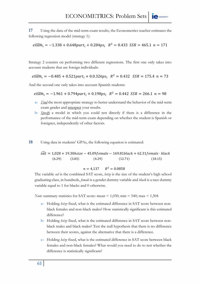
ECONOMETRICS: Problem Sets
61
17 Using the data of the mid-term exam results, the Econometrics teacher estimates the
following regression model (strategy 1):
𝑒𝑥𝑎𝑚𝑖 = −1.338 + 0.648𝑝𝑎𝑟𝑡𝑖 + 0.284𝑝𝑠𝑖 𝑅2 = 0.433 𝑆𝑆𝑅 = 465.1 𝑛 = 171
Strategy 2 consists on performing two different regressions. The first one only takes into
account students that are foreign individuals:
𝑒𝑥𝑎𝑚𝑖 = −0.485 + 0.521𝑝𝑎𝑟𝑡𝑖 + 0.0.326𝑝𝑠𝑖 𝑅2 = 0.432 𝑆𝑆𝑅 = 175.4 𝑛 = 73
And the second one only takes into account Spanish students:
𝑒𝑥𝑎𝑚𝑖 = −1.961 + 0.794𝑝𝑎𝑟𝑡𝑖 + 0.198𝑝𝑠𝑖 𝑅2 = 0.442 𝑆𝑆𝑅 = 266.1 𝑛 = 98
a- Find the most appropriate strategy to better understand the behavior of the mid-term
exam grades and interpret your results.
b- Specify a model in which you could test directly if there is a difference in the
performance of the mid-term exam depending on whether the student is Spanish or
foreigner, independently of other factors.
18 Using data in students’ GPAs, the following equation is estimated:
𝑠𝑎�� = 1,028 + 19.30ℎ𝑠𝑖𝑧𝑒 − 45.09𝑓𝑒𝑚𝑎𝑙𝑒 − 169.81𝑏𝑙𝑎𝑐𝑘 + 62.31𝑓𝑒𝑚𝑎𝑙𝑒 ∙ 𝑏𝑙𝑎𝑐𝑘
(6.29) (3.83) (4.29) (12.71) (18.15)
𝑛 = 4,137 𝑅2 = 0.0858
The variable sat is the combined SAT score, hsize is the size of the student’s high school
graduating class, in hundreds, female is a gender dummy variable and black is a race dummy
variable equal to 1 for blacks and 0 otherwise.
Note: summary statistics for SAT score: mean = 1,030; min = 540; max = 1,504
a- Holding hsize fixed, what is the estimated difference in SAT score between non-
black females and non-black males? How statistically significant is this estimated
difference?
b- Holding hsize fixed, what is the estimated difference in SAT score between non-
black males and black males? Test the null hypothesis that there is no difference
between their scores, against the alternative that there is a difference.
c- Holding hsize fixed, what is the estimated difference in SAT score between black
females and non-black females? What would you need to do to test whether the
difference is statistically significant?

ECONOMETRICS: Problem Sets
62
19 We have the following estimated regression model:
log (𝑤𝑖) = 1.6 − 0.32𝑓𝑒𝑚𝑖 + 0.16log (𝑠𝑖𝑧𝑒𝑖) + 0.05𝑒𝑑𝑢𝑖 𝑅2 = 0.31 𝑆𝑆𝑅 = 359
(0.02) (0.02) (0.02) (0.002)
Such that 𝑤𝑖 measures salaries in thousand dollars for each of our 2,000 sampled individuals,
𝑒𝑑𝑢𝑖 measures education in years, 𝑓𝑒𝑚𝑖 is a gender dummy variable with a value of 1 if the
individual i is a female, and size is a variable measuring the number of workers working in
the company.
a- Interpret the above estimation results.
b- Are gender and company size categorical factors statistically significant?
We estimate an alternative model changing the previous specification such that:
log (𝑤𝑖) = 1.6 − 0.26𝑓𝑒𝑚𝑖 + 0.18log (𝑠𝑖𝑧𝑒𝑖) + 0.05𝑒𝑑𝑢𝑖 − 0.16𝑓𝑒𝑚𝑖 ∗ log (𝑠𝑖𝑧𝑒𝑖)
𝑅2 = 0.32 𝑆𝑆𝑅 = 341
c- Do small companies discriminate against women more or less than larger firms? Is
the discrimination statistically significant?
20 The following model is regressed using data in quarterly form from 1990 to 2005 (64
observations) for Malaysian stock prices against output knowing that there was an economic
crisis in 1997.
𝑌𝑡 = 𝛽0 + 𝛽1𝑋𝑡 + 𝑈𝑡
The first regression using all the data produced a SSR of 0.56. Then, two regressions were
run. The first one on a subsample of the data from 1990-1997, giving a SSR of 0.23. The
second one was on the simple from 1998 to 2005, producing a SSR of 0.17. Test whether the
crisis in 1997 produced a significant shock in the behavior of Malaysian stock prices.
21 We have the following estimated regression model:
𝑦�� = 186.4 + 2.33𝑥𝑖 − 126𝐷𝑖 − 1.29𝐷𝑖𝑥𝑖 𝑅2 = 0.5055 𝑛 = 34
(45.67) (0.86) (37.01) (1.02)

ECONOMETRICS: Problem Sets
63
Such that 𝑦𝑖 measures annual expenditure on beer in dollars for each of our 34 sampled
individuals, 𝑥𝑖 measures individual annual income in thousand dollars and 𝐷𝑖 is a dummy
variable with a value of 1 if the individual i is a female and 0 if the individual is a male.
a- What will be the difference in consumption between a male and a female with the same
annual income?
b- Test at 1% level the following: there are no differences in beer consumption across
gender.
c- Test at 5% level the following: there are no differences in the marginal propensity to
consume beer respect to income across gender.
22 A regression model was estimated using 350 students to compare performance of
students taking a business statistics course either as a standard 14-weekcourse or as an
intensive 3-week course:
X1 X2 X3 X4 X5 X6 X7
Estimated coeff.
1.417 2.162 0.868 1.0845 0.4694 0.0038 0.0484
Std.Error 0.4568 0.3287 0.4393 0.3766 0.0628 0.0094 0.0776
Where:
Y= score on a standardised test of understanding of statistics after taking the course.
X1= dummy variable taking the value 1 if the 3-week course was taken and 0 if the 14-week
course was taken.
X2= student´s grade point average.
X3= dummy variable taking the value 0 or 1, depending on which of two teachers had taught
the course.
X4= dummy variable taking the value 1 if the student is a male and 0 if female.
X5= score on a standardised test of understanding mathematics before taking the course.
X6= number of semester credit hours the student had completed.
X7= student´s age.
Knowing that the value of the determination coefficient is 0.344, answer the following
questions:
a- Interpret all the beta coefficients.
b- Test the individual significance of X1 at 1% significance level.
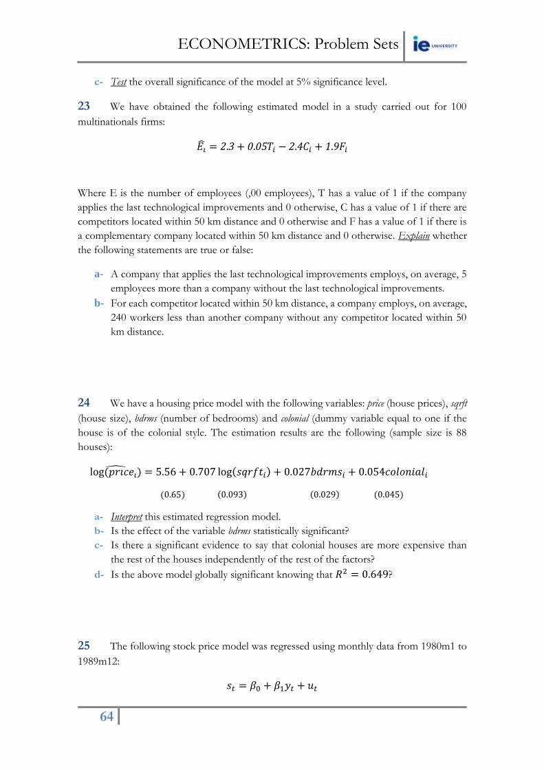
ECONOMETRICS: Problem Sets
64
c- Test the overall significance of the model at 5% significance level.
23 We have obtained the following estimated model in a study carried out for 100
multinationals firms:
𝐸�� = 2.3 + 0.05𝑇𝑖 − 2.4𝐶𝑖 + 1.9𝐹𝑖
Where E is the number of employees (,00 employees), T has a value of 1 if the company
applies the last technological improvements and 0 otherwise, C has a value of 1 if there are
competitors located within 50 km distance and 0 otherwise and F has a value of 1 if there is
a complementary company located within 50 km distance and 0 otherwise. Explain whether
the following statements are true or false:
a- A company that applies the last technological improvements employs, on average, 5
employees more than a company without the last technological improvements.
b- For each competitor located within 50 km distance, a company employs, on average,
240 workers less than another company without any competitor located within 50
km distance.
24 We have a housing price model with the following variables: price (house prices), sqrft
(house size), bdrms (number of bedrooms) and colonial (dummy variable equal to one if the
house is of the colonial style. The estimation results are the following (sample size is 88
houses):
log (𝑝𝑟𝑖𝑐𝑒𝑖) = 5.56 + 0.707 log(𝑠𝑞𝑟𝑓𝑡𝑖) + 0.027𝑏𝑑𝑟𝑚𝑠𝑖 + 0.054𝑐𝑜𝑙𝑜𝑛𝑖𝑎𝑙𝑖
(0.65) (0.093) (0.029) (0.045)
a- Interpret this estimated regression model.
b- Is the effect of the variable bdrms statistically significant?
c- Is there a significant evidence to say that colonial houses are more expensive than
the rest of the houses independently of the rest of the factors?
d- Is the above model globally significant knowing that 𝑅2 = 0.649?
25 The following stock price model was regressed using monthly data from 1980m1 to
1989m12:
𝑠𝑡 = 𝛽0 + 𝛽1𝑦𝑡 + 𝑢𝑡

ECONOMETRICS: Problem Sets
65
It is believed there is a structural break at 1987m11, following a stock market crash. The
regression using all the data produced a SSR of 0.97. Then two further regressions were run
from 1980m1 to 1987m11, which produced a SSR of 0.58 and another regression from
1987m12 to 1989m12 produced a SSR of 0.32.
a- Do you think the stock market crash at 1987m11 was statistically significant?
b- Why are structural breaks a problem for financial econometrics? Give examples of some recent structural breaks.
26 We have the following estimated regression model:
𝑦�� = 100 − 0.8𝑥𝑖 − 0.3𝐷𝑖𝑥𝑖 𝑅2 = 0.47 𝑛 = 55
(27) (0.05) (0.01)
Such that 𝑦𝑖 measures profits in thousand dollars for each of our 55 sampled companies, 𝑥𝑖
measures production costs in thousand dollars and 𝐷𝑖 is a dummy variable with a value of 1
if the company i is a manufacturing firm and 0 if the company is a services firm.
a- Interpret the estimated regression model.
b- Is 𝐷𝑖𝑥𝑖 a significant explanatory variable? Why? Explain your answer.
c- Find the predicted profits for a manufacturing company with 55.000 dollars as
production costs.
27 Let´s consider the following regression model using a sample of annual data from
1970 until 2001 (both included) for the Castilla-León economy:
𝑦�� = 134.6 + 10.89𝑥𝑡 + 21.6𝐷𝑡 + 3.91𝐷𝑡𝑥𝑡 𝑅2 = 0.921
(56.2) (2.06) (3.99) (0.91)
Such that 𝑦𝑡 are annual regional exports, 𝑥𝑡 is the annual exchange rate (pts/$) and 𝐷𝑡 is a
dummy variable equals to 1 if 𝑡 ≤ 1985 and equals to 0 if 𝑡 > 1985 (Spain being a
European Union member).
a- Interpret the above regression model.
b- Test the validity of the additive and multiplicative dummy effects in the above model
at 1% significance level.
c- Test the overall fit of the model at 5% significance level.

ECONOMETRICS: Problem Sets
66
28 The following model was estimated to examine the short run interest rate:
𝑦�� = 5.5 + 0.93𝑥𝑡 − 0.38𝑥𝑡−1 + 0.5𝑦𝑡−1 − 0.05𝐷1𝑡 + 0.08𝐷2𝑡 + 0.06𝐷3𝑡
Such that 𝑥𝑡 is the interest rate for the Treasury bills with a maturity of 90 days and 𝐷𝑖𝑡 are
seasonal dummy variables where 𝑖 corresponds to the first, second and third year quarter
respectively.
Interpret the above estimated regression model.
29 The following wage equations have been estimated using data on workers from
Vietnam:
log(𝑠𝑎𝑙𝑎𝑟𝑦) = 1.25 + 0.15𝑔𝑒𝑛𝑑𝑒𝑟 + 0.02𝑒𝑥𝑝
(0.35) (0.03) (0.004)
log(𝑠𝑎𝑙𝑎𝑟𝑦) = 1.55 + 0.10𝑔𝑒𝑛𝑑𝑒𝑟 + 0.015𝑒𝑥𝑝 − 0.0005𝑔𝑒𝑛𝑑𝑒𝑟 ∗ 𝑒𝑥𝑝
(0.48) (0.05) (0.005) (0.002)
Where salary is measured in US dollars and gender is a dummy variable taking the value of 1
if the worker is a male and 0 if the worker is a female, exp measures the years of work
experience.
a- Why the coefficients associated to gender and experience are lower in the second
than in the first model?
b- What is the estimated average difference between a man´s salary with 5 years work
experience and that of a woman´s with 10 years work experience according to the
first model?
c- What is the estimated average difference between a man´s salary with 5 years work
experience and that of a woman´s with 10 years work experience according to the
second model?
d- Test that the salary difference between men and women does not depend on
experience.
30 To see whether people living in urban areas spend more on fish than people living
in rural areas, we get the following estimation results:

ECONOMETRICS: Problem Sets
67
OLS Estimation results
Dependent: log(expenditure in fish)
Explanatory OLS t-statistic Degrees of Significance t-critical
Variable Coefficient Freedom level
Intercept 6.375 36 0.01 -
log(income) 1.313 5.328 36 0.01 2.719
gender -0.055 -1.378 36 0.01 -2.719
urban 0.143 10.311 36 0.01 2.719
Sample size (n) 40 F-statistic Degrees of Significance F-critical
Freedom level
R-squared 0.750 36 3(n),36(d) 0.01 4.40
Where the dependent variable is expenditure in fish (with log), income is disposable income
(with log), gender is a gender dummy with 1 if male and 0 if female and urban is another
dummy which takes the value 1 if person lives in an urban area. Please, answer the
following three questions:
a- Interpret the above estimations results (only the value of the OLS coefficient for each
of the explanatory variables).
b- Is the variable gender individually significant to explain the behavior of fish
expenditures (at 1% significance level)? Explain.
c- Is the model globally significant at 1% significance level? Explain.
31 A group of researchers in the field of environmental economics has conducted a
survey to investigate patterns of apples’ consumption, both regular and Eco labeled. The
sample contains the responses of 660 individuals. The following information is available:
Variable Description
regq Quantity demanded regular apples, lbs
ecoq Quantity demanded Eco labeled apples, lbs
regp Price of regular apples, pounds
ecop Price of Eco labeled apples, pounds
educ Years of schooling
age Age in years
hhsize Household size
faminc Family income, thousands
male =1 if the individual is a male

ECONOMETRICS: Problem Sets
68
Three different models have been estimated using ecoq as dependent variable. The results
are presented next. (Standard errors in parenthesis)
Model 1 Model 2 Model 3
const 1.965 2.007 1.137 (0.380) (0.387) (0.911) ecop -2.926 -2.962 -2.889 (0.588) (0.592) (0.596) regp 3.029 3.063 3.034 (0.711) (0.714) (0.716) male -0.126 -0.101 (0.221) (0.227) educ 0.034 (0.045) age 0.0008 (0.007) faminc 0.002 (0.003) hhsize 0.057 (0.069)
n 660 660 660 R2 0.036 0.036 0.040 SSR 4051.05 4049.05 4033.81
Note: Set 𝛼 equal to 5% when needed.
a- Interpret the coefficients on the price variables from Model 1 and comment on their
signs and magnitudes. Are regular apples and eco-labeled apples substitute goods?
b- Report the individual t-tests from Model 1. At the individual level, are the price
variables statistically significant?
c- Is there a gender difference in the quantity demand for eco-labeled apples? If so, is
the difference statistically significant? Justify your answer.
d- Compare the goodness of fit between Model 1 and Model 2.
e- Explain with your own words how would you extend Model 3 to allow a different
effect of education on apples’ consumption by gender.
f- Model 3 adds the variables faminc, hhsize, educ and age to the regression from part
(b). Test whether these four variables are jointly significant.

ECONOMETRICS: Problem Sets
69
32 Gathering data for Michigan manufacturing firms in 2010, we obtain the following
estimation results using a log transformation:
OLS Estimation results
Dependent: log(training per employee)
Explanatory OLS t-statistic Degrees of Significance t-critical
Variable Coefficient Freedom level
Intercept 46.67 101 0.01 -
log(sales) 0.987 7.559 101 0.01 2.626
log(employees) -0.555 -10.378 101 0.01 -2.626
grant 0.125 3.111 101 0.01 2.626
Sample size (n) 105 F-statistic Degrees of Significance F-critical
Freedom level
R-squared 0.237 10.456 3(n),101(d) 0.01 3.98
Such that, the dependent variable is hours of training per employee, the variable sales
represents annual sales, employees is the number of employees and grant variable is a dummy
equals to one if the firm received a job training grant for 2010 and zero otherwise. Please,
answer the following three questions:
a- Interpret the above estimations results (only the value of the OLS coefficient for each
of the explanatory variables).
b- Is the variable grant individually significant to explain the dependent variable (at 1%
significance level)? Explain.
c- Is the model globally significant at 1% significance level? Explain.
33 A group of researchers has conducted a survey that contains information on
smoking behavior and other variables for a random sample of 807 single adults from the
United States. The following information is available:
Variable Description
cigs Average number of cigarettes smoked per day
cigprice State cigarette price, cents per pack
educ Years of schooling
age Age in years
income Annual income, dollars
white =1 if the individual is white
restaurn =1 if state restaurant smoking restrictions

ECONOMETRICS: Problem Sets
70
Three different models have been estimated using cigs as dependent variable. The results are
presented next. (Notes: Standard errors in parenthesis; l_ stands for natural logarithm)
Model 1 Model 2 Model 3
const -0.983 -3.765 -2.011 (8.685) (8.898) (8.964)
cigprice -0.048 -0.012 -0.005 (0.102) (0.103) (0.103)
l_income 1.429 1.433 1.891 (0.6793) (0.679) (0.713)
white 0.0009 -0.036 (1.483) (1.479)
restaurn -2.961 -2.949 (1.136) (1.134)
educ -0.377 (0.168)
age -0.045 (0.029)
n 807 807 807 R2 0.005 0.013 0.021 SSR 151052.1 149770.7 148568.0
Note: Set 𝛼 equal to 5% when needed.
a- Interpret the coefficients on the variables from Model 1 and comment on their signs and magnitudes. Is the income effect statistically significant?
b- Interpret the coefficient on the variable restaurn. c- Is there a race difference in the quantity demanded for cigarettes? If so, is the
difference statistically significant? Justify your answer. d- Explain with your own words how you would extend Model 3 to allow a different
effect of education on smoking habits by race. e- Model 3 adds the variables age and educ to the regression from part (b). Test
whether these two variables are jointly significant.
34 An insurance company finds that the probability of having a home insurance or not
can be described by the following linear relationship:
𝑦�� = 0.002𝑖𝑛𝑐𝑖 + 0.004𝑎𝑔𝑒𝑖
Knowing that inc denotes annual income (in thousand Euros) of the individual and age the
age of the individual (in years):
a- Find the probability of having a home insurance for an individual with 400,000 Euros
income and being 30 years old.

ECONOMETRICS: Problem Sets
71
b- Find the increment in the probability of having a home insurance if the individual´s
income increases in 20,000 Euros.
35 A researcher investigates the possibility of a family having home ownership or not.
He uses the following explanatory variables: (1) household income (in thousand Euros), (2)
gender which is a dummy with a 1 if individual is a male and 0 if female, (3) being employed
which is a dummy variable with a 1 if the individual is employed and 0 if unemployed and
(4) age (years). The following logit model is estimated:
𝑦�� = 0.009𝑖𝑛𝑐𝑖 + 0.16𝑔𝑑𝑟𝑖 + 0.02𝑤𝑜𝑟𝑘𝑖 + 0.002𝑎𝑔𝑒𝑖
a- Find the probability of having home ownership for a female individual with 80,000
Euros income, being 46 years old and having a job.
b- What is the difference in the probability of having home ownership between a female
individual and a male individual with the same characteristics.
36 In 1985, neither Florida nor Georgia had laws banning open alcohol containers in
vehicle compartments. By 1990, Florida had passed such a law, but Georgia had not.
a- Suppose you can collect random samples of the driving age population in both states, for 1985 and 1990. Let arrest be a binary variable equal to unity if a person was arrested for drunk driving during the year. Without controlling for any factors, specify a linear probability model that allows you to test whether the open container law reduced the probability of being arrested for drunk driving. Which coeffcient in your model measures the e_ect of the law?
b- Why might you want to control for other factors in the model? What other factors might you want to include? Explain your answer.
37 Suppose that you want to explain the behavior of a binary variable (approve) which is
equal to one if a mortgage loan to an individual was approved. The key explanatory variable
is white, a dummy variable equal to one if the applicant was White. The other applicants in
the dataset are black and hispanic. To test for discrimination in the mortgage loan market, a
linear probability model can be used:
𝑎𝑝𝑝𝑟𝑜𝑣𝑒𝑖 = 𝛽0 + 𝛽1𝑤ℎ𝑖𝑡𝑒𝑖 + 𝑜𝑡ℎ𝑒𝑟𝑓𝑎𝑐𝑡𝑜𝑟𝑠𝑖
a- If there is discrimination against minorities, and the appropriate factors have been
controlled for, what is the sign of 𝛽1? Explain your answer.
b- Regressing approve against white we obtain the following estimation results:

ECONOMETRICS: Problem Sets
72
𝑎𝑝𝑝𝑟𝑜𝑣𝑒𝑖 = 0.707 + 0.201𝑤ℎ𝑖𝑡𝑒𝑖
(0.0182) (0.0198)
𝑛 = 1,989 𝑅2 = 0.048
Interpret the coefficient on White. Is it statistically significant? Is it practically large?
As controls, we add several explanatory variables such as percentage of total income in
housing expenditures, percentage of total income in other obligations, whether the individual
is a male, married and if he/she is unemployed. We re-estimate the model obtaining an
estimate for 𝛽1 = 0.187 and with 𝑠𝑒 = 0.019.
c- Interpret the new beta one coefficient. What happens to the coefficient on white
variable? Is there still evidence of discrimination against non-whites? Explain your
answer.
d- Justify whether the following statement is true or false: “all the fitted values of the
coefficients for the rest of variables in the second model are strictly between zero
and one”

ECONOMETRICS: Problem Sets
73
PS5
Estimation
Problems
COURSE CONTENT
-Chapter 7: Estimation Problems
-Chapter 8: Time Series and Autocorrelation
An econometrician is an expert who will know tomorrow why the things
he predicted yesterday did not happen today.
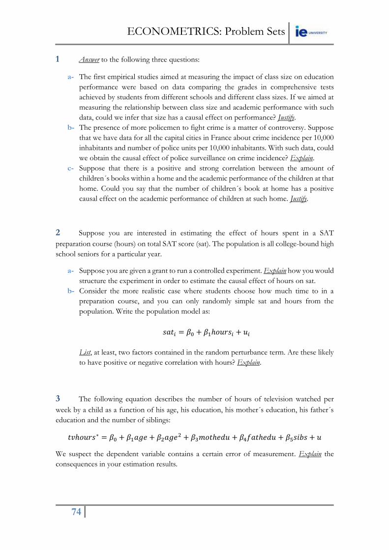
ECONOMETRICS: Problem Sets
74
1 Answer to the following three questions:
a- The first empirical studies aimed at measuring the impact of class size on education
performance were based on data comparing the grades in comprehensive tests
achieved by students from different schools and different class sizes. If we aimed at
measuring the relationship between class size and academic performance with such
data, could we infer that size has a causal effect on performance? Justify.
b- The presence of more policemen to fight crime is a matter of controversy. Suppose
that we have data for all the capital cities in France about crime incidence per 10,000
inhabitants and number of police units per 10,000 inhabitants. With such data, could
we obtain the causal effect of police surveillance on crime incidence? Explain.
c- Suppose that there is a positive and strong correlation between the amount of
children´s books within a home and the academic performance of the children at that
home. Could you say that the number of children´s book at home has a positive
causal effect on the academic performance of children at such home. Justify.
2 Suppose you are interested in estimating the effect of hours spent in a SAT
preparation course (hours) on total SAT score (sat). The population is all college-bound high
school seniors for a particular year.
a- Suppose you are given a grant to run a controlled experiment. Explain how you would
structure the experiment in order to estimate the causal effect of hours on sat.
b- Consider the more realistic case where students choose how much time to in a
preparation course, and you can only randomly simple sat and hours from the
population. Write the population model as:
𝑠𝑎𝑡𝑖 = 𝛽0 + 𝛽1ℎ𝑜𝑢𝑟𝑠𝑖 + 𝑢𝑖
List, at least, two factors contained in the random perturbance term. Are these likely
to have positive or negative correlation with hours? Explain.
3 The following equation describes the number of hours of television watched per
week by a child as a function of his age, his education, his mother´s education, his father´s
education and the number of siblings:
𝑡𝑣ℎ𝑜𝑢𝑟𝑠∗ = 𝛽0 + 𝛽1𝑎𝑔𝑒 + 𝛽2𝑎𝑔𝑒2 + 𝛽3𝑚𝑜𝑡ℎ𝑒𝑑𝑢 + 𝛽4𝑓𝑎𝑡ℎ𝑒𝑑𝑢 + 𝛽5𝑠𝑖𝑏𝑠 + 𝑢
We suspect the dependent variable contains a certain error of measurement. Explain the
consequences in your estimation results.

ECONOMETRICS: Problem Sets
75
4 We have the following variables:
Y: Food expenditure in USA.
X: Family income.
P: Price index.
Two different regressions are estimated with the following estimation results (standard errors
are in brackets and sample size is 500):
Regression Coefficient for
X Coefficient for
P Adjusted Determination
coefficient
Y / P 2.462 0.614
(0.407) Y / X; P 0.112 -0.739 0.978
(0.003) (0.114)
Find and discuss the specifation error the first model is suffering. Explain it using the estimation
results of the above table.
5 There is an econometric study at IE University, which relates the average grade in
Econometrics with the time students employ in different activities during the week. Some
students are asked about how many hours they employ in four different activities: study,
sleep, work and leisure. Any activity must be included in one of these four categories such
that the time spent in the four activities is 168 hours for each student.
The model is the following:
𝐴𝐺𝐸 = 𝛽0 + 𝛽1𝑠𝑡𝑢𝑑𝑦 + 𝛽2𝑠𝑙𝑒𝑒𝑝 + 𝛽3𝑤𝑜𝑟𝑘 + 𝛽4𝑙𝑒𝑖𝑠𝑢𝑟𝑒 + 𝑢
a- Find the assumption that does not hold in this model and explain why.
b- How would you rewrite the model in order to solve the problem?

ECONOMETRICS: Problem Sets
76
6 We have estimated a SLRM explaining office rental prices in the city of Madrid (Y)
with the information contained in distance to the city center (X). The following two graphs:
Figure 1(Y versus X) and Figure 2 (residuals versus fitted values of Y) are related to the above
model.
Figure 1 Figure 2
a- Discus according to the two graphs if the model may suffer a non-linearity problem
b- Provide an economic reason explaining the possible non-linearity in the above
relationship.
c- How should Figure 2 be if the relationship between office rental prices and distance
was a linear relationship?
7 The following table shows two different samples with two explanatory variables each
of them in order to study the behavior of Y (dependent variable):
Sample 1 Sample 2
Observation Y X1 X2 Z1 Z2
1 1 2 4 2 4
2 4 6 12 6 12
3 2 4 11 4 8
a- Can you detect a multicollinearity problem in any of the two samples?
b- If yes, please explain the consequences in your OLS estimations in each sample.
c- If yes, please explain the strategies that you would use in order to solve the problem
in each sample.

ECONOMETRICS: Problem Sets
77
8 Consider the regression of country level GDP per capita on percentage urban
population in several countries (1995) obtaining a determination coefficient of 0.457 and
obtaining the following graph when plotting the data (Figure 1):
Figure 1: GDPpc versus % urban pop
a- Can you detect a non-linear relationship between the two variables? Why?
b- Can you explain solutions to be implemented in order to solve the non-linearity
problem?
Suppose now that we estimate the same model but using a semilog transformation obtaining
the following estimation results:
log (𝐺𝐷𝑃𝑝𝑐)𝑖 = 4.631 + 0.052𝑢𝑟𝑏𝑎𝑛𝑖 𝑅
2 = 0.549
and obtaining Figure 2 when plotting the data:
Figure 2: logGDPpc versus % urban pop.
c- Compare the determination coefficients and the graphs between the two models. Do
you think the semilog transformation might be a good solution for the nonlinearity
problem? Explain your answer.

ECONOMETRICS: Problem Sets
78
9 We have data for a sample of high schools in Vietnam where the variable math
denotes the percentage of students who passed a math test. We want to estimate the effect
that spending per student has on the outcomes of this test and propose the following model:
𝑚𝑎𝑡ℎ = 𝛽0 + 𝛽1 log(𝑠𝑝𝑒𝑛𝑑) + 𝛽2 log(𝑒𝑛𝑟𝑜𝑙𝑙) + 𝛽3𝑝𝑜𝑣𝑒𝑟𝑡𝑦 + 𝑢
Where poverty describes the percentage of students living below the poverty line, spend denotes
spending per student and enroll is the number of students enrolled in the high school.
a- We do not have data for poverty variable but the variable lnchprg describes the
percentage of students eligible for a programme subsidising school lunches. Why is
this variable a sensible proxy variable for poverty?
b- The table below shows the OLS estimates with and without the inclusion of lnchprg
as an explanatory variable:
Explanatory variables (1) (2)
log(spend) 11.13 7.75
(3.30) (3.04)
log(enroll) 0.022 -1.26
(0.615) (0.58)
lnchprg - -0.324
(0.036)
intercept -69.24 -23.14
(26.74) (24.99)
n 408 408
Determination coefficient 0.0293 0.1893
Explain why the effect of spending and enrol are greater in the first model than in
the second one? What about if we compare standard errors between the two models?
c- What conclusions can you derive when comparing both models?
10 We want to estimate a regression model explaining the behavior of property prices
in the city of Barcelona in 2015 (cross sectional analysis). We are provided with a dataset
containing information about property, neighborhood and buyer´s characteristics that can
be used as explanatory variables. The following table describes those variables:

ECONOMETRICS: Problem Sets
79
VARIABLE
NAME
DESCRIPTION
advance Loan amount when buying the property
age Age of property
bathroom Number of bathroms
bedroom Number of bedrooms
buyage Age of main buyer
chnone No central heating (dummy)
dcitycenter Distance to city center (km)
floorm2 Floor area of dwelling (m2)
ftbuyer First time buyer (dummy)
lagood
labad
Dwelling is in neighborhood with higher-status social housing
Dwelling is in neighborhood with lower-status social housing
pflat Flat/maisonnette dwelling (dummy)
psemi
pdetach
Semi-detached dwelling (dummy)
Detached dwelling (dummy)
pterrace Terraced dwelling (dummy)
a- In order to avoid specification errors, which variables would you keep in your analysis
according to practical significance? Justify your choices.
b- Explain, the process you would follow in order to specify your final model and to
choose the final variables in your model.
c- Explain the difference between practical and statistical significance.
11 We have the following information for the annual growth rates (%) in different
countries about stock prices (Y) and in consumer prices (X):

ECONOMETRICS: Problem Sets
80
Country Stock prices
(Y) Consumer prices (X) Predicted
Y Estimation Residuals
Australia 5 4.3 Austria 11.1 4.6 Belgium 3.2 2.4 Canada 7.9 2.4 Denmark 3.8 4.2 Finland 11.1 5.5 France 9.9 4.7 Germany 13.5 2.2 India 1.5 4 Ireland 6.4 4 Israel 8.9 8.4 Italy 8.1 3.3 Japan 13.5 4.7 Mexico 4.7 5.2 Netherlands 7.5 3.6 New Zealand 4.7 3.6 Sweden 8 4 UK 7.5 3.9 USA 9 2.1
Knowing that: 𝑦�� = 6.83 + 0.201𝑥𝑖
Answer to the following questions:
a- Complete the missing values in the above table.
b- Show both graphically and formally if the above data suffers from an outlier problem.
c- If the answer to b is positive, please explain any strategy you would perform in order
to solve the problem.
12 Imagine that you are interested in analyzing the determinants of infant mortality rates
worldwide. Using the Development Reports from the World Bank in 2013, you get the
following information for 248 countries:
IMR Infant Mortality rate - is the number of deaths of infants per 1,000 live births.
GDP GDP per capita (constant 2005 US$)
Source: World Bank Development Reports, 2013.
And construct the following figure:

ECONOMETRICS: Problem Sets
81
a- Have a look at the graph above, why Angola and Guinea might be considered as
outliers in this regression model? Comment on the implications of the inclusion of
these two countries in the analysis.
b- Angola presents one of the highest infant mortality rates in this sample (103 per 1,000
live births). Compute the residual for this country given that our model predicts for
Angola an infant mortality rate of 28.6 per 1,000 live births.
c- Knowing that the standard deviation of the estimation residuals (using all the
observations) is 26.22, is Angola a significant outlier?
d- What about Guinea? Note that the estimation residual associated to Guinea
observation is 52.
13 We have representative data for 30 years old for the US. Levine, Gustafson and
Velenchik (1997) estimated a wage equation using the following variables:
Y = log(wage)
F = a dummy variable that takes a value of 1 for smokers and 0, otherwise
ED = years of education
Two specifications are considered:

ECONOMETRICS: Problem Sets
82
MODEL 1: Y = -0.176F omitting education
(se=0.031)
Coefficient of determination = 0.35
MODEL 2: Y = -0.080F + 0.070ED including education
(se=0.021) (se=0.0004)
Coefficient of determination = 0.68
Compare the two fitted models and explain what happens when we omit one relevant variable
(in this case, years of education).
14 Consider the following regression model with 41 observations (countries):
log(𝑦𝑖) = 𝛽0 + 𝛽1 log(𝑥1𝑖) + 𝛽2 log(𝑥2𝑖) + 𝑢𝑖
Such that the dependent variable is the ratio of trade taxes (imports and export taxes) to total
government revenues, the first explanatory variable is the ratio of exports plus imports to
GDP and the second explanatory variable is GDP per capita. We estimate this model using
OLS and obtain the residuals of the above regression. Then we do the following auxiliary
regression:
log(𝑦𝑖) = −5.8 + 2.5 log(𝑥1𝑖) + 0.69 log(𝑥2𝑖) − 0.4[log(𝑥1𝑖)]2
−0.04[log(𝑥2𝑖)]2 + 0.002 log(𝑥1𝑖) log (𝑥2𝑖)
Knowing that the determination coefficient for the auxiliary equation is 0.1148. Could you
compute the White statistic? What is your conclusion about heteroscedasticity in your regression
model?
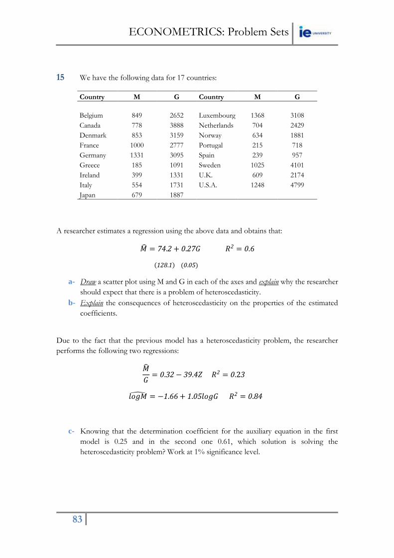
ECONOMETRICS: Problem Sets
83
15 We have the following data for 17 countries:
Country M G Country M G
Belgium 849 2652 Luxembourg 1368 3108
Canada 778 3888 Netherlands 704 2429
Denmark 853 3159 Norway 634 1881
France 1000 2777 Portugal 215 718
Germany 1331 3095 Spain 239 957
Greece 185 1091 Sweden 1025 4101
Ireland 399 1331 U.K. 609 2174
Italy 554 1731 U.S.A. 1248 4799
Japan 679 1887
A researcher estimates a regression using the above data and obtains that:
�� = 74.2 + 0.27𝐺 𝑅2 = 0.6
(128.1) (0.05)
a- Draw a scatter plot using M and G in each of the axes and explain why the researcher
should expect that there is a problem of heteroscedasticity.
b- Explain the consequences of heteroscedasticity on the properties of the estimated
coefficients.
Due to the fact that the previous model has a heteroscedasticity problem, the researcher
performs the following two regressions:
𝑀
𝐺
= 0.32 − 39.4𝑍 𝑅2 = 0.23
𝑙𝑜𝑔�� = −1.66 + 1.05𝑙𝑜𝑔𝐺 𝑅2 = 0.84
c- Knowing that the determination coefficient for the auxiliary equation in the first
model is 0.25 and in the second one 0.61, which solution is solving the
heteroscedasticity problem? Work at 1% significance level.

ECONOMETRICS: Problem Sets
84
16 Explain the estimation problem that can be found in the following graph (predicted
values of the dependent variable versus estimation residuals):
17 Consider the following regression model with 41 observations:
log(𝑌𝑖) = 𝛽0 + 𝛽1𝑋1 + 𝛽2𝑋2 + 𝑢𝑖
where Y = ratio of trade taxes (import and export taxes) to total government revenue, X1 =
ratio of the sum of exports plus imports to GNP, and X2 = GNP per capita.
By computing the auxiliary regression, we compute its determination coefficient obtaining
a value of 0.1148.
a- Write the theoretical specification of the auxiliary regression given the above model.
b- Test for heteroscedasticity at 5% significance level.
18 We have the following regression model explaining the behavior of R&D
expenditures in 18 sectors of the economy using sales and profits as independent factors:
𝑅��𝑖 = −139.392 + 0.012𝑠𝑎𝑙𝑒𝑠𝑖 + 0.239𝑝𝑟𝑜𝑓𝑖𝑡𝑠𝑖

ECONOMETRICS: Problem Sets
85
a- Look at the following three graphs and explain why we should expect
heteroscedasticity in the above regression model.
b- The following auxiliary regression was estimated:
𝑒𝑖2 = 695,1942 + 1,349.7𝑠𝑎𝑙𝑒𝑠𝑖 − 19,656.9𝑝𝑟𝑜𝑓𝑖𝑡𝑠𝑖 − 0.0027𝑠𝑎𝑙𝑒𝑠𝑖
2
−0.1163𝑝𝑟𝑜𝑓𝑖𝑡𝑠𝑖2 + 0.0501𝑠𝑎𝑙𝑒𝑠𝑖 ∗ 𝑝𝑟𝑜𝑓𝑖𝑡𝑠𝑖 𝑅𝑠
2 = 0.889
Test for heteroscedasticity at 1% significance level.
19 We want to estimate a demand function for daily cigarette consumption. Since most
people do not smoke, the dependent variable, cigs, is zero for most observations. The
equation to be estimated uses the following explanatory variables: income (annual income in

ECONOMETRICS: Problem Sets
86
Dollars), cigprc (state cigarette price cents per pack), educ (years of schooling), age (in years)
and restaurn (dummy equal to one if there is state restaurant smoking restrictions). Using a
simple of 807 individuals we obtain the following estimation results:
𝑐𝑖𝑔𝑠�� = 0.375 + 0.00005𝑖𝑛𝑐𝑜𝑚𝑒𝑖 + 0.00053𝑐𝑖𝑔𝑝𝑟𝑐𝑖 − 0.494𝑒𝑑𝑢𝑐𝑖 + 0.784𝑎𝑔𝑒𝑖
(6.874) (0.0000569) (0.1008) (0.168) (0.159)
−0.0091𝑎𝑔𝑒𝑖2 − 2.845𝑟𝑒𝑠𝑡𝑎𝑢𝑟𝑛𝑖
(0.0017) (1.112)
𝑛 = 807 𝑅2 = 0.052
a- Interpret the above estimation results. Are they realistic?
b- Test the individual significance of income and cigprc variables and explain.
c- Do policies, such as restaurant smoking restrictions, affect in a significant and
expected way on smoking habits?
We plot actual (reds) and fitted (blues) values of cigs variable by observation number
obtaining the following graph:

ECONOMETRICS: Problem Sets
87
d- Looking at the actual values, do you think this model is linear? Why?
e- Some of the fitted values are negative values. Do you think this is realistic?
f- Do the errors underlying the above equation contain heteroscedasticity? Test for
heteroscedasticity at 1% significance level knowing that the determination coefficient
of the auxiliary regression is equal to 0.0649. Show both the F-test and the Chi-
squared tests. Are your two results consistent?
20 We use data about 88 properties to test for heteroscedasticity in a simple housing
price equation using the following three independent factors: lotsize (size of lot in square
feet), sqrft (size of house in square feet) and bdrns (number of bedrooms). We estimate two
different models: Model 1, which is the linear model, and model 2, which is the log model.
The table below shows estimation results for both models.
a- Interpret the coefficient associated to bdrms in both models.
b- Specify the auxiliary regression to be able to perform the White test in Model 1 and
explain.
c- Which model is homoscedastic at 1% significant level? Explain your answer.
OLS Estimation Results
Variable Model 1 Model 2
constant -21.77 5.61
(29.48) (0.65)
lotsize 0.00207
(0.00064) sqrft 0.123
(0.013) bdrms 13.85 0.037
(9.01) (0.028)
log(lotsize) 0.168
(0.038)
log(sqrft) 0.71
(0.093)
n 88 88
R squared 0.672 0.643
R squared auxiliary regression 0.383 0.108

ECONOMETRICS: Problem Sets
88
21 Answer to the following five questions:
a- Explain the main differences between the trend and the irregular component in a
time series.
b- Explain the main differences between a cyclical and a seasonal component in a time
series.
c- Explain an econometric tool to take into account seasonal components in a time
series.
d- Explain one possible econometric tool to detect irregular components in a time series.
e- Explain how the trend component can be identified in a SLRM.
22 The general fertility rate (gfr) is the number of children born to every 1,000 women
of childbearing age. For years 1913 through 1984, the equation:
𝑔𝑓𝑟𝑡 = 𝛽0 + 𝛽1𝑝𝑒𝑡 + 𝛽2𝑤𝑤2𝑡 + 𝛽3𝑝𝑖𝑙𝑙𝑡 + 𝑢𝑡
explains gfr in term of the average real dollar value of the personal tax exemption (pe) and
two dummy variables. The variable ww2 takes on the value unity during the years 1941
through 1945, when the United States was involved in World War II. The variable pill is
unity from 1963 on, when the birth control pill was made available for contraception. Using
a dataset, the following estimation results were obtained:
OLS Estimation Results
Variable Model 1 Model 2
constant 98.68 95.87
(3.21) (3.28)
ww2 -24.24 -22.13
(7.46) (10.73)
pill -31.59 -31.30
(4.08) (3.98)
pe(t) 0.083 0.073
(0.03) (0.126)
pe(t-1) -0.0058
(0.1557)
pe(t-2) 0.034
(0.126)
n 72 70
SSR 14,664.27 13,032.64
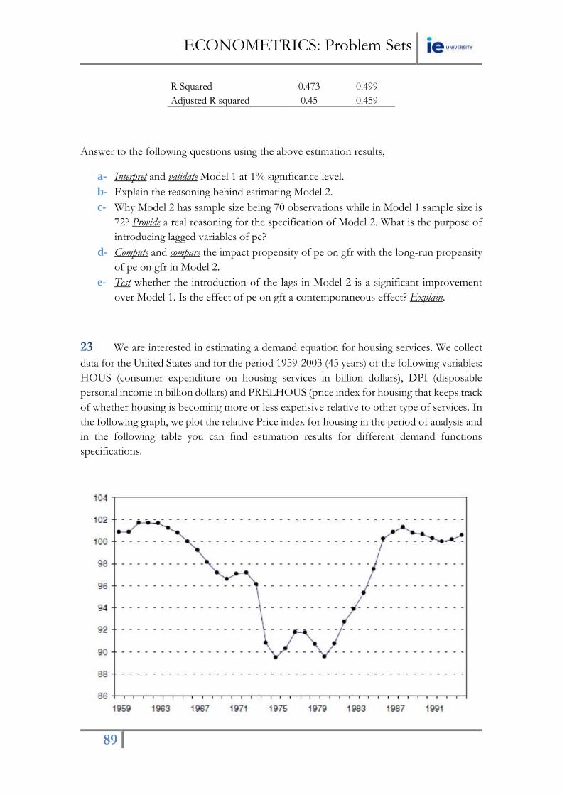
ECONOMETRICS: Problem Sets
89
R Squared 0.473 0.499
Adjusted R squared 0.45 0.459
Answer to the following questions using the above estimation results,
a- Interpret and validate Model 1 at 1% significance level.
b- Explain the reasoning behind estimating Model 2.
c- Why Model 2 has sample size being 70 observations while in Model 1 sample size is
72? Provide a real reasoning for the specification of Model 2. What is the purpose of
introducing lagged variables of pe?
d- Compute and compare the impact propensity of pe on gfr with the long-run propensity
of pe on gfr in Model 2.
e- Test whether the introduction of the lags in Model 2 is a significant improvement
over Model 1. Is the effect of pe on gft a contemporaneous effect? Explain.
23 We are interested in estimating a demand equation for housing services. We collect
data for the United States and for the period 1959-2003 (45 years) of the following variables:
HOUS (consumer expenditure on housing services in billion dollars), DPI (disposable
personal income in billion dollars) and PRELHOUS (price index for housing that keeps track
of whether housing is becoming more or less expensive relative to other type of services. In
the following graph, we plot the relative Price index for housing in the period of analysis and
in the following table you can find estimation results for different demand functions
specifications.

ECONOMETRICS: Problem Sets
90
OLS Estimation Results
Dependent variable: log(HOUS)
Variable Model 1 Model 2 Model 3
log(DPI) 1.03 0.33 0.25
(0.01) (0.15) (0.14) log(DPI)(-1) 0.58 0.20
(0.15) (0.20) log(DPI)(-2) 0.49
(0.13) log(GPRHOU) -0.48 -0.09 -0.28
(0.04) (0.17) (0.17) log(GPRHOU)(-1) -0.36 0.23
(0.17) (0.30) log(GPRHOU)(-2) -0.38 (0.18)
T 36 35 34 Adjusted R squared 0.998 0.999 0.999
a- Interpret the graph above.
b- Interpret estimation results of Model 1.
c- What is the impact elasticity of HOUS respect to DPI in Model 2? What about in
Model 3? Compare them.
d- What is the long-run elasticity of HOUS respect to GPRHOU in Model 2? What
about in Model 3? Compare them.
e- Compare the long-run elasticities of HOUS respect to DPI and respect to GPRHOU
in Model 3.
f- Explain the strategy and econometric tools you would use in order to choose the best
specification among the three models above.
24 A student (so-called A) has information about 30 observations for two variables, X
and Y. He is told that Y depends on X and on a random term such that:
𝑦𝑡 = 𝛽0 + 𝛽1𝑥𝑡 + 𝑢𝑡
He is asked to estimate 𝛽1. He does not know that the true value of 𝛽1 is 5, and he performs
the following experiments:

ECONOMETRICS: Problem Sets
91
1) He uses first OLS and estimate 𝛽1 obtaining the following results: ��1=4.64;
se(��1)=1.30.
2) Next, he is told that the random term follows a first order autoregressive model such
that:
𝑒�� = 0.7𝑒𝑡−1 + 휀𝑡
Where 휀𝑡 satisfies G-M conditions.
Student A defines the following:
𝑦𝑡∗ = 𝑦𝑡 − 0.7𝑦𝑡−1
𝑥𝑡∗ = 𝑥𝑡 − 0.7𝑥𝑡−1
And he performs the regression using 𝑦𝑡∗ as the dependent variables and 𝑥𝑡
∗ as the
explanatory variable, obtaining the following results: ��1=5.14; se(��1)=0.75.
Nine different students (so-called B, C, D…J) perform the same two experiments but with
different random terms. The results are shown in the following table:
Student Exp. 1 Exp. 2
��1 se(��1) ��1 se(��1)
A 4.64 1.3 5.14 0.75
B 4.56 1.57 4.96 0.87
C 6.54 1.77 5.57 0.98
D 5.19 0.9 5.49 0.63
E 5.81 1.3 5.37 0.77
F 5.24 1.22 4.92 0.65
G 4.27 1.1 4.19 0.61
H 5.26 0.97 4.7 0.71
I 6.8 1.55 6.17 0.76
J 3.83 1.72 5.33 0.82
a- Compare and explain why students should not be satisfied with the results obtained in
the first experiment.
b- Explain why students should be satisfied with the results in the second experiment
when they were told that:
𝑒�� = 0.7𝑒𝑡−1 + 휀𝑡

ECONOMETRICS: Problem Sets
92
c- Test for autocorrelation at 1% significance level knowing that the standard error
associated to the 0.7 coefficient of the AR(1) process is equal to 0.11. Explain the
type of autocorrelation the model is suffering.
25 Are changes in consumer prices over time related to changes in manufacturing
capacity utilization, changes in the money supply, and unemployment rates? We have
information about the following variables for the 40 recent years. The variables to be
investigated are:
ChCPI = change in the Consumer Price Index (all items)
CapUtil = change in the manufacturing capacity utilization rate
ChgM1 = change in the M1 component of the money supply
ChgM2 = change in the M2 component of the money supply
Unem = unemployment rate (percent)
a- Validate the model both individually and globally at 1% significance level.
b- You are told the structure of the error terms in the above model follows the following
structure:
𝑒�� = −0.88𝑒𝑡−1 + 휀𝑡
(0.22)

ECONOMETRICS: Problem Sets
93
Test for autocorrelation at 5% significance level and explain your answer and the type
of autocorrelation the model is suffering.
26 A money demand function is defined as follows:
𝑙𝑜𝑔(𝑀1𝑡) = 𝛼 + 𝛽1𝑙𝑜𝑔(𝐺𝐷𝑃𝑡) + 𝛽2𝑅𝑆𝑡 + 𝛽3𝑃𝑅𝑡 + 𝑢𝑡
Where M1 is the narrow money supply, GDP is real GDP, RS is the interest rate and PR is
the rate of inflation.
The model was estimated using quarterly data for the United states over the period 1952:1-
1992:4 (T=163 observations) and using two different specifications: Model 1 assumes the
model suffers autocorrelation AR(1) and Model 2 assumes the structure in the error terms
following AR(2) process. The following table shows estimation results:
OLS Results
Variable Model 1 Model 2 Model 3
constant -0.56 -1.54 2.33
(0.013) (0.09) (1.01)
log(GDP) 0.997 0.888 0.971
(0.082) (0.091) (0.077)
RS -0.056 -0.044 -0.041
(0.001) (0.001) (0.001)
PR 0.404 0.382 0.377
(0.022) (0.018) (0.021)
e(-1) 0.921 0.765
(0.222) (0.098)
e(-2) -0.329
(0.056)
T 163 162 161
SSR 1,796.49 792.54 716.72
Adjusted R squared 0.738 0.739 0.812
Note that the dependent variable in Model 1 is log(M1) and the dependent variable in Models
2 and 3 is the estimation residuals of Model 1.
a- Test for autocorrelation using Model 2 at 1 % significance level.
b- Test for autocorrelation using Model 3 at 1% significance level.
c- Explain the conclusion you arrive at with regard to the serial correlation in our money
demand function.

ECONOMETRICS: Problem Sets
94
27 Consider the following dynamic linear regression model:
𝑦�� = 0.05 + 0.95𝑦𝑡−1 + 0.97𝑥𝑡 𝑇 = 120 𝑅2 = 0.95
(0.01) (0.05) (0.11)
Knowing that the error term follows a second order autoregressive structure:
a- Specify the auxiliary regression to be estimated in order to be able to test for
autocorrelation.
b- Knowing that the LM statistic (Breusch-Godfrey) is 12.30, compute the determination
coefficient of the auxiliary regression.
c- Test for autocorrelation at 1% significance level.
28 Explain the following two graphs: (a) upper two graphs and (b) lower two graphs in
terms of autocorrelation.

ECONOMETRICS: Problem Sets
95
29 We want to analyze quarterly new car sales on price, income, unemployment and
population over 64 quarters and we obtain the following estimation results:
𝑁𝐶𝑆�� = 25,531 + 50.116𝑃𝑅𝐶𝑡 + 630.491𝐼𝑁𝐶𝑡 − 41.812𝑈𝑁𝑡 − 150.679𝑃𝑂𝑃𝑡
𝑇 = 64 𝑅2 = 0.441
However, you are told this model is naïve since you can allow for serial correlation of fourth
order. Please, answer the following two questions:
a- Specify the auxiliary regression to be estimated in order to be able to test for
autocorrelation.
b- Knowing that the LM statistic (Breusch-Godfrey) is 26.486, test for autocorrelation
at 1% significance level.
30 Answer to the following multiple-choice questions about estimation problems:
A- Autocorrelation refers to a situation in which:
a- Successive error terms derived from the application of regression analysis to time
series data are correlated.
b- There is a high degree of correlation between two or more of the independent
variables included in a multiple regression model.
c- The dependent variable is highly correlated with the independent variable(s) in a
regression analysis.
d- The application of a multiple regression model yields estimates that are nonlinear in
form.
B- A situation in which measures of two or more variables are statistically related but
are not in fact causally linked because the statistical relationship is caused by a third
omitted variable is called:
a- Partial correlation
b- Linear correlation
c- Spurious correlation
d- Marginal correlation

ECONOMETRICS: Problem Sets
96
C- Step-wise regression is the most widely used search procedure of developing the
……….. regression model without examining all possible models.
a- worst
b- best
c- medium
d- least
D- If there is measurement error in both dependent and explanatory variables of your
simple linear regression model, then
a- OLS is unbiased but inefficient.
b- OLS is unbiased but inconsistent.
c- OLS is biased and inefficient.
d- OLS is biased but efficient.
E- A non-formal way to detect a non-linearity problem is plotting your model fitted
values versus the
a- Values of your independent variables
b- Values of your explanatory variables
c- Model residuals
d- Model predictions
F- Multicollinearity refers to a situation in which
a- The dependent variable is highly correlated with the explanatory variables included
in the regression model.
b- There is a high degree of correlation between the explanatory variables included in a
multiple regression model.
c- The application of a multiple regression model yields estimates that are nonlinear
form.
d- None of the above.
G- If your dataset has heteroscedasticity, but you completely ignore the problem and
use OLS, you will
a- Get biased estimates of the parameters.

ECONOMETRICS: Problem Sets
97
b- Get parameter standard errors that could be either too large or too small.
c- Get t-statistics that make you too optimistic about your parameters being statistically
different from zero.
d- Get t-statistics that make you too pessimistic about your parameters being statistically
different from zero.
H- A useful graphical method for detecting the presence of heteroscedasticity is
a- Plot 𝑦 against each 𝑥 variable in turn
b- Plot the residuals from a preliminary regression against the 𝑥 variables, each in turn
c- Plot the squared residuals from a preliminary regression against the 𝑥 variables, each
in turn
d- Plot the logarithm of the squared residuals from a preliminary regression against the
𝑥 variables, each in turn