i

ECONOMETRIC MODELLING OF IMPORT DEMAND ANDEXPORT SUPPLY IN TURKEY

The Institute of Economics and Social SciencesOf

Bilkent University

by

SAYGIN ÇEVİK

In Partial Fulfillment of the Requirements for the Degreeof

MASTER OF ECONOMICS

in

THE DEPARTMENT OF ECONOMICSBILKENT UNIVERSITY

ANKARA

July 2001

ii

I certify that I have read this thesis and have found that it is fully adequate, inscope and in quality, as a thesis for the degree of Master of Economics.

---------------------------------------------Assist. Prof. Kıvılcım Metin

Supervisor

I certify that I have read this thesis and have found that it is fully adequate, inscope and in quality, as a thesis for the degree of Master of Economics.

---------------------------------------------Assist. Prof. Fatma TaşkınExamining Comitee Member

I certify that I have read this thesis and have found that it is fully adequate, inscope and in quality, as a thesis for the degree of Master of Economics.

---------------------------------------------Assist. Prof. Nazmi DemirExamining Comitee Member

Approval of the Institute of Economics and Social Sciences

---------------------------------------------Prof. Kürşat AydoğanDirector

iii

ABSTRACT

ECONOMETRIC MODELLING OF IMPORT DEMAND

AND EXPORT SUPPLY IN TURKEY

Çevik, Saygın

Master of Economics

Supervisor: Assist. Prof. Kıvılcım Metin

July, 2001

In this thesis, I estimate the export supply and import demand equations for

Turkey using quarterly data over the period 1989-2000. Unlike the previous

studies done for Turkey, in this study the sub-items of the total import demand,

namely, intermediate, capital and consumption goods import demand equations are

estimated. In empirical analysis, first the cointegration is tested by using two

different approaches: Engle-Granger (1987) and Johansen (1991) approach. After

finding long-run relationships, error correction models are specified and estimated

for export supply and import demand equations respectively. The main conclusion

that emerges from empirical results is that foreign trade developments in Turkey

are highly dependent on the economic activity and the effects of exchange rate

policy on imports and exports appear to be fairly limited.

Key Words: Import, Export, Cointegration, Error Correction Model

iv

ÖZET

TÜRKİYE’DEKİ İHRACAT ARZI VE İTHALAT TALEBİ

DAVRANIŞLARININ EKONOMETRİK OLARAK İNCELENMESİ

Çevik, Saygın

Yüksek Lisans, İktisat Bölümü

Tez Yöneticisi: Yrd. Doç. Kıvılcım Metin

Temmuz, 2001

Bu tez ihracat arz ve ithalat talep denklemlerini, 1989-2000 tarihleri arasındaki üç

aylık veriler kullanılarak, Türkiye ekonomisi için modellemeye çalışmaktadır. Bu

çalışmanın bugüne kadar Türkiye için yapılmış diğer çalışmalardan farkı ithalat

talebinin hem toplam hem de alt kalemler itibariyle, yani ara malı, sermaye malı ve

tüketim malı ithalat taleplerinin de modellenmesidir. Türkiye’nin uzun dönemli

ihracat ve ithalat analizi için Engle-Granger yöntemi ve Johansen yöntemi olmak

üzere iki ayrı koentegrasyon yöntemi kullanılmıştır. Uzun dönem ilişkileri

bulunduktan sonra, kısa dönem modellemesinde hata düzeltme modelleri

kullanılmıştır. Bu çalışmadaki uygulama sonuçlarından, Türkiye’deki dış ticaret

gelişmelerinin çoğunlukla ülkedeki ekonomik faaliyetlere bağlı olduğu ve döviz

kuru politikalarının ithalat ve ihracat üzerindeki etkisinin sınırlı olduğu sonucuna

varılmıştır.

Anahtar Kelimeler: İthalat, İhracat, Koentegrasyon, Hata Düzeltme Modeli

v

ACKNOWLEDGEMENTS

I am grateful to Asist. Prof. Kıvılcım Metin for her supervision and guidance

throughout the development of this thesis.

I would also like to thank Aslıhan Atabek from the Central Bank of Turkey for her

help and guiding comments.

My foremost thanks go to my family for their endless support and encouragements

throughout all my years of study. And last gratitude is to my dearest Serkan for his

moral support in my hardest days.

vi

TABLE OF CONTENTS

ABSTRACT............................................................................................................iii

ÖZET.......................................................................................................................iv

ACKNOWLEDGEMENTS......................................................................................v

TABLE OF CONTENTS.………….………………………...…………………....vi

CHAPTER 1: INTRODUCTION.................................................................1

CHAPTER 2: HISTORICAL BACKGROUND.…………...……………..5

CHAPTER 3: LITERATURE SURVEY.………………………………...11

CHAPTER 4: ECONOMIC MODELLING.……………………………..17

CHAPTER 5: ECONOMETRIC THEORY...............................................20

5.1 Stationarity…………………........…………………….......20

5.2 Unit Root Test............………………………………….....21

5.3 Cointegration..………………………………...…………..24

5.3.1 Engle-Granger Two-Step Approach………....…....25

5.3.2 Johansen’s VAR Approach...………………….......26

5.4 Error Correction Model........……..…………………….....30

CHAPTER 6: EMPIRICAL RESULTS.....................................................33

6.1 The Data Set..……………………..……………….……...33

6.2 Results of Unit Root Tests....................……..…….……....35

6.3 Results of Cointegration Tests...………………..….….......36

6.3.1 Engle-Granger Cointegration Test Results....…......36

6.3.2 Johansen Cointegration Test Results……….…......38

6.4 Empirical Modelling………………………………………40

CHAPTER 7: CONCLUSION...................................................................46

BIBLIOGRAPHY...................................................................................................51

APPENDIX A.........................................................................................................54

1

CHAPTER 1: INTRODUCTION

Outward oriented growth policies were initiated in Turkey in the 1980s and in the

subsequent years, Turkish economy has gone through various experiences in terms of

foreign trade policies, export performance and growth. As a result of this policy

changes, openness of the economy has increased. Import plus export as a percentage

of GDP has increased from 15 percent in 1980 to 40 percent in 2000.

Expansion and diversification of exports are generally considered necessary for

developing countries to achieve higher and sustainable growth. Over the past few

decades, exports have played a critical role in the economic growth of Turkey and

policies to increase them have often been employed as an instrument to deal with

balance of payment diffuculties. Several sets of policy instruments were used, such

as an export tax rebate system, cash premiums, export credits, exemptions from

import taxes for main inputs and the exchange rate policy. Thus, the importance of

the development of exports for Turkish macroeconomic development is vital.

On the other hand, imports of intermediate and capital goods are critical inputs in the

production of exports in Turkey and the share of intermediate goods and capital

goods imports is approximately 90 percent in total imports. So, the development of

imports is also important for Turkish macroeconomic development.

2

In this respect, the primary purpose of this study is to carry out an econometric

investigation of Turkey’s import and export performance for the period 1989-2000.

In the earlier literature, numerous studies have examined the foreign trade

performance of Turkey. They are generally concentrated on the formulation and

estimation of aggregate export and import functions. However, to our knowledge,

there are no studies reporting estimations of export and import flows at any level of

disaggregation. Since a model for total imports may mask important differences in

the effect of income and price for sub-categories of imports and the imports of

intermediate and capital goods are critical inputs in the production in Turkey, unlike

the previous studies done for Turkey, we also estimate the intermediate, consumption

and capital goods import demand equations.

In the empirical form of the import demand and export supply functions, we follow

“imperfect substitutes” model (Goldstein and Khan (1985)) in which the key

assumption is that neither imports nor exports are perfect substitutes for domestic

goods. In this model, import demand depends positively on domestic income and

negatively on the relative price of imported goods vis-à-vis domestic goods and

export supply depends positively on productive capacity and export prices and

negatively on domestic costs.

There is substantial empirical literature on the estimation of import demand and

export supply functions and the respective income and price elasticities. Deyak, et al.

(1989) studied the structural stability of aggregate and disaggregated US import

demand, Dwyer and Kent (1993) tested the cointegration relationship between import

volumes of Australia and its explanators, Giorgianni and Milesi-Ferrettti (1997)

3

estimated Korean aggregate export and import equations and Beko (1998) estimated

export supply and import demand functions for Slovene economy.

If we look at the studies done for Turkey, Uygur (1997) estimated long and short run

export supply functions, Şahinbeyoğlu and Ulaşan (1999) estimated export supply

and export demand equations, Kotan and Saygılı (1999) and Ghosh (2000) estimated

an import demand function and Özatay (2000) estimated aggregate export and import

equations in a quarterly macroeconometric model.

Having motivated from the previous literature, in this thesis we aim to estimate

aggregate export supply and aggregate and disaggregated import demand functions

for Turkey. Firstly, we intend to determine whether there exist a long run relationship

between the (aggregate and disaggregated) import demand and its major

determinants and also between the export supply function and its major determinants.

The hypothesis of the existence of a cointegrated relationship is tested using the

cointegration techniques developed by Engle and Granger (1987) and Johansen

(1991). Secondly, we attempt to estimate error correction models to integrate the

short-run with long-run adjustment processes.

Accordingly, the rest of this thesis is organized as follows. In Chapter 2, the

historical background of the Turkish foreign trade since 1980 is discussed. In

Chapter 3, the studies that are related to my thesis are analyzed. In Chapter 4, a

theoretical framework of export supply and import demand functions are developed.

4

In Chapter 5, the econometric theory used in this study is explained. In Chapter 6, the

data set is described, the results of unit root tests and cointegration tests are

examined; and depending on these results, error correction models are developed and

estimated. Finally in Chapter 7, the concluding remarks that can be drawn from the

empirical results are discussed. The related tables are reported in Appendix A.

5

CHAPTER 2: HISTORICAL BACKGROUND

From early 1930s to 1980s, Turkey followed an inward oriented development

strategy called import substitution industrialization which was carried out

successfully until 1970s. But at the end of 1970s, as a result of several external and

internal shocks; trade and current account deficits reached at its zenith point,

economic growth slowed, the inflation rate accelerated, external debt increased

sharply and Turkish economy faced a heavy balance of payment crisis.

The problems lived in Turkish economy made the government put into practice, a

stabilization and adjustment program called “January 24 Decisions” in January 1980.

This program was supported by multilateral organizations, including IMF and the

World Bank, and by bilateral creditors, the major OECD countries. The most

important objectives of this program were to reduce the share of the public sector in

the economy and to provide free market mechanism conditions. In this respect, the

promotion of exports through continuous adjustments of the exchange rate and by

export incentives and subsequently liberalization of imports were set as essential

targets. Other important objectives were to realize financial liberalization, take

measures towards improving capital markets, liberalize foreign capital movements

and reduce the rate of inflation. In the implementation of this policy, export

promotion policy through export incentives, especially devaluations, was pursued in

this period. In this respect, multiple exchange rates were eliminated and a uniform

6

rate was established with a large devaluation at a rate of 100 percent. This was

followed by several other devaluations in the same year.

In this policy, liberalization of imports was more gradual and cautious due to balance

of payment problems. In particular, tariffs on raw materials, intermediate goods and

certain capital goods imports were decreased. In 1981, there are two main sets of

reforms. First, quota lists were abolished. Second some administrative reforms were

put into effect, such as lowering the stamp duty and guarantee deposits. In 1984,

import regime was altered; tariff barriers were redefined, a list of items, the

importation of which was prohibited or subject to prior approval, was introduced and

special levies were introduced on a limited number of commodities at marginal rates.

The most important result of the stabilization program was the reduction in domestic

demand. In the context of this program, the real wage declined continuously and in

mid-1980s, it reached levels which was only half of what it had been in the late

1970s. At the same time, agriculture trade terms decreased in this period as compared

to the 1970s, which led to further contraction in domestic demand. The contraction of

domestic demand promoted exports. In addition, the decline in real wages and large

devaluations improved the competitiveness in international trade. At the same time,

export incentives, such as tax rebate schemes, payment of cash premiums and

subsidized export credits affected exports, especially manufacturing exports, in

increasing terms.

The Turkish economy had export-led growth during the 1980-1988 period. In other

words, export growth until 1988 was the most important achievement of the

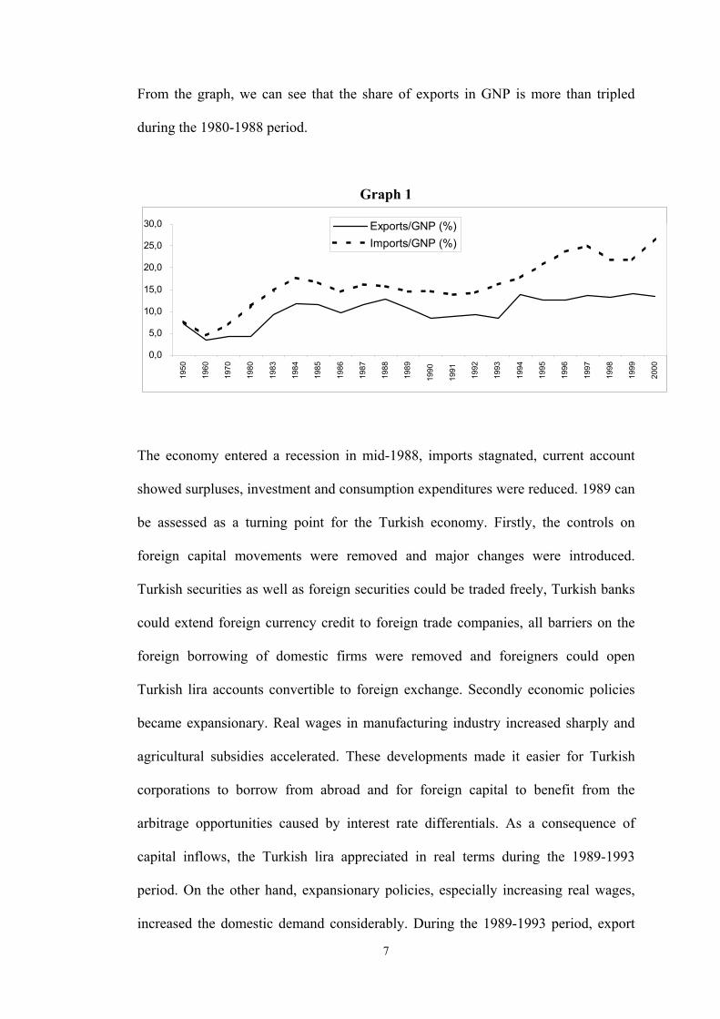
adjustment program. The share of exports and imports in GNP are shown in Graph 1.

7

From the graph, we can see that the share of exports in GNP is more than tripled

during the 1980-1988 period.

Graph 1

0,0

5,0

10,0

15,0

20,0

25,0

30,0

1950

1960

1970

1980

1983

1984

1985

1986

1987

1988

1989

1990

1991

1992

1993

1994

1995

1996

1997

1998

1999

2000

Exports/GNP (%)Imports/GNP (%)

The economy entered a recession in mid-1988, imports stagnated, current account

showed surpluses, investment and consumption expenditures were reduced. 1989 can

be assessed as a turning point for the Turkish economy. Firstly, the controls on

foreign capital movements were removed and major changes were introduced.

Turkish securities as well as foreign securities could be traded freely, Turkish banks

could extend foreign currency credit to foreign trade companies, all barriers on the

foreign borrowing of domestic firms were removed and foreigners could open

Turkish lira accounts convertible to foreign exchange. Secondly economic policies

became expansionary. Real wages in manufacturing industry increased sharply and

agricultural subsidies accelerated. These developments made it easier for Turkish

corporations to borrow from abroad and for foreign capital to benefit from the

arbitrage opportunities caused by interest rate differentials. As a consequence of

capital inflows, the Turkish lira appreciated in real terms during the 1989-1993

period. On the other hand, expansionary policies, especially increasing real wages,

increased the domestic demand considerably. During the 1989-1993 period, export

8

performance slowed significantly due to domestic demand expansion and real

appreciation of the Turkish lira; and the share of exports in GNP decreased to the

levels of the early 1980s as it can be seen from Graph 1. At the same time, export

incentives, which had a strong impact on export performance, were removed to a

large extent by the end of 1988 because of budgetary constraints. As a consequence

of these developments, trade and current account deficits increased. Then

international rating institutions decreased the credit rates of Turkey. To circumvent

panic and keep the exchange rate within certain limits, the Central Bank intervened

in the foreign exchange market at the cost of decreasing reserves. However, the

demand for foreign exchange continued resulting a substantial amount of capital

outflow. This financial crisis affected the real sector to a large extent leading to

negative growth rates in 1994. These developments caused sharp rises in inflation

and interest rates, whereas real wages declined significantly.

A stabilization program, similar to January 24 Decisions, was announced by

government on April 5, 1994. This stabilization program was intended to reduce the

domestic demand and increase exports via the real depreciation of the Turkish lira.

Therefore, exports expanded substantially in 1994. This policy continued until the

end of 1994 and expansionary measures were pursued with an expansion in domestic

activity in 1995, especially in 1996-1997 period. This growth tendency continued

until the first quarter of 1998 but started to decline afterwards because of the crisis in

Southeast Asia which affected the developing countries in 1997, the measures that

were taken for inflation targeting and the financial crisis that started in Russian

Federation in 1998. Those developments affected the financial and real sector of

Turkey negatively and increased trade deficit substantially. The economic

9

contraction that started at the second quarter of 1998 became deeper in 1999 because

of the world stagnation and the earthquakes occurred at August and November of

1999. In late 1999, in order to improve economy, “The Disinflation and Fiscal

Adjustment” program was initiated by the government. This program was intended

to increase economic activity by consumer spending and to decrease inflation rate.

But the increasing domestic demand and the rise in international oil prices has led to

sharp increase in imports and the share of imports in GNP reached its zenith point in

2000 as it can be seen from Graph 1.

To sum up, the increase in exports achieved in 1980-1989 can be attributed to the

policies summarized as devaluations of Turkish lira, export incentive schemes and

reduction in domestic demand. This episode ended by reverse trends in mentioned

policies and a sharp reduction in exports was realized between 1989 and 1993. On

the other hand, after 1992 an increasing trend can be observed in imports. The major

step in the liberalization of imports was the acceptance of Turkey into the European

Customs Union in 1996. After the financial crisis occurred in April 1994, as we can

see from the Graph 1, the share of exports in the GNP expanded notably relative to

the previous episodes and it keeps this level up to 2000.

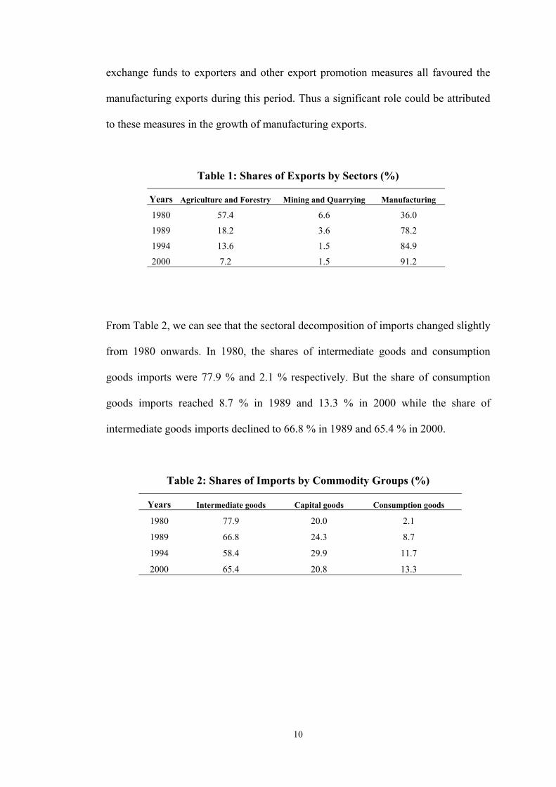
On the other hand, another important development, observable in Table 1, was that

sectoral decomposition of exports changed considerably from 1980 onwards. In

1980, the shares of agricultural and manufacturing exports were 57.4 % and 36 %

respectively. The share of agricultural exports declined to 18.2 % in 1980 and 7.2 %

in 2000 and the share of manufacturing exports reached 78.2 % in 1980 and 91.2 %

in 2000. The tax rebate system, the export credit scheme, the assignment of foreign

10

exchange funds to exporters and other export promotion measures all favoured the

manufacturing exports during this period. Thus a significant role could be attributed

to these measures in the growth of manufacturing exports.

Table 1: Shares of Exports by Sectors (%)

Years Agriculture and Forestry Mining and Quarrying Manufacturing

1980 57.4 6.6 36.0

1989 18.2 3.6 78.2

1994 13.6 1.5 84.9

2000 7.2 1.5 91.2

From Table 2, we can see that the sectoral decomposition of imports changed slightly

from 1980 onwards. In 1980, the shares of intermediate goods and consumption

goods imports were 77.9 % and 2.1 % respectively. But the share of consumption

goods imports reached 8.7 % in 1989 and 13.3 % in 2000 while the share of

intermediate goods imports declined to 66.8 % in 1989 and 65.4 % in 2000.

Table 2: Shares of Imports by Commodity Groups (%)

Years Intermediate goods Capital goods Consumption goods

1980 77.9 20.0 2.1

1989 66.8 24.3 8.7

1994 58.4 29.9 11.7

2000 65.4 20.8 13.3

11

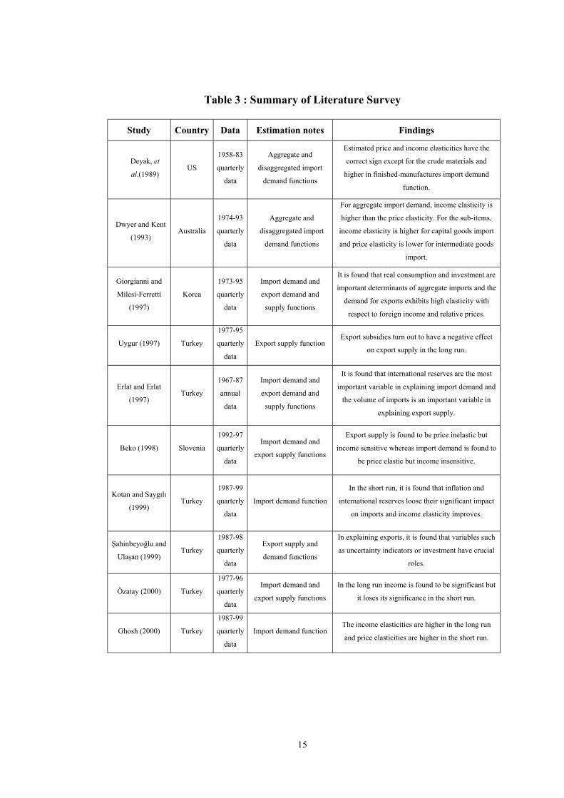
CHAPTER 3: LITERATURE SURVEY

In international trade theory, there is substantial amount of study concerning the

estimation of import demand and export supply functions and the respective income

and price elasticities. In this chapter, the empirical studies that are related to my

thesis will be analyzed briefly.

In the study by Deyak, et al. (1989), the structural stability of aggregate and

disaggregated import demand functions were estimated for US economy by using

OLS estimation techniques. In this study, import demand is disaggregated by

economic class: crude foods, crude materials, manufactured foods, semi-

manufactured foods and finished manufactures. It has been discussed that trends in

the price and income elasticities are not smoothly continuous over time and that the

values can vary considerably from one period to the next. For each import demand

function the evidence of structural instability is tested and when instability is

detected, the demand equations are reestimated along the lines suggested by the

stability tests. Estimated price and income elasticities have the correct sign except for

the crude materials and are higher in finished manufactures import demand function.

Dwyer and Kent (1993), tested the cointegration relationship between import

volumes of Australia and its explanators using the Phillips and Hansen fully

modified OLS estimator. Import volumes are considered as a function of gross

domestic product and relative price of importable goods. The import equation is also

12

estimated for the sub-items. (imports of consumption, intermediate and capital

goods) For the aggregate import demand, it is found that the income elasticity is

higher than the price elasticity. For the sub-items, the income elasticity is higher for

capital goods import and the price elasticity is lower for the intermediate goods

import.

Giorgianni and Milesi-Ferretti (1997), investigates the behaviour of Korean trade

flows and presents estimates of export demand and supply and import demand

equations. Equations are estimated by using a simultaneous structural model in

which the long and short run dynamics properties of the data are fully specified.

Estimation results indicate that real consumption and investment are important

determinants of aggregate imports and the demand for exports exhibits high elasticity

with respect to foreign income and relative prices.

Beko (1998), examined the determinants of Slovenian exports and imports by

estimating short run export supply and import demand functions for Slovene

economy using quarterly data. Total exports are considered as a function of real

exchange rate, import demand and export price index whereas total imports are

considered as a function of real exchange rate, gross domestic product and import

price index. The estimation results show that export supply is price inelastic but

income sensitive, whereas import demand is price elastic but insensitive to changes

in domestic income. It is also shown that depreciation of exchange rate have an

inflation-enhancing and growth-damaging effect in a small, open economy like

Slovenia.

13

Uygur (1997) estimated long and short run export supply functions for Turkey using

quarterly data and evaluated the export policies on the basis of the estimation results.

Long run estimation is done by Johansen’s multivariate cointegration methodology

and the short run estimation is done by taking into account an error correction term.

In the short run estimation, real exchange rate, investment, excess demand and export

subsidies significantly affect export supply with correct signs. But the export

subsidies turn out to have a negative effect on export supply in the long run.

Erlat and Erlat (1997), econometrically examined the foreign trade performance of

Turkey within the context of a three equation model consisting of export supply,

export demand and import demand. It is found that relative prices have no

explanatory power in modeling import demand and international reserves appear to

be the most important variable in explaining import demand. Also, it is found that the

volume of imports is an important variable and prices become significant only after

1980 in explaining export supply.

Kotan and Saygılı (1999), estimated an import demand function for Turkey by using

two different model specifications, Engle and Granger approach and Bernanke-Sims

structural VAR approach. It is found that in the long run, income level, nominal

depreciation rate, inflation rate and international reserves significantly affect imports.

But in the short run, inflation growth and the growth of international reserves loose

their significant impact on imports and income elasticity improves. In addition, it is

also found that, export growth and a dummy that captures the crisis in 1998 have

significant effects on import growth in the short run.

14

Şahinbeyoğlu and Ulaşan (1999), estimated export supply and export demand

functions for Turkey using quarterly data. Export supply is considered as a function

of real domestic income and real exchange rate while export demand is considered as

a function of real foreign income and real exchange rate. The estimation results

indicate that, in analyzing exports for the period after 1994, traditional export

equations are not sufficient for forecasting and policy simulations. Variables such as

uncertainty indicators or investment have crucial roles in explaining exports.

Özatay (2000), construct a quarterly macroeconometric model that describes the

functioning of the Turkish economy. In the balance of payments block of the model,

total exports are described as a function of real exchange rate and foreign income and

total imports are considered as a function of real income and real exchange rate. The

Engle and Granger two step procedure is used in the estimation of the models and the

short run dynamics is modelled as an adjustment to long run relationships. There is a

correction to the long run equilibrium every period in the short run. Estimation

results indicate that real exchange rate affects the total imports significantly both in

the long and short run, but income is significant only in the long run.

Ghosh (2000), estimated an import demand function for Turkey by using quarterly

data. Import demand is considered as a function of gross national income and real

exchange rates. Johansen estimation procedure is employed in the long run

relationship. For the long run, income elasticities vary from 2.5 to 2.8 and the price

elasticities vary from 0.05 to 0.5. An autoregressive distributed lag representation is

employed to find the short run dynamics. In the short run dynamic model, the income

elasticities vary from 0.6 to 1.7 and the price elasticities are around 0.7.

15

Table 3 : Summary of Literature Survey

Study Country Data Estimation notes Findings

Deyak, et

al.(1989)US

1958-83

quarterly

data

Aggregate and

disaggregated import

demand functions

Estimated price and income elasticities have the

correct sign except for the crude materials and

higher in finished-manufactures import demand

function.

Dwyer and Kent

(1993)Australia

1974-93

quarterly

data

Aggregate and

disaggregated import

demand functions

For aggregate import demand, income elasticity is

higher than the price elasticity. For the sub-items,

income elasticity is higher for capital goods import

and price elasticity is lower for intermediate goods

import.

Giorgianni and

Milesi-Ferretti

(1997)

Korea

1973-95

quarterly

data

Import demand and

export demand and

supply functions

It is found that real consumption and investment are

important determinants of aggregate imports and the

demand for exports exhibits high elasticity with

respect to foreign income and relative prices.

Uygur (1997) Turkey

1977-95

quarterly

data

Export supply functionExport subsidies turn out to have a negative effect

on export supply in the long run.

Erlat and Erlat

(1997)Turkey

1967-87

annual

data

Import demand and

export demand and

supply functions

It is found that international reserves are the most

important variable in explaining import demand and

the volume of imports is an important variable in

explaining export supply.

Beko (1998) Slovenia

1992-97

quarterly

data

Import demand and

export supply functions

Export supply is found to be price inelastic but

income sensitive whereas import demand is found to

be price elastic but income insensitive.

Kotan and Saygılı

(1999)Turkey

1987-99

quarterly

data

Import demand function

In the short run, it is found that inflation and

international reserves loose their significant impact

on imports and income elasticity improves.

Şahinbeyoğlu and

Ulaşan (1999)Turkey

1987-98

quarterly

data

Export supply and

demand functions

In explaining exports, it is found that variables such

as uncertainty indicators or investment have crucial

roles.

Özatay (2000) Turkey

1977-96

quarterly

data

Import demand and

export supply functions

In the long run income is found to be significant but

it loses its significance in the short run.

Ghosh (2000) Turkey

1987-99

quarterly

data

Import demand functionThe income elasticities are higher in the long run

and price elasticities are higher in the short run.

16

Having motivated from the earlier literature, this study is concerned with the

estimation of Turkish export supply and import demand equations over the period

1989-2000. Previous studies of the foreign trade of Turkey have generally

concentrated on the formulation and estimation of aggregate export and import

functions. But in Turkey, intermediate and capital goods imports are critical inputs in

the production and a model for aggregate imports may mask important differences in

the effect of income and price for sub-categories of imports. Unlike the previous

studies done for Turkey, in this study we also estimate the intermediate goods

import, capital goods import and consumption goods import demand functions. This

enable us to estimate the price and income elasticities of subitems of imports and

further discuss the policy implications of these estimates.

17

CHAPTER 4: ECONOMIC MODELLING

The theoretical foundation of export and import equations can be found in the

“imperfect substitutes” model (Goldstein and Khan (1985)). This model is based on

the simple observation that imported goods are imperfect substitutes for domestically

produced goods and that exported goods are imperfect substitutes for other countries’

domestically produced goods, or for third countries’ exports. The demand functions

can be thought of as being derived from a consumer utility maximization problem.

The consumer is assumed to maximize utility subject to a budget constraint on the

demand side. The resulting demand function for imports depends positively on

domestic income and negatively on the relative price of imported goods vis-à-vis

domestic goods. On the supply side, the producer is assumed to maximize profits

subject to a cost constraint. This yields an export supply function that depends

positively on productive capacity and export prices, and negatively on domestic

costs.

Following the Goldstein and Khan (1985) model, we consider the following

specifications for import demand and export supply:

RM = f (Y, Pm / Pd ) (1)

RX = g (Y, Px / Pd ) (2)

18

Where RM is the real quantity of imports, RX is the real quantity of exports, Y is the

real domestic income or a variable that represents productive capacity, Pd, Pm and Px

are the domestic price, import price and export price respectively. The use of relative

price ratio, instead of two separate price terms, stems from the assumption of

homogeneity and it also conveniently reduces the collinearity that may occur

between the price terms

Empirical implementation of (1) and (2) requires decisions with respect to functional

form and variable decisions. We use Gross Domestic Product (GDP) as a variable

that represents domestic income and productive capacity and Real Effective

Exchange Rate (REER) as a variable that represents the relative price ratio.

Two different real effective exchange rate indices are used in this study. The first real

effective exchange rate is calculated by using the definitionf

d

PeP

REER.1 = for

exports and the second one is calculated by using the definition

d

f

PeP

REER =2 for

imports. In these definitions, Pf indicates the foreign prices, Pd indicates the domestic

prices and e indicates the domestic currency price of foreign exchange. If we assume

barter in international trade, i.e. acquiring goods by means of exchange with other

goods, rather than with money; in the case Turkey exports to USA, REER1 implies

the quantity of USA goods that a firm in USA have to give in return of Turkish

goods and in the case USA exports to Turkey, REER2 implies the quantity of Turkish

goods that a firm in Turkey have to give in return of USA goods. So, it should be

more meaningful to use REER1 for exports and REER2 for imports.(Atuk and Öğünç,

2001)

19

There are no clear-cut criteria that can be relied on in choosing a functional form.

The choice of the form is usually based on practical considerations and intuition. For

both export supply and import demand equations, we utilize the standard log-log

specification. After the linearization, the equations of import demand and export

supply are:

RM = a0 + a1GDP + a2REER2+ ε (3)

RX = b0 + b1GDP + b2REER1+ υ (4)

The import demand equation implies that import increases as the domestic

purchasing power increases (GDP). On the contrary, when import prices increase, or

when the real effective exchange rate increases (REER2), demand of import become

less profitable and, hence, importers will supply less. From equation (3) we expect a1

to be positive and a2 to be negative.

The export supply equation implies that supply of exports increases as the prices of

exports increase, as the real effective exchange rate (REER1) decreases and also

when there is an increase in production (GDP). Therefore, we expect b1 to be

positive and b2 to be negative in equation (4).

The analysis is based on small country assumption. Since Turkey’s exports and

imports represent a small fraction of total world exports and imports, her

international price system is fully reflected by world market prices and therefore

foreign trade prices are assumed to be exogenous. In the empirical part of this study,

we will use the export supply and import demand equations specified in (3) and (4)

to estimate aggregate export supply and aggregate and disaggregated import demand.

20

CHAPTER 5: ECONOMETRIC THEORY

In this chapter, the econometric theory used in the thesis is discussed.

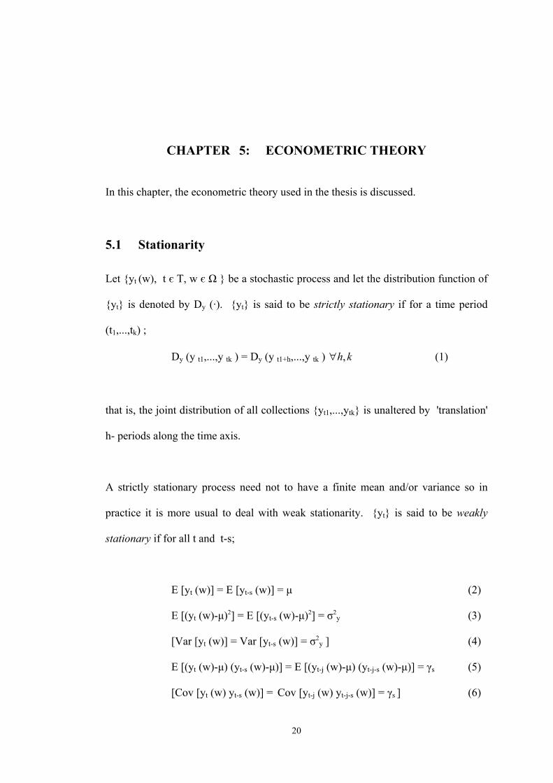
5.1 Stationarity

Let yt (w), t є Τ, w є Ω be a stochastic process and let the distribution function of

yt is denoted by Dy (·). yt is said to be strictly stationary if for a time period

(t1,...,tk) ;

Dy (y t1,...,y tk ) = Dy (y t1+h,...,y tk ) kh,∀ (1)

that is, the joint distribution of all collections yt1,...,ytk is unaltered by 'translation'

h- periods along the time axis.

A strictly stationary process need not to have a finite mean and/or variance so in

practice it is more usual to deal with weak stationarity. yt is said to be weakly

stationary if for all t and t-s;

E [yt (w)] = E [yt-s (w)] = µ (2)

E [(yt (w)-µ)2] = E [(yt-s (w)-µ)2] = σ2y (3)

[Var [yt (w)] = Var [yt-s (w)] = σ2y ] (4)

E [(yt (w)-µ) (yt-s (w)-µ)] = E [(yt-j (w)-µ) (yt-j-s (w)-µ)] = γs (5)

[Cov [yt (w) yt-s (w)] = Cov [yt-j (w) yt-j-s (w)] = γs ] (6)

21

where µ, σ2y and all γs are constants. Simply a time series is weakly stationary if its

mean and all autocovariances are unaffected by a change of time origin. In the

literature, a weakly stationary process is also referred to as a covariance stationary,

second-order stationary or wide-sense stationary process.

If one or more of the conditions above are not fullfilled, the process is nonstationary.

Nonstationarity seems a natural feature of economic life. Nonstationarity can be due

to the evolution of economy, legislative changes and technological change.

Nonstationarity of a time series is a problem in econometric analysis because when

data means and variances are non-constant, observations come from different

distributions over time, posing difficult problems for empirical modelling. Since

almost all economic data series are nonstationary, inorder to make sensible

regression analysis, these series have to be made stationary. In many cases

nonstationarity of a series can be eliminated by simple differencing. If a series must

be differenced d times to make stationary, it is said to be integrated of order d. This

is denoted as yt ~ I(d). (Granger and Newbold, 1974)

5.2 Unit Root Test

Before any sensible regression analysis can be performed, it is essential to identify

the order of integration of each variable. The general way of identifying the order of

integration is testing for a unit root. An appropriate method of testing for a unit root

has been proposed by Dickey and Fuller (1979), which is called Dickey-Fuller (DF)

test.

22

For a first order autoregressive process:

ttt pyy ε+= −1 (7)

the DF test is a test of the null hypothesis Ho : p = 1 which means yt sequence

contains a unit root. This test is based on the estimation of an equivalent regression

equation to (7), namely:

ttt yy εδ +=∆ −1 (8)

Equation (8) can be rewritten as:

ttt yy εδ ++= −1)1( (9)

which is similar to (7) with p = (1+δ). The DF test consists of testing the negativity

of δ in equation (8) where the null (Ho) and the alternative (H1) hypothesis are:

H0 : δ = 0

H1 : δ < 0

The critical values tabulated in Fuller (1976) are used to evaluate the hypothesis

because standard t-statistic does not have a limiting normal distribution under the

null hypothesis.

If the null hypothesis (H0) is rejected, it is concluded that yt is stationary (i.e. yt ~

I(0)). But if the null can not be rejected, the next step would be to test whether the

order of integration is one (i.e. ∆yt ~ I(0)). The process of differencing continues until

an order of integration is established or it is realized that series can not be made

stationary by differencing.

23

The Dickey-Fuller test is weak because it assumes that the errors (εt) are

independent and have a constant variance, and it does not take into account possible

autocorrelation in the errors. If εt is autocorrelated then the ordinary least squares

estimates of equation (8) are not efficient. The solution proposed by Dickey and

Fuller (1981) is to add lags of the dependent variable to the right-hand side of the

regression as additional explanatory variables in order to approximate the

autocorrelation. This test is called Augmented Dickey-Fuller test and it is denoted by

ADF. Among the alternative unit root tests, ADF test is found to be the most useful

in practice by Dejong, et.al. (1992) and Schwert (1987) who study the operating

characteristics of the unit root tests.

The ADF equivalent of equation (8) is the following:

∑=

−− +∆+=∆k

itititt yyy

11 εδδ (10)

The practical rule for specifying the lag length k is that; it should be relatively small

in order to save the degrees of freedom, but large enough to allow for the existence

of autocorrelation in εt.

DF and ADF tests are similar tests in that they have the same structure, they test the

same hypothesis and they use the same critical values. The only difference between

the two tests is that the ADF test includes lagged values in order to eliminate

possible autocorrelation.

24

5.3 Cointegration

If there exists a long run relationship between two (or more) nonstationary variables

and the deviations from this long run equilibrium-called the equilibrium error- are

stationary, then the variables of interest are said to be cointegrated. Intuitively,

cointegration among a set of variables implies that there exist fundamental economic

forces which make the variables move stochastically together over time.

Engle and Granger (1987) provide the following definition of cointegration. If time

series xt and yt are integrated of order d and there exists a linear combination of these

variables, say α1xt + α2yt, which is integrated of order d-b, where d ≥ b ≥ 0, then xt

and yt are said to be cointegrated of order d,b and it is denoted as xt, yt ~ CI(d,b). The

vector [α1, α2] is called the cointegrating vector. A generalization of this definition

for the case of n variables is the following: If xt denotes an n x 1 vector and each of

series in xt is I(d) and there exists an n x 1 vector α such that xt'α~I(d-b), then

xt'α~CI(d,b).

Consider the following simple regression model called the cointegration regression:

tt zx =′α (11)

where all components of xt are I(1). Stock (1987) and Engle and Granger (1987)

show that the OLS estimation of α yields an excellent approximation to the

cointegrating vector, while Cochrane-Orcutt estimation does not. The OLS estimates

of any cointegrating vector should converge to the true value extremely quickly

(Stock, 1987), however its distribution is not asymptotically normal and the

25

computed standard errors are meaningless. When xt is a vector with more than two

components, and if a cointegrating vector exists, it need not be unique; since for k

components, there may be at most r (r < k-1) linearly independent cointegrating

components. The uniqueness of the cointegrated vector between two series is shown

by Stock (1987).

Even though, there are various frameworks suggested for the analysis of

cointegration, by far the two most popular have been the Engle and Granger (1987)

and Johansen (1991) VAR approaches.

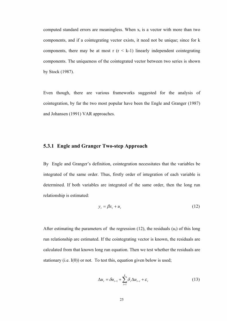
5.3.1 Engle and Granger Two-step Approach

By Engle and Granger’s definition, cointegration necessitates that the variables be

integrated of the same order. Thus, firstly order of integration of each variable is

determined. If both variables are integrated of the same order, then the long run

relationship is estimated:

ttt uxy += β (12)

After estimating the parameters of the regression (12), the residuals (ut) of this long

run relationship are estimated. If the cointegrating vector is known, the residuals are

calculated from that known long run equation. Then we test whether the residuals are

stationary (i.e. I(0)) or not. To test this, equation given below is used;

∑=

−− +∆+=∆k

itititt uuu

11 εδδ (13)

26

which is the Augmented Dickey Fuller equation. The null hypothesis is "εt is not

stationary" which implies xt and yt are not cointegrated. So, if the null hypothesis of

"εt is not stationary" is rejected we conclude that xt and yt are cointegrated. The

critical values for ADF cointegration test given in Engle and Yoo (1987) for

different sample sizes and number of observations are used to test the null hypothesis

of “no cointegration”.

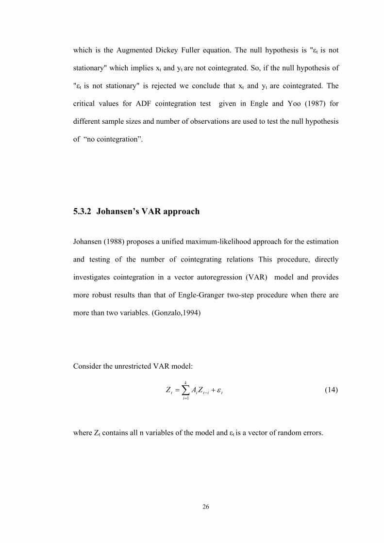
5.3.2 Johansen’s VAR approach

Johansen (1988) proposes a unified maximum-likelihood approach for the estimation

and testing of the number of cointegrating relations This procedure, directly

investigates cointegration in a vector autoregression (VAR) model and provides

more robust results than that of Engle-Granger two-step procedure when there are

more than two variables. (Gonzalo,1994)

Consider the unrestricted VAR model:

∑=

− +=k

ititit ZAZ

1

ε (14)

where Zt contains all n variables of the model and εt is a vector of random errors.

27

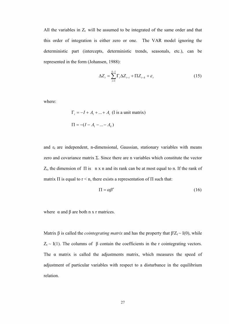
All the variables in Zt will be assumed to be integrated of the same order and that

this order of integration is either zero or one. The VAR model ignoring the

deterministic part (intercepts, deterministic trends, seasonals, etc.), can be

represented in the form (Johansen, 1988):

∑−

=−− +Π+∆Γ=∆

1

1

k

itktitit ZZZ ε (15)

where:

ii AAI +++−=Γ ...1 (I is a unit matrix)

)...( 1 kAAI −−−−=Π

and εt are independent, n-dimensional, Gaussian, stationary variables with means

zero and covariance matrix Σ. Since there are n variables which constitute the vector

Zt, the dimension of Π is n x n and its rank can be at most equal to n. If the rank of

matrix Π is equal to r < n, there exists a representation of Π such that:

βα ′=Π (16)

where α and β are both n x r matrices.

Matrix β is called the cointegrating matrix and has the property that β'Zt ~ I(0), while

Zt ~ I(1). The columns of β contain the coefficients in the r cointegrating vectors.

The α matrix is called the adjustments matrix, which measures the speed of

adjustment of particular variables with respect to a disturbance in the equilibrium

relation.

28

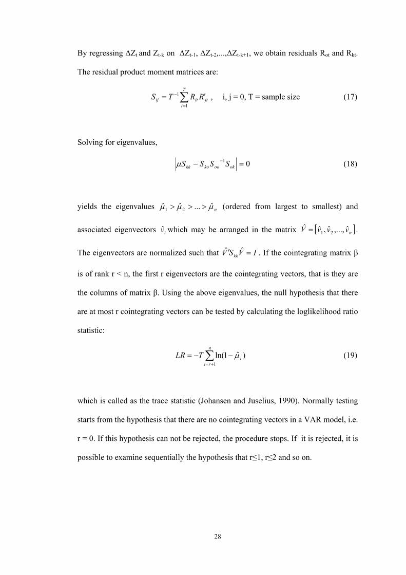
By regressing ∆Zt and Zt-k on ∆Zt-1, ∆Zt-2,...,∆Zt-k+1, we obtain residuals Rot and Rkt.

The residual product moment matrices are:

∑=

− ′=T

tjtitij RRTS

1

1 , i, j = 0, T = sample size (17)

Solving for eigenvalues,

01 =− −okookokk SSSSµ (18)

yields the eigenvalues nµµµ ˆ...ˆˆ 21 >>> (ordered from largest to smallest) and

associated eigenvectors iv which may be arranged in the matrix [ ]nvvvV ˆ,...,ˆ,ˆˆ21= .

The eigenvectors are normalized such that IVSV kk =′ ˆˆ . If the cointegrating matrix β

is of rank r < n, the first r eigenvectors are the cointegrating vectors, that is they are

the columns of matrix β. Using the above eigenvalues, the null hypothesis that there

are at most r cointegrating vectors can be tested by calculating the loglikelihood ratio

statistic:

∑+=

−−=n

riiTLR

1)ˆ1ln( µ (19)

which is called as the trace statistic (Johansen and Juselius, 1990). Normally testing

starts from the hypothesis that there are no cointegrating vectors in a VAR model, i.e.

r = 0. If this hypothesis can not be rejected, the procedure stops. If it is rejected, it is

possible to examine sequentially the hypothesis that r≤1, r≤2 and so on.

29

There is also a likelihood ratio test known as the maximum eigenvalue test in which

the null hypothesis of r cointegrated vectors is tested against the alternative of r+1

cointegrating vectors. The corresponding test statistic is:

)ˆ1ln( rTLR µ−−= (20)

The critical values of these tests are tabulated in Johansen and Juselius (1990)and

Osterwald-Lenum (1992).

In empirical applications of the Johansen method, a major problem can be met when

establishing the lag length, that is k in equation (14). If the empirical analysis is

concerned exclusively with the estimation and identification of a cointegrating

vector, the usual practice is to allow for relatively long lags. Because, long lags

might approximate the possible autocorrelation structure of the error terms.

However, if the aim is to use the estimated cointegrating vector(s) for further

analysis of the VAR model, using long lags may be inconsistent with economic

sense. In our empirical work, we will use the Schwarz criteria to choose the optimal

lag length (see Hendry (1989) for details).

Testing and analyzing cointegration by Johansen’s VAR approach is considered

superior to the Engle and Granger method due to the following reasons: first, if a

multiple cointegrating vector exists, the use of Engle-Granger method may simply

produce a complex linear combination of all the distinct cointegrating vectors that

can not be sensibly interpreted. On the other hand, Johansen’s method provides a

unified framework for the estimation and testing of cointegrating relations in the

context of VAR error correction models. Secondly, the Engle-Granger method relies

30

on a super convergence result and applies OLS in order to obtain parameter estimates

of the cointegrating vector. However, OLS parameter estimates may vary with the

arbitrary normalization implicit in the selection of the left hand side variable for the

OLS regression. In contrast, the Johansen’s method does not rely on an arbitrary

normalization. Finally, the Johansen’s procedure allows for testing certain

restrictions suggested by economic theory, such as the sign and size of the elasticity

estimates.

5.4 Error Correction Model

In an error correction model the dynamics of both short-run (changes) and long-run

(levels) adjustment processes are modelled simultaneously. This idea of

incorporating the dynamic adjustment to steady-state targets in the form of error-

correction terms, suggested by Sargan(1964) and developed by Hendry and

Anderson (1977) and Davidson et al. (1978), offers the possibility of revealing

information about both short-run and long-run relationships.

Granger (1981), Granger and Weiss (1983) and Engle and Granger (1987) have

established the connection and even the equivalence between error correction and the

concept of cointegration through the Granger representation theorem, i.e., if a set of

variables are cointegrated, then there exists a valid error correction representation,

and conversely. Cointegration thus provides a formal statistical support for the use of

ECM.

31

The n x 1 vector xt = (x1t, x2t,..., xnt)’ has an error correction representation if it can

be expressed in the form:

tptptttt xxxxx επππππ +∆++∆+∆++=∆ −−−− ...221110 (21)

where

π0 = an (n x1) vector of intercept terms with elements πio

πi = (n x n) coefficient matrices with elements πjk(i)

π = is a matrix with elements πjk such that one or more of the πjk ≠ 0

εt = an (n x 1) vector with elements εit

The disturbance terms are such that εit’s are white noise and may be correlated with

εjt.

Let all variables in xt be I(1). Now, if there is an error-correction representation of

these variables in (21), there is an linear combination of the I(1) variables that is

stationary. Solving (21) for πxt-1 yields:

∑ −∆−−∆= −− tititt xxx επππ 01 (22)

Since each expression on the right-hand side is stationary, πxt-1 must also be

stationary. Since π contains only constants, each row of π is a cointegrating vector of

xt. The first row can be written as (π11x1t-1+ π12x2t-1+ …+ π1nxnt-1). Since each series xit-1

is I(1), (π11,π12,…,π1n) must be a cointegrating vector of xt.

32

If all elements of π equal to zero, (21) is a traditional VAR in first differences. In

such circumstances, there is no error-correction representation since ∆xt does not

respond to the previous period’s deviation from long-run equilibrium.

If one or more of the πjk differs from zero, ∆xt responds to the previous period’s

deviation from long-run equilibrium. Hence, estimating xt as a VAR in the first

difference is inappropriate if xt has an error-correction representation. The omission

of the expression πxt-1 entails a misspecification error if xt has an error-correction

representation as in (21).

33

CHAPTER 6: EMPIRICAL RESULTS

In the first section of this chapter, information about the data set is provided. Then in

the following sections, the empirical results of testing stationarity and cointegration

will be presented. Finally in the last section the empirical models are estimated.

6.1 The Data Set

The data set consists of quarterly observations for the variables of interest over the

period 1989(Q1)-2000(Q4).

Turkey is an oil importing country so, due to the fact that oil imports depend strongly

on world oil prices and the changes in oil prices are considered as exogenous shocks,

the crude oil imports are excluded from total imports and intermediate goods imports

to eliminate the effects of changes in oil prices.

The nominal values for total import and its sub-items (expressed in terms of million

US dollars) have been deflated by total import price index (MPI) in order to obtain

real imports. Similarly, the nominal values for total export (expressed in terms of

million US dollars) have been deflated by total export price index (XPI) in order to

obtain real exports. The GDP data is utilized in real constant (1987) prices

(expressed in terms of billion TL).

34

Two different real effective exchange rate indices are used in this study. The first one

is calculated by using the definitionf

d

PeP

REER.1 = . In this definition, Pf indicates the

foreign prices, Pd indicates the domestic prices and e indicates the domestic currency

price of foreign exchange. While calculating this real effective exchange rate,

producer price indices of Germany and USA, the private manufacturing price index

of Turkey and the exchange rate basket which is weighted by an average of US dollar

and German mark with weights 1 and 1.5 respectively are used. An increase in

REER1 refers to an appreciation of Turkish Lira against the mentioned foreign

currencies. The second real effective exchange rate is calculated by using the

definition

d

f

PeP

REER =2 . While calculating this, for the foreign prices (Pf) consumer

price indices of Germany and USA and for the domestic prices (Pd) consumer price

index of Turkey is used. The exchange rate basket employed is the same basket that

is used in the REER1. An increase in REER2 refers to an appreciation of mentioned

foreign currencies against Turkish Lira.

The data are collected from the Central Bank of Turkey, The State Institute of

Statistics and International Financial Statistics. The data sources for all series are

given in Table 1.1 in Appendix A. The base year for all the indices is 1987 . The

data set is presented in Table 1.2 in Appendix A.

The following abbreviations are used from this part onwards:

RX: Total real export

RM: Total real non-oil import

35

RINT: Real non-oil intermediate goods import

RCAP: Real capital goods import

RCONS: Real consumption goods import

GDP: Real gross domestic product

REER1: Real effective exchange rate index calculated by using the definition

f

d

PePREER.1 =

REER2: Real effective exchange rate index calculated by using the definition

d

f

PeP

REER =2

Where L represents the logarithm, D represents the first difference

6.2 Results of Unit Root Tests

Before starting the cointegration analysis, the integration order of the series have to

be determined. The order of integration of each series is identified with unit root test.

ADF unit root tests are applied on both levels and first differences of all variables as

discussed in subsection 5.2.

The ADF test results for the levels of the variables are presented in Table 2.1 and for

the first difference of the variables are presented in Table 2.2. In both tables, the

value of “k” corresponds to the highest order lag for which the t-statistic in the

regression is significant, “C” denotes a significant intercept and “T” denotes a

significant trend and intercept.

36

Test results show that, at 5 percent significance level, the hypothesis of a unit root in

each series can not be rejected for the level of the variables but it is rejected for the

first difference of all variables. Therefore, all variables appear to be integrated of

order one (i.e. I(1)) and we have to take first difference of the variables to make them

stationary.

6.3 Results of Cointegration Tests

This section reports the results of the Engle-Granger two-step cointegration tests

(Engle and Granger, 1987) and Johansen type multivariate cointegration tests

(Johansen, 1991) among the I(1) series (LRX, LGDP, LREER1), (LRM, LGDP,

LREER2), (LRINT, LGDP, LREER2), (LRCAP, LGDP, LREER2), (LRCONS,

LGDP, LREER2)i .

6.3.1 Engle-Granger Cointegration Test Results

In the first step of Engle-Granger cointegration test, the long run equations are

estimated by OLS and results are summarized in Table 3.1 through Table 3.5 in

Appendix A. Import data and export data have a strong seasonal pattern, so the

seasonal dummies (S1, S2, S3) are included in the long run equations. The following

long run relationships are obtained from OLS estimation:

i Cointegration analysis are performed systematically among (real total exports, real income, realexchange rate), (real total imports, real income, real exchange rate), (real intermediate goods imports,

37

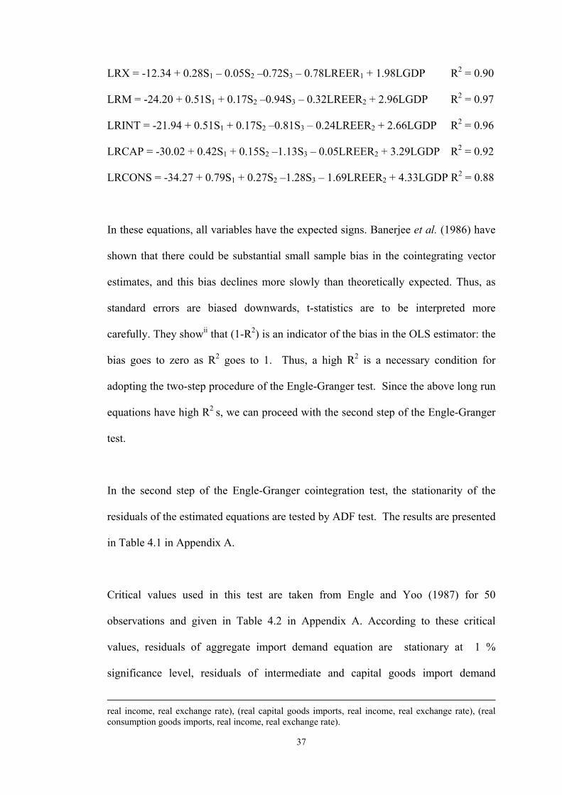
LRX = -12.34 + 0.28S1 – 0.05S2 –0.72S3 – 0.78LREER1 + 1.98LGDP R2 = 0.90

LRM = -24.20 + 0.51S1 + 0.17S2 –0.94S3 – 0.32LREER2 + 2.96LGDP R2 = 0.97

LRINT = -21.94 + 0.51S1 + 0.17S2 –0.81S3 – 0.24LREER2 + 2.66LGDP R2 = 0.96

LRCAP = -30.02 + 0.42S1 + 0.15S2 –1.13S3 – 0.05LREER2 + 3.29LGDP R2 = 0.92

LRCONS = -34.27 + 0.79S1 + 0.27S2 –1.28S3 – 1.69LREER2 + 4.33LGDP R2 = 0.88

In these equations, all variables have the expected signs. Banerjee et al. (1986) have

shown that there could be substantial small sample bias in the cointegrating vector

estimates, and this bias declines more slowly than theoretically expected. Thus, as

standard errors are biased downwards, t-statistics are to be interpreted more

carefully. They showii that (1-R2) is an indicator of the bias in the OLS estimator: the

bias goes to zero as R2 goes to 1. Thus, a high R2 is a necessary condition for

adopting the two-step procedure of the Engle-Granger test. Since the above long run

equations have high R2 s, we can proceed with the second step of the Engle-Granger

test.

In the second step of the Engle-Granger cointegration test, the stationarity of the

residuals of the estimated equations are tested by ADF test. The results are presented

in Table 4.1 in Appendix A.

Critical values used in this test are taken from Engle and Yoo (1987) for 50

observations and given in Table 4.2 in Appendix A. According to these critical

values, residuals of aggregate import demand equation are stationary at 1 %

significance level, residuals of intermediate and capital goods import demand

real income, real exchange rate), (real capital goods imports, real income, real exchange rate), (realconsumption goods imports, real income, real exchange rate).

38

equations are stationary at 5 % significance level and residuals of export supply and

consumption goods import demand equations are stationary at 10 % significance

level. Thus, all five long-run equations provide evidence in favor of cointegration

and can be used as cointegration regressions.

6.3.2 Johansen Cointegration Test Results

Johansen’s (1991) method applies the maximum likelihood procedure to determine

the presence of a cointegrating vector in a Vector Autoregression (VAR) model.

Since the cointegration results are very sensitive to the lag length of VAR, first the

optimum lag length of the cointegration analysis must be determined. We will base

our selection of the lag length on Schwarz criteria.

We start with VAR(4) due to the data limitations and the maximum lag length is

usually equal to four or five for quarterly data. The models are estimated with

including unrestricted constant term and unrestricted seasonal dummies. Removing

one lag of all the variables at a time, models are reestimated over the same sample

until the models are reduced to VAR(1). The minimum of Schwarz criteria for each

system gives the optimum lag length for the VAR models.

Schwarz test values for all models are reported in Table 5 in Appendix A. The values

in Table 5 reveal that for each model, the minimum value of the test values are

associated to VAR(1). Therefore, the optimum lag length for all models is considered

to be 1.

ii Theorem 2 in Banerjee et al. (1986, pp. 274-75)

39

After finding the optimum lag lengths as one, the Johansen cointegration test is

performed for each model. The test results are reported in Table 6.1 through 6.5 in

Appendix A. Trace and maximum eigenvalue statistics together with their 5 %

critical values are reported in the tables to decide on the number of cointegrating

vectors. According to both trace statistics and the maximum eigenvalue statistics, the

number of cointegrating vectors are one for export supply, aggregate import demand,

intermediate goods import demand, capital goods import demand and consumption

goods import demand.

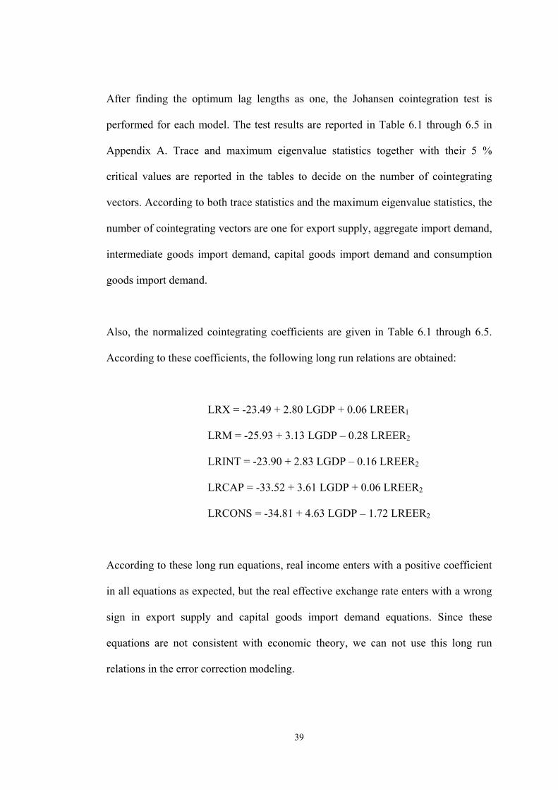
Also, the normalized cointegrating coefficients are given in Table 6.1 through 6.5.

According to these coefficients, the following long run relations are obtained:

LRX = -23.49 + 2.80 LGDP + 0.06 LREER1

LRM = -25.93 + 3.13 LGDP – 0.28 LREER2

LRINT = -23.90 + 2.83 LGDP – 0.16 LREER2

LRCAP = -33.52 + 3.61 LGDP + 0.06 LREER2

LRCONS = -34.81 + 4.63 LGDP – 1.72 LREER2

According to these long run equations, real income enters with a positive coefficient

in all equations as expected, but the real effective exchange rate enters with a wrong

sign in export supply and capital goods import demand equations. Since these

equations are not consistent with economic theory, we can not use this long run

relations in the error correction modeling.

40

In order to conduct a reliable single equation analysis, weak exogeneity of the

variables should be tested. But, since we made a small country assumption and we

found one cointegrating vector for each equation, we did not test for weak

exogeneity and proceed with single equation modelling.

6.4 Empirical Modelling

Since cointegration has been observed between variables of interest, we specify and

estimate error correction models (ECM) including the error correction terms to

investigate the dynamic behaviour of the models.

Models include the error correction terms, the residuals of the long run equations.

Since, the sign of real effective exchange rate in the long run equations of export

supply and capital goods import demand obtained in Johansen cointegration analysis

is wrong; least squares residuals are estimated from long run equations obtained in

Engle-Granger cointegration analysis. The general ECMs involve variables of

interest transformed to the I(0) space and the lag error correction terms.

For quarterly data, the maximum lag length is usually equal to four or five on the

hypothetical basis that economic agents are characterized by one-year planning

horizons. Thus, we start with fourth order autoregressive distributed lag models

(ADL) and develop these models using Hendry’s (1988) general to specific

methodology:

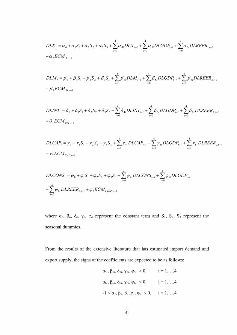
41

1,7

4

0

4

0

4

0,16543322110

−

= = =−−−

+

++++++= ∑ ∑ ∑tX

i i iitiitiitit

ECM

DLREERDLGDPDLXSSSDLX

α

ααααααα

1,7

4

0

4

0

4

0,26543322110

−

= = =−−−

+

++++++= ∑ ∑ ∑tM

i i iitiitiitit

ECM

DLREERDLGDPDLMSSSDLM

β

βββββββ

1,7

4

0

4

0

4

0,26543322110

−

= = =−−−

+

++++++= ∑ ∑ ∑tINT

i i iitiitiitit

ECM

DLREERDLGDPDLINTSSSDLINT

δ

δδδδδδδ

1,7

4

0

4

0

4

0,26543322110

−

= = =−−−

+

++++++= ∑ ∑ ∑tCAP

i i iitiitiitit

ECM

DLREERDLGDPDLCAPSSSDLCAP

γ

γγγγγγγ

1,7

4

0,26

4

0

4

0543322110

−=

−

= =−−

++

+++++=

∑

∑ ∑

tCONSi

iti

i iitiitit

ECMDLREER

DLGDPDLCONSSSSDLCONS

ϕϕ

ϕϕϕϕϕϕ

where αo, βo, δo, γo, φo represent the constant term and S1, S2, S3 represent the

seasonal dummies.

From the results of the extensive literature that has estimated import demand and

export supply, the signs of the coefficients are expected to be as follows:

α5i, β5i, δ5i, γ5i, φ5i > 0, i = 1,…,4

α6i, β6i, δ6i, γ6i, φ6i < 0, i = 1,…,4

-1 < α7, β7, δ7, γ7, φ7 < 0, i = 1,…,4

42

These expectations imply that import demand and export supply increases as real

income increases and import demand increases and export supply decreases as

Turkish Lira appreciates against the mentioned foreign currencies.

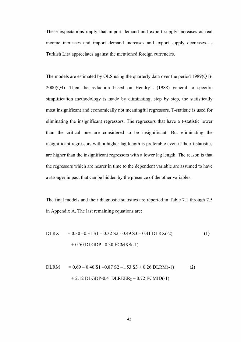
The models are estimated by OLS using the quarterly data over the period 1989(Q1)-

2000(Q4). Then the reduction based on Hendry’s (1988) general to specific

simplification methodology is made by eliminating, step by step, the statistically

most insignificant and economically not meaningful regressors. T-statistic is used for

eliminating the insignificant regressors. The regressors that have a t-statistic lower

than the critical one are considered to be insignificant. But eliminating the

insignificant regressors with a higher lag length is preferable even if their t-statistics

are higher than the insignificant regressors with a lower lag length. The reason is that

the regressors which are nearer in time to the dependent variable are assumed to have

a stronger impact that can be hidden by the presence of the other variables.

The final models and their diagnostic statistics are reported in Table 7.1 through 7.5

in Appendix A. The last remaining equations are:

DLRX = 0.30 –0.31 S1 – 0.32 S2 - 0.49 S3 – 0.41 DLRX(-2) (1)

+ 0.50 DLGDP– 0.30 ECMXS(-1)

DLRM = 0.69 – 0.40 S1 –0.87 S2 –1.53 S3 + 0.26 DLRM(-1) (2)

+ 2.12 DLGDP-0.41DLREER2 – 0.72 ECMID(-1)

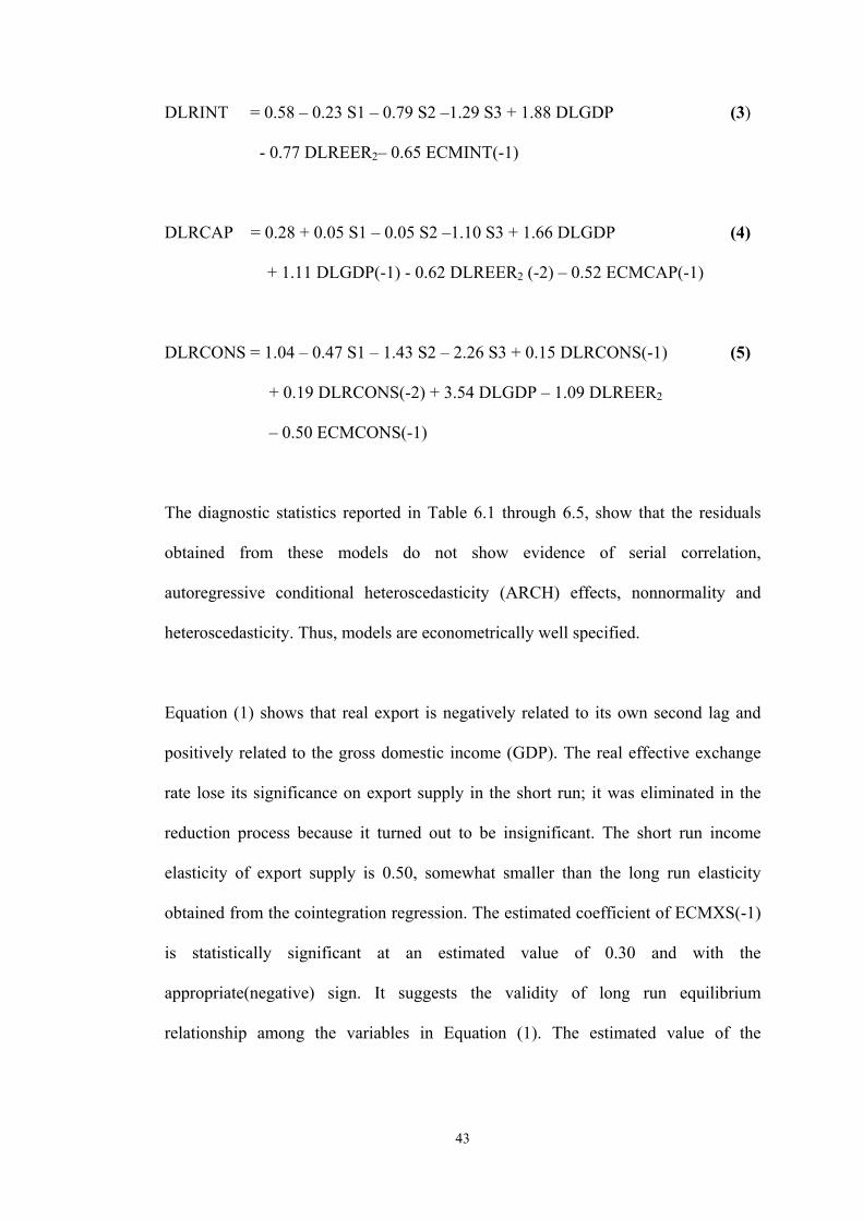
43

DLRINT = 0.58 – 0.23 S1 – 0.79 S2 –1.29 S3 + 1.88 DLGDP (3)

- 0.77 DLREER2– 0.65 ECMINT(-1)

DLRCAP = 0.28 + 0.05 S1 – 0.05 S2 –1.10 S3 + 1.66 DLGDP (4)

+ 1.11 DLGDP(-1) - 0.62 DLREER2 (-2) – 0.52 ECMCAP(-1)

DLRCONS = 1.04 – 0.47 S1 – 1.43 S2 – 2.26 S3 + 0.15 DLRCONS(-1) (5)

+ 0.19 DLRCONS(-2) + 3.54 DLGDP – 1.09 DLREER2

– 0.50 ECMCONS(-1)

The diagnostic statistics reported in Table 6.1 through 6.5, show that the residuals

obtained from these models do not show evidence of serial correlation,

autoregressive conditional heteroscedasticity (ARCH) effects, nonnormality and

heteroscedasticity. Thus, models are econometrically well specified.

Equation (1) shows that real export is negatively related to its own second lag and

positively related to the gross domestic income (GDP). The real effective exchange

rate lose its significance on export supply in the short run; it was eliminated in the

reduction process because it turned out to be insignificant. The short run income

elasticity of export supply is 0.50, somewhat smaller than the long run elasticity

obtained from the cointegration regression. The estimated coefficient of ECMXS(-1)

is statistically significant at an estimated value of 0.30 and with the

appropriate(negative) sign. It suggests the validity of long run equilibrium

relationship among the variables in Equation (1). The estimated value of the

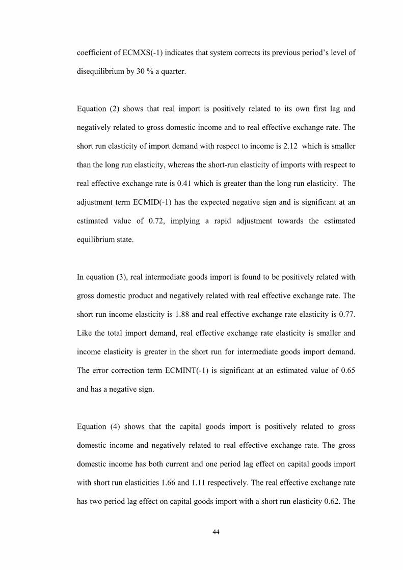
44

coefficient of ECMXS(-1) indicates that system corrects its previous period’s level of

disequilibrium by 30 % a quarter.

Equation (2) shows that real import is positively related to its own first lag and

negatively related to gross domestic income and to real effective exchange rate. The

short run elasticity of import demand with respect to income is 2.12 which is smaller

than the long run elasticity, whereas the short-run elasticity of imports with respect to

real effective exchange rate is 0.41 which is greater than the long run elasticity. The

adjustment term ECMID(-1) has the expected negative sign and is significant at an

estimated value of 0.72, implying a rapid adjustment towards the estimated

equilibrium state.

In equation (3), real intermediate goods import is found to be positively related with

gross domestic product and negatively related with real effective exchange rate. The

short run income elasticity is 1.88 and real effective exchange rate elasticity is 0.77.

Like the total import demand, real effective exchange rate elasticity is smaller and

income elasticity is greater in the short run for intermediate goods import demand.

The error correction term ECMINT(-1) is significant at an estimated value of 0.65

and has a negative sign.

Equation (4) shows that the capital goods import is positively related to gross

domestic income and negatively related to real effective exchange rate. The gross

domestic income has both current and one period lag effect on capital goods import

with short run elasticities 1.66 and 1.11 respectively. The real effective exchange rate

has two period lag effect on capital goods import with a short run elasticity 0.62. The

45

real exchange rate elasticity is greater and income elasticity is smaller in the short

run than their long-run counterparts. ECMCAP(-1) is also significant and has a value

of -0.52.

Equation (5) implies that the consumption goods import is positively related with its

own first and second lag and with gross domestic income and negatively related with

real effective exchange rate. Short run elasticity of consumption goods import with

respect to income is 3.54 and with respect to real effective exchange rate is 1.09.

Both income and real effective exchange rate elasticities are smaller in the short run

than its long run elasticities. ECMCONS(-1) is also significant and has a negative

sign. The adjustment speed towards the estimated equilibrium state is 0.50.

46

CHAPTER 7: CONCLUSION

The main purpose of this thesis is to investigate the foreign trade performance of

Turkey within the context of estimating econometric models for export supply and

import demand over the period 1989-2000. What distinguishes this study from those

previously undertaken is modeling not only total imports but also subcategories of

imports; since a model for total imports may mask important differences in the effect

of income and price for sub-categories of imports.

In empirical analysis, cointegration and error correction modeling approaches have

been used. To estimate the long run relationship between exports and imports and

related sets of variables, we applied two different types of cointegration tests: one

based on residuals from a cointegrating regression (Engle-Granger approach) and the

other is the systems-based test using the vector autoregressions (VAR) (Johansen

approach). With these tests, it has been found a unique long run equilibrium

relationship exists among the real exports, real exchange rate and real GDP and also

among the real imports (total and sub-items), real exchange rate and real GDP. In

Engle-Granger’s approach, all the variables have the expected sign but in Johansen’s

approach, real effective exchange rate enters with a wrong sign to export supply and

capital goods import demand equations. So, we estimated error correction models

based on lagged residuals from the cointegrating regressions obtained in ngle-

Granger cointegration analysis. The error correction terms in all models have found

47

to be statistically significant, suggesting the validity of the long run equilibrium

relationships.

One of the main conclusion that emerges from the empirical results is that export

supply is price (exchange rate) inelastic but income elastic in the long run whereas it

is price insensitive and income inelastic in the short run. This shows that the

depreciation of the exchange rate is not the best solution for developing strategy of

Turkish exports. More specifically, according to the export-led growth model, a

depreciation of the exchange rate can result, via the exploitation of economies of

scale, in improvement of price competitiveness and therefore in further increase of

exports only temporarily. But since imports are critical inputs into the production of

exports in Turkey, in the long run depreciation of TL would have an adverse impact

on export performance. It appears, therefore, that exchange rate policies couldn’t be

succesful in promoting export growth and the improvement of competitiveness of the

Turkish exports depends on the remodeling and updating of export supply.

Econometric estimate of aggregate import demand function suggests that import

demand is price (exchange rate) inelastic but highly elastic with respect to income

both in the short and long run. Thus, import demand is largely explained by real GDP

which relates to the general level of economic activity in the country. The low

elasticity of aggregate import demand with respect to price may partly reflect the fact

that primary commodities and raw materials constitute a large fraction of Turkish

imports.

48

The short and long run price and income elasticities for total imports and

intermediate goods imports are very close. Since approximately 65 percent of total

imports consist of intermediate goods, this is an expected result. So the intermediate

goods import demand is also price inelastic but highly elastic with respect to income

both in the short and long run which indicates that the decision to import an

intermediate good will be related primarily to economic activity.

As investments in Turkey are financed mainly with foreign capital and it takes time

to make a decision on investment, the real exchange rate affects capital goods import

demand two periods before in the short run. The capital goods import demand is also

price inelastic but income elastic both in the short and long run. This indicates, like

the intermediate goods imports, the capital goods imports are related mostly with the

economic activity.

On the other hand, consumption goods import demand is price and income elastic

and the respective elasticities are higher than those of other items both in the short

and long run. This reflects the responsiveness of consumption decisions generally to

changes in prices, given the availability of substitutes.

High values of income elasticities and low values of price elasticies means that,

except consumption goods import, import developments are highly dependent on the

economic activity and the effects of exchange rate policy on imports appear to be

fairly limited.

49

The coefficient of the error correction term in the export supply model is smaller

than that in import demand model. This indicates that the export supply model has

low speed of adjustment and hence a prolonged period of disequilibrium in the

markets before attaining long run equilibrium.

According to presented empirical results of Turkish exports and imports, we can say

that, from an economic point of view, depreciation of TL would not be the best

solution for helping exporters in a small, open economy like Turkey. As shown by

Bole (1992), this approach would work better in large economies where the domestic

market is not yet saturated and exports represent a smaller ratio to GDP. In Turkey,

depreciation of TL would lead to an increase in interest rates, thus increasing other

costs and hampering economic growth.

When we compare our results with other studies done for Turkey; Kotan and Saygılı

(1999) who estimated import demand function for Turkey, found that the exchange

rate is the most effective policy tool on import demand. However, we found that the

effects of exchange rate policy on imports appear to be fairly limited.

Şahinbeyoğlu and Ulaşan (1999) estimated export supply and export demand

functions for Turkey and found that Turkish exports are dominantly explained by

real exchange rate in the short run which is an opposite result of ours. We found that

export supply is price inelastic in the long run and price insensitive in the short run.

50

Özatay (2000) investigated import demand and export supply functions within the

context of a macroeconometric model that describes the functioning of the Turkish

economy and he found that income affects total imports significantly only in the

short run. However, we found that import demand is largely explained by income

both in the short and long run.

Ghosh (2000) estimated an import demand function for Turkey and he found that the

income elasticity is higher in the long run and price elasticity is higher in the short

run for aggregate import demand which is a consistent result with ours.

51

BIBLIOGRAPHY

Atuk, Oğuz and Fethi Öğünç. 2001. “Reel Efektif Kur Hesaplamaları: TürkiyeUygulaması.” Paper presented at 2nd Statistics Congress held in Belconti Hotel,Antalya, Turkey, May 2, 5.

Banerjee, Anindya and et al. 1993. Co-integration, Error Correction, and theEconometric Analysis of Nonstationary Data. New York: Oxford University Press.

Beko, Jani. 1998. “ Analysis of Import Demand and Export Supply in Slovenia-Empirical Regularities and Stylized Facts,” Univerza V Mariboru, EDP WorkingPapers, UDC 33.

Bhagwati, Jagdish N. 1987. International Trade: Selected Readings. London: MITPress.

Cerra, Valerie, and Anuradha Dayal-Gulati. 1999. “China’s Trade Flows: ChangingPrice Sensitivities and the Reform Process,” IMF Working Paper 99/1.

Dagenais, Marcel G. and Pierre Alain Muet. 1992. International Trade Modelling.London: Chapman & Hall.

Dejong, David N., J. S. Nankervis and Charles Whiteman. 1992. “The PowerProblems of Unit Root Tests in Time Series with Autoregressive Errors,” Journal ofEconometrics 53: 323-44

Deyak, T. A. , W. C. Sawyer and R. L. Sprinkle. 1989. “An Examination ofStructural Stability of Disaggregated US Import Demand”, Review of Economics andStatistics 71: 337-341

Dickey, David A. and Wayne A. Fuller. 1981. “Likelihood Ratio Test Statistics forAutoregressive Time Series with a Unit Root,” Econometrica 49:1057-72.

Dutta, Dilip, and Nasiruddin Ahmed. 1999. “An Aggeregate Import DemandFunction for Bangladesh: a Cointegration Approach,” Applied Economics 31: 465-472.

Dwyer, Jacqueline, and Christopher Kent. 1993. “A Re-examination of theDeterminants of Australia’s Imports,” Reserve Bank of Australia ResearchDiscussion Paper 9312.

52

Engle, Robert F. and Byung Sam Yoo. 1987. “Forecasting and Testing inCointegrated Systems,” Journal of Econometrics 35(1):143-159.

Engle, Robert F. and Clive W. J. Granger. 1987. “Cointegration and ErrorCorrection: Representation, Estimation and Testing,” Econometrica 55: 251-76.

Engle, Robert F. and Clive W. J. Granger. 1991. Long-Run Economic relationships.New York: Oxford University Press.

Erlat, Haluk, and Güzin Erlat. 1997. „The Long-Run Relationship between Terms ofTrade and Trade Balance in Turkey,” Research in Middle East Economics 2: 125-144.

Ghosh, A. R. 2000. “Turkey’s External Current Account,” International MonetaryFund Country Reports 14.

Giorgianni, Lorenzo, and Gian Maria Milesi-Ferretti. 1997. “Determinants of KoreanTrade Flows and their Geographical Destination,” IMF Working Paper 97/54.

Goldstein, Morris, and Mohsin S. Khan. 1985. “Income and Price effects in foreigntrade,” Handbook of International Economics II: 1041-105.

Gonzalo, J. 1994. “Five Alternative Methods of Estimating Long-Run EquilibriumRelationships,” Econometrica, 60: 203-33.

Granger, Clive W.J. and Andrew A.Weiss. 1983. “Time Series Analysis of ErrorCorrection Models”, in S. Karlin, T. Amemiya and L. A. Goodman (eds.), Studies inEconometrics, Time Series and Multivariate Statistics NewYork: Academic Press.

Granger, Clive W. J. And P. Newbold. 1974. “Sprious Regressions inEconometrics,” Journal of Econometrics, 2: 111-120.

Hendry, David F. and G. J. Anderson. 1977. “Testing Dynamic Specification inSmall Simultaneous Models,” Frontiers of Quantitative Economics iii(a): 361-83.

Hendry, David F. 1989. “An Interactive Economic Modelling System” Institute ofEconomics and Statistics, Oxford University, Oxford.

Johansen, Soren. 1988. “Statistical Analysis of Cointegration Vectors,” Journal ofEconomic Dynamics and Control 12: 231-54.

Johansen, Soren. 1991. “Estimation and Hypothesis Testing of Cointegration Vectorsin Gaussian Vector Autoregressive Models,” Econometrica 59:1551–1580.

Johansen, Soren. 1995. Likelihood-based Inference in Cointegrated VectorAutoregressive Models. Oxford University Press.

Johansen Soren, and Katarina Juselius. 1990. “Maximum Likelihood Estimation andInference on Cointegration- with Applications to the Demand for Money,” OxfordBulletin of Economics and Statistics 52:169-210.

53

Kotan, Zelal, and Mesut Saygılı. 1999. “Estimating an Import Function for Turkey,”Central Bank of the Republic of Turkey Discussion Paper 9909.

Mah, Jai Sheen. 1994. “Japanese Import Demand Behaviour: The CointegrationApproach,” Journal of Policy Modelling 16(3): 291-298.

Özatay Fatih. 2000. “A Quarterly Macroeconometric Model for a Highly Inflationaryand Indebted Economy,” Economic Modelling 17(1): 1-17

Pattichis, Charalambos A. 1999. “Price and Income Elasticities of DisaggregatedImport Demand: Results from UECMs and an Application,” Applied Economics31:1061-1071.

Sargan, J. D. 1964. Wages and Prices in the United Kingdom: A Study inEconometric Methodology in P. E. Hart, G. Mills and J. K. Whitaker (eds.),Econometric Analysis for National Economic Planning, Butterworth, London

Schwert, William G. 1987. “Effects of Model Specification of Tests for Unit Root inMacroeconomics Data,” Journal of Monetary Economics, 20: 73-103.

Sinha, Dipendra. 1997. “Behaviour of Import Demand in India: A CointegrationApproach,” Indian Journal of Applied Economics 6: 97-109

Şahinbeyoğlu, Gülbin, and Bülent Ulaşan. 1999. “An Empirical Examination of theStructural Stability of Export Function: The Case of Turkey,” Central Bank of theRepublic of Turkey Discussion Paper 9907.

Stock, James H. 1987. “Asymptotic Properties of Least Squares Estimators ofCointegrated Vectors,” Econometrica 55: 1035-56.

Togan, Sübidey. 1993. “The Foreign Trade Regime and Liberalization of ForeignTrade in Turkey During the 1980s,” Turkish Eximbank, Ankara.

Uygur, Ercan. 1991. “Policy, Trade and Growth in Turkey: 1970-1990,” CentralBank of the Republic of Turkey Discussion Paper 9103.

Uygur, Ercan. 1997. “Export Policies and Export Performance: The Case of Turkey,”ERF Working Paper Series 9707.

Vanek, Jaroslav. 1962. International Trade: Theory and Economic Policy. Illinois:Homewood.

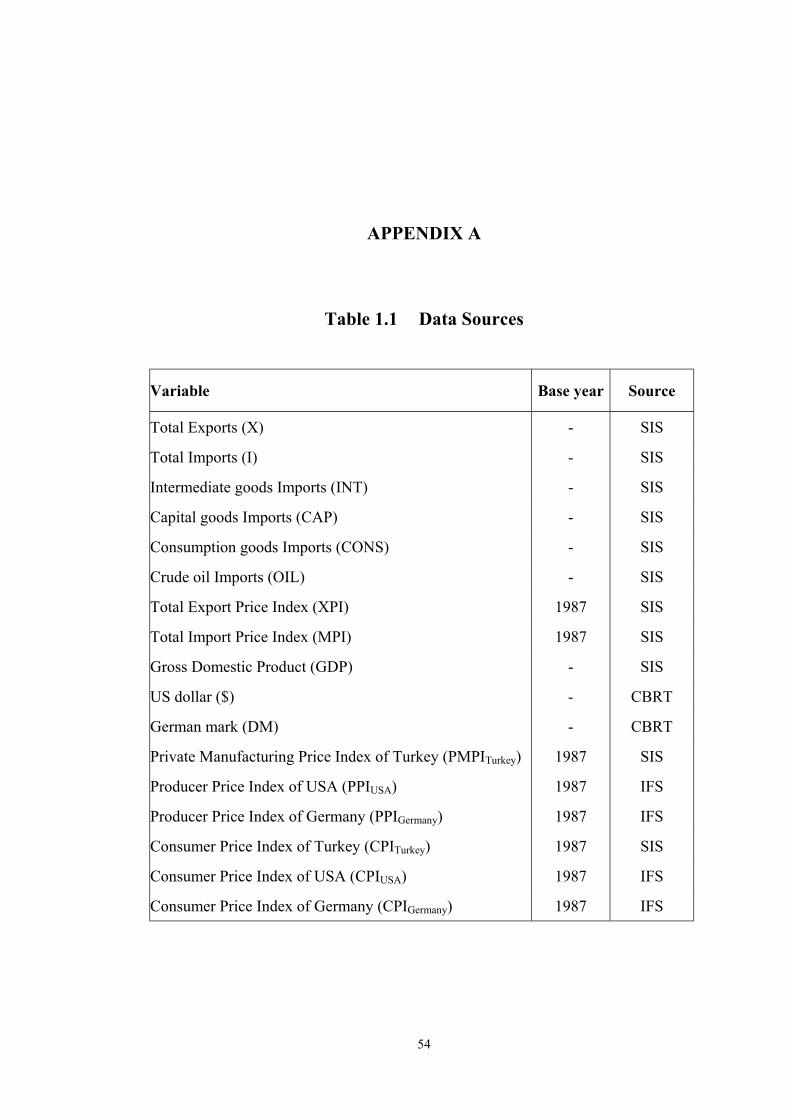
54

APPENDIX A

Table 1.1 Data Sources

Variable Base year Source

Total Exports (X) - SIS

Total Imports (I) - SIS

Intermediate goods Imports (INT) - SIS

Capital goods Imports (CAP) - SIS

Consumption goods Imports (CONS) - SIS

Crude oil Imports (OIL) - SIS

Total Export Price Index (XPI) 1987 SIS

Total Import Price Index (MPI) 1987 SIS

Gross Domestic Product (GDP) - SIS

US dollar ($) - CBRT

German mark (DM) - CBRT

Private Manufacturing Price Index of Turkey (PMPITurkey) 1987 SIS

Producer Price Index of USA (PPIUSA) 1987 IFS

Producer Price Index of Germany (PPIGermany) 1987 IFS

Consumer Price Index of Turkey (CPITurkey) 1987 SIS

Consumer Price Index of USA (CPIUSA) 1987 IFS

Consumer Price Index of Germany (CPIGermany) 1987 IFS

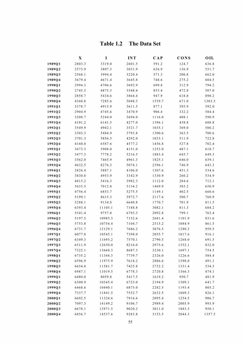
55

Table 1.2 The Data Set

X I IN T C AP C O N S O IL1989Q 1 2803.3 3319.0 2601.5 591.2 124.7 636.81989Q 2 2573.9 3807.3 3031.9 636.9 136.9 551.71989Q 3 2568.1 3994.4 3220.4 571.3 200.8 662.01989Q 4 3679.4 4671.4 3645.8 748.6 275.2 604.51990Q 1 2994.3 4706.6 3692.9 699.8 312.9 794.21990Q 2 2745.5 4875.3 3548.4 853.4 472.8 507.01990Q 3 2858.7 5434.6 3864.4 947.9 618.8 890.21990Q 4 4360.8 7285.6 5048.3 1539.7 671.0 1303.31991Q 1 3378.7 4915.9 3611.5 877.1 395.9 592.01991Q 2 2904.9 4745.6 3470.9 906.4 332.2 584.41991Q 3 3208.7 5244.0 3694.0 1116.0 408.1 590.91991Q 4 4101.2 6141.5 4277.0 1396.1 438.8 688.81992Q 1 3549.9 4942.1 3521.7 1035.1 369.0 506.21992Q 2 3303.3 5484.9 3793.8 1300.6 363.5 700.61992Q 3 3701.3 5856.5 4292.0 1033.1 511.9 722.81992Q 4 4160.0 6587.6 4577.2 1456.8 527.8 702.41993Q 1 3673.3 5908.0 4151.0 1253.0 487.1 618.71993Q 2 3477.3 7778.2 5216.5 1883.4 645.7 649.31993Q 3 3562.0 7465.9 4961.3 1825.1 646.0 639.11993Q 4 4632.5 8276.3 5074.1 2396.1 746.9 643.31994Q 1 3826.4 5887.1 4106.0 1307.6 451.3 534.61994Q 2 3830.8 4953.9 3342.9 1330.9 260.2 534.91994Q 3 4815.2 5416.3 3982.3 1112.0 284.6 712.11994Q 4 5633.5 7012.8 5134.2 1469.9 385.2 650.91995Q 1 4756.4 6853.7 5275.5 1149.1 402.5 660.61995Q 2 5199.1 8615.3 5972.7 2117.6 500.7 760.91995Q 3 5288.1 9134.8 6640.8 1770.7 701.9 811.51995Q 4 6393.4 11105.1 7188.8 3082.1 811.3 684.21996Q 1 5541.4 9757.8 6793.3 2092.8 799.1 763.41996Q 2 5197.5 10985.3 7152.6 2681.4 1101.9 831.61996Q 3 5753.8 10754.4 7104.7 2515.2 1084.9 861.51996Q 4 6731.7 12129.1 7686.2 3076.5 1280.3 959.51997Q 1 6077.8 10545.1 7398.0 2055.7 1017.6 916.11997Q 2 6349.3 11695.2 7570.1 2790.5 1268.0 691.51997Q 3 6511.9 12650.0 8216.0 2975.6 1352.1 832.01997Q 4 7322.1 13668.3 8687.3 3230.1 1697.1 754.51998Q 1 6735.2 11344.3 7739.7 2326.0 1226.6 584.41998Q 2 6596.9 11975.9 7618.2 2886.6 1398.0 491.11998Q 3 6654.8 11581.7 7425.8 2732.2 1331.4 534.31998Q 4 6987.1 11019.5 6778.3 2720.8 1366.3 474.11999Q 1 6480.0 8059.8 5417.5 1619.2 950.7 481.91999Q 2 6300.9 10345.4 6723.0 2194.9 1309.1 641.71999Q 3 6468.6 10440.1 6875.0 2282.5 1193.4 805.21999Q 4 7337.7 11841.5 7552.7 2632.5 1609.3 826.12000Q 1 6692.5 11324.6 7916.6 2095.4 1254.5 906.72000Q 2 7097.3 14149.2 9106.7 2989.4 2005.9 993.92000Q 3 6678.1 13971.5 9020.2 3011.0 1883.3 950.12000Q 4 6856.7 14537.6 9283.8 3153.5 2044.3 1357.5

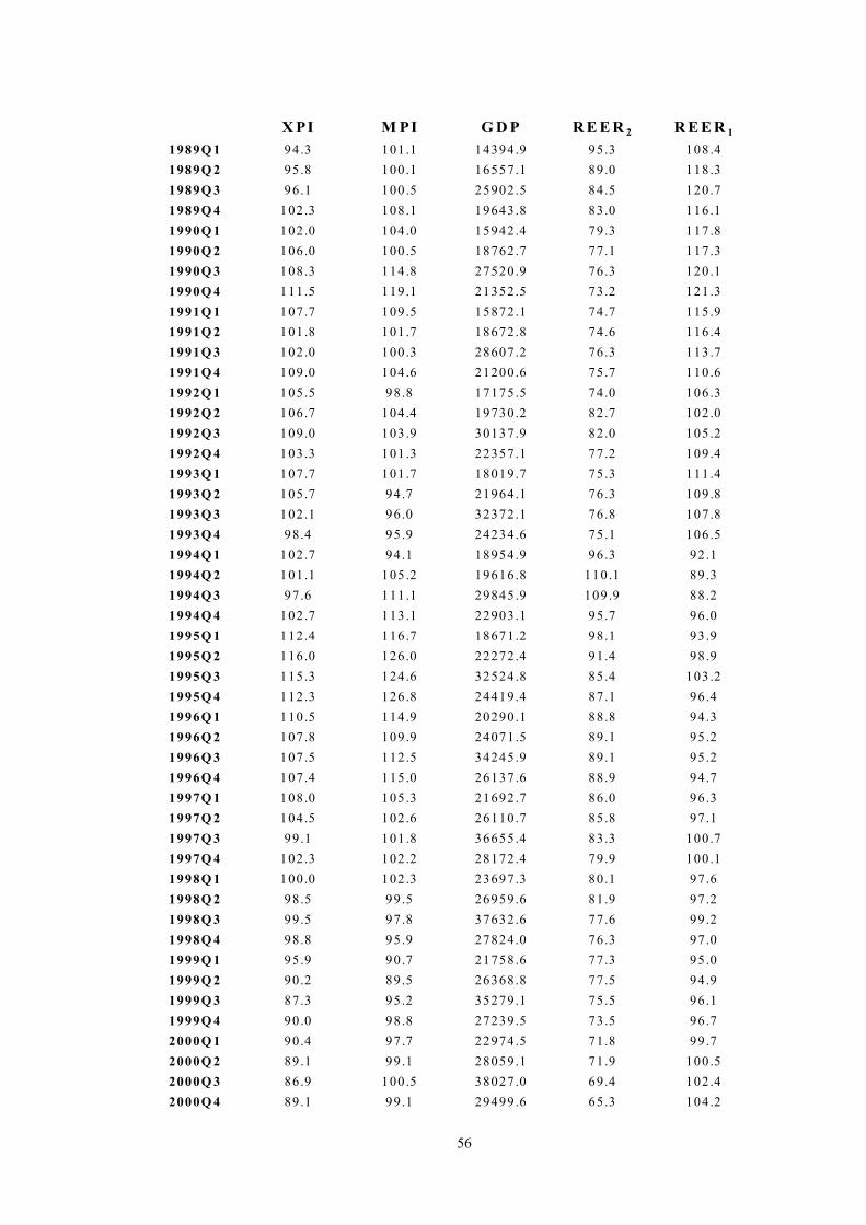
56

X PI M PI G D P R E E R 2 R E E R 1

1989Q 1 94.3 101 .1 14394.9 95.3 108 .41989Q 2 95.8 100 .1 16557.1 89.0 118 .31989Q 3 96.1 100 .5 25902.5 84.5 120 .71989Q 4 102.3 108 .1 19643.8 83.0 116 .11990Q 1 102.0 104 .0 15942.4 79.3 117 .81990Q 2 106.0 100 .5 18762.7 77.1 117 .31990Q 3 108.3 114 .8 27520.9 76.3 120 .11990Q 4 111.5 119 .1 21352.5 73.2 121 .31991Q 1 107.7 109 .5 15872.1 74.7 115 .91991Q 2 101.8 101 .7 18672.8 74.6 116 .41991Q 3 102.0 100 .3 28607.2 76.3 113 .71991Q 4 109.0 104 .6 21200.6 75.7 110 .61992Q 1 105.5 98.8 17175.5 74.0 106 .31992Q 2 106.7 104 .4 19730.2 82.7 102 .01992Q 3 109.0 103 .9 30137.9 82.0 105 .21992Q 4 103.3 101 .3 22357.1 77.2 109 .41993Q 1 107.7 101 .7 18019.7 75.3 111 .41993Q 2 105.7 94.7 21964.1 76.3 109 .81993Q 3 102.1 96.0 32372.1 76.8 107 .81993Q 4 98.4 95.9 24234.6 75.1 106 .51994Q 1 102.7 94.1 18954.9 96.3 92.11994Q 2 101.1 105 .2 19616.8 110 .1 89.31994Q 3 97.6 111 .1 29845.9 109 .9 88.21994Q 4 102.7 113 .1 22903.1 95.7 96.01995Q 1 112.4 116 .7 18671.2 98.1 93.91995Q 2 116.0 126 .0 22272.4 91.4 98.91995Q 3 115.3 124 .6 32524.8 85.4 103 .21995Q 4 112.3 126 .8 24419.4 87.1 96.41996Q 1 110.5 114 .9 20290.1 88.8 94.31996Q 2 107.8 109 .9 24071.5 89.1 95.21996Q 3 107.5 112 .5 34245.9 89.1 95.21996Q 4 107.4 115 .0 26137.6 88.9 94.71997Q 1 108.0 105 .3 21692.7 86.0 96.31997Q 2 104.5 102 .6 26110.7 85.8 97.11997Q 3 99.1 101 .8 36655.4 83.3 100 .71997Q 4 102.3 102 .2 28172.4 79.9 100 .11998Q 1 100.0 102 .3 23697.3 80.1 97.61998Q 2 98.5 99.5 26959.6 81.9 97.21998Q 3 99.5 97.8 37632.6 77.6 99.21998Q 4 98.8 95.9 27824.0 76.3 97.01999Q 1 95.9 90.7 21758.6 77.3 95.01999Q 2 90.2 89.5 26368.8 77.5 94.91999Q 3 87.3 95.2 35279.1 75.5 96.11999Q 4 90.0 98.8 27239.5 73.5 96.72000Q 1 90.4 97.7 22974.5 71.8 99.72000Q 2 89.1 99.1 28059.1 71.9 100 .52000Q 3 86.9 100 .5 38027.0 69.4 102 .42000Q 4 89.1 99.1 29499.6 65.3 104 .2

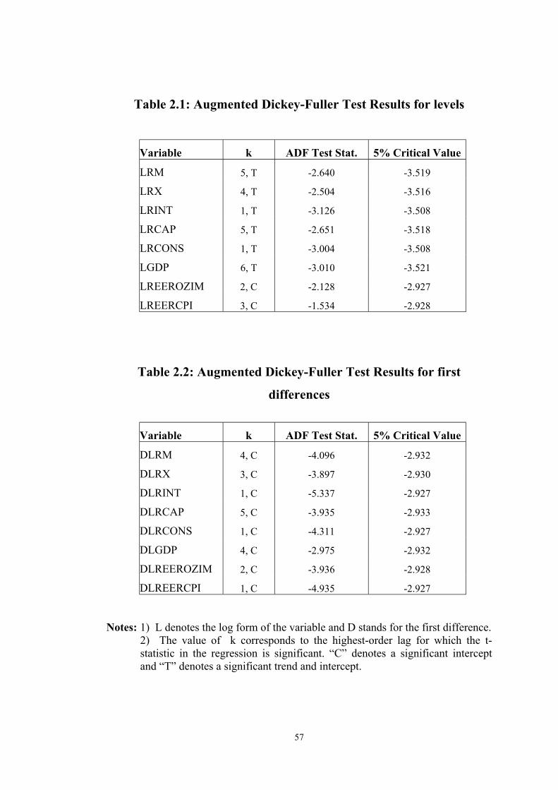
57

Table 2.1: Augmented Dickey-Fuller Test Results for levels

Variable k ADF Test Stat. 5% Critical Value

LRM 5, T -2.640 -3.519

LRX 4, T -2.504 -3.516

LRINT 1, T -3.126 -3.508

LRCAP 5, T -2.651 -3.518

LRCONS 1, T -3.004 -3.508

LGDP 6, T -3.010 -3.521

LREEROZIM 2, C -2.128 -2.927

LREERCPI 3, C -1.534 -2.928

Table 2.2: Augmented Dickey-Fuller Test Results for first

differences

Variable k ADF Test Stat. 5% Critical Value

DLRM 4, C -4.096 -2.932

DLRX 3, C -3.897 -2.930

DLRINT 1, C -5.337 -2.927

DLRCAP 5, C -3.935 -2.933

DLRCONS 1, C -4.311 -2.927

DLGDP 4, C -2.975 -2.932

DLREEROZIM 2, C -3.936 -2.928

DLREERCPI 1, C -4.935 -2.927

Notes: 1) L denotes the log form of the variable and D stands for the first difference.2) The value of k corresponds to the highest-order lag for which the t-statistic in the regression is significant. “C” denotes a significant interceptand “T” denotes a significant trend and intercept.

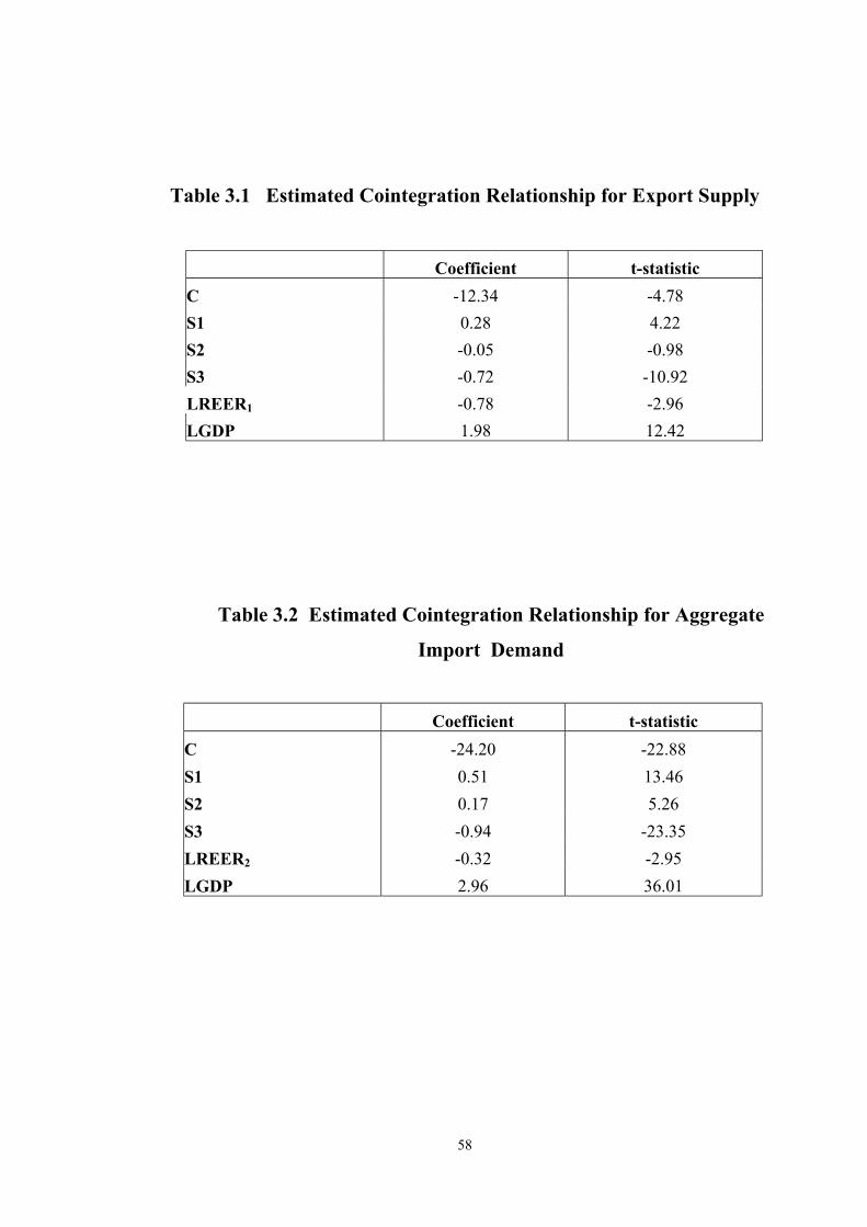
58

Table 3.1 Estimated Cointegration Relationship for Export Supply

Coefficient t-statisticC -12.34 -4.78S1 0.28 4.22S2 -0.05 -0.98S3 -0.72 -10.92LREER1 -0.78 -2.96LGDP 1.98 12.42

Table 3.2 Estimated Cointegration Relationship for Aggregate

Import Demand

Coefficient t-statisticC -24.20 -22.88S1 0.51 13.46S2 0.17 5.26S3 -0.94 -23.35LREER2 -0.32 -2.95LGDP 2.96 36.01

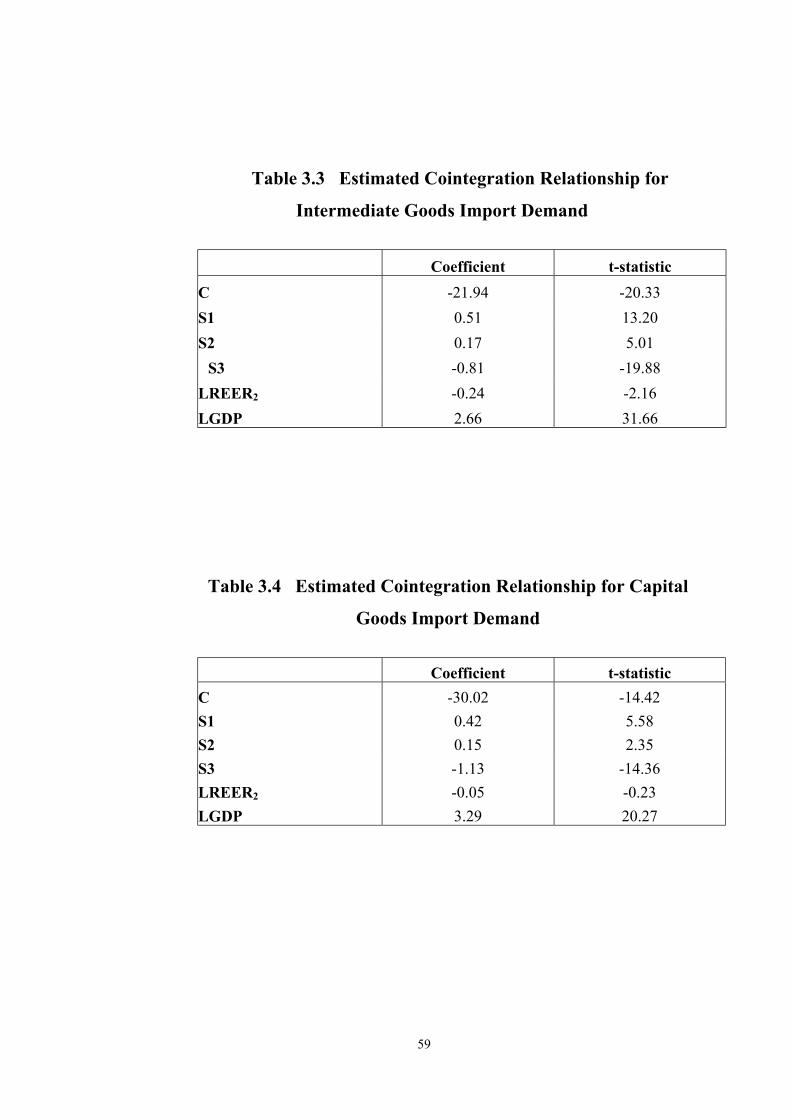
59

Table 3.3 Estimated Cointegration Relationship for

Intermediate Goods Import Demand

Coefficient t-statisticC -21.94 -20.33S1 0.51 13.20S2 0.17 5.01

S3 -0.81 -19.88LREER2 -0.24 -2.16LGDP 2.66 31.66

Table 3.4 Estimated Cointegration Relationship for Capital

Goods Import Demand

Coefficient t-statisticC -30.02 -14.42S1 0.42 5.58S2 0.15 2.35S3 -1.13 -14.36LREER2 -0.05 -0.23LGDP 3.29 20.27

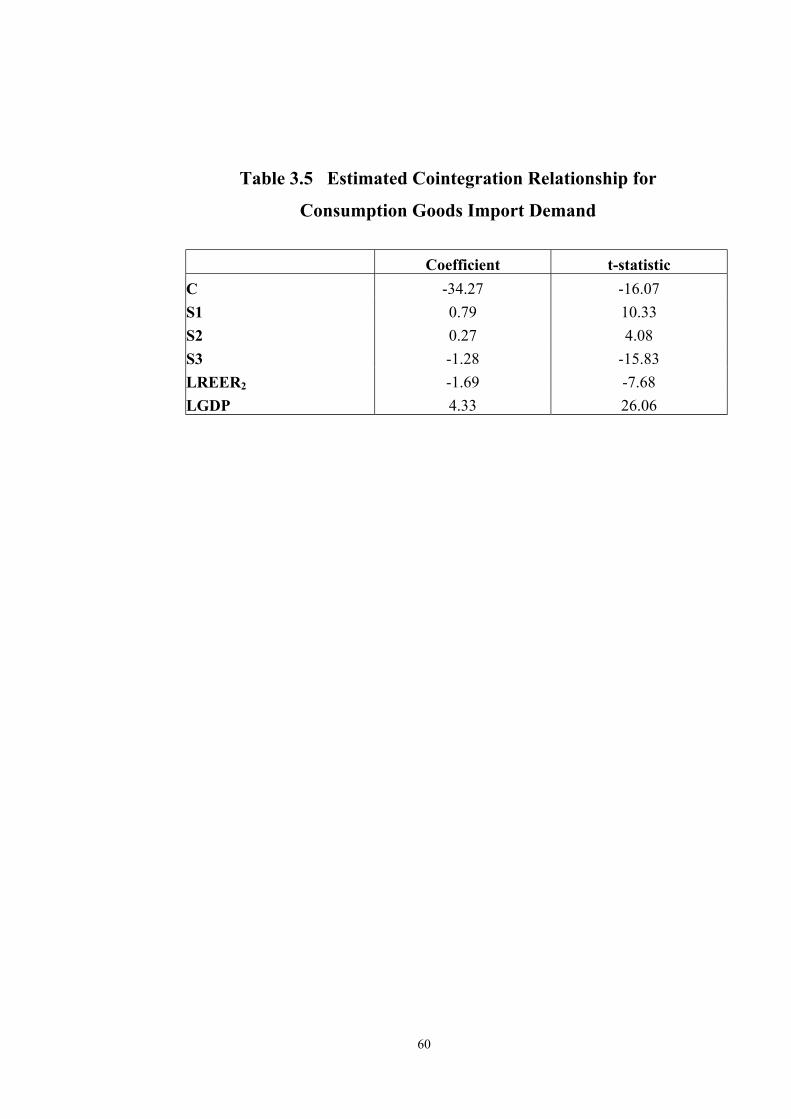
60

Table 3.5 Estimated Cointegration Relationship for

Consumption Goods Import Demand

Coefficient t-statisticC -34.27 -16.07S1 0.79 10.33S2 0.27 4.08S3 -1.28 -15.83LREER2 -1.69 -7.68LGDP 4.33 26.06

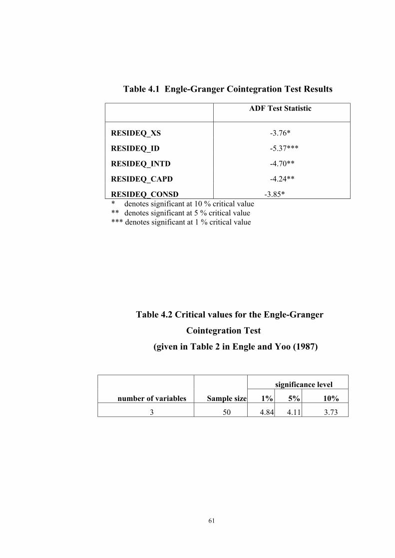
61

Table 4.1 Engle-Granger Cointegration Test Results

ADF Test Statistic

RESIDEQ_XS -3.76*

RESIDEQ_ID -5.37***

RESIDEQ_INTD -4.70**

RESIDEQ_CAPD -4.24**

RESIDEQ_CONSD -3.85** denotes significant at 10 % critical value** denotes significant at 5 % critical value*** denotes significant at 1 % critical value

Table 4.2 Critical values for the Engle-Granger

Cointegration Test

(given in Table 2 in Engle and Yoo (1987)

significance level

number of variables Sample size 1% 5% 10%

3 50 4.84 4.11 3.73

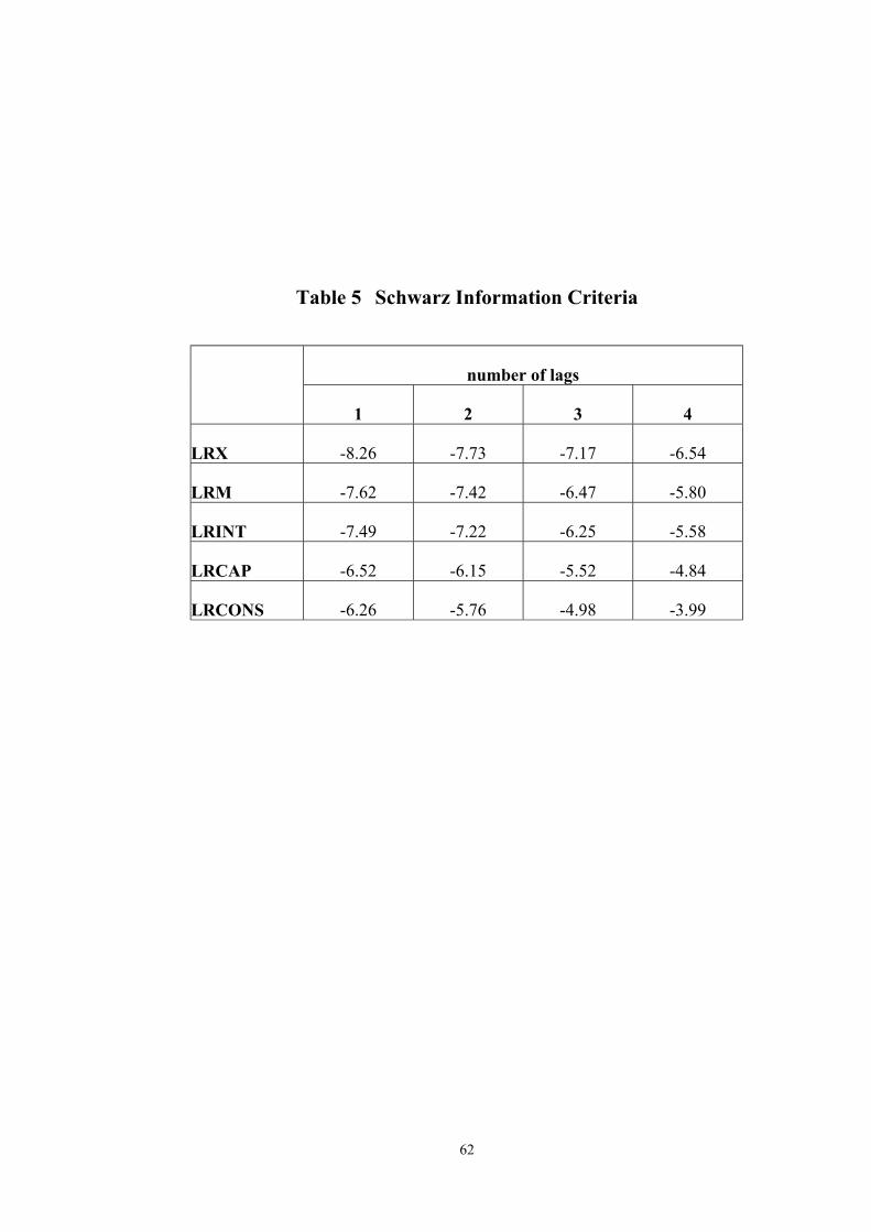
62

Table 5 Schwarz Information Criteria

number of lags

1 2 3 4

LRX -8.26 -7.73 -7.17 -6.54

LRM -7.62 -7.42 -6.47 -5.80

LRINT -7.49 -7.22 -6.25 -5.58

LRCAP -6.52 -6.15 -5.52 -4.84

LRCONS -6.26 -5.76 -4.98 -3.99

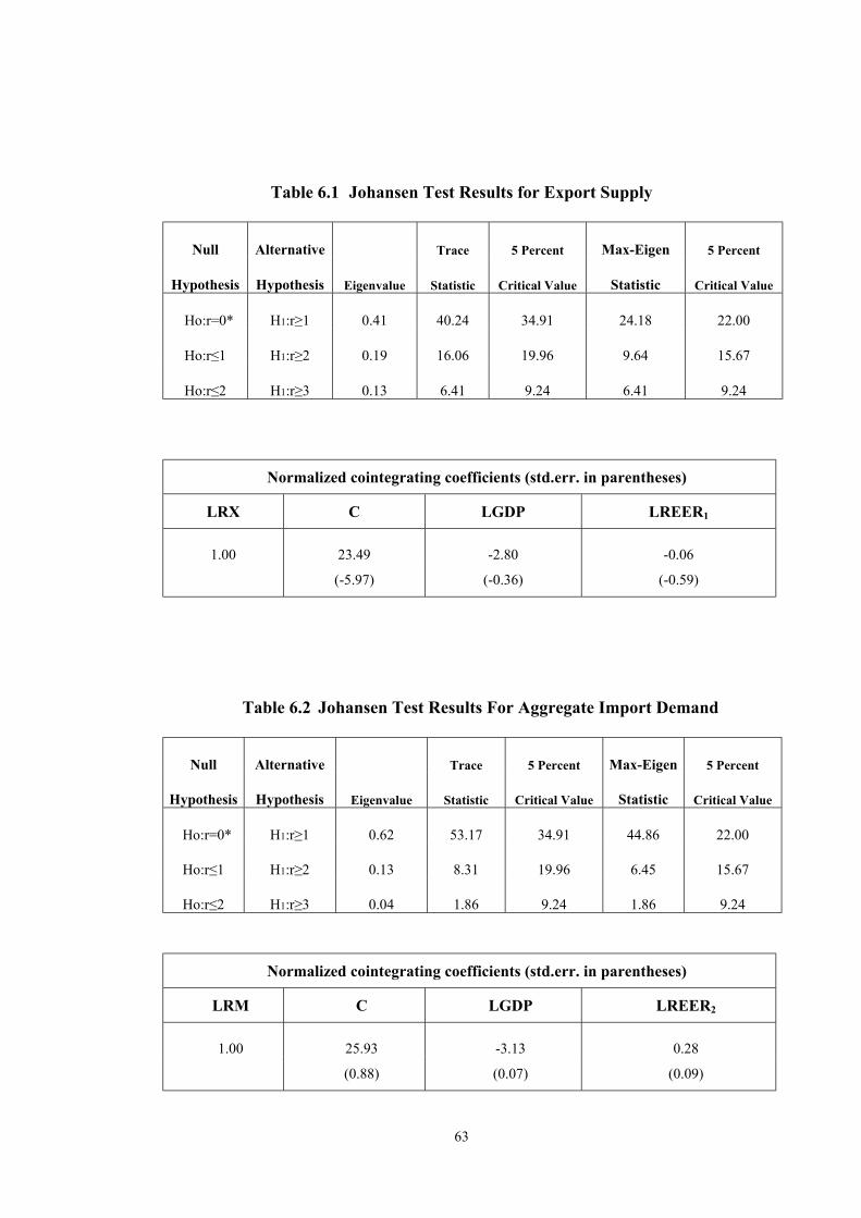
63

Table 6.1 Johansen Test Results for Export Supply

Null Alternative Trace 5 Percent Max-Eigen 5 Percent

Hypothesis Hypothesis Eigenvalue Statistic Critical Value Statistic Critical Value

Ho:r=0* H1:r≥1 0.41 40.24 34.91 24.18 22.00

Ho:r≤1 H1:r≥2 0.19 16.06 19.96 9.64 15.67

Ho:r≤2 H1:r≥3 0.13 6.41 9.24 6.41 9.24

Normalized cointegrating coefficients (std.err. in parentheses)

LRX C LGDP LREER1

1.00 23.49 -2.80 -0.06

(-5.97) (-0.36) (-0.59)

Table 6.2 Johansen Test Results For Aggregate Import Demand

Null Alternative Trace 5 Percent Max-Eigen 5 Percent

Hypothesis Hypothesis Eigenvalue Statistic Critical Value Statistic Critical Value

Ho:r=0* H1:r≥1 0.62 53.17 34.91 44.86 22.00

Ho:r≤1 H1:r≥2 0.13 8.31 19.96 6.45 15.67

Ho:r≤2 H1:r≥3 0.04 1.86 9.24 1.86 9.24

Normalized cointegrating coefficients (std.err. in parentheses)

LRM C LGDP LREER2

1.00 25.93 -3.13 0.28

(0.88) (0.07) (0.09)

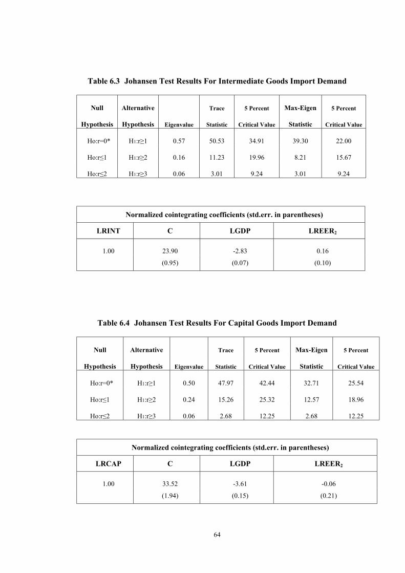
64

Table 6.3 Johansen Test Results For Intermediate Goods Import Demand

Null Alternative Trace 5 Percent Max-Eigen 5 Percent

Hypothesis Hypothesis Eigenvalue Statistic Critical Value Statistic Critical Value

Ho:r=0* H1:r≥1 0.57 50.53 34.91 39.30 22.00

Ho:r≤1 H1:r≥2 0.16 11.23 19.96 8.21 15.67

Ho:r≤2 H1:r≥3 0.06 3.01 9.24 3.01 9.24

Normalized cointegrating coefficients (std.err. in parentheses)

LRINT C LGDP LREER2

1.00 23.90 -2.83 0.16

(0.95) (0.07) (0.10)

Table 6.4 Johansen Test Results For Capital Goods Import Demand

Null Alternative Trace 5 Percent Max-Eigen 5 Percent

Hypothesis Hypothesis Eigenvalue Statistic Critical Value Statistic Critical Value

Ho:r=0* H1:r≥1 0.50 47.97 42.44 32.71 25.54

Ho:r≤1 H1:r≥2 0.24 15.26 25.32 12.57 18.96

Ho:r≤2 H1:r≥3 0.06 2.68 12.25 2.68 12.25

Normalized cointegrating coefficients (std.err. in parentheses)

LRCAP C LGDP LREER2

1.00 33.52 -3.61 -0.06

(1.94) (0.15) (0.21)

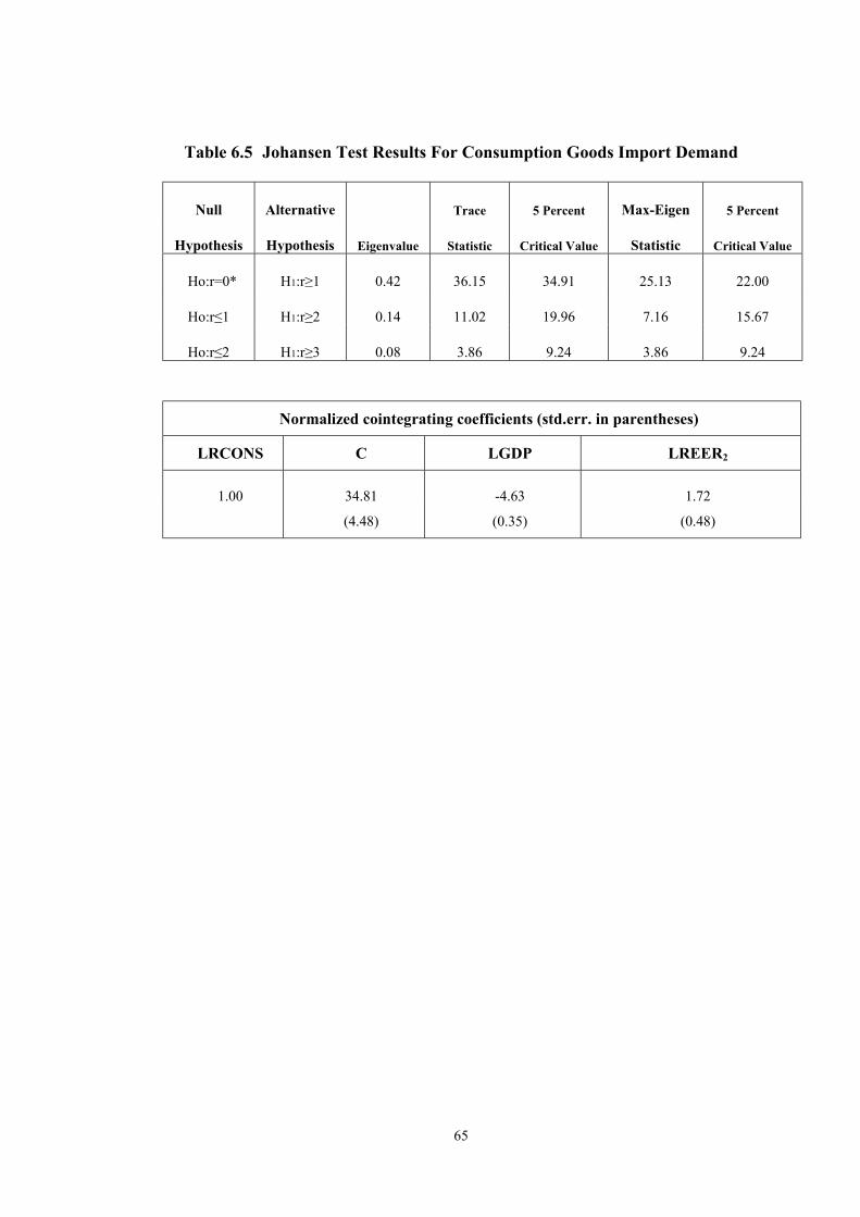
65

Table 6.5 Johansen Test Results For Consumption Goods Import Demand

Null Alternative Trace 5 Percent Max-Eigen 5 Percent

Hypothesis Hypothesis Eigenvalue Statistic Critical Value Statistic Critical Value

Ho:r=0* H1:r≥1 0.42 36.15 34.91 25.13 22.00

Ho:r≤1 H1:r≥2 0.14 11.02 19.96 7.16 15.67

Ho:r≤2 H1:r≥3 0.08 3.86 9.24 3.86 9.24

Normalized cointegrating coefficients (std.err. in parentheses)

LRCONS C LGDP LREER2

1.00 34.81 -4.63 1.72

(4.48) (0.35) (0.48)

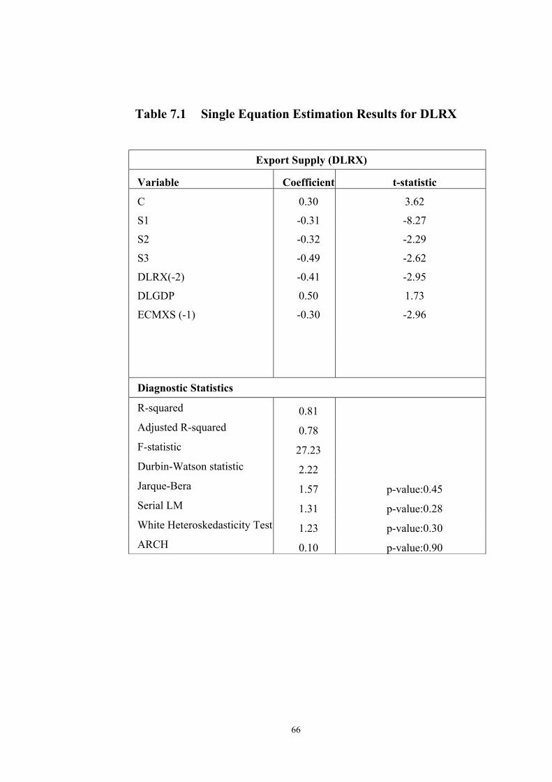
66

Table 7.1 Single Equation Estimation Results for DLRX

Export Supply (DLRX)

Variable Coefficient t-statistic

C 0.30 3.62

S1 -0.31 -8.27

S2 -0.32 -2.29

S3 -0.49 -2.62

DLRX(-2) -0.41 -2.95

DLGDP 0.50 1.73

ECMXS (-1) -0.30 -2.96

Diagnostic Statistics

R-squared 0.81 Adjusted R-squared 0.78 F-statistic 27.23 Durbin-Watson statistic 2.22 Jarque-Bera 1.57 p-value:0.45Serial LM 1.31 p-value:0.28White Heteroskedasticity Test 1.23 p-value:0.30ARCH 0.10 p-value:0.90

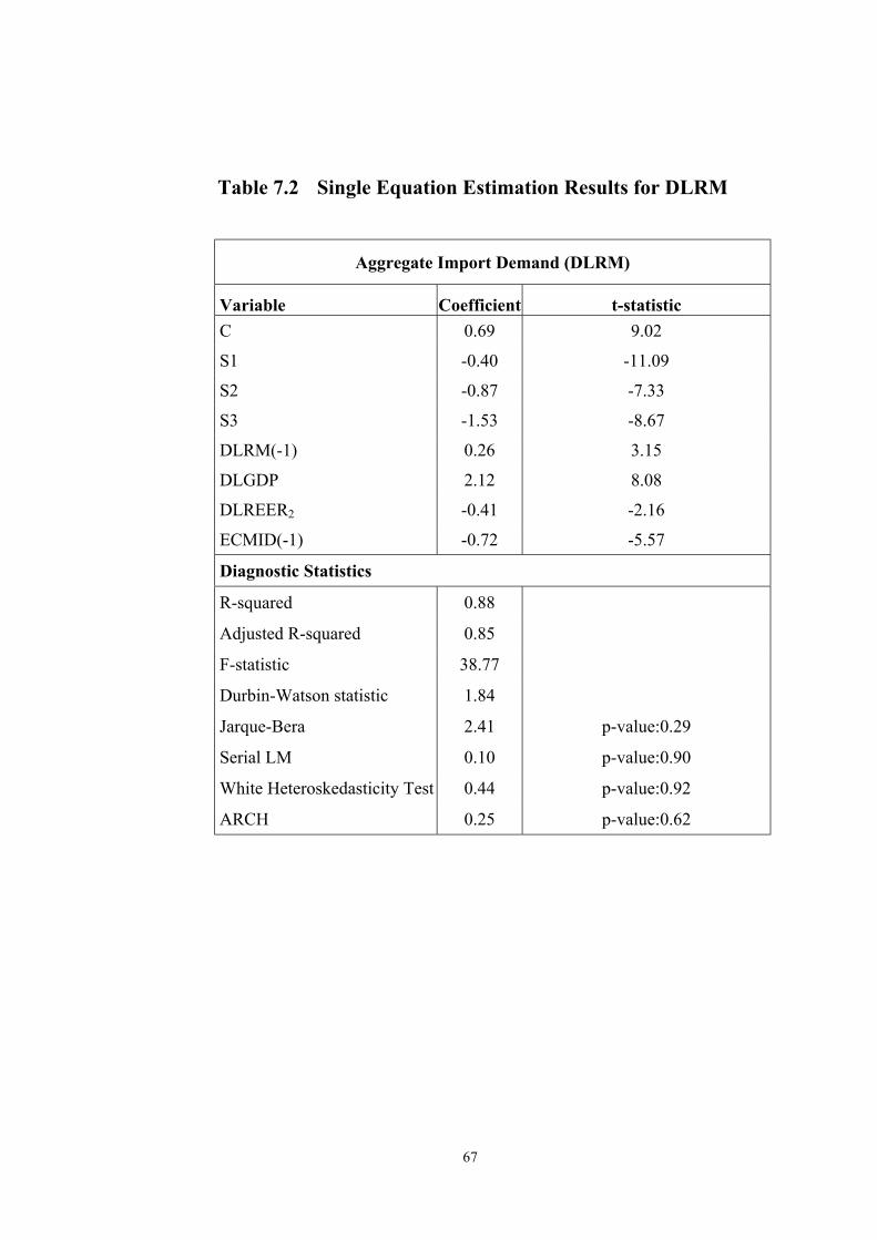
67

Table 7.2 Single Equation Estimation Results for DLRM

Aggregate Import Demand (DLRM)

Variable Coefficient t-statisticC 0.69 9.02

S1 -0.40 -11.09

S2 -0.87 -7.33

S3 -1.53 -8.67

DLRM(-1) 0.26 3.15

DLGDP 2.12 8.08

DLREER2 -0.41 -2.16

ECMID(-1) -0.72 -5.57

Diagnostic Statistics

R-squared 0.88

Adjusted R-squared 0.85

F-statistic 38.77

Durbin-Watson statistic 1.84

Jarque-Bera 2.41 p-value:0.29

Serial LM 0.10 p-value:0.90

White Heteroskedasticity Test 0.44 p-value:0.92

ARCH 0.25 p-value:0.62

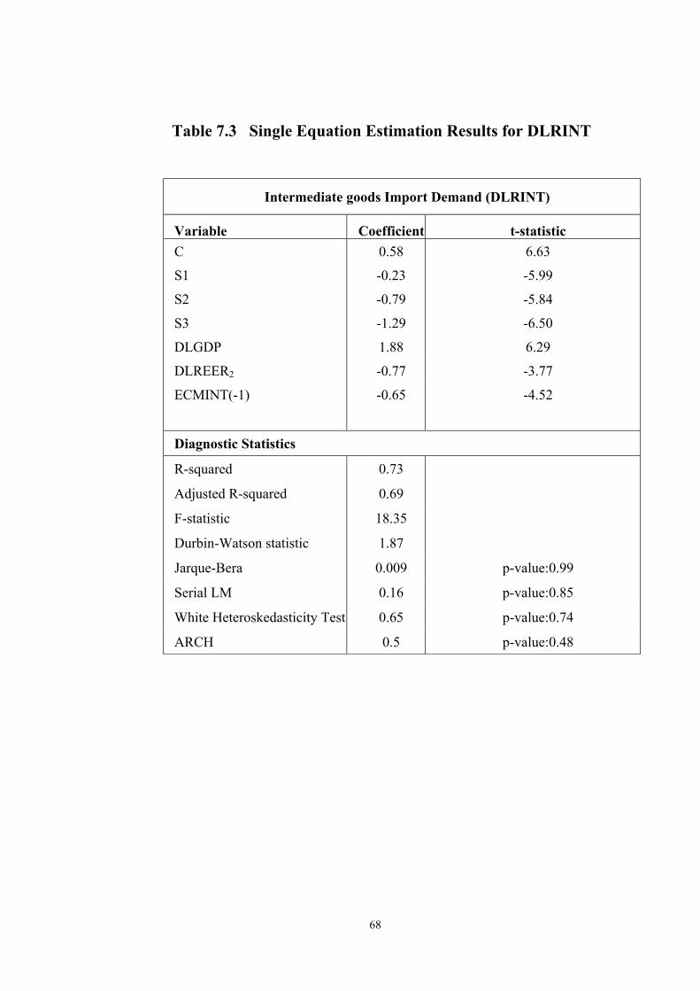
68

Table 7.3 Single Equation Estimation Results for DLRINT

Intermediate goods Import Demand (DLRINT)

Variable Coefficient t-statisticC 0.58 6.63

S1 -0.23 -5.99

S2 -0.79 -5.84

S3 -1.29 -6.50

DLGDP 1.88 6.29

DLREER2 -0.77 -3.77

ECMINT(-1) -0.65 -4.52

Diagnostic Statistics

R-squared 0.73

Adjusted R-squared 0.69

F-statistic 18.35

Durbin-Watson statistic 1.87

Jarque-Bera 0.009 p-value:0.99

Serial LM 0.16 p-value:0.85

White Heteroskedasticity Test 0.65 p-value:0.74

ARCH 0.5 p-value:0.48

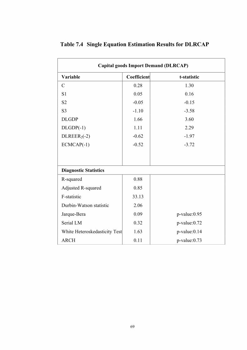
69

Table 7.4 Single Equation Estimation Results for DLRCAP

Capital goods Import Demand (DLRCAP)

Variable Coefficient t-statistic

C 0.28 1.30

S1 0.05 0.16

S2 -0.05 -0.15

S3 -1.10 -3.58

DLGDP 1.66 3.60

DLGDP(-1) 1.11 2.29

DLREER2(-2) -0.62 -1.97

ECMCAP(-1) -0.52 -3.72

Diagnostic Statistics

R-squared 0.88

Adjusted R-squared 0.85

F-statistic 33.13

Durbin-Watson statistic 2.06

Jarque-Bera 0.09 p-value:0.95

Serial LM 0.32 p-value:0.72

White Heteroskedasticity Test 1.63 p-value:0.14

ARCH 0.11 p-value:0.73

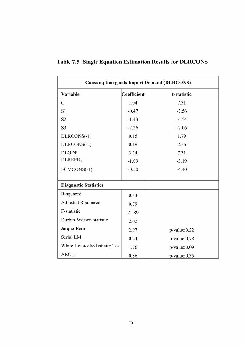
70

Table 7.5 Single Equation Estimation Results for DLRCONS

Consumption goods Import Demand (DLRCONS)

Variable Coefficient t-statistic

C 1.04 7.31

S1 -0.47 -7.56

S2 -1.43 -6.54

S3 -2.26 -7.06

DLRCONS(-1) 0.15 1.79

DLRCONS(-2) 0.19 2.36

DLGDP 3.54 7.31DLREER2 -1.09 -3.19

ECMCONS(-1) -0.50 -4.40

Diagnostic Statistics

R-squared 0.83 Adjusted R-squared 0.79 F-statistic 21.89 Durbin-Watson statistic 2.02 Jarque-Bera 2.97 p-value:0.22Serial LM 0.24 p-value:0.78White Heteroskedasticity Test 1.76 p-value:0.09ARCH 0.86 p-value:0.35