econometric analysis of large factor models analysis of large factor models jushan bai and peng...
TRANSCRIPT
Econometric Analysis of Large Factor Models
Jushan Bai∗ and Peng Wang†
August 2015
Abstract
Large factor models use a few latent factors to characterize the co-movement
of economic variables in a high dimensional data set. High dimensionality
brings challenge as well as new insight into the advancement of econometric
theory. Due to its ability to effectively summarize information in large data
sets, factor models have become increasingly popular in economics and finance.
The factors, being estimated from the high dimensional data, can help to im-
prove forecast, provide efficient instruments, control for nonlinear unobserved
heterogeneity, etc. This article reviews the theory on estimation and statistical
inference of large factor models. It also discusses important applications and
highlights future directions.
Key words: high dimensional data, factor-augmented regression, FAVAR,
number of factors, interactive effects, principal components, regularization,
Bayesian estimation
Prepared for the Annual Review of Economics
∗Department of Economics, Columbia University, New York, NY, USA. [email protected].†Department of Economics, The Hong Kong University of Science and Technology, Clear Water
Bay, Kowloon, Hong Kong. Email: [email protected].
1
Contents
1 Introduction 3
2 Large Factor Models 4
3 Determining the Number of Factors 53.1 Determining the number of dynamic factors . . . . . . . . . . . . . . 7
4 Estimating the Large Factor Model 94.1 The Principal Components Method . . . . . . . . . . . . . . . . . . . 104.2 The Generalized Principal Components . . . . . . . . . . . . . . . . . 104.3 The Maximum Likelihood Method . . . . . . . . . . . . . . . . . . . . 12
5 Factor-Augmented Regressions 13
6 Factor-Augmented Vector-Autoregression (FAVAR) 15
7 IV Estimation with Many Instrumental Variables 16
8 Structural Changes in Large Factor Models 18
9 Panel Data Models with Interactive Fixed Effects 20
10 Non-stationary Panel 2310.1 Estimating nonstationary factors . . . . . . . . . . . . . . . . . . . . 26
11 Factor Models with Structural Restrictions 2611.1 Factor Models with Block Structure . . . . . . . . . . . . . . . . . . . 2711.2 Linear Restrictions on Factor Loadings . . . . . . . . . . . . . . . . . 2811.3 SVAR and Restricted Dynamic Factor Models . . . . . . . . . . . . . 29
12 High Dimensional Covariance Estimation 30
13 Bayesian Method to Large Factor Models 31
14 Concluding Remarks 33
References 34
2
1 Introduction
With the rapid development of econometric theory and methodologies on large factor
models over the last decade, researchers are equipped with useful tools to analyze
high dimensional data sets, which become increasingly available due to advancement
of data collection technique and information technology. High dimensional data sets
in economics and finance are typically characterized by both a large cross-sectional
dimension N and a large time dimension T . Conventionally, researchers rely heav-
ily on factor models with observed factors to analyze such a data set, such as the
capital asset pricing model (CAPM) and the Fama-French factor model for asset
returns, and the affine models for bond yields. In reality, however, not all factors are
observed. This poses both theoretical and empirical challenges to researchers. The
development of modern theory on large factor models greatly broadens the scope of
factor analysis, especially when we have high dimensional data and the factors are
latent. Such a framework has helped substantially in the literature of diffusion-index
forecast, business cycle co-movement analysis, economic linkage between countries,
as well as improved causal inference through factor-augmented VAR, and providing
more efficient instrumental variables. Stock & Watson (2002) find that if they first
extract a few factors from the large data and then use the factors to augment an au-
toregressive model, the model has much better forecast performance than alternative
univariate or multivariate models. Giannoni et al. (2008) apply the factor model to
conduct now-casting, which combines data of different frequencies and forms a fore-
cast for real GDP. Bernanke et al. (2004) find that using a few factors to augment a
VAR helps to better summarize the information from different economic sectors and
produces more credible impulse responses than conventional VAR model. Boivin &
Giannoni (2006) combine factor analysis with DSGE models, providing a framework
for estimating dynamic economic models using large data set. Such a methodology
helps to mitigate the measurement error problem as well as the omitted variables
problem during estimation. Using large dynamic factor models, Ng & Ludvigson
(2009) have identified important linkages between bond returns and macroeconomic
fundamentals. Fan et al. (2011) base their high dimensional covariance estimation
on large approximate factor models, allowing sparse error covariance matrix after
taking out common factors.
Apart from its wide applications, the large factor model also brings new insight
3
to our understanding of non-stationary data. For example, the link between cointe-
gration and common trend is broken in the setup of large (N, T ). More importantly,
the common trend can be consistently estimated regardless whether individual errors
are stationary or integrated processes. That is, the number of unit roots can exceed
the number of series, yet common trends are well defined and can be alienated from
the data.
This review aims to introduce the theory and various applications of large factor
models. In particular, this review examines basic issues related to high dimensional
factors models, including determination of the number of factors, estimation of the
model via the principal components as well as the maximum likelihood method, fac-
tor augmented regression and its application, factor-augmented vector autoregression
(FAVAR), structural changes in large factor models, panel data models with interac-
tive fixed effects. This review also examines how the framework of factor models can
deal with the many instrumental variables problem, help to study non-stationarity
in panel data, incorporate restrictions to identify structural shocks, facilitate high
dimensional covariance estimation. In addition, this review provides a discussion of
the Bayesian approach to large factor models as well as its possible extensions. We
conclude with a few potential topics that deserve future research.
2 Large Factor Models
Suppose we observe xit for the i-th cross-section unit at period t. The large factor
model for xit is given by
xit = λ′iFt + eit, i = 1, ..., N, t = 1, ..., T, (1)
where the r× 1 vector of factors Ft is latent and the associated factor loadings λi is
unknown. Model (1) can also be represented in vector form,
Xt = ΛFt + et, (2)
where Xt = [x1t, ..., xNt]′ is N × 1, Λ = [λ1, ..., λN ]′ is N × r, and et = [e1t, ..., eNt]
′
is N × 1. Unlike short panel data study (large N , fixed T ) and multivariate time
series models (fixed N , large T ), the large factor model is characterized by both
large N and large T . The estimation and statistical inference are thus based on
double asymptotic theory, in which both N and T converge to infinity. Such a large
4

dimensional framework greatly expands the applicability of factor models to more
realistic economic environment. For example, weak correlations are allowed along
both the time dimension and the cross-section dimension for eit without affecting
the main properties of factor estimates. Such weak correlations in errors give rise
to what Chamberlain & Rothschild (1983) called the approximate factor structure.
Weak correlations between the factors and the idiosyncratic errors are also allowed.
The high dimensional framework also brings new insight into double asymptotics.
For example, it can be shown that it is CNT = minN1/2, T 1/2
that determines the
rate of convergence for the factor and factor loading estimates under large N and
large T .
3 Determining the Number of Factors
The number of factors is usually unknown. Alternative methods are available for esti-
mation. We will mainly focus on two types of methods. One is based on information
criteria and the other is based on the distribution of eigenvalues.
Bai & Ng (2002) treated this as a model selection problem, and proposed a
procedure which can consistently estimate the number of factors when N and T
simultaneously converge to infinity. Let λki and F kt be the principal component
estimators assuming that the number of factors is k. We may treat the sum of
squared residuals (divided by NT ) as a function of k
V (k) =1
NT
N∑i=1
T∑t=1
(xit − λk′i F k
t
)2
.
Define the following loss function
IC (k) = ln (V (k)) + k g (N, T ) ,
where the penalty function g (N, T ) satisfies two conditions: (i) g (N, T ) → 0, and
(ii) minN1/2, T 1/2
· g (N, T ) → ∞, as N, T → ∞. Define the estimator for the
number of factors as kIC = argmin0≤k≤kmax IC (k) , where kmax is the upper bound
of the true number of factors r. Then consistency can be established under standard
conditions on the factor model (Bai & Ng 2002; Bai 2003): kICp→ r, as N, T →∞.
Bai & Ng (2002) considered six formulations of the information criteria, which are
shown to have good finite sample performance. We list three here,
IC1 (k) = ln (V (k)) + k(N + T
NT
)ln( NT
N + T
),
5
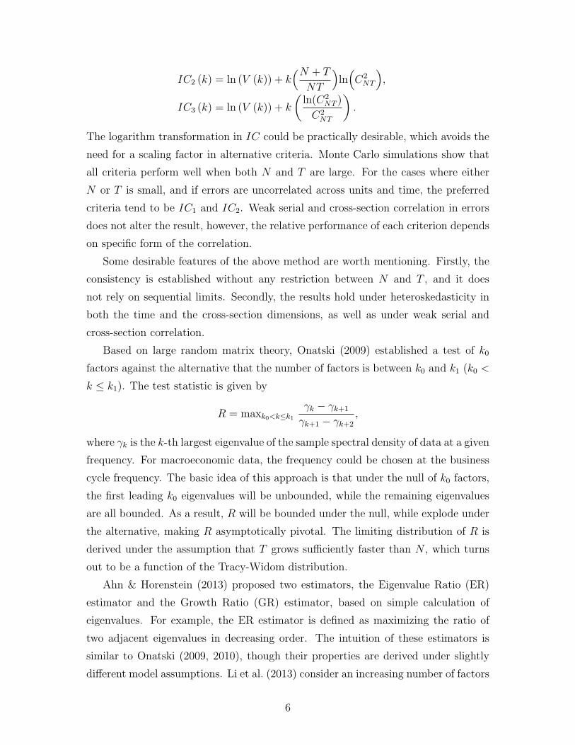
IC2 (k) = ln (V (k)) + k(N + T
NT
)ln(C2NT
),
IC3 (k) = ln (V (k)) + k
(ln(C2
NT )
C2NT
).
The logarithm transformation in IC could be practically desirable, which avoids the
need for a scaling factor in alternative criteria. Monte Carlo simulations show that
all criteria perform well when both N and T are large. For the cases where either
N or T is small, and if errors are uncorrelated across units and time, the preferred
criteria tend to be IC1 and IC2. Weak serial and cross-section correlation in errors
does not alter the result, however, the relative performance of each criterion depends
on specific form of the correlation.
Some desirable features of the above method are worth mentioning. Firstly, the
consistency is established without any restriction between N and T , and it does
not rely on sequential limits. Secondly, the results hold under heteroskedasticity in
both the time and the cross-section dimensions, as well as under weak serial and
cross-section correlation.
Based on large random matrix theory, Onatski (2009) established a test of k0
factors against the alternative that the number of factors is between k0 and k1 (k0 <
k ≤ k1). The test statistic is given by
R = maxk0<k≤k1γk − γk+1
γk+1 − γk+2
,
where γk is the k-th largest eigenvalue of the sample spectral density of data at a given
frequency. For macroeconomic data, the frequency could be chosen at the business
cycle frequency. The basic idea of this approach is that under the null of k0 factors,
the first leading k0 eigenvalues will be unbounded, while the remaining eigenvalues
are all bounded. As a result, R will be bounded under the null, while explode under
the alternative, making R asymptotically pivotal. The limiting distribution of R is
derived under the assumption that T grows sufficiently faster than N , which turns
out to be a function of the Tracy-Widom distribution.
Ahn & Horenstein (2013) proposed two estimators, the Eigenvalue Ratio (ER)
estimator and the Growth Ratio (GR) estimator, based on simple calculation of
eigenvalues. For example, the ER estimator is defined as maximizing the ratio of
two adjacent eigenvalues in decreasing order. The intuition of these estimators is
similar to Onatski (2009, 2010), though their properties are derived under slightly
different model assumptions. Li et al. (2013) consider an increasing number of factors
6
as the sample size increases.
3.1 Determining the number of dynamic factors
So far we have only considered the static factor model, where the relationship between
xit and Ft is static. The dynamic factor model considers the case in which lags of
factors also directly affect xit. The methods for static factor models can be readily
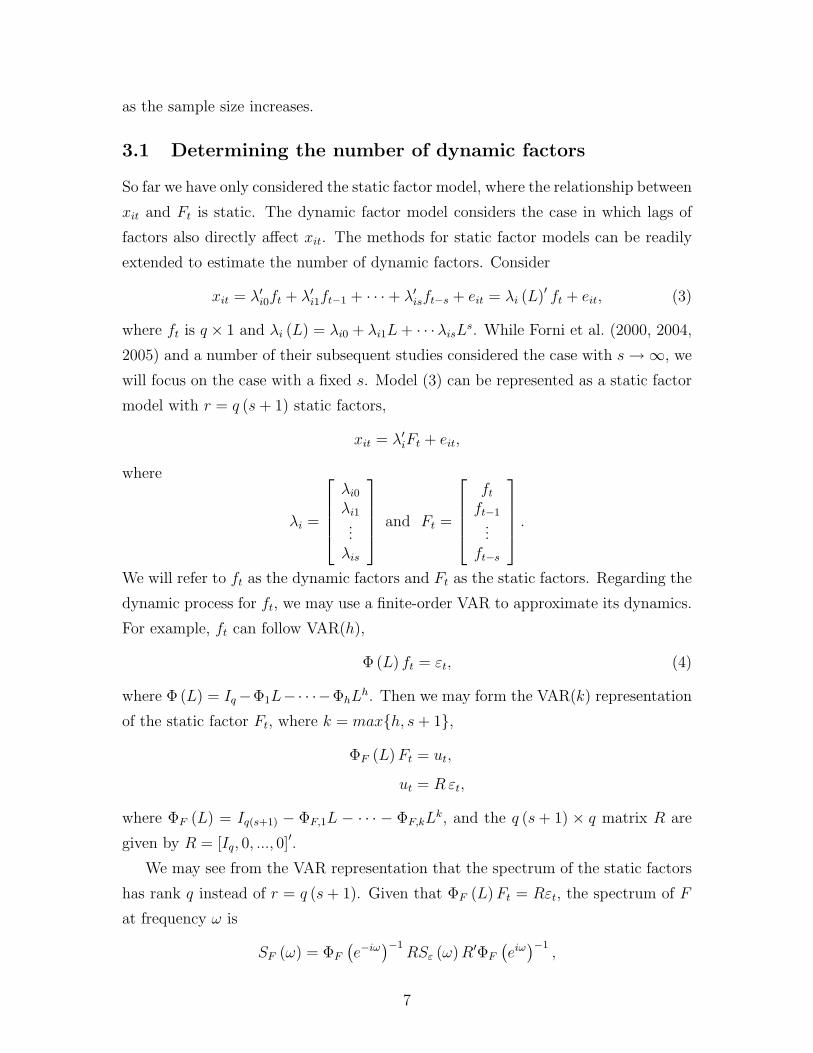
extended to estimate the number of dynamic factors. Consider
xit = λ′i0ft + λ′i1ft−1 + · · ·+ λ′isft−s + eit = λi (L)′ ft + eit, (3)
where ft is q × 1 and λi (L) = λi0 + λi1L+ · · ·λisLs. While Forni et al. (2000, 2004,
2005) and a number of their subsequent studies considered the case with s→∞, we
will focus on the case with a fixed s. Model (3) can be represented as a static factor
model with r = q (s+ 1) static factors,
xit = λ′iFt + eit,
where
λi =
λi0λi1...λis
and Ft =
ftft−1
...ft−s
.We will refer to ft as the dynamic factors and Ft as the static factors. Regarding the
dynamic process for ft, we may use a finite-order VAR to approximate its dynamics.
For example, ft can follow VAR(h),
Φ (L) ft = εt, (4)
where Φ (L) = Iq−Φ1L−· · ·−ΦhLh. Then we may form the VAR(k) representation
of the static factor Ft, where k = maxh, s+ 1,
ΦF (L)Ft = ut,
ut = Rεt,
where ΦF (L) = Iq(s+1) − ΦF,1L − · · · − ΦF,kLk, and the q (s+ 1) × q matrix R are
given by R = [Iq, 0, ..., 0]′.
We may see from the VAR representation that the spectrum of the static factors
has rank q instead of r = q (s+ 1). Given that ΦF (L)Ft = Rεt, the spectrum of F
at frequency ω is
SF (ω) = ΦF
(e−iω
)−1RSε (ω)R′ΦF
(eiω)−1
,
7
whose rank is q if Sε (ω) has rank q for |ω| ≤ π. This implies SF (ω) has only q
nonzero eigenvalues. Bai & Ng (2007) refer to q as the number of primitive shocks.
Hallin & Liska (2007) estimate the rank of this matrix to determine the number
of dynamic factors. Onatski (2009) also considers estimating q using the sample
estimates of SF (ω).
Alternatively, we may first estimate a static factor model using Bai & Ng (2002)
to obtain Ft. Next, we may estimate a VAR(p) for Ft to obtain the residuals ut. Let
Σu = 1T
∑Tt=1 utu
′t, which is semipositive definite. Note that the theoretical moments
E (utu′t) has rank q. We expect that we may estimate q using the information about
the rank of Σu. The formal procedure was provided in Bai & Ng (2007).
Using a different approach, Stock & Watson (2005) considered a richer dynamics
in error terms, and transformed the model such that the residual of the transformed
model has a static factor representation with q factors. Bai & Ng (2002)’s information
criteria can then be directly applied to estimate q.
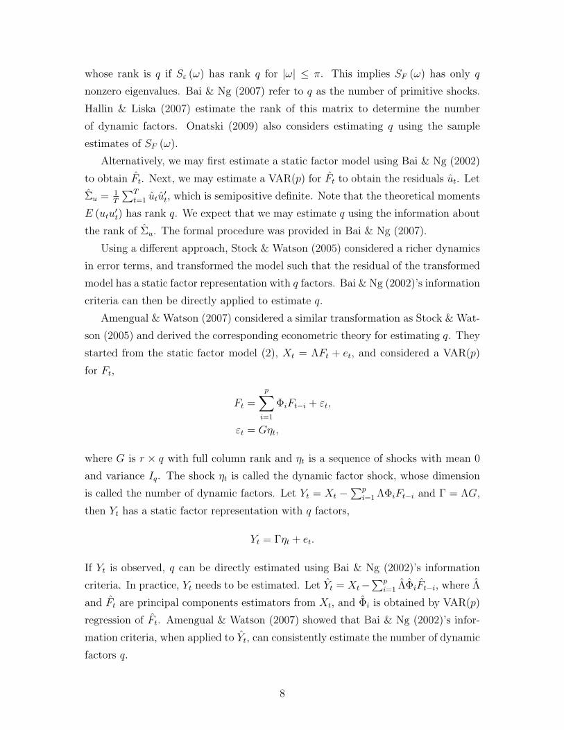
Amengual & Watson (2007) considered a similar transformation as Stock & Wat-
son (2005) and derived the corresponding econometric theory for estimating q. They
started from the static factor model (2), Xt = ΛFt + et, and considered a VAR(p)
for Ft,
Ft =
p∑i=1
ΦiFt−i + εt,
εt = Gηt,
where G is r × q with full column rank and ηt is a sequence of shocks with mean 0
and variance Iq. The shock ηt is called the dynamic factor shock, whose dimension
is called the number of dynamic factors. Let Yt = Xt −∑p
i=1 ΛΦiFt−i and Γ = ΛG,
then Yt has a static factor representation with q factors,
Yt = Γηt + et.
If Yt is observed, q can be directly estimated using Bai & Ng (2002)’s information
criteria. In practice, Yt needs to be estimated. Let Yt = Xt−∑p
i=1 ΛΦiFt−i, where Λ
and Ft are principal components estimators from Xt, and Φi is obtained by VAR(p)
regression of Ft. Amengual & Watson (2007) showed that Bai & Ng (2002)’s infor-
mation criteria, when applied to Yt, can consistently estimate the number of dynamic
factors q.
8
4 Estimating the Large Factor Model
The large factor model can be estimated using either the time-domain approach
(mainly for static factor models) or frequency-domain approach (for dynamic fac-
tors). In this section, we focus on the time domain approach. In particular, we
will mainly consider the principal component methods and the maximum likelihood
methods. Examples of the frequency domain approach is provided by Forni et al.
(2000, 2004, 2005). Throughout the remaining part, we assume the number of factors
r is known. If r is unknown, it can be replaced by k using any of the information cri-
teria discussed earlier without affecting the asymptotic properties of the estimators.
Before estimating the model, we need to impose normalizations on the factors and
factor loadings to pin down the rotational indeterminacy. This is due to the fact that
λ′iFt = (A−1λi)′(A′Ft) for any r × r full-rank matrix A. Because an arbitrary r × r
matrix has r2 degrees of freedom, we need to impose at least r2 restrictions (order
condition) to remove the indeterminacy. Let F = (F1, ..., FT )′. Three commonly
applied normalizations are PC1, PC2, and PC3 as follows.
PC1: 1TF ′F = Ir, Λ′Λ is diagonal with distinct entries.
PC2: 1TF ′F = Ir, the upper r × r block of Λ is lower triangular with nonzero
diagonal entries.
PC3: the upper r × r block of Λ is given by Ir.
PC1 is often imposed by the maximum likelihood estimation in classical factor anal-
ysis, see Anderson & Rubin (1956). PC2 is analogous to a recursive system of simul-
taneous equations. PC3 is linked with the measurement error problem such that the
first observable variable x1t is equal to the first factor f1t plus a measurement error
e1t, and the second observable variable x2t is equal to the second factor f2t plus a
measurement error e2t, and so on. Bai & Ng (2013) give a more detailed discussion
on these restrictions.
Each preceding set of normalizations yields r2 restrictions, meeting the order
condition for identification (eliminating the rotational indeterminacy). These re-
strictions also satisfy the rank condition for identification (Bai & Wang 2014). The
common components λ′iFt have no rotational indeterminacy, and are identifiable
without restrictions.
9
4.1 The Principal Components Method
The principal components estimators for factors and factor loadings can be treated
as outcomes of a least squares problem under normalization PC1. Estimators under
normalizations PC2 and PC3 can be obtained by properly rotating the principal
components estimators. Consider minimizing the sum of squares residuals under
PC1,N∑i=1
T∑t=1
(xit − λ′iFt)2
= tr[(X − FΛ′)(X − FΛ′)′]
where X = (X1, X2, ..., XT )′, a T ×N data matrix. It can be shown that F is given
by the the first r leading eigenvectors1 of XX ′ multiplied by T 1/2, and Λ = X ′F /T ;
see, for example, Connor & Korajczyk (1986) and Stock & Watson (1998). Bai
(2003) studied the asymptotic properties under large N and T . Under the general
condition√N/T → 0,
√N(Ft−HF 0
t )d→ N (0, VF ), where H is the rotation matrix,
F 0t is the true factor, and VF is the estimable asymptotic variance. By symmetry,
when√T/N → 0, λi is also asymptotically normal. Specifically,
√T (λi−H ′−1λ0
i )d→
N (0, VΛ), for some VΛ > 0. The standard principal components estimates can be
rotated to obtain estimates satisfying PC2 or PC3. The limiting distributions under
PC2 and PC3 are obtained by Bai & Ng (2013). As for the common component
λ′iFt, its limiting distribution requires no restriction on the relationship between N
and T , which is always normal. In particular, there exists a sequence of bNT =
minN1/2, T 1/2 such that
bNT
(λ′iFt − λ′iFt
)d→ N (0, 1) , as N, T →∞.
So the convergence rate for the estimated common components is minN1/2, T 1/2.This is the best rate possible.
4.2 The Generalized Principal Components
The principal components estimator is a least squraes estimator (OLS) and is efficient
if Σe is a scalar multiple of an N×N identity matrix, that is, Σe = cIN for a constant
c > 0. This is hardly true in practice, therefore a generalized least squares (GLS)
will give more efficient estimation. Consider the GLS objective function, assuming
Σe is known,
1If there is an intercept in the model Xt = µ + Λft + et, then the matrix X is replaced by itsdemeaned version X − (1, 1, ..., 1)⊗ X = (X1 − X,X2 − X, ..., XT − X), where X = T−1
∑Tt=1Xt.
10
minΛ,F
tr[(X − FΛ′)Σ−1
e (X − FΛ′)′]
Then the solution for F is given by the first r eigenvectors of the matrix XΣ−1e X ′,
multiplied by T 1/2, and the solution for Λ is equal to X ′F /T . The latter has the
same expression as the standard principal components estimator.
This is the generalized principal components estimator (GPCE) considered by
Choi (2012). He showed that the GPCE of the common component has smaller
variance than the principal component estimator. Using the GPCE-based factor
estimates will also produce smaller variance of the forecasting error.
In practice Σe is unknown, and needs to be replaced by an estimate. The usual
covariance matrix estimator 1T
∑Tt=1 ete
′t based on the standard principal components
residuals et is not applicable since it is not a full rank matrix, regardless of the
magnitude of N and T . Even if every element of Σe can be consistently estimated by
some way and the resulting estimator Σe is of full rank, the GPCE is not necessarily
more accurate than the standard PC estimator. Unlike standard inference with
a finite dimensional weighting matrix (such as GMM), a mere consistency of Σe
is insufficient to obtain the limiting distribution of the GPCE. Even an optimally
estimated Σe in the sense of Cai & Zhou (2012) is not enough to establish the
asymptotically equivalence between the feasible and infeasible estimators. So the
high dimensionality of Σe makes a fundamental difference in terms of inference. Bai
& Liao (2013) show that the true matrix Σe has to be sparse and its estimates
should take into account the sparsity assumption. Sparsity does not require many
zero elements, but many elements must be sufficiently small. Under the sparsity
assumption, a shrinkage estimator of Σe (for example, a hard thresholding method
based on the residuals from the standard PC method) will give a consistent estimation
of Σe. Bai & Liao (2013) derive the conditions under which the estimated Σe can be
treated as known.
Other related methods include Breitung & Tenhofen (2011), who proposed a
two-step estimation procedure, which allows for heteroskedastic (diagonal Σe) and
serially correlated errors. They showed that the feasible two-step estimator has
the same limiting distribution as the GLS estimator. In finite samples, the GLS
estimators tend to be more efficient than the usual principal components estimators.
An iterated version of the two-step estimation method is also proposed, which is
shown to further improve efficiency in finite sample.
11
4.3 The Maximum Likelihood Method
For the factor model Xt = µ + Λft + et, under the assumption that et is iid normal
N(0,Σe) and ft is iid normal N(0, Ir), then Xt is normal N(µ,Ω), where Ω = ΛΛ′ +
Σe, it follows that the likelihood function is
L(Λ,Σe) = − 1
Nlog |ΛΛ′ + Σe| −
1
Ntr(S(ΛΛ′ + Σe)
−1)
where S = 1T
∑Tt=1(Xt− X)(Xt− X)′ is the sample covariance matrix. The classical
inferential theory of the MLE is developed assuming N is fixed, and the sample size
T goes to infinity, see Anderson (2013), Anderson & Rubin (1956), and Lawley &
Maxwell (1971). The basic assumption in classical factor analysis is that√T (S−Ω) is
asymptotically normal. This basic premise does not hold when N also goes to infinity.
A new approach is required to obtain consistency and the limiting distribution under
large N . Bai & Li (2012a) derive the inferential theory assuming Σe is diagonal under
various identification restrictions.
Normality assumption is inessential. The preceding likelihood is considered as the
quasi-likelihood under non-normality. It is useful to point out that MLE is consistent
even if N is fixed because the fixed N case falls within the classical framework. In
contrast, the principal components method is inconsistent under fixed N unless Σe
is proportional to an identity matrix. The GPCE is hardly consistent when using
residuals to estimate Σe because the residual eit = xit− µi− λ′ift is not consistent for
eit. This follows because ft is not consistent for ft under fixed N . The MLE treats
Σe as a parameter, which is jointly estimated with Λ. The MLE does not rely on
residuals to estimate Σe.
The maximum likelihood estimation for non-diagonal Σe is considered by Bai
& Liao (2012). They assume Σe is sparse and use the regularization method to
jointly estimate Λ and Σe. Consistency is established for the estimated Λ and Σe,
but the limiting distributions remain unsolved, though the limiting distributions are
conjectured to be the same as the two-step feasible GLS estimator in Bai & Liao
(2013) under large N and T .
Given the MLE for Λ and Σe, the estimator for ft is ft = (Λ′Σ−1e Λ)−1Λ′Σ−1
e (Xt−X) for t = 1, 2, ..., T . This is a feasible GLS estimator of ft in the model Xt =
µ+Λft+et. The estimated factor loadings have the same asymptotic distributions for
the three different estimation methods (PC, GPCE, MLE) under large N and large
T , But the estimated factors are more efficient under GPCE and MLE than standard
12
PC (see Choi 2010; Bai & Li 2012; Bai & Liao 2013). If time series heteroskedasticity
is of more concern, and especially when T is relatively small, then the role of F and
Λ (also T and N) should be switched. Bai & Li (2012) considered the likelihood
function for this setting.
The preceding discussion assumes the factors ft are iid. Doz et al. (2011, 2012)
explicitly considered a finite-order VAR specification for ft, and then proposed a two-
step method or a quasi-maximum likelihood estimation procedure. The method is
similar to the maximum likelihood estimation of a linear state space model. The main
difference is that they initialize the estimation by using properly rotated principal
component estimators. The factor estimates are obtained as either the Kalman
filter or the Kalman smoother. They showed that estimation under independent
Gaussian errors still lead to consistent estimators for the large approximate factor
model, even when the true model has cross-sectional and time series correlation in the
idiosyncratic errors. Bai & Li (2012b) studied related issues for dynamic factors and
cross-sectionally and serially correlated errors estimated by the maximum likelihood
method.
5 Factor-Augmented Regressions
One of the popular applications of large factor model is the factor-augmented regres-
sions. For example, Stock & Watson (1999, 2002a) added a single factor to standard
univariate autoregressive models and found that they provided the most accurate
forecasts of macroeconomic time series such as inflation and industrial production
among a large set of models. Bai & Ng (2006) developed the econometric theory for
such factor-augmented regressions so that inference can be conducted.
Consider the following forecasting model for yt,
yt+h = α′Ft + β′Wt + εt+h, (5)
where Wt is the vector of a small number of observables including lags of yt, and Ft is
unobservable. Suppose there is a large number of series xit, i = 1, ..., N , t = 1, ..., T ,
which has a large factor representation as (1),
xit = λ′iFt + eit.
When yt is a scalar, (5) and (1) become the diffusion index forecasting model of
Stock & Watson (2002b). Clearly, each xit is a noisy predictor for yt+h. Because Ft
13
is latent, the conventional mean-squared optimal prediction of yt+h is not feasible.
Alternatively, consider estimating (1) by the method of principal components to
obtain Ft, which is a consistent estimator for H ′Ft for some rotation matrix H,
and then regress yt+h on Ft and Wt to obtain α and β. The feasible prediction for
yT+h|T ≡ E (yT+h|ΩT ), where ΩT = [FT ,WT , FT−1,WT−1, ...], is given by
yT+h|T = α′FT + βWT .
Let δ ≡ (α′H−1, β′)′and εT+h|T ≡ yT+h−yT+h|T , Bai & Ng (2006) showed that when
N is large relative to T (i.e.,√T/N → 0), δ will be
√T -consistent and asymptoti-
cally normal. yT+h|T and εT+h|T are minN1/2, T 1/2
-consistent and asymptotically
normal. For all cases, inference needs to take into account the estimated factors,
except for the special case T/N → 0. In particular, under standard assumptions for
large approximate factor model as in Bai & Ng (2002), when√T/N → 0, we have
δ − δ d→ N (0,Σδ) .
Let zt = [F ′t ,W′t ]′, zt =
[F ′t ,W
′t
]′, and εt+h = yt+h − yt+h|t, a heteroskedasticity-
consistent estimator for Σδ is given by
Σδ =
(1
T
T−h∑t=1
ztz′t
)−1(1
T
T−h∑t=1
ε2t+hztz
′t
)(1
T
T−h∑t=1
ztz′t
)−1
.
The key requirement of the theory is√T/N → 0, which puts discipline on when
estimated factors can be applied in the diffusion index forecasting models as well as
the FAVAR to be considered in the next section.
If in addition, we assume√N/T → 0, then
yT+h|T − yT+h|T√var
(yT+h|T
) d→ N (0, 1) ,
where
var(yT+h|T
)=
1
Nz′TAvar
(δ)zT +
1
Nα′Avar
(FT
)α.
An estimator for Avar(FT
)is provided in Bai (2003). A notable feature of the
limiting distribution of the forecast is that the overall convergence rate is given by
minN1/2, T 1/2
. Given that εT+h = yT+h|T − yT+h = yT+h|T − yT+h|T + εT+h, if we
further assume that εt is normal with variance σ2ε , then the forecasting error also
becomes approximately normal
εT+h ∼ N(0, σ2
ε + var(yT+h|T
)),
so that confidence intervals can be constructed for the forecasts.
14
6 Factor-Augmented Vector-Autoregression (FAVAR)
VAR models have been widely applied in macroeconomic analysis. A central question
of using VAR is how to identify structural shocks, which in turn depends on what
variables to include in the VAR system. A small VAR usually cannot fully capture
the structural shocks. In the meantime, including more variables in the VAR system
could be problematic due to either the degree of freedom problem or the variable
selection problem. It has been a challenging job to determine which variables to be
included in the system. There have been a number of ways to overcome such diffi-
culties, such as Bayesian VAR, initially considered by Doan et al. (1984), Litterman
(1986), and Sims (1993), and Global VAR of Pesaran et al. (2004). This section
will focus on another popular solution, the factor-augmented vector autoregressions
(FAVAR), originally proposed by Bernanke et al. (2005). The FAVAR assumes that
a large number of economic variables are driven by a small VAR, which can in-
clude both latent and observed variables. The dimension of structural shocks can be
estimated instead of being assumed to be known and fixed.
Consider the case where both the unobserved factors Ft and the observed factors
Wt affect a large number of observed variables xit,
xit = λ′iFt + γ′iWt + eit, (6)
and that the vector Ht = [F ′t ,W′t ]′ follows a VAR of finite order,
Φ (L)Ht = ut.
Bernanke et al. (2005) proposed two ways to analyze the FAVAR. The first is based
on a two-step principal components method, where in the first step method of prin-
cipal components is employed to form estimates of the space spanned by both Ft and
Wt. In the second step, various identification schemes can be applied to obtain esti-
mates of latent factors Ft, which is treated as observed when conduct VAR analysis
of[F ′t ,W
′t
]′. Bai et al. (2015) show that, under suitable identification conditions,
inferential theory can be developed for such a two-step estimator, which differs from
a standard large factor model. Confidence bands for the impulse responses can be
readily constructed using the theory therein. The second method involves a one-step
likelihood approach, implemented by Gibbs sampling, which leads to joint estima-
tion of both the latent factors and the impulse responses. The two methods can be
complement of each other, with the first one being computationally simple, and the
15
second providing possibly better inference in finite sample at the cost of increased
computational cost.
A useful feature of the FAVAR is that the impulse response function of all vari-
ables to the fundamental shocks can be readily calculated. For example, the impulse
response of the observable xi,t+h with respect to the structural shock ut is,
∂xi,t+h∂ut
= (λ′i, γ′i)Ch, (7)
where Ch is the coefficient matrix for ut−h in the vector moving average (VMA)
representation of Ht,
Ht = Φ (L)−1 ut = C0ut + C1ut−1 + C2ut−2 + · · · .
Theory of estimation and inference for (7) is provided in Bai et al. (2015). Forni
et al. (2009) explored the structural implication of the factors and developed the
corresponding econometric theory. Stock and Watson (2010) provide a survey on the
application of dynamic factor models.
7 IV Estimation with Many Instrumental Vari-
ables
The IV method is fundamental in econometrics practice. It is useful when one
or more explanatory variables are correlated with the error terms in a regression
model, known as endogenous regressors. In this case, standard methods such as
the OLS are inconsistent. With the availability of instrumental variables, which
are correlated with regressors but uncorrelated with errors, consistent estimation is
achievable. Consider a standard setup
yt = x′tβ + ut, t = 1, 2, ..., T, (8)
where xt is correlated with the error term ut. Suppose there are N instrumental
variables labeled as zit for i = 1, 2, ..., N . Consider the two-stage least squares (2SLS),
a special IV method. In the first stage, the endogenous regressor xt is regressed on
the IVs
xt = c0 + c1z1t + · · ·+ cNzNt + ηt (9)
the fitted value xt is used as the regressor in the second stage, and the resulting
estimator is consistent for β for a small N . It is known that for large N , the 2SLS
16
can be severely biased. In fact, if N ≥ T , then xt ≡ xt, and the 2SLS method
coincides with the OLS, which is inconsistent. The problem lies in the overfitting in
the first stage regression. The theory of many instruments bias has been extensively
studied in the econometric literature, for example, Hansen et al. (2008) and Hausman
et al. (2010). Within the GMM context, inaccurate estimation of a high dimensional
optimal weighting matrix is not the cause for many-moments bias. Bai and Ng
(2010) show that even if the true optimal weighting matrix is used, inconsistency is
still obtained under large number of moments. In fact, with many moments, sparse
weighting matrix such as an identity matrix will give consistent estimation, as is
shown by Meng et al. (2011).
One solution for the many IV problem is to assume that many of the coefficients
in (9) are zero (sparse) so that regularization method such as LASSO can be used
in the first stage regression. Penalization prevents over fitting, and picks up the
relevant instruments (non-zero coefficients). These methods are considered by Ng
& Bai (2009) and Belloni et al. (2012). In fact, any machine learning method that
prevents in-sample overfitting in the first stage regression will work.
The principal components method is an alternative solution, and can be more
advantageous than the regularization method (Bai & Ng 2010; Kapetanios & Mar-
cellino 2010). It is well known that the PC method is that of dimension reduction.
The principal components are linear combinations of z1t, ..., zNt. The high dimension
of the IVs can be reduced into a smaller dimension via the PC method. If z1t, ..., zNT
are valid instruments, then any linear combination is also a valid IV, so are the prin-
cipal components. Interestingly, the PC method does not require the z’s to be valid
IVs to begin with. Suppose that both the regressors xt and z1t, ..., zNt are driven by
some common factors Ft such that
xt = φ′Ft + ext,
zit = λ′iFt + et.
Provided that the common shocks Ft are uncorrelated with errors ut in equation (8),
then Ft is a valid IV because Ft also drives xt. Although Ft is unobservable, it can
be estimated from zit via the principal components. Even though the et can be
correlated with ut, so that zit are not valid IV, the principal components are valid
IVs. This is the advantage of principal components method. The example in Meng
et al. (2011) is instructive. Consider estimating the beta of an asset with respect
17
to the market portfolio, which is unobservable. The market index, as a proxy, is
measured with errors. But other assets’ returns can be used as instrument variables
because all assets’s returns are linked with the market portfolio. So there exists a
large number of instruments. Each individual asset can be a weak IV because the
idiosyncratic returns can be large. But the principal components method will wash
out the idiosyncratic errors, giving rise to a more effective IV.
The preceding setup can be extended into panel data with endogenous regressors:
yit = x′itβ + uit, t = 1, 2, ..., T ; i = 1, 2, ..., N,
where xit are correlated with the errors uit. Suppose that xit are driven by the
common shocks Ft such that
xit = γ′iFt + eit
Provided that the common components cit = γ′iFt are uncorrelated with uit, outside
instrumental variables are not needed. We can extract the common components cit
via the principal components estimation of γi and Ft to form cit = γ′iFt, and use cit
as IV. This method is considered by Bai & Ng (2010).
8 Structural Changes in Large Factor Models
In a lot of economic applications, researchers have to be cautious about the potential
structural changes in the high dimensional data sets. Parameter instability has been
a pervasive phenomenon in time series data (Stock & Watson 1996). Such instability
could be due to technological changes, preference shifts of consumers, and policy
regimes switching. Banerjee & Marcellino (2008) and Yamamoto (2014) provide
simulation and empirical evidence that the forecasts based on estimated factors will
be less accurate if the structural break in the factor loading matrix is ignored. In
addition, evolution of an economy might introduce new factors, while conventional
factors might phase out. Econometric analysis of the structural change in large
factor models is challenging because the factors are unobserved and factor loadings
have to be estimated. Structural change can happen to either the factor loadings or
the dynamic process of factors or both. Most theoretical challenge comes from the
break in factor loadings, given that factors can be consistently estimated by principal
components even if their dynamic process is subject to a break while factor loadings
are time-invariant. In this section, we will focus on the breaks in factor loadings.
18

Consider a time-varying version of (2),
Xt = ΛtFt + et,
where the time-varying loading matrix Λt might assume different forms. Bates et al.
(2013) considered the following dynamic equation
Λt = Λ0 + hNT ξt,
where hNT is a deterministic scalar that depends on (N, T ), and ξt is N×r stochastic
process. Three examples are considered for ξt: white noise, random walk, and single
break. Bates et al. (2013) then established conditions under which the changes in the
loading matrix can be ignored in the estimation of factors. Intuitively, the estimation
and inference of the factor estimates is not affected if the size of the break is small
enough. If the size of the break is large, however, the principal components factor
estimators will be inconsistent.
Recent years have witnessed fast development in this area. Tests for structural
changes in factor loadings of a specific variable have been derived by Stock & Watson
(2008), Breitung & Eickmeier (2011), and Tanaka & Yamamoto (2015). Chen et al.
(2014) and Han & Inoue (2014) studied tests for structural changes in the overall
factor loading matrix. Corradi & Swanson (2014) constructed joint tests for breaks in
factor loadings and coefficients in factor-augmented regressions. Cheng et al. (2015)
considered the determination of break date and introduced the shrinkage estimation
method for factor models in the presence of structural changes. Current studies
have not considered the case where break dates are possibly heterogeneous across
variables and the number of break dates might increase with the sample size. It
would be interesting to study the properties of the principal components estimators
and the power of the structural change tests under such scenarios.
Another branch of methods considers Markov regime switching in factor loadings
(Kim & Nelson 1999). The likelihood function can be constructed using various fil-
ters. Then one may use either maximum likelihood or Bayesian method to estimate
factor loadings in different regimes, the regime probabilities, as well as the latent fac-
tors. Del Negro & Otrok (2008) developed a dynamic factor model with time-varying
factor loadings and stochastic volatility in both the latent factors and idiosyncratic
components. A Bayesian algorithm is developed to estimate the model, which is
employed to study the evolution of international business cycles. The theoretical
properties of such models remain to be studied under the large N large T setup.
19
9 Panel Data Models with Interactive Fixed Ef-
fects
There has been growing study in panel data models with interactive fixed effects.
Conventional methods assumes additive individual fixed effects and time fixed effects.
The interactive fixed effects allows possible multiplicative effects. Such a methodol-
ogy has important theoretical and empirical relevance. Consider the following large
N large T panel data model
yit = X ′itβ + uit,
uit = λ′iFt + εit. (10)
We observe yit and Xit, but do not observe λi, Ft, and εit. The coefficient of interest
is β. Note that such model nests conventional fixed effects panel data models as
special cases due to the following simple transformation
yit = X ′itβ + αi + ξt + εit
= X ′itβ + λ′iFt + εit,
where λi = [1, αi]′ and Ft = [ξt, 1]′. In general, the interactive fixed effects allow
a much richer form of unobserved heterogeneity. For example, Ft can represent a
vector of macroeconomic common shocks and λi captures individual i’s heterogeneous
response to such shocks.
The theoretic framework of Bai (2009) allows Xit to be correlated with λi, Ft, or
both. Under the framework of large N and large T , we may estimate the model by
minimizing a least squares objective function
SSR (β, F,Λ) =N∑i=1
(Yi −Xiβ − Fλi)′ (Yi −Xiβ − Fλi)
s.t. F ′F/T = Ir, Λ′Λ is diagonal.
Although no closed-form solution is available, the estimators can be obtained by iter-
ations. Firstly, consider some initial values β(0), such as least squares estimators from
regressing Yi on Xi. Then perform principal component analysis for the pseudo-data
Yi −Xiβ(0) to obtain F (1) and Λ(1). Next, regress Yi − F (1)λ
(1)i on Xi to obtain β(1).
Iterate such steps until convergence is achieved. Bai (2009) showed that the resulting
estimator β is√NT -consistent. Given such results, the limiting distributions for F
20
and Λ are the same as in Bai (2003) due to their slower convergence rates. The
limiting distribution for β depends on specific assumptions on the error term εit as
well as on the ratio T/N . If T/N → 0, then the limiting distribution of β will be
centered around zero, given that E (εitεjs) = 0 for t 6= s, and E (εitεjt) = σij for all
i, j, t.
On the other hand, if N and T are comparable such that T/N → ρ > 0, then the
limiting distribution will not be centered around zero, which poses a challenge for
inference. Bai (2009) provided a bias-corrected estimator for β, whose limiting dis-
tribution is centered around zero. In particular, the bias-corrected estimator allows
for heteroskedasticity across both N and T . Letˆβ be the bias-corrected estimator,
assume that T/N2 → 0 and N/T 2 → 0, E (ε2it) = σ2
it, and E (εitεjs) = 0 for i 6= j
and t 6= s, then√NT
(ˆβ − β
)d→ N (0,Σβ) ,
where a consistent estimator for Σβ is also available in Bai (2009).
Ahn et al. (2001, 2013) studied model (10) under large N but fixed T . They em-
ployed the GMM method that applies moments of zero correlation and homoskedas-
ticity. Moon & Weidner (2014) considered the same model as (10), but allowed
lagged dependent variable as regressors. They devised a quadratic approximation
of the profile objective function to show the asymptotic theory for the least square
estimators and various test statistics. Moon & Weidner (2015) further extended
their study by allowing unknown number of factors. They showed that the limiting
distribution of the least square estimator is not affected by the number of factors
used in the estimation, as long as this number is no smaller than the true number of
factors. Lu & Su (2015) proposed the method of adaptive group LASSO (least ab-
solute shrinkage and selection operator), which can simultaneously select the proper
regressors and determine the number of factors.
Pesaran (2006) considered a slightly different setup with individual-specific slopes,
yit = α′idt +X ′itβi + uit, (11)
uit = λ′iFt + εit,
where dt is observed common effects such as seasonal dummies. The regressor Xit
is allowed to be correlated with both λi and Ft, which makes direct OLS incon-
sistent. The unobserved factors and the individual-specific errors are allowed to
follow arbitrary stationary processes. Instead of estimating the factors and factor
21
loadings, Pesaran (2006) considered an auxiliary OLS regression. The proposed com-
mon correlated effects estimator (CCE) can be obtained by augmenting the model
with additional regressors, which are the cross sectional averages of the dependent
and independent variables, in an attempt to control for the common factors. Define
zit = [yit, X′it]′ as the collection of individual-specific observations. Consider weighted
average of zit as
zωt =N∑i=1
ωizit,
with the weights that satisfy some very general conditions. For example, we may
choose ωi = 1/N . Pesaran (2006) showed that the individual slope βi can be con-
sistently estimated through the following OLS regression of yit on dt, Xit, and zωt
under the large N and large T framework,
yit = α′idt +X ′itβi + z′ωtγi + εit. (12)
In the same time, the mean β = E (βi) can be consistently estimated by a pooled
regression of yit on dt, Xit, and zωt as long as N tends to infinity, regardless of large
or small T ,
yit = α′idt +X ′itβ + z′ωtγ + vit. (13)
Alternatively, the mean β can also be consistently estimated by taking simple average
of individual estimators from (12), βMG = 1N
∑Ni=1 β
CCEi . Asymptotic normality for
such CCE estimators can also be established and help conduct inference. A clear
advantage of the CCE method is that the number of unobserved factors need not
be estimated. In fact, the method is valid with a single or multiple unobserved
factors and does not require the number of factors to be smaller than the number of
observed cross-section averages. In addition, CCE is easy to compute as an outcome
of OLS and no iteration is needed. Desirable small sample properties of CCE are
also demonstrated.
Heterogenous panel models with interactive effects are also studied by Ando & Bai
(2014), where the number of regressors can be large and the regularization method
is used to select relevant regressors. Su & Chen (2013) and Ando & Bai (2015)
provided a formal test for homogenous coefficients in model (11).
The maximum likelihood estimation of model (10) is studied by Bai & Li (2014).
They consider the case in which Xit also follows a factor structure and is jointly
modeled.
22
10 Non-stationary Panel
Other important topics includes the application of large factor models in non-stationary
panel data, estimation and inference of dynamic factor models.
For non-stationary analysis, large factor model brings new prospective for the
tests of unit roots. Consider the following data generating process for xit,
xit = ci + βit+ λ′iFt + eit, (14)
(1− L)Ft = C (L)ut,
(1− ρiL) eit = Di (L) εit,
where C (L) and Di (L) are polynomials of lag operators. The r × 1 factor Ft has
r0 stationary factors and r1 I (1) components or common trends (r = r0 + r1).
The idiosyncratic errors eit could be either I (1) or I (0), depending on whether
ρi = 1 or |ρi| < 1. The Panel Analysis of Nonstationarity in the Idiosyncratic and
Common components (PANIC) by Bai & Ng (2004) develops an econometric theory
for determining r1 and testing ρi = 1 when neither Ft nor eit is observed. Model
(14) has many important features that are of both theoretical interests and empirical
relevance. For example, let xit denote the real output for country i. Then it may be
determined by the global common trend F1t, the global cyclical component F2t, and
an idiosyncratic component eit that could be either I(0) or I(1). PANIC provides
a framework for the estimation and statistical inference for such components, which
are all unobserved. While the conventional nonstationarity analysis looks at unit
root in xit only, PANIC further explores whether possible unit roots are coming
from common factors or idiosyncratic components or both. Another very important
feature of PANIC is that it allows weak cross-section correlation in idiosyncratic
errors.
The initial steps of PANIC include transformations of the data so that the de-
terministic trend part is removed, and then proceed with principal component anal-
ysis. In the case of no linear trend (βi = 0 for all i), a simple first differencing
will suffice. We will proceed with the example with a linear trend (βi 6= 0 for
some i). Let ∆xit = xit − xi,t−1, ∆xi = 1T−1
∑Tt=2 ∆xit, ∆ei = 1
T−1
∑Tt=2 ∆eit,
∆F = 1T−1
∑Tt=2 ∆Ft. After first differencing and remove the time average, model
(14) becomes
∆xit −∆xi = λ′ift + ∆eit −∆ei, (15)
23
where ft = ∆Ft − ∆F . Let λi and ft be the principal components estimators of
(15). Let zit = ∆xit − ∆xi − λ′ift, eit =∑t
s=2 zit, and Ft =∑t
s=2 ft. Then test
statistics for unit root in eit and Ft can be constructed based on the estimates eit and
Ft. Let ADF τe (i) denote the Augmented Dickey-Fuller test using eit. The limiting
distributions and critical values are provided in Bai & Ng (2004).
A few important properties of PANIC are worth mentioning. First, the test on
idiosyncratic errors eit can be conducted without knowing whether the factors are
I (1) or I (0). Likewise, the test on factors is valid regardless whether eit is I (1) or
I (0). Last but not the least, the test on eit is valid no matter whether ejt (j 6= i) is
I (1) or I (0). In fact, the limiting distribution of ADF τe (i) does not depend on the
common factors. This helps to construct pooled panel unit root tests, which have
improved power as compared to univariate unit root tests.
The literature on panel unit root tests has been growing fast. The early test
in Quah (1994) requires strong homogeneous cross-sectional properties. Later tests
of Levin et al. (2002) and Im et al. (2003) allow for heterogeneous intercepts and
slopes, but assume cross-sectional independence. Such an assumption is restrictive,
and tend to over reject the null hypothesis when violated. O’Connell (1998) provides
a GLS solution to this problem under fixed N . However, such a solution does not
apply when N tends to ∞, especially for the case where N > T . The method of
PANIC allows strong cross-section correlation due to common factors, as is widely
observed in economic data, as well as weak cross-section correlation in eit. In the
same time, it allows heterogeneous intercepts and slopes. If we further assume that
the idiosyncratic errors eit are independent across i, and consider testing H0 : ρi = 1
for all i, against H1 : ρi < 1 for some i, a pool test statistic can be readily constructed.
Let pτe (i) be the p-value associated with ADF τe (i). Then
P τe =−2∑N
i=1 logpτe (i)− 2N√4N
d→ N (0, 1) .
The pooled test of the idiosyncratic errors can also be seen as a panel test of no
cointegration, as the null hypothesis that ρi = 1 for all i holds only if no stationary
combination of xit can be formed.
Alternative methods to PANIC include Kapetanios et al. (2011), who derived the
theoretical properties of the common correlated effects estimator (CCE) of Pesaran
(2006) for panel regression with nonstationary common factors. The model slightly
differs from PANIC in the sense that individual slopes can be studied. For example,
24
they consider
yit = α′idt +X ′itβi + λ′iFt + εit,
and the parameter of interest is βi. Another difference is that the individual error
εit is assumed to be stationary. They show that the cross-sectional-average-based
CCE estimator is robust to a wide variety of data generation processes, and not just
restricted to stationary panel regression. Similar to Pesaran (2006), the method does
not require the knowledge of the number of unobserved factors. The only requirement
is that the number of unobserved factors remains fixed as the sample size grows. The
main results of Pesaran (2006) continue to hold in the case of nonstationary panel. It
is also shown that the CCE has lower biases than the alternative estimation methods.
While Kapetanios et al. (2011) does not focus on testing panel unit roots, the
main idea of CCE can be applied for such a purpose. For a given individual i,
Pesaran (2007) augments the Dickey-Fuller (DF) regression of yit with cross-section
averages yt−1 = 1N
∑Ni=1 yi,t−1 and ∆yt−1 = yt−1− yt−2. Such auxiliary regressors help
to take account of cross-section dependence in error terms. The regression can be
further augmented with ∆yi,t−s and ∆yt−s for s = 1, 2, ..., to handle possible serial
correlation in the errors. The resulting augmented DF statistic is referred to as
CADF statistic for individual i. The panel unit root test statistic is then computed
as the average, CADF = 1N
∑Ni=1CADFi. Due to correlation among CADFi, the
limiting distribution of CADF is non-normal. The CADF is shown to have good
finite sample performance while only a single common factor is present. However, it
shows size distortions in case of multiple factors.
Pesaran et al. (2013) extends Pesaran (2007) to the case with multiple common
factors. They proposed a new panel unit root test based on a simple average of cross-
sectionally augmented Sargan-Bhargava statistics (CSB). The basic idea is similar
to CCE of Pesaran (2006), which exploits information of the unobserved factors that
are shared by all observed time series. They showed that the limit distribution of the
tests is free from nuisance parameters given that the number of factors is no larger
than the number of observed cross-section averages. The new test has the advantage
that it does not require all the factors to be strong in the sense of Bailey et al. (2012).
Monte Carlo simulations show that the proposed tests have the correct size for all
combinations of N and T considered, with power rising with N and T .
25
10.1 Estimating nonstationary factors
Studies in Bai & Ng (2002) and Bai (2003) assume the errors are I (0). The method
of PANIC allows estimating factors under either I (1) or I (0) errors. To convey the
main idea, consider the case without linear trend (βi = 0 for all i). The factor model
after differencing is
∆xit = λ′i∆Ft + ∆eit.
If eit is I (1), ∆eit is I (0). If eit is I (0), then ∆eit is still I (0), though over-differenced.
Under the assumption of weak cross-section and serial correlation in ∆eit, consistent
estimators for ∆Ft can be readily constructed.
It is worth mentioning that when eit is I(0), estimating the original level equation
already provides a consistent estimator for Ft (Bai & Ng 2002; Bai 2003). Although
such estimators could be more efficient than the ones based on the differenced equa-
tions, they are not consistent when eit is I(1). An advantage of estimation based on
differenced equation is that the factors in levels can still be consistently estimated.
Define Ft =∑t
s=2 ∆F s and eit =∑t
s=2 ∆eis. Bai & Ng (2004) shows that Ft and eit
are consistent for Ft and eit respectively. In particular, uniform convergence can be
established (up to a location shift factor)2,
max1 ≤ t ≤ T
∥∥∥Ft −HFt +HF1
∥∥∥ = Op
(T 1/2N−1/2
)+Op
(T−1/4
).
Such a result implies that even if each cross-section equation is a spurious regression,
the common stochastic trends are well defined and can be consistently estimated,
given their existence, a property that is not possible within the framework of fixed-
N time series analysis.
11 Factor Models with Structural Restrictions
It is well known that factor models are only identified up to a rotation. Section 4
discussed three sets of restrictions, called PC1, PC2 and PC3. Each set provides r2
restrictions, such that the static factor model is exactly identified. For dynamic factor
models (3), Bai & Wang (2014, 2015) show that only q2 restrictions are needed to
identify the model, where q is the number of dynamic factors. For example, in order
to identify the dynamic factor model (3), we only need to assume that var (εt) = Iq,
2The upper bound can be improved (smaller) if one assumes ∆eit have higher order finitemoments than is assumed in Bai & Ng (2004).
26
and the q × q matrix Λ01 = [λ10, ..., λq0] is a lower-triangular matrix with strictly
positive diagonal elements.
In a number of applications, there might be more restrictions so that the dynamic
factor model is over-identified. Bai & Wang (2014) provide general rank conditions
for identification linked with q instead of r. In this section, we discuss some useful
restrictions for both static and dynamic factor models.
11.1 Factor Models with Block Structure
The dynamic factor model with a multi-level factor structure has been increasingly
applied to study the comovement of economic variables at different levels (see Gregory
& Head 1999; Kose et al. 2003; Crucini et al. 2011; Moench et al. 2013, etc.). Such
a model imposes a block structure on the factor model so as to attach economic
meaning to factors. For example, Kose et al. (2003) and a number of subsequent
papers consider a dynamic factor model with a multi-level factor structure to char-
acterize the comovement of international business cycles on the global level, regional
level, and country level, respectively. We will use an example with only two levels of
factors, a world factor and a country-specific factor, to convey the main idea.
Consider C countries, each having a nc × 1 vector of country variables Xct , t =
1, ..., T, c = 1, ..., C. Assume Xct is affected by a world factor FW
t and a country
factor F ct , c = 1, ..., C, all factors being latent,
Xct = Λc
WFWt + Λc
CFct + ect , (16)
where ΛcW ,Λ
cC are the matrices of factor loadings of country c, ect is the vector of
idiosyncratic error terms for country c’s variables. Let FCt be a vector collecting all
the country factors. We may assume that the factors follow a VAR specification,
Φ (L)
[FWt
FCt
]=
[uWtUCt
], (17)
where the innovation to factors[uWt , U
Ct
]is independent of ect at all leads and lags
and is i.i.d. normal. Given some sign restriction, this special VAR specification
allows one to separately identify the factors at different levels. Wang (2012) and Bai
& Wang (2015) provide detailed identification conditions for such models. Under
a static factor model setup, Wang (2012) estimates model (16) using an iterated
principal components method. The identification conditions therein assume that
the world factors are orthogonal to all country factors while country factors can be
27
correlated with each other. Bai & Wang (2015) directly restrict the innovations of
factors in (17) and allow lags of factors to enter equation (16). Such restrictions
naturally allow all factors to be correlated with each other. A Bayesian method is
then developed to jointly estimate model (16) and (17). Alternative joint estimation
method is still not available in the literature, and would be an interesting topic to
explore in the future.
11.2 Linear Restrictions on Factor Loadings
In general, there may be overidentifying restrictions in addition to the exact identi-
fication conditions (i)-(iii). For example, the multi-level factor model has many zero
blocks. Cross-equation restrictions may also be present. Consider the static factor
representation (2) for the dynamic factor model (3),
Xt = ΛFt + et,
where Ft = [ft, ft−1, ..., ft−s]′, and Λ = [Λ0, · · · ,Λs]. Let X be the (T − s− 1) ×
N data matrix, E be the (T − s− 1) × N matrix of the idiosyncratic errors, F
be the (T − s− 1) × q (s+ 1) matrix of the static factors, then we have a matrix
representation of the factor model
X = FΛ′ + E, or vec (X) = (IN ⊗ F )λ+ vec (E) , (18)
where λ = vec (Λ′). Consider the following restriction on the factor loadings
λ = Bδ + C, (19)
where δ is a vector of free parameters with dim (δ) ≤ dim (λ) . In general, B and C
are known matrices and vectors that are defined by either identifying restrictions or
other structural model restrictions. In view of (19), we may rewrite the restricted
factor model (18) as
y = Zδ + vec (E) ,
where y = vec (X) − (IN ⊗ F )C and Z = [(IN ⊗ F )B]. If we impose some distri-
butional assumptions on the error terms, for example, vec (E|Z) ∼ N (0, R⊗ IT−s)for some N ×N positive definite matrix R, such models can be estimated using the
Bayesian algorithm from Bai & Wang (2015).
28
11.3 SVAR and Restricted Dynamic Factor Models
The dynamic factor models also bring new insight into the estimation of structural
vector autoregression (SVAR) models with measurement errors. Consider a tradi-
tional SVAR given by
A (L)Zt = at,
where Zt is a q × 1 vector of economic variables, and at is the vector of structural
shocks. Let
A (L) = A0 − A1L− · · · − ApLp,
with A0 6= Iq. The reduced form is given by
Zt = B1Zt−1 + · · ·+BpZt−p + εt,
where εt = A−10 at and Bj = A−1
0 Aj. Assume that we do not directly observe Zt, but
observe Yt
Yt = Zt + ηt,
where ηt is the q × 1 measurement error. In this case, it is difficult to estimate the
SVAR model based on Yt. Assume a large vector of other observed variables Wt are
determined by
Wt = Γ0Zt + · · ·+ ΓsZt−s + ewt.
Let
Xt =
[YtWt
], et =
[ηtewt
], ft = Zt,
Λ0 =
[IqΓ0
], Λj =
[0Γj
], j 6= 0.
Then we have a structural dynamic factor model
Xt = Λ0ft + · · ·+ Λsft−s + et, (20)
ft = B1ft−1 + · · ·+Bpft−p + εt.
According to Bai & Wang (2015), because the upper q× q block of Λ0 is an identity
matrix,
Λ0 =
[Iq∗
],
model (20) is identified and can be analyzed using a Bayesian approach. In partic-
ular, without further assumptions, we are able to estimate ft = Zt, B (L), Λi, and
29
E (εtε′t) = A−1
0 (A′0)−1. We may also incorporate additional structural restrictions
(such as long-run restrictions) as in standard SVAR analysis to identify A0. The
impulse responses to structural shocks can be obtained as ∂Yt+k/∂at = ∂Zt+k/∂at =
∂ft+k/∂at and
∂Wt+k
∂at=
Γ0
∂ft+k
∂at+ · · ·+ Γs
∂ft+k−s
∂at, k ≥ s,
Γ0∂ft+k
∂at+ · · ·+ Γk
∂ft
∂at, k < s,
where the partial derivative is taken for each component of at when at is a vector.
12 High Dimensional Covariance Estimation
The variance-covariance matrix plays a key role in the inferential theories of high-
dimensional factor models as well as in various applications in finance and economics.
Using an observed factor model of large dimensions, Fan et al. (2008) examined the
impacts of covariance matrix estimation on optimal portfolio allocation and portfolio
risk assessment. Fan et al. (2011) further studied the case with unobserved factors.
By assuming sparse error covariance matrix, they allow cross-sectional correlation
in errors in the sense of an approximate factor model. An adaptive thresholding
technique is employed to take into account the fact that the idiosyncratic components
are unobserved. Consider the vector representation of the factor model (2),
Xt = ΛFt + et,
which implies the following covariance structure
ΣX = Λcov (Ft) Λ′ + Σe,
where ΣX and Σe = (σij)N×N are covariance matrices of Xt and et respectively.
Assume Σe is sparse instead of diagonal, and define
mT = maxi≤N∑j≤N
1 (σij 6= 0) .
The sparsity assumption puts an upper bound assumption on mT in the sense that
m2T = o
(T
r2log (N)
).
In this formulation, the number of factors r is allowed to be large and grows with T .
Using principal components estimators under the normalization 1T
∑Tt=1 FtF
′t = Ir,
30
the sample covariance of Xt can be decomposed as
SX = ΛΛ′ +N∑
i=r+1
µiξiξ′i,
where µi and ξi are the i-th leading eigenvalues and eigenvectors of SX respectively.
In the high dimensional setup, the sample covariance might be singular and provides
a poor estimator for the population covariance. For example, when N > T , the rank
of SX can never exceed T while the theoretical covariance ΣX always has rank N . To
overcome this problem, we may apply the thresholding technique to the component∑Ni=r+1 µiξiξ
′i, which yields a consistent estimator of Σe, namely Σe. Finally, the
estimator for ΣX is defined as
ΣX = ΛΛ′ + Σe,
which is always of full rank and can be shown to be a consistent estimator for ΣX .
The adaptive thresholding technique is easy to implement. Denote∑N
i=r+1 µiξiξ′i =
(σij)N×N and eit = xit − λiFt. Define
θij =1
T
T∑t=1
(eitejt − σij)2 ,
sij = σij1
(|σij| ≥
√θijωT
),
where ωT = Cr
√logNT
for some positive constant C. In practice, alternative values
of C can be assumed to check the robustness of the outcome.
The estimated Σe can be used to obtain more efficient estimation of Λ and F based
on the generalized principal components method (Bai & Liao, 2013). Alternatively,
the unknown parameters of Λ and Σe can be jointly estimated by the maximum
likelihood method (Bai & Liao, 2012). The resulting estimator ΛΛ′ + Σe from the
MLE is a direct estimator for the high dimensional covariance matrix. A survey on
high dimensional covariance estimation is given by Bai & Shi (2011).
13 Bayesian Method to Large Factor Models
With the fast growing computing power, Markov Chain Monte Carlo (MCMC)
methods are increasingly used in estimating large-scale models. Bayesian estima-
tion method, facilitated by MCMC techniques, naturally incorporates identification
31
restrictions such as those from the structural VAR into the estimation of large factor
model. The statistical inference on impulse responses can be readily constructed
from the Bayesian estimation outcome.
The Bayesian approach has been considered by Kose et al. (2003), Bernanke
et al. (2005), Del Negro & Otrok (2008), Crucini et al. (2011), and Moench et al.
(2013), among others. The basic idea is to formulate the dynamic factor model
as a state space system with structural restrictions. Initially, we setup the priors
for factor loadings and the VAR parameters for factors. We also specify the prior
distribution of factors for initial periods. Then Carter & Kohn (1994)’s multimove
Gibbs-sampling algorithm can be adopted for estimation. One of the key steps is to
use Kalman filter or other filters to form a conditional forecast for the latent factors.
The main advantage of the Bayesian method is that researchers can incorporate prior
information into the estimation of the large factor model, and the outcome is the
joint distribution of both model parameters and latent factors. Inference for impulse
responses is an easy by-product of the procedure. The computational intensity is
largely related to the number of dynamic factors which is small, but only slightly
affected by the dimension of the data.
The Bayesian approach can naturally incorporate structural restrictions. For
example, consider the dynamic factor model with linear restrictions on the factor
loadings, such as (18) and (19). We may rewrite the restricted factor model (18) as
y = Zδ + vec (E) , vec (E|Z) ∼ N (0, R⊗ IT−s) ,
where y = vec (X) − (IN ⊗ F )C and Z = [(IN ⊗ F )B]. Impose the Jeffreys prior
for δ and R:
p(δ, R) ∝ |R|−(N+1)/2,
which implies the following conditional posterior:
δ|R,X, F ∼ N(B (B′B)
−1(vec(
Λ′)− C
),(B′(R−1 ⊗ F ′F
)B)−1), (21)
with Λ = X ′F (F ′F )−1. Thus we may draw δ according to (21) and construct the
associated loading matrix Λ (δ). In the meantime, we may draw R according to a
inverse-Wishart distribution
R|X,F ∼ invWishart (S, T − s+N + 1− q (s+ 1)) ,
32
where S =(X − F Λ′
)′ (X − F Λ′
).
There are still some challenges to the Bayesian approach. First, sometimes there
is little guide as to how to choose the prior distribution. Bai & Wang (2015) em-
ployed the Jeffreys priors to account for the lack of a priori information about model
parameters. It remains an open question how theoretical properties of the posterior
distribution are affected by alternative choice of priors. Second, usually the number
of restrictions for identification is small and fixed, while the number of parameters
grows with sample size in both dimensions. This might lead to weak identification
and poor inference. Some shrinkage method, such as the application of Minnesota-
type priors, might help to mitigate such problems. One might also incorporate
over-identifying restrictions to improve estimation efficiency. Third, model selection
for the large factor model using Bayes factors is generally computationally intensive.
Some simple-to-compute alternative model selection methods such as Li et al. (2014)
might be considered.
14 Concluding Remarks
This review provides an introduction to some recent development in the theory and
applications of large factor models. There are still lots of open and interesting is-
sues which await future research. For example, almost all current studies focus on
linear factor models and rely on information from covariance matrix for estimation.
Introducing nonlinearities into large factor model could be relevant to a number of
potential applications. Freyberger (2012) introduced interactive fixed effects into
nonlinear panel regression and identified important differences between linear and
nonlinear regression results. Su et al. (2015) developed a consistent nonparametric
test for linearity versus nonlinear models in the presence of interactive effects. Similar
area has been largely unexplored and could be potential future research topics. Other
examples include theory on discrete choice models with factor error structure, quan-
tile regression with interactive fixed effects (Ando & Tsay 2011; Harding & Lamarche
2014), factors from higher moments of the data, nonlinear functions of factors. In
terms of estimation, one may also study alternative methods, such as the adaptive
thresholding techniques of Fan et al. (2011), which is helpful in situations with many
zero factor loadings. For the FAVAR model, one may consider one-step maximum
likelihood estimators and compare their properties with the two-step estimators of
33
Bai et al. (2015). General inferential theory for large factor models with structural
restrictions especially over-identification is also an important area to explore, which
may help estimate macroeconomic models.
References
Ahn S, Horenstein A. 2013. Eigenvalue ratio test for the number of factors. Econo-
metrica 81(3):1203–1227
Ahn S, Lee Y, Schmidt P. 2001. GMM estimation of linear panel data models with
time-varying individual effects. Journal of Econometrics 102:219–255
Ahn S, Lee Y, Schmidt P. 2013. Panel data models with multiple time-varying indi-
vidual effects. Journal of Econometrics 174(1):1–14
Amengual D, Watson M. 2007. Consistent estimation of the number of dynamic
factors in large N and T panel. Journal of Business and Economic Statistics 25(1):91–
96
Anderson, TW. 2003. An Introduction to Multivariate Statistical Analysis, John Wily
& Sons. Third Edition
Anderson, TW, Rubin H. 1956. Statistical inference in factor analysis, In Pro-
ceedings of the third Berkeley Symposium on mathematical statistics and probability:
contributions to the theory of statistics, University of California Press
Ando T, Bai J. 2014. Asset pricing with a general multifactor structure. Journal of
Financial Econometrics, forthcoming
Ando T, Bai J. 2015. A simple new test for slope homogeneity in panel data models
with interactive effects. Available at SSRN 2541467
Ando T, Tsay R. 2011. Quantile regression models with factor-augmented predictors
and information criterion. The Econometrics Journal 14(1):1–24
Bai J. 2003. Inferential theory for factor models of large dimensions. Econometrica
71(1):135–172
Bai J. 2009. Panel data models with interactive fixed effects. Econometrica
77(4):1229–1279
34
Bai J, Li K. 2012a. Statistical analysis of factor models of high dimension. Annals
of Statistics 40(1): 436-465
Bai J, Li K. 2012b. Maximum likelihood estimation and inference for approximate
factor models of high dimension. Review of Economics and Statistics, forthcoming
Bai J, Li K. 2014. Theory and methods of panel data models with interactive effects.
The Annals of Statistics 42(1): 142-170
Bai J, Liao Y. 2012. Efficient Estimation of Approximate Factor Models. MPRA
Paper No. 41558
Bai J, Liao Y. 2013. Statistical Inferences Using Large Estimated Covariances for
Panel Data and Factor Models. Available at SSRN 2353396
Bai J, Li K, Lu L. 2015. Estimation and inference of FAVAR models. Working paper
Bai J, Ng S. 2002. Determining the number of factors in approximate factor models.
Econometrica 70(1):191–221
Bai J, Ng S. 2004. A PANIC attack on unit roots and cointegration. Econometrica
72(4):1127–1177
Bai J, Ng S. 2006a. Confidence intervals for diffusion index forecasts and inference
for factor-augmented regressions. Econometrica 74(4):1133–1150
Bai J, Ng S. 2006b. Evaluating latent and observed factors in macroeconomics and
finance. Journal of Econometrics 131:507–537
Bai J, Ng S. 2007. Determining the number of primitive shocks in factor models.
Journal of Business and Economic Statistics 25(1):52–60
Bai J, Ng S. 2010. Instrumental variable estimation in a data rich environment.
Econometric Theory 26(6):1577–1606
Bai J, Ng S. 2013. Principal components estimation and identification of static fac-
tors. Journal of Econometrics 176(1):18–29
Bai J, Shi S. 2011. Estimating high dimensional covariance matrices and its applica-
tions. Annals of Economics and Finance 12(2):199–215
35
Bai J, Wang P. 2014. Identification theory for high dimensional static and dynamic
factor models. Journal of Econometrics 178(2):794–804
Bai J, Wang P. 2015. Identification and Bayesian estimation of dynamic factor mod-
els. Journal of Business and Economic Statistics 33(2):221–240
Bailey N, Kapetanios G, Pesaran M. 2012. Exponent of cross-sectional dependence:
Estimation and inference. IZA Discussion Paper No. 6318
Banerjee A, Marcellino M. 2008. Forecasting macroeconomic variables using diffusion
indexes in short samples with structural change. CEPR Working paper 6706
Bates B, Plagborg-Moller M, Stock J, Watson M. 2013. Consistent factor estima-
tion in dynamic factor models with structural instability. Journal of Econometrics
177:289–304
Belloni A, Chen D, Chernozhukov V, Hansen C. 2012. Sparse Models and Methods
for Optimal Instruments With an Application to Eminent Domain. Econometrica
80(6):2369-2429
Bernanke B, Boivin J, Eliasz P. 2005. Measuring monetary policy: a factor aug-
mented vector autoregressive (FAVAR) approach. Quarterly Journal of Economics
120(1):387–422
Boivin J, Giannoni M. 2006. DSGE models in a data-rich environment. NBER work-
ing paper 12772
Breitung J, Eickmeier S. 2011. Testing for structural breaks in dynamic factor models.
Journal of Econometrics 163:71–84
Breitung J, Tenhofen J. 2011. GLS estimation of dynamic factor models. Journal of
the American Statistical Association 106(495):1150–1166
Cai T, Zhou H. 2012. Optimal rates of convergence for sparse covariance matrix
estimation. Annals of Statistics 40: 2389-2420
Carter C, Kohn R. 1994. On Gibbs sampling for state space models. Biometrika
81:541–553
Chamberlain G, Rothschild M. 1983. Arbitrage, factor structure, and mean-variance
analysis on large asset markets. Econometrica 51:1281–1304
36
Chen L, Dolado J, Gonzalo J. 2014. Detecting big structural breaks in large factor
models. Journal of Econometrics 180(1):30–48
Choi I. 2001. Unit root tests for panel data. Journal of International Money and
Finance 20:249–272
Choi I. 2012. Efficient estimation of factor models. Econometric Theory 28(2):274–
308
Connor G, Korajczyk RA. 1986. Performance Measurement with the Arbitrage Pric-
ing Theory. Journal of Financial Economics 15: 373-394.
Crucini M, Kose M, Otrok C. 2011. What are the driving forces of international
business cycles? Review of Economic Dynamics 14:156–175
Del Negro M, Otrok C. 2008. Dynamic factor models with time-varying parameters:
measuring changes in international business cycles. Working paper
Doan T, Litterman R, Sims C. 1984. Forecasting and policy analysis using realistic
prior distributions. Econometric Reviews 3:1–100
Doz C, Giannone D, Reichlin L. 2011. A two-step estimator for large approximate dy-
namic factor models based on Kalman filtering. Journal of Econometrics 164(1):188–
205
Doz C, Giannone D, Reichlin L. 2012. A quasi-maximum likelihood approach for large
approximate dynamic factor models. Review of Economics and Statistics 94(4):1014–
1024
Fama E, French K. 1993. Common risk factors in the returns on stocks and bonds.
Journal of Financial Economics 33(1):3–56
Fan J, Fan Y, Lv J. 2008. High dimensional covariance matrix estimation using a
factor model. Journal of Econometrics 147:186–197
Fan J, Liao Y, Mincheva M. 2011. High dimensional covariance matrix estimation in
approximate factor models. Annals of Statistics 39:3320–3356
Forni M, Giannone D, Lippi M, Reichlin L. 2009. Opening the black box: structural
factor models with large cross sections. Econometric Theory 25:1319–1347
37
Forni M, Hallin M, Lippi M, Reichlin L. 2000. The generaized dynamic factor model:
identification and estimation. Review of Economics and Statistics 82(4):540–554
Forni M, Hallin M, Lippi M, Reichlin L. 2004. The generaized dynamic factor model:
consistency and rates. Journal of Econometrics 119:231–255
Forni M, Hallin M, Lippi M, Reichlin L. 2005. The generaized dynamic factor model:
one-sided estimation and forecasting. Journal of the American Statistical Association
100:830–839
Freyberger J. 2012. Nonparametric panel data models with interactive fixed effects.
Working paper
Geweke J. 1977. The dynamic factor analysis of economic time series. In In D. J.
Aigner and A. S. Goldberger (Eds.): Latent Variables in Socio-economic Models.
Amsterdam: North-Holland
Giannone D, Reichlin L, Small D. 2008. Nowcasting: The real-time informational
content of macroeconomic data. Journal of Monetary Economics 55(4):665–676
Gregory A, Head A. 1999. Common and country-specific fluctuations in productivity,
investment, and the current account. Journal of Monetary Economics 44(3):423–451
Hallin M, and Liska R. 2007. The Generalized Dynamic Factor Model: Determining
the Number of Factors. Journal of the American Statistical Association. 102: 603-617
Han X, Inoue A. 2014. Tests for parameter instability in dynamic factor models.
Econometric Theory Forthcoming
Hansen, C., J. Hausman and W.K. Newey. 2008. Estimation with many instrumental
variables, Journal of Business & Economics Statistics. 26, 398-422
Hausman, J.A., W.K. Newey, T. Woutersen, J.C. Chao, and N.R. Swanson. 2010.
Instrumental variable estimation with heteroskedasticity and many instru- ments.
University of Maryland and MIT Working Paper
Harding M, Lamarche C. 2014. Estimating and testing a quantile regression model
with interactive effects. Journal of Econometrics 178(1):101–113
Im K, Pesaran M, Shin Y. 2003. Testing for unit roots in heterogeneous panels.
Journal of Econometrics 115(1):53–74
38
Junbacker B, Koopman S. 2008. Likelihood-based analysis for dynamic factor models.
Working paper
Kapetanios G, Marcellino M. 2010. Factor-GMM estimation with large sets of possi-
bly weak instruments. Computational Statistics and Data Analysis 54(11):2655–2675
Kapetanios G, Pesaran M, Yamagata T. 2011. Panels with non-stationary multifactor
error structures. Journal of Econometrics 160(2):326–348
Kim C, Nelson C. 1999. State space models with regime switching: Classical and
gibbs sampling approaches with applications. Massachusetts: MIT Press
Kose M, Otrok C, Whiteman C. 2003. International business cycles: World, region,
and country-specific factors. American Economic Review 93(4):1216–1239
Lawley D.N, Maxwell A.E. 1971. Factor Analysis as a Statistical Method, New York:
American Elsevier Publishing Company
Levin A, Lin C, Chu C. 2002. Unit root tests in panel data: asymptotic and finite
sample properties. Journal of Econometrics 108:1–24
Li H, Li Q, Shi Y. 2013. Determining the number of factors when the number of
factors can increase with sample size. Department of Economics, Texas A&M
Li Y, Yu J, Zeng T. 2014. A new approach to Bayesian hypothesis testing. Journal
of Econometrics 178:602–612
Li Y, Zeng T, Yu J. 2013. Robust deviance information criterion for latent variable
models. Working paper
Litterman R. 1986. Forecasting with Bayesian vector autoregressions: five years of
experience. Journal of Business and Economic Statistics 4:25–38
Lu X, Su L. 2015. Shrinkage estimation of dynamic panel data models with interactive
fixed effects. Working paper. Singapore Management School
Meng J.G, Hu G, Bai J. 2011. OLIVE: A Simple method for estimating betas when
factors are measured with error. Journal of Financial Research 34(1): 27-60
Moench E, Ng S, Potter S. 2013. Dynamic hierarchical factor models. Review of
Economics and Statistics 95(5):1811–1817
39
Moon H, Weidner M. 2014. Dynamic linear panel regression models with interactive
fixed effects. Working paper
Moon H, Weidner M. 2015. Linear regression for panel with unknown number of
factors as interactive fixed effects. Econometrica Forthcoming
Ng S, Bai J. 2009. Selecting instrumental variables in a data rich environment. Jour-
nal of Time Series Econometrics 1:1–34
Ng S, Ludvigson S. 2009. Macro factors in bond risk premia. Review of Financial
Studies 22(12):5027–5067
O’Connell P. 1998. The overvaluation of purchasing power parity. Journal of Inter-
national Economics 44:1–19
Onatski A. 2009. A formal statistical test for the number of factors in the approximate
factor models. Econometrica 77(5):1447–1479
Onatski A. 2010. Determining the number of factors from the empirical distribution
of eigenvalues. The Review of Economics and Statistics 92:1004–1016
Pesaran M. 2006. Estimation and inference in large heterogeneous panels with a
multifactor error structure. Econometrica 74(4):967–1012
Pesaran M. 2007. A simple panel unit root test in the presence of cross-section
dependence. Journal of Applied Econometrics 22(2):265–312
Pesaran M, Schuermann T, Weiner S. 2004. Modeling regional interdependencies
using a global error-correcting macroeconometric model. Journal of Business and
Economic Statistics 22(2):129–162
Pesaran M, Smith L. 1995. Estimating long run relationships from dynamic hetero-
geneous panels. Journal of Econometrics 68:79–113
Pesaran M, Smith L, Yamagata T. 2013. Panel unit root tests in the presence of a
multifactor error structure. Journal of Econometrics 175(2):94–115
Quah D. 1994. Exploiting cross-section variations for unit root inference in dynamic
panels. Economics Letters 44):1–9
40
Quah D, Sargent T. 1993. A dynamic index model for large cross sections. In Business
Cycles, Indicators and Forecasting, NBER Chapters. National Bureau of Economic
Research, Inc, 285–310
Sims C. 1993. A nine-variable probabilistic macroeconomic forecasting model. In
Business Cycles, Indicators and Forecasting, NBER Chapters. National Bureau of
Economic Research, Inc, 179–204
Sims C, Zha T. 1999. Error bands for impulse responses. Econometrica 67(5):1113–
1156
Stock J, Watson M. 1996. Evidence on structural instability in macroeconomic time
series relations. Journal of Business and Economic Statistics 14:11–30
Stock J, Watson M. 1998. Diffusion indexes. NBER Working Paper 6702
Stock J, Watson M. 1999. Forecasting inflation. Journal of Monetary Economics
44:293–335
Stock J, Watson M. 2002a. Forecasting using principal components from a large
number of predictors. Journal of the American Statistical Association 97:1167–1179
Stock J, Watson M. 2002b. Macroeconomic forecasting using diffusion indexes. Jour-
nal of Business and Economic Statistics 20:147–162
Stock J, Watson M. 2005. Implications of dynamic factor models for VAR analysis.
NBER Working Paper 11467
Stock J, Watson M. 2006. Macroeconomic forecasting using many predictors. In In:
Elliott, Graham, Granger, Clive, Timmerman, Allan (Eds.), Handbook of Economic
Forecasting. North Holland
Stock J, Watson M. 2008. Forecasting in dynamic factor models subject to structural
instability. In In: Jennifer Castle and Neil Shephard (eds), The Methodology and
Practice of Econometrics, A Festschrift in Honour of Professor David F. Hendry.
Oxford: Oxford University Press
Stock J, Watson M. 2010. Dynamic factor models. Oxford Handbook of Economic
Forecasting. Michael P. Clements and David F. Hendry (eds), Oxford University
Press. DOI: 10.1093/oxfordhb/9780195398649.013.0003
41
Su L, Chen Q. 2013. Testing homogeneity in panel data models with interactive fixed
effects. Econometric Theory 29:1079–1135
Su L, Jin S, Zhang Y. 2015. Specification test for panel data models with interactive
fixed effects. Journal of Econometrics 186:222–244
Tanaka S, Yamamoto Y. 2015. Testing for factor loading structural change under
common breaks. Journal of Econometrics Forthcomiing
Wang P. 2012. Large dimensional factor models with a multi-level factor structure:
identification, estimation, and inference. Working paper
Watson M, Engle R. 1983. Alternative algorithms for the estimation of dynamic
factor, mimic and varying coefficient regression models. Journal of Econometrics
23(3):385–400
Yamamoto Y. 2014. Forecasting with non-spurious factors in U.S. macroeconomic
time series. Journal of Business and Economic Statistics Forthcomiing
42