Econ 204 2015

Lecture 1

Outline

1. Administrative Details

2. Methods of Proof

3. Equivalence Relations

4. Cardinality

1

Instructors

• Haluk Ergin

• Tamas Batyi, GSI

• Walker Ray, GSI

2

• Schedule: Lectures MTWThF 1-3pm here (213 Wheeler),often going over so don’t schedule anything before 3:30pm.

Sections: MTWThF 9-10:30am and 10:30am-12noon, in597 Evans.

Office hours:

Haluk: MTWThF 3-4pm here or 517 Evans, also by appt.

Tamas and Walker: MTWThF 4-5pm, 636 Evans.

• Final Exam: Wed August 19, 9am - 12:00noon, 213 Wheeler.

• Prerequisites: Math 1A, 1B, 53, 54 at Berkeley or equiva-lent.

3

Problem Sets:

• 6 total

• They will be graded for your feedback only. The problem

sets won’t be included in your final course grade.

• Make sure you solve the assigned problem sets on time

and submit them by their respective due date to receive

feedback on your solutions. This is an indispensible part

of preparing for the final exam.

Course Grade: Based on the final exam only

4

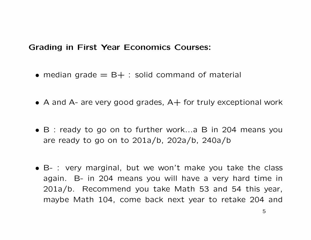
Grading in First Year Economics Courses:

• median grade = B+ : solid command of material

• A and A- are very good grades, A+ for truly exceptional work

• B : ready to go on to further work...a B in 204 means you

are ready to go on to 201a/b, 202a/b, 240a/b

• B- : very marginal, but we won’t make you take the class

again. B- in 204 means you will have a very hard time in

201a/b. Recommend you take Math 53 and 54 this year,

maybe Math 104, come back next year to retake 204 and

5

take 201a/b. B- is a passing grade, but you must maintain

a B average

• C: not passing. Definitely not ready for 201a/b, 202a/b,

240a/b. Take Math 53-54 this year, maybe Math 104, retake

204 next year

• 204 with at least a B- (or a waiver from 204 requirement) is

a strictly enforced prerequisite for enrollment in 201a/b

• F: means you didn’t take the final exam. Be sure to withdraw

if you don’t or can’t take the final.

Resources:

Book: de la Fuente, Mathematical Methods and Models for

Economists

Chris Shannon’s lecture notes: for every lecture + supplements

for several topics

Be sure to read Corrections Handout with dlF

Seek out other references

6

Goals for 204

• present some particular concepts and results used in first-yeareconomics courses 201a/b, 202a/b, 240a/b

• develop basic math skills and knowledge needed to work asa professional economist and read academic economics

• develop ability to read, evaluate and compose proofs...essentialfor reading and working in all branches of economics - theo-retical, empirical, experimental

• not to review Math 53 + 54. If you are weak on this material,take Math 53-54 this year, and take 204 next year.

7

Learning by Doing

• to learn this sort of mathematics you need to do more than

just read the book and notes and listen to lectures

• active reading: work through each line, be sure you know

how to get from one line to the next

• active listening: follow each step as we work through argu-

ments in class

• working problems: the most valuable part of the class

8

• you can work in groups but, always try to work through all

of the problems on your own before talking to others

• best test of understanding: can you explain it to others

Methods of Proof

• Deduction

• Contraposition

• Induction

• Contradiction

We’ll examine each of these in turn.

9

Proof by Deduction

Proof by Deduction: A list of statements, the last of which is

the statement to be proven. Each statement in the list is either

• an axiom: a fundamental assumption about mathematics, or

part of definition of the object under study; or

• a previously established theorem; or

• follows from previous statements in the list by a valid rule of

inference

10

Proof by Deduction

Example: Prove that the function f(x) = x2 is continuous at

x = 5.

Recall from one-variable calculus that f(x) = x2 is continuous

at x = 5 means

∀ε > 0 ∃δ > 0 s.t. |x− 5| < δ ⇒ |f(x)− f(5)| < ε

That is, “for every ε > 0 there exists a δ > 0 such that whenever

x is within δ of 5, f(x) is within ε of f(5).”

To prove the claim, we must systematically verify that this defi-

nition is satisfied.11

Proof. Let ε > 0 be given. Let

δ = min{

1,ε

11

}> 0

Where did that come from ? Suppose |x − 5| < δ. Since δ ≤ 1,4 < x < 6, so 9 < x+ 5 < 11 and |x+ 5| < 11. Then

|f(x)− f(5)| = |x2 − 25|= |(x+ 5)(x− 5)|= |x+ 5||x− 5|< 11 · δ≤ 11 ·

ε

11= ε

Thus, we have shown that for every ε > 0, there exists δ > 0such that |x − 5| < δ ⇒ |f(x) − f(5)| < ε, so f is continuous atx = 5.

Proof by Contraposition

Recall some basics of logic.

¬P means “P is false.”

P ∧Q means “P is true and Q is true.”

P ∨Q means “P is true or Q is true (or possibly both).”

¬P ∧Q means (¬P ) ∧Q; ¬P ∨Q means (¬P ) ∨Q.

P ⇒ Q means “whenever P is satisfied, Q is also satisfied.”

Formally, P ⇒ Q is equivalent to ¬P ∨Q.

12

Proof by Contraposition

The contrapositive of the statement P ⇒ Q is the statement

¬Q⇒ ¬P .

Theorem 1. P ⇒ Q is true if and only if ¬Q⇒ ¬P is true.

Proof. Suppose P ⇒ Q is true. Then either P is false, or Q is true

(or possibly both). Therefore, either ¬P is true, or ¬Q is false

(or possibly both), so ¬(¬Q) ∨ (¬P ) is true, that is, ¬Q⇒ ¬P is

true.

Conversely, suppose ¬Q ⇒ ¬P is true. Then either ¬Q is false,

or ¬P is true (or possibly both), so either Q is true, or P is false

(or possibly both), so ¬P ∨Q is true, so P ⇒ Q is true.

13

Proof by Induction

We illustrate with an example:

Theorem 2. For every n ∈ N0 = {0,1,2,3, . . .},n∑

k=1

k =n(n+ 1)

2

i.e. 1 + 2 + · · ·+ n = n(n+1)2 .

Proof. Base step n = 0: LHS =∑0k=1 k = the empty sum =

0. RHS = 0·12 = 0

So the claim is true for n = 0.

14

Induction step: Suppose

n∑k=1

k =n(n+ 1)

2for some n ≥ 0

We must show that

n+1∑k=1

k =(n+ 1)((n+ 1) + 1)

2

LHS =n+1∑k=1

k

=n∑

k=1

k + (n+ 1)

=n(n+ 1)

2+ (n+ 1) by the Induction hypothesis

= (n+ 1)(n

2+ 1

)=

(n+ 1)(n+ 2)

2

RHS =(n+ 1)((n+ 1) + 1)

2

=(n+ 1)(n+ 2)

2= LHS

So by mathematical induction,∑nk=1 k = n(n+1)

2 for all n ∈ N0.

Proof by Contradiction

Assume the negation of what is claimed, and work toward a

contradiction.

Theorem 3. There is no rational number q such that q2 = 2.

Proof. Suppose q2 = 2 where q ∈ Q. Then we can write q = mn

for some integers m,n ∈ Z. Moreover, we can assume that m

and n have no common factor; if they did, we could divide it

out.

2 = q2 =m2

n2

Therefore, m2 = 2n2, so m2 is even.

15

We claim that m is even. If not, then m is odd, so m = 2p + 1

for some p ∈ Z. Then

m2 = (2p+ 1)2

= 4p2 + 4p+ 1

= 2(2p2 + 2p) + 1

which is odd, contradiction. Therefore, m is even, so m = 2r for

some r ∈ Z.

4r2 = (2r)2

= m2

= 2n2

n2 = 2r2

So n2 is even, which implies (by the argument given above) that

n is even. Therefore, n = 2s for some s ∈ Z, so m and n have a

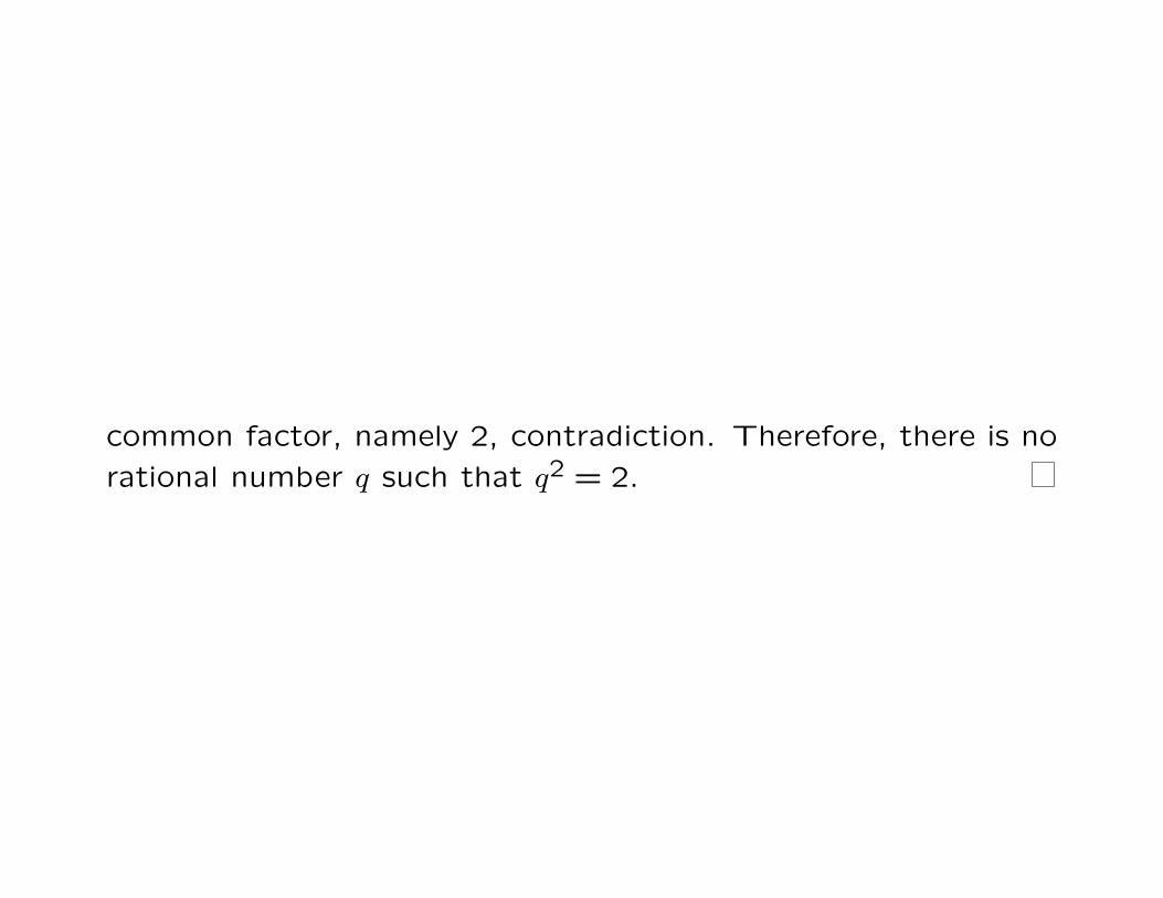
common factor, namely 2, contradiction. Therefore, there is no

rational number q such that q2 = 2.

Equivalence RelationsDefinition 1. A binary relation R from X to Y is a subset R ⊆X × Y . We write xRy if (x, y) ∈ R and “not xRy” if (x, y) 6∈ R.R ⊆ X ×X is a binary relation on X.

Example: Suppose f : X → Y is a function from X to Y . Thebinary relation R ⊆ X × Y defined by

xRy ⇐⇒ f(x) = y

is exactly the graph of the function f . A function can be consid-ered a binary relation R from X to Y such that for each x ∈ Xthere exists exactly one y ∈ Y such that (x, y) ∈ R.

Example: Suppose X = {1,2,3} and R is the binary relation onX given by R = {(1,1), (2,1), (2,2), (3,1), (3,2), (3,3)}. This isthe binary relation “is weakly greater than,” or ≥.

16

Equivalence Relations

Definition 2. A binary relation R on X is

(i) reflexive if ∀x ∈ X,xRx

(ii) symmetric if ∀x, y ∈ X,xRy ⇔ yRx

(iii) transitive if ∀x, y, z ∈ X, (xRy ∧ yRz)⇒ xRz

Definition 3. A binary relation R on X is an equivalence relation

if it is reflexive, symmetric and transitive.

17

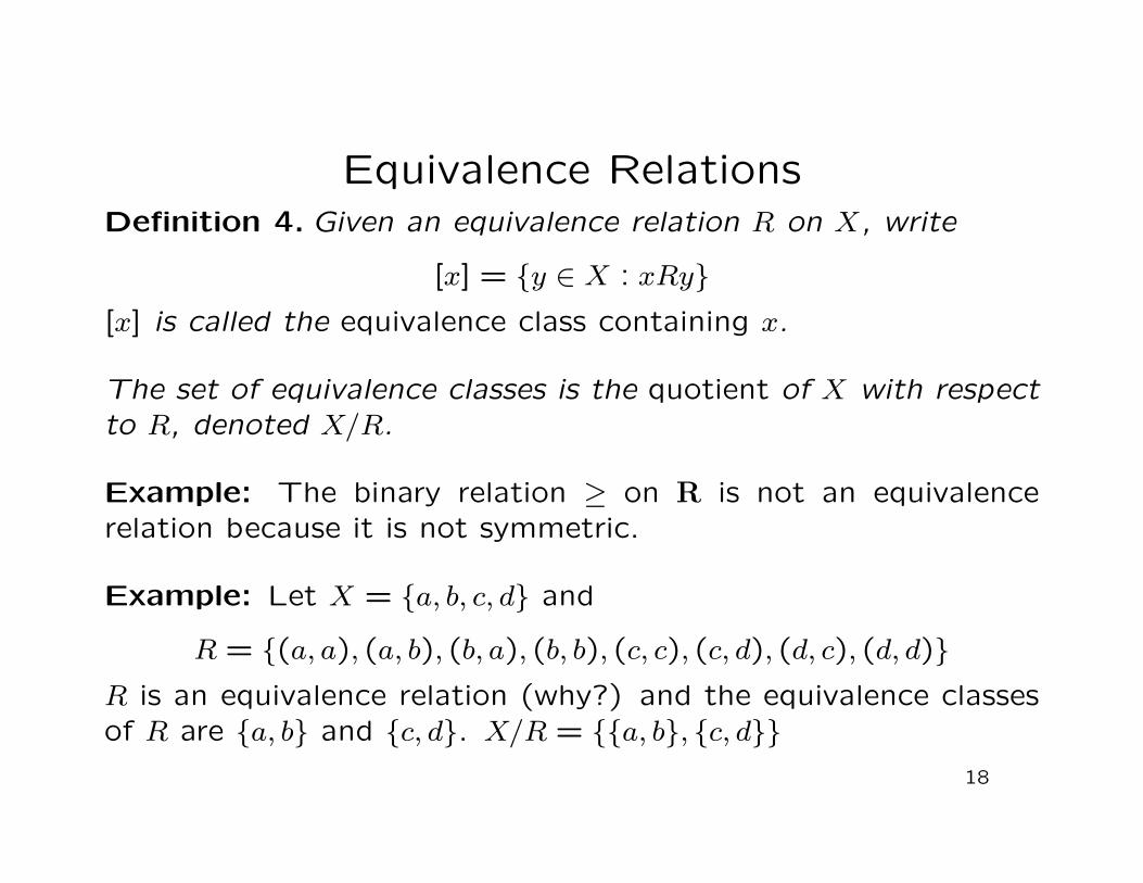
Equivalence RelationsDefinition 4. Given an equivalence relation R on X, write

[x] = {y ∈ X : xRy}[x] is called the equivalence class containing x.

The set of equivalence classes is the quotient of X with respectto R, denoted X/R.

Example: The binary relation ≥ on R is not an equivalencerelation because it is not symmetric.

Example: Let X = {a, b, c, d} and

R = {(a, a), (a, b), (b, a), (b, b), (c, c), (c, d), (d, c), (d, d)}R is an equivalence relation (why?) and the equivalence classesof R are {a, b} and {c, d}. X/R = {{a, b}, {c, d}}

18

Equivalence Relations

The equivalence classes of an equivalence relation form a parti-

tion of X: every element of X belongs to exactly one equivalence

class.

Theorem 4. Let R be an equivalence relation on X. Then ∀x ∈X,x ∈ [x]. Given x, y ∈ X, either [x] = [y] or [x] ∩ [y] = ∅.

Proof. If x ∈ X, then xRx because R is reflexive, so x ∈ [x].

Suppose x, y ∈ X. If [x] ∩ [y] = ∅, we’re done. So suppose

[x]∩ [y] 6= ∅. We must show that [x] = [y], i.e. that the elements

of [x] are exactly the same as the elements of [y].

19

Choose z ∈ [x] ∩ [y]. Then z ∈ [x], so xRz. By symmetry, zRx.

Also z ∈ [y], so yRz. By symmetry again, zRy. Now choose

w ∈ [x]. By definition, xRw. Since zRx and R is transitive, zRw.

By symmetry, wRz. Since zRy, wRy by transitivity again. By

symmetry, yRw, so w ∈ [y], which shows that [x] ⊆ [y].

Similarly, [y] ⊆ [x], so [x] = [y].

Cardinality

Definition 5. Two sets A,B are numerically equivalent ( or have

the same cardinality) if there is a bijection f : A→ B, that is, a

function f : A→ B that is 1-1 (a 6= a′ ⇒ f(a) 6= f(a′)), and onto

(∀b ∈ B ∃a ∈ A s.t. f(a) = b).

Example: A = {2,4,6, . . . ,50} is numerically equivalent to the

set {1,2, . . . ,25} under the function f(n) = 2n.

B = {1,4,9,16,25,36,49 . . .} = {n2 : n ∈ N} is numerically equiv-

alent to N.

20

Cardinality

A set is either finite or infinite. A set is finite if it is numerically

equivalent to {1, . . . , n} for some n. A set that is not finite is

infinite.

In particular, A = {2,4,6, . . . ,50} is finite, B = {1,4,9,16,25,36,49 . . .}is infinite.

A set is countable if it is numerically equivalent to the set of

natural numbers N = {1,2,3, . . .}. An infinite set that is not

countable is called uncountable.

21

Cardinality

Example: The set of integers Z is countable.

Z = {0,1,−1,2,−2, . . .}

Define f : N→ Z by

f(1) = 0

f(2) = 1

f(3) = −1...

f(n) = (−1)n⌊n

2

⌋where bxc is the greatest integer less than or equal to x. It is

straightforward to verify that f is one-to-one and onto.

22

Cardinality

Theorem 5. The set of rational numbers Q is countable.

“Picture Proof”:

Q ={m

n: m,n ∈ Z, n 6= 0

}=

{m

n: m ∈ Z, n ∈ N

}

23

m0 1 −1 2 −2

1 0 → 1 −1 → 2 −2↙ ↗ ↙ ↗

2 0 12 −1

2 1 −1↓ ↗ ↙ ↗

n 3 0 13 −1

323 −2

3↙ ↗

4 0 14 −1

412 −1

2↓ ↗

5 0 15 −1

525 −2

5

Go back and forth on upward-sloping diagonals, omitting the

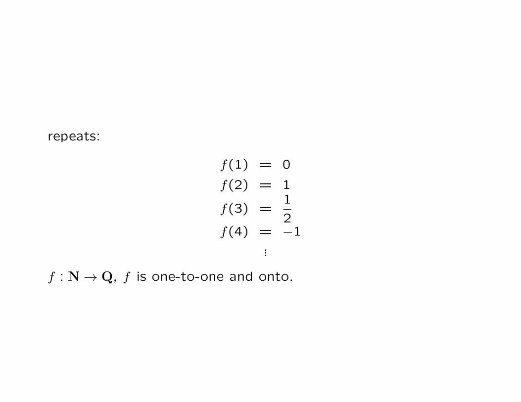
repeats:

f(1) = 0

f(2) = 1

f(3) =1

2f(4) = −1

...

f : N→ Q, f is one-to-one and onto.