ecology and conservation of breeding lapwings in upland grassland systems effects of agricultural...

ECOLOGY AND CONSERVATION OF

BREEDING LAPWINGS IN UPLAND

GRASSLAND SYSTEMS: EFFECTS OF AGRICULTURAL MANAGEMENT

AND SOIL PROPERTIES

Heather M. McCallum

September 2012

A thesis submitted for the degree of Doctor of Philosophy in the

School of Natural Sciences: Biological and Environmental Sciences

University of Stirling

i

Abstract

Agriculture is the principal land use throughout Europe and agricultural intensification has been

implicated in large reductions in biodiversity, with the negative effects on birds particularly well

documented. The lapwing (Vanellus vanellus) is one such species where changes in farming

practices has reduced the suitability and quality of breeding habitat, leading to a drop in

population size that has been so severe as to warrant its addition to the Red List of Birds of

Conservation Concern in the UK. Lowland areas, where agricultural intensification has generally

been most pronounced, have been worst affected, however, more recently declines in marginal

upland areas, previously considered refuges for breeding wader populations, have been

identified.

An upland livestock farm in Stirlingshire that uses an in-bye system of fodder crop management

and has unusually high densities of breeding lapwings provides a basis for this project to test

causal hypotheses for the decline of upland lapwing populations and to identify potential

conservation management solutions. Specifically this farm plants a forage brassica in an in-bye

field for two consecutive years, followed by reseeding with grass and seven, out of sixteen, in-bye

fields have undergone this regime at the study site since 1997. Fields that had undergone fodder

crop management supported almost 60% more lapwings than comparable fields that had not

previously been planted with the fodder crop. Lapwing density was highest in the year after the

fodder crop was planted, once it had been grazed, which results in a high percentage of bare

ground, likely to be attractive to nesting lapwings. Lapwing densities remained above that which

occurred in fields that had not undergone fodder crop management for a further four years after

the field had been returned to grass. The effect of management on lapwing food resources and

nesting structure was tested through a field experiment; liming increased the abundance of

Allolobophora chlorotica, an earthworm species that was associated with chick foraging location

ii

at the study site, suggesting that lapwings may benefit from liming conducted as part of fodder

crop management.

The relationship between lapwings and soil pH is further explored across 89 sites on mainland

Scotland, using soil property data to improve the predictive power of habitat association models,

something which has not previously been done for any farmland bird. Adding soil and

topographical data to habitat models, based on established relationships between breeding

lapwings and their habitat, improved model fit by almost 60%, indicating that soil properties

influence the distribution of this species. The density of breeding lapwings was highest at higher

altitude sites, but only when the soil was relatively less peaty and less acidic, providing further

support for the hypothesis that agricultural liming benefits lapwings.

In addition to assessing the conservation benefit of fodder crop management, the economic costs

are also considered. Fodder crop management provides a source of livestock fodder in the

autumn and winter during a period when forage demands outstrip grass growth, and ultimately

improves the grazing quality of the grass that is replaced; this system currently operates outside

of any agri-environment scheme (AES). However, at the study site, planting of the fodder crop

and grass is delayed to avoid agriculture operations during the breeding season, which reduces

yield and hence profitability. An initial estimate of £200 ha-1 is suggested as an incentive to

encourage wider adoption of fodder crop management in a “lapwing friendly” manner, although

further work is required to determine if this payment level is appropriate and the current method

of AES implementation may limit the suitability of fodder crop management as an AES.

The results indicate that agricultural liming could benefit breeding lapwings in pasture fields

where soil pH falls below pH 5.2, by increasing earthworm abundance. Where soil pH is below pH

5.2, liming should provide a cost effective mechanism for farmers to improve grass yields. Regular

soil testing and liming in response to low pH, within improved or semi-improved grassland fields,

iii

where management activities such as use of nitrogen fertiliser can contribute to soil acidification,

should be advocated to farmers in marginal areas as a mechanism for improving grass

productivity whilst potentially benefitting breeding lapwing and other species where earthworms

contribute significantly to their diet.

iv

Declaration

I declare that this thesis has been composed by myself and embodies the results of my own

research. Where work was carried out in collaboration with others, I have acknowledged the

nature and extent of their work.

…………………………………………………………………….

Heather M. McCallum

v

Acknowledgements

This research was funded by the University of Stirling and the Royal Society for the Protection of

Birds. I would like to thank my supervisors for their support, advice, encouragement, and above

all their genuine interest in the project for the past four years. I had a large supervisory team,

with three supervisors at the University: Kirsty Park, Dave Goulson and Nick Hanley, and four key

members of staff at RSPB who have been involved in a supervisory role for all or part of the

project: Jerry Wilson, Mark O’Brien, Rob Sheldon and Dave Beaumont. I am particularly grateful

to Kirsty and Jerry for the wealth of feedback they have provided on earlier drafts and for

statistical advice, to OB for teaching me how to find lapwing nests, providing me with his lapwing

data for chapter 4 and even responding to emails for help after relocating to Fiji, to Rob for

digging numerous soil cores at the field trial and making it look easy, and for being as good as he

claimed to be at finding lapwing chicks, and to Dave B for coming up with the project idea, the

funding and for talking me into doing a PhD in the first place!

This PhD could not have taken place without the support of Alistair Robb, the farmer at Townhead

Farm. I am extremely grateful to him for allowing me to spend so much time on his farm, helping

organise setting up the field experiment and sorting out extra lime when there was a mix up with

this in the final year, providing information on his management and for caring about the birds that

use his farm.

I would also like to thank Willie Owen, Muirpark Farm and Andrew Morton, Lochend Farm for

allowing me access to their farms to carry out wader surveys and collect soil cores. Thank you to

the staff and volunteers at RSPB’s Geltsdale reserve for putting in some trial management for me

and carrying out feeding observations. Additionally thanks to staff at the RSPB’s reserve on The

Oa, Islay for setting up additional trial management.

vi

For help with field work I am particularly grateful to Gail Robertson, who gave up so much of her

time voluntarily to assist during my 2nd field season - I’m so pleased that she is now doing her own

PhD! I would also like to thank Madeleine Murtagh for assistance during the 3rd field season and

both Laura Kubasiewicz and Elisa Fuentes-Montemayor for providing additional help. I would like

to thank the technical staff at Stirling University for their support, in particular Helen Ewing for

showing me how the soil lab operates, Willie Thomson for fixing the yagi-antennae and James

Weir for making the ground “bumpometer”.

I would not have been able to undertake the radio-tracking work without training in ringing and

attaching tags from Jen Smart (RSPB), with additional training in radio-tracking from Claire Smith

(RSPB) and training in ringing from Rob Campbell – thanks all. Thank you also to Malcolm Ausden

(RSPB) for training in earthworm identification. I would also like to thank John Vipond (SAC) for

discussing fodder crop management and Amy Corrigan (RSPB) for information on agricultural

policy.

Thank you to Alessandro Gimona and Laura Poggio of the James Hutton Institute for providing soil

property data for Chapter 4. In addition the data unit at RSPB extracted topographical data from

GIS which was used in this chapter.

I have made some fantastic friends during the course of my PhD and could not have got through

this without them. I’ve enjoyed numerous much needed coffee breaks with Lynne, Nicky, Dani

and Rachael, who have all been great office mates! Thanks as well to Kirsty’s research group for

interesting discussions on my and their research, in particular thanks to Jeroen Minderman for

knowing a lot about stats and R and being happy to answer lots of questions.

Thank you also to the support and encouragement from my family and for passing on the

determination genes necessary for getting me this far!

vii

Finally I could not have completed this PhD without Ewan’s support, his excel wizardry saved me

so much time and stress, he’s put up with me working very long hours particularly during field

work and write-up, been able to cope with the “emotional rollercoaster” of doing a PhD, calmed

me down on many occasions and even dug a few soil cores in the first year!

i

Contents Abstract ................................................................................................................................................ i

Declaration ......................................................................................................................................... iv

Acknowledgements ............................................................................................................................. v

Chapter 1 General introduction ......................................................................................................... 1

1.1 Agriculture and declines in biodiversity ................................................................................... 1

1.2 The lapwing .............................................................................................................................. 2

1.2.1 Declines and conservation status............................................................................... 2

1.2.2 Breeding ecology and negative effects of agricultural intensification ....................... 2

1.2.3 Food resources ........................................................................................................... 5

1.2.4 Agri-environment schemes ........................................................................................ 6

1.3 Linking soil pH, earthworms and lapwings ............................................................................... 7

1.4 The history of lime use in Great Britain ................................................................................... 9

1.5 Research objectives................................................................................................................ 15

Chapter 2 Lapwing habitat use at a high density site in upland Scotland ....................................... 17

2.1 Abstract ............................................................................................................................ 17

2.2 Introduction ..................................................................................................................... 18

2.3 Methods ........................................................................................................................... 21

2.3.1 Study site .................................................................................................................. 21

2.3.2 Comparisons between fields .................................................................................... 26

2.3.3 Comparisons within fields ........................................................................................ 28

2.3.4 Analysis ..................................................................................................................... 33

ii

2.4 Results .............................................................................................................................. 38



2.5 Discussion ......................................................................................................................... 51



Chapter 3 The effect of fodder crops and liming on factors important for breeding lapwings:

vegetation structure and food resources ........................................................................................ 59

3.1 Abstract ............................................................................................................................ 59

3.2 Introduction ..................................................................................................................... 60

3.3 Methods ........................................................................................................................... 62

3.3.1 Field experiment ...................................................................................................... 62

3.3.2 Between-field correlative study ............................................................................... 68

3.4 Results .............................................................................................................................. 72

3.4.1 Field experiment ...................................................................................................... 72

3.4.2 Between-field correlative study ............................................................................... 88

3.5 Discussion ......................................................................................................................... 96

3.6 Appendix A – Soil pH Correction Offset ......................................................................... 104

3.7 Appendix B – Trial management at RSPB Geltsdale ....................................................... 106

Chapter 4 Can soil properties improve habitat association models for breeding lapwings? ........ 109

4.1 Abstract ................................................................................................................................ 109

4.2 Introduction ......................................................................................................................... 109

iii

4.3 Methods ............................................................................................................................... 111

4.3.1 Analysis ................................................................................................................... 115

4.4 Results .................................................................................................................................. 122

4.5 Discussion ............................................................................................................................. 135

Chapter 5 The economic costs and benefits of managing upland grassland systems in a “lapwing

friendly” manner ............................................................................................................................ 141

5.1 Abstract ................................................................................................................................ 141

5.2 Introduction ......................................................................................................................... 142

5.3 Methods ............................................................................................................................... 144

5.3.1 Estimating profits from fodder crop management ................................................ 144

5.3.2 Estimating profits from alternative management systems ................................... 146

5.4 Results .................................................................................................................................. 147

5.4.1 The costs and benefits of fodder crop management ............................................. 147

5.4.2 Comparing the costs and benefits of fodder crop management with other

management systems ............................................................................................................ 149

5.5 Discussion ............................................................................................................................. 154

5.5.1 Sources of uncertainty in profit margins ................................................................ 154

5.5.2 The cost of agricultural inputs ............................................................................... 156

5.5.3 Potential loss of income due to delaying agricultural operations for lapwings ..... 158

5.6 Appendix A – Variation in lamb prices ................................................................................. 159

Chapter 6 General discussion......................................................................................................... 160

6.1 Key findings .......................................................................................................................... 160

iv

6.1.1 Ecology ................................................................................................................... 160

6.1.2 Economics .............................................................................................................. 164

6.2 Potential wider effects of management .............................................................................. 165

6.3 Policy implications ................................................................................................................ 167

6.3.1 Planting fodder crops ............................................................................................. 168

6.3.2 Lime use ................................................................................................................. 169

6.3.3 Potential limitations for implementation of fodder crop management as an AES 169

6.4 Further research ................................................................................................................... 170

References.................................................................................................................................. 172

1

Chapter 1 General introduction

1.1 Agriculture and declines in biodiversity

Agriculture is the principal land use throughout Europe and accounts for approximately 70% of

land in the UK (DEFRA 2012). The Common Agricultural Policy (CAP), which was introduced

shortly after World War II, has been instrumental in driving agricultural intensification by paying

farmers subsidies for production, leading to artificially high prices and vast quantities of surplus

food (Krebs et al. 1999). With its dominance in the landscape, agriculture is an important habitat

for many species and over half of all European biodiversity is dependent on farmland (Kleijn

2012). Agricultural intensification has been implicated in widespread d declines in biodiversity,

with negative effects of agricultural processes on birds particularly well documented (Krebs et al.

1999, Stoate et al. 2001, Robinson & Sutherland 2002, Newton 2004).

Intensification has resulted in simplification of the farmed landscape and a significant loss in

habitat heterogeneity (Chamberlain et al. 2000, Wilson, Evans & Grice 2009). Changes which have

contributed to this include increased field sizes, removal of hedgerows and field margins and a

decline in mixed farming systems, with livestock farming now occurring predominantly in the west

of the UK and arable mainly in the east. Faster growing varieties of crops and grass, along with

increased use of fertilisers, herbicides and pesticides have also contributed to large increases in

production, with the result that there is less space and reduced habitat quality for many species

(Vickery et al. 2001, Newton 2004). Further changes include large scale land drainage for

conversion to arable land or increased grass productivity, increased stocking densities facilitated

by increased grass production and a change from spring to autumn sowing of arable crops.

2

1.2 The lapwing

The Northern Lapwing (Vanellus vanellus, from now on referred to as lapwing) is “one of the

losers: everything that could go wrong has gone wrong: field drainage, over-grazing, silage

production, autumn sowing.….” (Marren 2002, p145).

1.2.1 Declines and conservation status

The global population of lapwings is estimated to be between 5 and 10 million individuals and this

very large population size coupled with the broad distribution of lapwings within the Palearctic,

mean that this species falls within the Least Concern category on the IUCN Red List, despite recent

declines in numbers (BirdLife International 2012a). Between 50% and 74% of the world’s

lapwings breed in Europe, and recent population declines here have led to lapwings being

considered of unfavourable conservation status in Europe (SPEC 2; Birdlife International 2004).

Within Europe, population declines have been particularly severe in Russia, the Netherlands and

the UK (Birdlife International 2004) and lapwings were added to the Red List of Birds of

Conservation Concern in the UK in 2009 (Eaton et al. 2009). Declines in breeding lapwings have

been linked to agricultural intensification and, in the UK, declines have been most severe in

lowland areas, where agricultural intensification has been most pronounced. Worryingly, recent

declines in marginal upland areas, previously considered refuges for breeding wader populations,

have been identified (Taylor & Grant 2004, Henderson et al. 2004).

1.2.2 Breeding ecology and negative effects of agricultural intensification

Like most other species of wader, lapwings nest on the ground (Mullarney et al. 1999), typically

laying a clutch of four eggs within a simple scrape (Klomp 1954). If the clutch is lost during the

incubation period then the female will often lay a replacement clutch, however, only one brood of

chicks will be raised in a breeding season and if the chicks are lost, any further attempt at

3

breeding that year is unlikely (Klomp 1951, Beintema & Muskens 1987, Parish, Thomson &

Coulson 1997).

Lapwings nest in both arable and pasture fields, though the choice of nest site is restricted to

areas with short vegetation or bare ground, which enables good visibility around the nest to see

approaching predators (Klomp 1954, Whittingham & Evans 2004, Shrubb 2007). Early detection

of predators is important as these will be mobbed, or chased off by lapwings to defend their nests

(Elliot 1985). Nest defence is communal and nest failure due to predation is higher in smaller

colonies (Berg, Lindberg & Kallebrink 1992). Nest sites with open views are selected often in

relatively flat, large fields, tending to avoid potential perches for avian predators and field

boundaries that restrict the visible area (Small 2002, Wallander, Isaksson & Lenberg 2006). In

addition to these anti-predation mechanisms, lapwings select nest sites which offer some degree

of camouflage to the eggs and the incubating bird such as, tussocky vegetation, areas of variable

sward height, areas with a mixture of vegetation and bare ground and damp areas with dull

green- brown sward (Galbraith 1989b, Baines 1990, Shrubb 2007).

In general, incubation starts once all four eggs have been laid, in order that they will hatch around

the same time. The incubation period is variable and was found to be anything between 21 and

28 days, with a mean of 25 days at a site in central Scotland (Galbraith 1988a). Lapwing chicks are

precocial and can feed themselves within a few hours of hatching (Cramp & Simmons 1983). The

adults’ role is threefold and involves leading them to suitable foraging areas, brooding them at

night and periodically during the day, until they are around two weeks old, and protecting them

against predators (Shrubb 2007). Whilst both arable and pasture fields are suitable for nesting,

chicks hatched in arable habitats will be led to more suitable foraging areas such as grazed

pasture, damp areas or grassy field margins (Galbraith 1988b, Sheldon et al. 2004). Chicks

hatched within pasture fields may stay within the vicinity of the nest area until fledging but

conversely they can also be moved over large distances (Cramp & Simmons 1983, Shrubb 2007).

4

Chicks fledge around 35 days after hatching and they are still dependent on their parents until

around 6 or 7 days after they can fly.

Within arable fields the change from spring to autumn sowing has reduced the availability of

preferred nesting habitat, with autumn sown crops too tall and dense by spring to be used

(Sheldon et al. 2004). The intensity of agricultural operations in spring has increased, leading to

high rates of nest destruction in fields that are otherwise suitable for nesting (Wilson, Evans &

Grice 2009). Faster growing varieties of crops and high fertiliser application rates mean that

spring sown crops quickly become too tall to be used, shortening the period that a field is suitable

for nesting and thus reducing the opportunity to replace clutches lost to agricultural operations.

Land drainage in grassland areas, which is often accompanied by increased fertiliser use and

reseeding with faster growing varieties, has led to taller more uniform swards, reducing the

suitability of pasture for nesting (Klomp 1954, Milsom et al. 2000, Vickery et al. 2001). Increased

grass production has facilitated increased stocking densities resulting in high rates of nest

destruction by trampling and high rates of nest abandonment by adults (Beintema & Muskens

1987, Pakanen, Luukkonen & Koivula 2011).

The suitability of arable fields for nesting depends on the proximity of chick rearing habitat such

as damp grassland and chicks that need to travel greater distances between the nest site and

brood rearing habitat are less likely to survive (Galbraith 1988). As such, large blocks of arable

land are rarely used by lapwings and the decline in mixed farming systems has led to a reduction

in the availability of arable nesting habitat that is close enough to chick rearing habitats to be

used or if it is used then chicks need to be moved over far larger distances reducing their chances

of survival (Stoate et al. 2001, Shrubb 2007, Wilson, Evans & Grice 2009).

5

1.2.3 Food resources

Lapwings are strongly associated with wet habitats and rely on wet features or moist soil to

supply their invertebrate prey (Berg 1993, McKeever 2003, Eglington et al. 2008, Eglington et al.

2010, Rhymer et al. 2010). Adults and chicks feed on a wide range of invertebrates including

beetles, flies, moths, ants, spiders, woodlice and earthworms (Cramp & Simmons 1983). Lapwings

are visual hunters that generally take their prey from the ground surface, and they have often

been observed foot trembling whilst hunting which is likely used to make hidden prey move or

bring earthworms up to the soil surface.

Whilst lapwings have an eclectic diet, a number of studies have identified earthworms as an

important prey resource, likely due to their relatively high calorific value coupled with their high

water content (Hogstedt 1974, Galbraith 1989a, Baines 1990, Beintema et al. 1991, Sheldon 2002,

Watkins 2007). Both adults and chicks take earthworms, although younger chicks may not be

capable of catching earthworms due to their small bill length. Beintema et al. (1991) suggested

that older chicks need to consume more earthworms in order to meet their increasing energy

demands as they approach fledging and they identified an increase in the number of earthworms

consumed with increasing chick age, despite decreasing availability of earthworms as the

breeding season progressed. Providing further support for Beintema et al.’s theory, Watkins

(2007) discovered that chicks older than 12 days foraged in relatively earthworm rich areas within

fields, whereas the opposite was true for younger chicks. Furthermore, positive relationships

have been identified between the number of earthworm chaetae within chick faecal samples,

chick age, growth rates and body condition, indicating an increase in earthworms consumed as

chicks age and increasing weight gain with increasing numbers of earthworms consumed (Sheldon

2002).

6

The pre-breeding / early breeding season is a particularly energetically demanding period for

adult lapwings (Galbraith 1989). Territorial males expend considerable energy on display flights,

reducing the amount of time available for foraging, whilst females put significant resources into

producing eggs. During this period, lapwings forage within fields that have relatively high prey

biomass (Galbraith 1989) and select earthworm rich patches within fields (Watkins 2007). Female

body condition is an important determinant of egg size, which in turn influences chick weight and

subsequently chick condition and survival, illustrating the importance of females consuming

adequate food resources prior to egg laying (Galbraith 1988a, Blomqvist, Johansson & Gotmark

1997). The length of the pre-laying period is highly negatively correlated with the abundance of

earthworms, indicating that lapwings can obtain adequate body condition for egg laying faster in

areas that are particularly earthworm rich (Hogstedt 1974).

Widespread land drainage is likely to have significantly reduced the abundance and availability of

invertebrate prey for lapwings (Baines 1990, Taylor & Grant 2004, Wilson, Evans & Grice 2009).

Higher yielding grass is also likely to have reduced the detectability of prey species within these

taller, more uniform swards (Devereux et al.2004).

1.2.4 Agri-environment schemes

Since 1992 the EU has provided funding through agri-environment schemes (AES) for famers to

adopt “environmentally friendly” farming practices (Stoate et al. 2001, Donald et al. 2006). To

date, the majority of AES targeted at breeding waders, including lapwings, have involved

compensatory payments for a reduction in land productivity brought about, for example, by

reducing livestock densities during the breeding season or raising the water table (Kleijn et al.

2001, Ausden & Hirons 2002, Kleijn & Zuijlen 2004, Ottvall & Smith 2006, Wilson, Vickery &

Pendlebury 2007, Verhulst, Kleijn & Berendse 2007, O’Brien & Wilson 2011). So far the success of

AES in increasing lapwing populations has been mixed.

7

Dutch AES, involving the restriction of agricultural operations on meadows during the wader

breeding season, stop nests from being destroyed by activities such as mowing. Reducing nest

destruction rates should have resulted in improved lapwing productivity in farms that are

managed under AES, however, breeding populations have not increased in comparison to those

on conventionally managed farms (Kleijn et al. 2001, Kleijn & Zuijlen 2004, Verhulst, Kleijn &

Berendse 2007). In the UK, populations of breeding waders on land managed under AES have

fared better than those on conventionally managed farms (Wilson et al. 2007, O’Brien and Wilson

2011). However the cost effectiveness of different options has been variable (Ausden & Hirons

2002, Wilson, Vickery & Pendlebury 2007), and the current area of land managed under AES is

estimated to fall well short of that required to reverse on-going population declines (O’Brien &

Wilson 2011).

1.3 Linking soil pH, earthworms and lapwings

One aspect of agriculture change which has not received much attention in relation to farmland

bird declines is soil pH. Soil pH is reduced by agricultural processes such as cropping and the use

of nitrogenous fertilisers, but also reduces naturally through leaching of calcium out of the soil

and has been reduced further in some areas by anthropogenic atmospheric acid deposition

(Rowell & Wild 1985, Gasser 1985, Johnston et al. 1986). Natural leaching of calcium out of the

soil is faster in areas with higher rainfall. Furthermore, the effect that both natural leaching and

acid deposition will have on soil pH is dependent on the buffering capacity of the underlying

geology, and in Scotland much of the underlying geology has poor buffering capacity against the

effects of acidification (Langan & Wilson 1992, Hornung et al. 1997).

The effects of soil acidification can be counteracted through agricultural liming which involves the

application of calcium oxide (quicklime), calcium carbonate (including limestone and chalk),

calcium hydroxide (slaked lime) or magnesium or dolomitic limestone, all known as lime, to the

8

land to raise soil pH (MAFF 1969, Goulding, McGrath & Johnston 1989). Failure to apply sufficient

lime to maintain soil pH at around pH 6 for grass and pH 6.5 for crops results in lower yields,

lower nutrient uptake by grass or crops, and inefficient use of nitrogenous fertilisers (Agricultural

Lime Association No Date).

The effect that agricultural liming has on soil pH means that it could affect the abundance of

earthworms, which have been identified as an important prey resource for breeding lapwings

(Section 1.3). Earthworms are sensitive to soil pH and very few earthworms occur in soils below

pH 4.3 (Edwards & Bohlen 1996). Earthworms can be broadly divided into three distinct

ecological groups; epigeic earthworms dwell at the surface, whilst endogeic species live in or just

below the root mat and anecic species form deep vertical burrows, and are capable of descending

at least one metre below the soil surface, coming up to the surface only periodically to obtain

food material such as dead leaves (Edwards & Bohlen 1996). Due to their distribution within the

soil, endogeic and epigeic species are available to foraging lapwings for more of the time than

anecic species, which are only available when they have come to the soil surface and are out of

reach when they are within their burrows. As lime is applied as a surface dressing, its effects on

soil pH is most pronounced in the top portion of the soil and it therefore seems likely that lime

has a greater effect on endogeic and epigeic than anecic earthworm species. Indeed reported

increases in earthworm abundance following liming are mainly for epigeic species (Deleport &

Tillier 1999, Bishop 2003, Potthof et al. 2008), although smaller increases in both endogeic and

anecic species were found by Potthof et al. (2008), and Bishop (2003) also identified an increase

in one endogeic species. Positive effects of liming on earthworms indicate that the practice of

agricultural liming may be of benefit to lapwings and in fact Brandsma (2004) identified an

increase in field use by both lapwings and black-tailed godwits (Limosa limosa) following increases

in earthworm abundance that occurred after liming.

9

1.4 The history of lime use in Great Britain

Lime has been used as a fertiliser in the UK for at least 2000 years (Gardner & Gardner 1957), but

with the advent of inorganic fertilisers in the 1850s, which provided far greater increases in yield

at lower cost, lime use began to decline (Johnston & Whinham 1980). In the 1930s, the UK

government, concerned by the prospect of war and declining soil fertility introduced a Lime

Subsidy for farmers (MAFF 1969). The quantity of agricultural lime purchased annually in the UK

increased from around half a million tonnes prior to the introduction of the subsidy to a peak of

around seven million tonnes in the late 1950s and early 1960s (Figure 1-1). The quantity of

agricultural lime sold annually started to drop again in 1965. Whilst The Ministry of Agriculture,

Forestry and Fisheries (MAFF) attributed this drop to the fact that large doses of lime applied in

the earlier part of the subsidy period had increased soil pH enough that only smaller doses of lime

were now required to maintain soil fertility, there was some evidence to suggest that the level of

liming occurring in the 1970s was not sufficient to maintain soil pH at optimum levels (The

Agricultural Lime Producers’ Council 1977, Church & Skinner 1986). The quantity of lime sold for

agricultural purposes in the UK continued to decline to just below two million tonnes in 1999 and

has remained around that level since. Current agricultural lime purchases are similar to that

which occurred at the start of the lime subsidy period in 1939 and are less than a third of that

purchased during the peak period.

10

Figure 1-1 The quantity of lime sold in Great Britain and Scotland for agricultural purposes, annually since 1938: data sources: Great Britain 1939 – 1976, The Lime Producers Council (1977), Great Britain 1980 – 1989, Wilkinson (1998), Great Britain 1990 – 2010, Hillier et al. (2003), Idoice, Bide & Brown (2012), Scotland 1939 – 1952, Gardener & Gardener 1957, Scotland 1998 – 2010, Scottish Government (2012).

The percentage of land limed in Great Britain rose slightly from the late 1960s until the mid-1970s

(Figure 1-2; Chalmers 2001). This increase occurred at a time when agricultural lime sales were

declining and this apparent disparity in the two measurements results from a decline in

application rates during this period (Chalmers, Kershaw & Leech 1990). The percentage of

agricultural land receiving lime inputs remained fairly steady from the mid-1970s until the end of

the 1980s, during a period of fluctuating lime sales. There was a peak in the percentage of land

that received lime in 1998 and since then the percentage of land limed annually has returned to

roughly the same as that which occurred in the 1980s, with around 6% of all agricultural land

limed annually corresponding with reasonably stable lime sales during this period. The

percentage of arable land limed annually was higher than the percentage of grassland limed

annually in all years, however, the difference has increased since 1969.

11

Figure 1-2 Percentage of agricultural land (arable and all grass) in Great Britain that received lime inputs from 1969 to present (no data found for 1989 – 1997). Data sources: 1969 – 1989, Chalmers, Kershaw & Leech (1990) and 1998 – 2011, DEFRA (1999 – 2012).

In England and Wales the percentage of arable land and the percentage of temporary grass (grass

that has been sown within the last five years) limed annually are fairly similar and have remained

at around 7% since 2000 (Figure 1-3a). The percentage of permanent grassland limed annually in

England and Wales is only around half as much as for temporary grassland. In Scotland there is a

much larger disparity in the percentages of arable land and grassland that are limed, with around

14% of all arable land limed annually since 1998, whereas only 4% of all grassland was limed

annually during the same period. As in England and Wales the percentage of temporary grassland

that is limed is higher than the percentage of permanent grassland. The percentage of arable

land limed annually in Scotland is almost twice as high as in England and Wales, whereas the

percentage of grassland limed is similar.

12

Figure 1-3 Percentage of arable and grassland (separated into grass under 5 years = temporary grass and grass > 5 years = permanent grass) limed between 1998 and 2011 in a) England and Wales, b) Scotland. Data source: DEFRA (1999 – 2012).

Differences in liming patterns between arable and grassland reflect higher soil pH requirements of

arable crops than grass (Agricultural Lime Association No date), but may also indicate under-

13

liming of grassland. Under-liming in arable areas can result in crop failure, whereas low grass

yields resulting from low soil pH may not be obvious, suggesting that there is a higher probability

of grassland being under-limed (Church & Skinner 1986). The Representative Soil Sampling

Scheme of England and Wales (RSSS) confirmed under-liming of grassland between 1978 and

1998, with a decline in soil pH in permanent grass detected, contrasting with an increase in soil pH

on arable land (Skinner, Church & Kershaw 1992, Skinner & Todd 1998, Webb et al. 2001). Spatial

analysis of the RSSS data reveals strong regional trends in pH with low soil pH and declines in pH

in Wales, the West Country and Northern England, areas that are dominated by livestock farms

(Figure 1-4; Baxter et al. 2006). A higher percentage of arable land is limed annually in Scotland in

comparison to England and Wales (Figure 1-3), implying that Scottish soils have higher lime

requirements and this is indeed the case with soil pH on average lower in Scotland, than in

England (Figure 1-5; Emmett et al. 2010).

Figure 1-4 Change in soil pH between 1971 and 2001 detected by the Representative Soil Sampling Scheme of England and Wales (RSSS), with declines in pH over this period indicated by blue colouration. Figure from Baxter et al. (2006).

14

Figure 1-5 Soil pH results in the UK, as found by the 2007 countryside survey, figure from Emmett et al. (2010).

In contrast to the results of the RSSS the Countryside Survey identified an increase in soil pH in

grassland areas as well as in arable areas between 1978 and 2007 and this was attributed to a

decrease in acid deposition during this period (Emmett et al. 2010). Increases in soil pH were

higher in England than in Scotland and in Scotland soil pH increases were generally confined to

the period between 1978 and 1998, with no further significant increases detected between 1998

and 2007.

In conclusion there has been a decline in lime use in Great Britain since a peak period in the

1960s. Arable land is much more likely to be limed than grassland, in particular permanent

grassland, and the RSSS indicates that permanent grassland has been under-limed, which may

have had negative consequences for earthworm abundance. However, a decline in acid

15

precipitation means that there has been an overall increase in soil pH (across all land uses)

between 1978 and 2007, although this survey did not look specifically at agricultural permanent

grasslands. Furthermore, changes in soil pH (and lime use) have not been examined in relation to

altitude and it is likely that soil acidification will be faster in upland areas due to higher leaching

rates associated with higher rainfall.

1.5 Research objectives

In contrast to the many negative effects that agriculture is known to have on breeding lapwings,

the principal objective of this thesis is to identify the driver(s) of the unusually high lapwing

densities, which occur at an upland livestock farm near to Stirling (Townhead Farm), that appear

to be linked to an in-bye management system employed here. The management system at the

study site involves planting a forage brassica (tyfon Brassica campestris x B.rapa) for two

consecutive years, in a field that was previously permanent pasture, prior to reseeding the field

with grass. This process ultimately improves grass productivity (EBLEX 2008), as well as providing

fodder for fattening of lambs over the winter (Koch et al. 1987). The ground is limed for up to

three years in the lead up to reseeding in order that the optimum soil pH for grass growth is

obtained. This process has been implemented on seven in-bye fields at the study site since 1997

and will be referred to as fodder crop management throughout this thesis.

There are a number of mechanisms by which the farm management may be benefitting breeding

lapwings, these are:-

1. Tyfon is grazed over the autumn / winter creating an open vegetation structure in the

spring, with a high percentage of bare ground, which is likely to be “attractive” to nesting

lapwings

16

2. Liming potentially increases earthworm abundance and as such food resources for

lapwings

3. There are many naturally wet areas on the farm which have not been drained and these

are likely to be important particularly during the chick rearing period

4. Both fox and crow control are carried out at the farm and in the surrounding area.

This thesis will specifically address the following questions:-

Are lapwing densities at the study site related to fodder crop management and what habitat

features are important for the lapwing population? (Chapter 2)

How does fodder crop management affect factors important for breeding lapwings: vegetation

structure and food resources? (Chapter 3)

Can soil properties improve habitat models for breeding lapwings? (Chapter 4)

Is fodder crop management economically viable and how does it compare to other in-bye

management strategies? (Chapter 5)

Finding out what is driving the unusually high densities of breeding lapwings at Townhead Farm

could have conservation benefits for a species that has undergone severe declines, by informing

future conservation management practices. Exploring the relationship between breeding

lapwings and soil properties may suggest areas where management should be targeted and

provide new ideas for conservation management to benefit breeding lapwings and potentially

other species. Furthermore, assessing the economic viability of the management system at

Townhead, will inform whether management recommendations from this thesis are likely to

require agri-environment funding or if they can be promoted without the need for a financial

incentive.

17

Chapter 2 Lapwing habitat use at a high density site in upland Scotland 2.1 Abstract

The lapwing has suffered significant declines in breeding populations across much of its range in

Europe. Declines have been linked to several aspects of agricultural intensification including land

drainage, increased fertiliser use and increased stocking densities. In contrast to the many

negative effects that increasing agricultural productivity has had on breeding lapwing populations,

this study explores the relationship between an economically viable farm management system

and breeding lapwings at a high density site in upland Scotland. Management involved planting of

a fodder crop for two consecutive years followed by reseeding with grass, with seven in-bye fields

at the farm undergoing this management since 1997. Breeding density was significantly higher in

fields that had undergone fodder crop management than those that had not, whilst controlling for

other field habitat parameters of importance to breeding lapwings. Density of breeding lapwings

was highest in the first year after the fodder crop was planted, but remained elevated above

levels in fields that had not undergone fodder crop management for approximately four years

after reseeding with grass. Sparse rush patches, which were more prevalent in grass fields that

had undergone fodder crop management, likely as a result of the management process, appeared

to be used preferentially for both nesting and chick rearing. Lapwing chick foraging location was

associated with high soil moisture and relatively high abundance of Allolobophora chlorotica, an

acid intolerant earthworm that may have benefitted from liming carried out as part of fodder crop

management. Implementing fodder crop management at other sites may have conservation

benefits for a species that has undergone severe declines; however, management must be

targeted at sites that have adequate densities of wet features if it is to be successful.

18

2.2 Introduction

Agriculture is the predominant land use across much of Europe and agricultural intensification has

resulted in widespread declines in many species that use farmland (Krebs et al. 1999, Stoate et al.

2001, Robinson & Sutherland 2002). Declines in farmland birds have been particularly well

documented (Chamberlain et al. 2000, Newton 2004). Agricultural land is the primary habitat

used by breeding lapwings (Vanellus vanellus; Shrubb 2007) and the severity of population

declines in this species led to its addition to the Red List of Birds of Conservation Concern in 2009

(Eaton et al. 2009). The lapwing is also a UK Biodiversity Action Plan priority species

(http://jncc.defra.gov.uk/page-5163, accessed 17 November 2011).

Declines in breeding lapwing abundance have been related to agricultural intensification, which

has brought about many changes in land management practices that have had negative effects on

the suitability of farmland as breeding habitat for lapwings (Hudson et al. 1994, Sheldon et al.

2004, Wilson, Evans & Grice 2009). Drainage of land to improve its agricultural productivity has

been particularly detrimental for lapwings (Taylor & Grant 2004), which like other wading birds

are reliant on wet habitats (Berg 1993, Eglington et al. 2008, Rhymer et al. 2010). Drying out of

soils leads to a reduction in the abundance and availability of soil and surface invertebrates

including earthworms (Edwards & Bohlen 1996, McKeever 2003), which have been identified as a

particularly important prey item (Galbraith 1989a, Beintema et al. 1991, Sheldon 2002).

The combination of land drainage and increased use of inorganic fertilisers on grasslands has

resulted in taller, denser and more uniform swards which are harder for lapwings to detect their

prey in (Vickery et al. 2001, Devereux et al. 2004). Since lapwings select nest sites with short

sward or bare ground, taller swards also reduce nest site availability (Klomp 1954, Milsom et al.

2000, O’Brien 2001, Shrubb 2007). Increased grass production means that pastures can support

greater stocking density and this can result in high rates of nest destruction by trampling or

http://jncc.defra.gov.uk/page-5163

19

increased likelihood of nest abandonment by incubating adults (Beintema & Muskens 1987,

Pakanen, Luukkonen & Koivula 2011).

Another feature of agricultural intensification has been the loss of mixed farming systems with

the majority of arable land now occurring in the south and east of the UK and grassland farms

more prevalent in the west (Newton 2004, Wilson, Evans & Grice 2009). Mixed farming systems

are particularly beneficial for lapwings as arable land, especially spring tillage, is a preferred

nesting habitat (Sheldon et al. 2004, Shrubb 2007) and in mixed farms this occurs in close

proximity to suitable chick rearing habitat, in the form of pasture (Galbraith 1988, Galbraith

1989b).

Since 1992 the EU has provided funding through agri-environment schemes (AES) for farmers to

adopt more “environmentally friendly” management practices. To date, AES in the UK for

breeding waders have focussed on compensatory payments for a reduction in land productivity

brought about, for example, by reducing livestock densities during the breeding season or raising

the water table (Ausden & Hirons 2002, Wilson, Vickery & Pendlebury 2007, O’Brien &Wilson

2011). So far AES for breeding waders have had limited success and have not been sufficient to

halt population declines in lapwings or other breeding wader species (Ausden & Hirons 2002,

Kleijn & Van Zuijlen 2004, Verhulst, Kleijn & Berendse 2007, O’Brien & Wilson 2011).

In contrast to the well documented negative effects of agricultural intensification on breeding

lapwings, an upland livestock farm in Stirlingshire, Scotland has unusually high densities of

breeding lapwings which appear to be linked to an economically viable management system at

the farm, which operates outside of any AES. This system involves planting of a forage brassica

(tyfon, Brassica campestris x B.rapa) for two consecutive years, prior to reseeding with grass;

from now on this process will be referred to as fodder crop management. Fodder crop

management ultimately improves grass productivity and fields are selected based on the

20

agricultural quality of the grassland, with fields with swards containing a relatively low percentage

of perennial rye-grass (Lolium perenne) and thus lower agriculturally productive grassland, chosen

by the farmer.

Management may be influencing the lapwing population at the site by grazing of tyfon creating an

“attractive” vegetation structure for nesting lapwing in the spring, with a high percentage of bare

ground. Liming which is carried out as part of the fodder crop management process may have

increased earthworm abundance through raising soil pH. Finally naturally wet areas that have not

been drained and are left unmanaged are likely to provide important habitat for lapwings

particularly during the chick rearing stage.

This study tests the hypothesis that high densities of lapwings at this farm are related to the

fodder crop management process, specifically addressing the following questions:-

Comparisons between fields

1. Is the density of breeding lapwings related to land management history, specifically in

regards to fodder crop management?

Comparisons within fields

2. Are lapwing nests associated with habitat patches within fields, such as wet unmanaged

patches?

3. Is lapwing chick foraging location associated with within field habitat characteristics such

as earthworm density that may relate to field management history?

21

2.3 Methods

2.3.1 Study site

This study took place at Townhead Farm, Stirlingshire, Scotland, which is a 315 ha upland (140 –

320 m altitude) livestock farm supporting approximately 1200 black-faced sheep and 50 limousin

cross cattle (Figure 2-1). The study site is part of the Clyde plateau volcanic formation, with

underlying geology of basalt and spilite laid down during the Carboniferous period (Geology

Roam, available from EDINA Digimap Ordnance Survey Service,

http://digimap.edina.ac.uk/geologyroam/mapper, accessed 7 April 2013). The soil derives from

basaltic rocks and mainly constitutes brown forest soils

(http://sifss.hutton.ac.uk/SSKIB_Stats.php, accessed 7 April 2013).

Figure 2-1 a) The location of the study site (Townhead Farm) in Scotland b) Ordnance Survey map of the study site showing topography of the site.

The farm comprises 120 ha of in-bye land (140 – 270 m altitude) and 195 ha of out-bye (175 – 320

m altitude, Figure 2-2, Figure 2-3). With in-bye defined as the enclosed fields used for either

arable or grass production, close into the farm house, which occur below the moorland wall,

whereas the out-bye is outside the moorland wall and is used for rough grazing only

(http://www.scotland.gov.uk/Topics/farmingrural/SRDP/RuralPriorities/Options/BrackenManage

a) b)

http://digimap.edina.ac.uk/geologyroam/mapper

http://sifss.hutton.ac.uk/SSKIB_Stats.php

http://www.scotland.gov.uk/Topics/farmingrural/SRDP/RuralPriorities/Options/BrackenManagement/DefinitionsofLandTypes

22

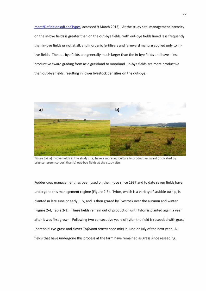
ment/DefinitionsofLandTypes, accessed 9 March 2013). At the study site, management intensity

on the in-bye fields is greater than on the out-bye fields, with out-bye fields limed less frequently

than in-bye fields or not at all, and inorganic fertilisers and farmyard manure applied only to in-

bye fields. The out-bye fields are generally much larger than the in-bye fields and have a less

productive sward grading from acid grassland to moorland. In-bye fields are more productive

than out-bye fields, resulting in lower livestock densities on the out-bye.

Figure 2-2 a) In-bye fields at the study site, have a more agriculturally productive sward (indicated by brighter green colour) than b) out-bye fields at the study site.

Fodder crop management has been used on the in-bye since 1997 and to date seven fields have

undergone this management regime (Figure 2-3). Tyfon, which is a variety of stubble turnip, is

planted in late June or early July, and is then grazed by livestock over the autumn and winter

(Figure 2-4, Table 2-1). These fields remain out of production until tyfon is planted again a year

after it was first grown. Following two consecutive years of tyfon the field is reseeded with grass

(perennial rye-grass and clover Trifolium repens seed mix) in June or July of the next year. All

fields that have undergone this process at the farm have remained as grass since reseeding.

a) b)

http://www.scotland.gov.uk/Topics/farmingrural/SRDP/RuralPriorities/Options/BrackenManagement/DefinitionsofLandTypes

23

Figure 2-3 Google Earth image of the study site. The out-bye is outlined in blue with the in-bye outlined in red. Fields that have undergone fodder crop management are outlined in black, with the years in which the fodder crop was planted shown for these fields. This image is from 2004 and the brown field indicates that this field had been tilled ready for grass reseeding but that the field that was planted with tyfon in 2004 had not yet been tilled.

Figure 2-4 a) Sheep grazing tyfon crop in autumn. b) In the spring following autumn / winter grazing, tyfon field has a high percentage of bare ground, with a lapwing nest on the grazed field.

a) b)

24 Table 2-1 Timings of fodder crop management process in comparison to lapwing use at the study site.

Farm management Late June / July Autumn / winter March

Year 1

Tyfon planted

Tyfon grazed

Most of crop has been grazed

Year 2

Tyfon planted

Tyfon grazed

Most of crop has been grazed

Year 3 Grass planted Grazing excluded for grass growth Grass grazed

Lapwing activity Leave for wintering grounds At wintering grounds Arrival for breeding

25

Fields selected for fodder crop management are on average further from the farmhouse than

those that have not been, indicating that proximity to the farmhouse did not influence selection

(Table 2-2). Whilst fields that were selected formerly for fodder crop management were of a

similar size to the majority of in-bye fields, the latter two fields that were chosen are relatively

small and these were likely selected to reduce the cost of management. Fields selected for fodder

crop management have a relatively low density of wet features suggesting that fields with high

densities of streams and ditches were avoided due to increased difficulty in manoeuvring the

machinery used to carry out fodder crop management.

Table 2-2 Characteristics of in-bye fields that have undergone fodder crop management at the study site compared to in-bye fields that have not. Data presented are means ± standard error.

Undergone fodder crop management

Not undergone fodder crop management

Distance from farm house (m) 334 ± 81 513 ± 150

Field Area (ha)

6.64 ± 1.08 8.65 ± 0.58

Altitude (m)

202 ± 9 201 ± 12

Slope

5.6 ± 0.4 5.0 ± 0.3

Density of streams and ditches (length/area)

60 ± 16 86 ± 28

Extent of field enclosure 0.17 ± 0.03 0.10 ± 0.03

Prior to growing tyfon, soil pH is tested. Lime (5 tonnes ha-1 annum-1) is applied in up to three

consecutive years with the first application at the time that tyfon is first planted. The objective of

liming is to raise soil pH to 5.8 to coincide with grass reseeding. Fertiliser (NPK, 2:1:1, 250 kg ha-1)

is applied at the same time as tyfon or grass is planted. Some fields have also had super triple

phosphate applied. In-bye fields that have not undergone fodder crop management have not

been reseeded since at least 1997. Reseeded grass fields (i.e. those that have undergone fodder

crop management) receive inorganic fertiliser (NPK, 2:1:1, 250 kg ha-1) annually, whereas non

reseeded in-bye fields receive this fertiliser less frequently. In-bye fields that have not undergone

fodder crop management are limed a maximum of once every five years.

26

Lapwings arrive at the farm from the beginning of March and leave at the end of the breeding

season, around the end of June / early July. The timing of operations at the farm is such that

planting of tyfon or grass occurs either at the end or after the breeding season so lapwing use will

only be affected in the year after management has occurred (Table 2-1).

2.3.2 Comparisons between fields

Lapwing density and field management history

Lapwing surveys

Lapwing surveys were carried out with varying numbers of repeated visits and by a number of

different observers in 2003 and from 2006 to 2011 (Table 2-3). Surveys followed the O’Brien and

Smith (1992) method, and were carried out on a field-by-field basis. Survey visits were conducted

on foot, walking to within 100 m of all points of each field and scanning ahead (up to 400 m) with

binoculars from appropriate vantage points. The position and behaviour of all lapwings were

marked on a 1:10000 Ordnance Survey map using standard British Trust of Ornithology (BTO)

codes. Lapwings were assigned to the first field in which they were noted, or if in display flight,

the field at the centre of their display.

Table 2-3 Wader survey visits carried out at the study site, initials denote surveyor: HMcC = Heather McCallum, M'OB = Mark O’Brien, DB = David Beaumont, JW= Jeremy Wilson, SD = Sarah Davis, DBr = Daniel Brown, AF = Adam Fraser, LB = Laura Black. Date for visits 2-4 followed O’Brien & Smith (1992), dates for visits 1 and 5 followed Bolton et al. (2011).

Visit 1 Visit 2 Visit 3 Visit 4 Visit 5

15 Mar - 17 Apr 18 - 30 Apr 1 - 21 May 22 May - 18 Jun 19 Jun - 8 Jul

2011

HMcC HMcC HMcC HMcC HMcC

2010

HMcC HMcC HMcC, DBr, AF HMcC HMcC

2009

HMcC HMcC HMcC HMcC HMcC

2008

HMcC, MO'B HMcC, DB, SD HMcC, MO'B, DB 2007

MO'B, DB

2006

MO'B, DB, JW 2003 LB LB LB

27

Visits 1 -4 were conducted within 1-4 hours of dawn or dusk and visit 5 took place between 0700

and 1330. Consecutive visits were at least 18 days apart. In 2003, 2006, 2007 and 2008, survey

visits were carried out in one morning or one evening. Between 2009 and 2011, it was necessary

to split each survey visit into two sessions, surveying approximately half of the farm in each

session. When possible split visits were done on consecutive days, however weather conditions

did not always allow this (surveys not carried out in continuous or heavy rain, low visibility or

when wind speeds were above Beaufort Force 4). All split visits were conducted within the space

of a week. Annual totals of lapwing pairs were calculated on a field by field basis by halving the

number of individuals (excluding flocks not exhibiting breeding behaviour) recorded on visit 2 or

3, selecting the visit where the maximum number of lapwings was recorded across the whole

farm (Barrett & Barrett 1984).

Measurement of field characteristics that influence the suitability of a field for breeding

lapwings

Data on field characteristics likely to influence the suitability of a field for breeding lapwings were

measured using ArcGIS 9.2 (ESRI inc 2006). The length of streams and ditches and field

boundaries were obtained from the OS Mastermap Topography Layer (EDINA Digimap Ordnance

Survey Service). This data was used to calculate the density of streams and ditches per hectare by

dividing the total length of these within each field by field area, giving an indication of field

wetness. Field slope was extracted from the OS digital terrain map (EDINA Digimap Ordnance

Survey Service). The proportion of the field perimeter with enclosed boundaries (either trees or

buildings) was calculated by measuring the length of perimeter made up of trees or buildings and

dividing this by total field perimeter.

28

2.3.3 Comparisons within fields

Defining habitat patch types within fields

To assess lapwing habitat use within fields, defined habitat patches within in-bye pasture fields

were mapped using a GPS (Garmin Etrex Vista HCx) in 2010.

Two types of habitat patch were identified and plotted onto a GIS:

Naturally wet areas, characterised by a high percentage of jointed rush (Juncus

articulatus), which were left uncultivated and un-drained by the farmer, from now on

referred to as unmanaged wet patches (Figure 2-5a & b)

Distinct patches of sparse rush (mainly soft rush J. effusus but in some patches also

jointed rush) with rush accounting for approximately 5% of the sward within a sparse rush

patch (Figure 2-5c & d)

Areas outside of these two habitat patches were mainly grass (Figure 2-5a, b & c).

29

Figure 2-5 Habitat types on the in-bye at the study site: a) unmanaged wet patch, outside of patch is mainly grass b) lapwing between two unmanaged wet patches on mainly grass area c) sparse rush patches within mainly grass d) close up of a sparse rush patch.

Nesting habitat use

Locating nests

Nests were located by looking for incubating adult lapwings with binoculars or a spotting scope in

2009, 2010 and 2011. Detailed descriptions of nest locations were made in order to find the nests

on the ground and confirm that they were still active on subsequent visits. Nest location was

marked using a GPS on the first visit to the nest and locations were transferred to the habitat GIS.

The habitat category for each nest location was extracted from the GIS after first converting the

habitat data to raster format (cell size 0.4 m x 0.4 m). Habitat type of each nest was defined as

the habitat that wholly contained the nest.

a)

b)

c)

d)

30

Chick foraging location

Radio-tagging chicks to estimate chick foraging location

A total of 19 lapwing chicks (10 in 2010, 9 in 2011) from separate broods were fitted with

Pip3Ag376 backpack mounted radio-tags (Biotrack Ltd, Dorset, UK). All chicks within a brood

were ringed using BTO metal rings. Coloured insulating tape was used on the ring to provide each

brood with a temporary unique colour marker. Radio-tagged chicks were re-caught at

approximately weekly intervals in order that tags that were beginning to come loose could be re-

glued.

Chick locations were estimated using triangulation by taking the bearing of the strongest signal

from the chick’s radio-tag (using a Sika receiver and three-element flexible Yagi antennae –

Biotrack Ltd, Dorset, UK) from a minimum of three locations in succession (White & Garrot 1990,

Kenward 2001). Estimated chick locations and the associated error ellipses (50% confidence)

were calculated using Lenth’s maximum likelihood estimator (White & Garrot 1990), using

Location of a Signal 4.0.3.7 (Ecological Software Solutions LLC 2010). Error ellipses incorporated

antennae error, which was established from a number of test triangulations carried out at the

study site (standard deviation 11.5). Chicks were located with triangulation around every one to

three days.

This work was carried out under SNH (9797) and BTO licences (C/5642).

Direct observations of chicks

In addition to triangulated locations, some radio-tagged chicks were sighted using direction of the

strongest signal to guide where to look for the chick. Fields were also searched visually (with a

spotting scope) for non radio-tagged chicks, using clues from adult behaviour to concentrate on

31

areas in which chicks were likely to be located. Visual searches for chicks were carried out no

more than once per day for each field. It was difficult to see chicks in unmanaged wet patches

due to taller vegetation in these areas; however, it was sometimes possible to ascertain that

chicks were using this habitat based purely on adult behaviour.

For all directly observed chicks, chick habitat use was assigned to the first habitat type that the

chick was observed in on that day. GPS locations were only obtained for directly observed chicks

if earthworm sampling was carried out for that observation (see below).

Earthworm sampling

To avoid repeated disturbance of chicks, earthworm sampling was conducted at a maximum

frequency of once per week per field for one chick location. Chick locations were either

estimated from triangulation and located using GPS, or directly observed, in which case a

waymark (GPS) was made at the time of earthworm collection (Table 2-4). At each chick location

four soil cores (10cm depth, 10.5cm diameter) were collected and these were paired with four

random soil cores which were taken from four separate random locations within the same field as

the chick was located. Random points were generated using the Sampling Tool extension (Finnen

& Menza 2007) within ArcGIS and were located in the field using GPS. For each soil core two soil

moisture measurements were taken within 15cm of the soil core location using a soil moisture

metre (HH2 moisture metre, SM200 moisture sensor, Delta-T Devices, Cambridge, England).

32

Table 2-4 Number of chick locations where earthworms were sampled within each field type, showing method used to locate chick.

In-bye

With history of fodder crop management

With no history of fodder crop management Out-bye Total

Estimated from triangulation 8 10 4 22

Direct observation of tagged chick 5 1 3 9

Direct observation of unmarked chick 3 4 1 8

Total 16 15 8 39

Soil cores were hand sorted in the laboratory to determine soil invertebrate abundance (Edwards

& Bohlen 1996). To avoid double counting of broken earthworms only earthworms with heads

were counted. Earthworms were identified to species level (Sims & Gerard 1985), with the

exception of juvenile earthworms of Lumbricus species or Aporrectodea caliginosa / Aporrectodea

rosea, which were assigned to one of these two groups based on colour, prostomium shape and

spacing of chaetae.

Assessing chick habitat use at foraging locations

To complement the earthworm data, habitat was assessed within the GIS for all chick and random

locations that earthworms were collected from. The mean error ellipse area for triangulated

locations was 4764 ± 1067 m2 which exceeded the mean area of unmanaged wet patches and

sparse rush patches (3155 ± 516 m2), thus making a high rate of habitat mis-classification likely if

habitat type was simply assigned to triangulated locations (Rettie & McLoughlin 1999). Instead

my approach here, to estimate chick habitat selection, was to compare the distance of chick

locations to the scarcer habitat patch types (unmanaged wet patches, sparse rush patches and

stream/ditches) with the distance of the paired random locations to these patches. Distances to

habitat features were measured using the Spatial Analyst tool.

33

2.3.4 Analysis

All statistical analyses were performed with R version 2.12.1 (R Development Core Team 2010).

GLMMs where the response variable was a count were implemented with Poisson errors and log

link, using the lme4 package (Bates & Maechler 2010). Loge field area was used as an offset in all

of the Poisson models and these models were checked for overdispersion by comparing the

residual deviance with the residual degrees of freedom. Pseudo r2 (from now on referred to as r2)

was calculated by correlating the predicted values with the observed data and squaring this (Zuur

et al. 2009).

Binomial GLMMs were conducted with the MASS package (Venables & Ripley 2002), using logit

link. Model fit was assessed by comparing the predicted probabilities calculated from the model

with the observed data within a confusion matrix, using the mean of the fitted values as the

threshold level above which a location was assigned as a chick rather than random location

(Fielding & Bell 1997).

Minimum adequate models were obtained using stepwise backwards selection, retaining all

explanatory variables that were significant at the 5% level.

Comparisons between fields

Three generalised linear mixed effects models (GLMMs) were implemented to test the

relationship between lapwing field use and field management history:

1. Do fields with a prior history of fodder crop management have higher lapwing densities?

If a field had been planted with tyfon, it was included in the “fodder crop” treatment group for all

lapwing surveys after this occurred. As tyfon was only grown in in-bye fields, out-bye fields were

34

excluded from the analysis. Field characteristics thought likely to influence the suitability of a

field for breeding lapwings were also included.

The model took the form:

Lapwing pairs = (Count)

Factor: Prior history of fodder crop management (Y/N) Covariates: Length of streams and ditches + slope + proportion enclosed boundaries Random (grouping) factors: Field ID and Year Offset: Loge field area

2. Is lapwing brood use related to a prior history of fodder crop management?

The model above was repeated replacing the response variable of lapwing pairs with the number

of alarm-calling adult lapwings used as an indicator of the number of broods in a field. Including

an interaction between visit number and prior history of fodder crop management (Y/N) enabled

movement of broods between fields with a prior history of fodder crop management and those

without over the course of the breeding season to be detected. This model only included data

from 2009 - 2011 and took the form:

35

Alarm-calling lapwings = per visit (Count)

Factors: Prior history of fodder crop management (Y/N)*Visit Number + Year Covariates: Length of streams and ditches + slope + proportion enclosed boundaries Random (grouping) factor: Field ID Offset: Loge field area

Year was included as a fixed factor rather than a random factor as data used in this model (alarm-

calling lapwings) was only available for three years, too few a number to be treated effectively as

a random factor (Bolker et al. 2009, Crawley 2002).

3. Is the density of breeding lapwings related to the number of years since fodder crop

management?

This model only included fields that had been planted with tyfon in one or more years prior to the

lapwing survey. Fields assigned as one year after tyfon was last planted, had been planted with

tyfon in the year preceding the survey and this had been grazed prior to lapwing use, but the field

had not yet been reseeded with grass (this occurred immediately after the breeding season). This

included fields that had been planted with tyfon in either one or two consecutive years preceding

the lapwing survey. In the survey year following reseeding with grass, a field was assigned the

value of two years after tyfon was last planted, and this value was incremented annually

thereafter. The number of years since tyfon was last planted was log10 transformed prior to

inclusion in the model; this improved model fit. As in the previous models, factors already

identified as important for breeding lapwing were included. The model took the form:

36

Lapwing pairs = (Count)

Covariates: Number of years since tyfon last planted + Length of streams and ditches + slope + proportion enclosed boundaries Random (grouping) factors: Field ID and Year Offset: Loge field area

Comparisons within fields

Nesting habitat use

The number of observed nests per habitat type (unmanaged wet patches, sparse rush patches

and short grass) was compared to the number of expected nests within that habitat type using a

Chi-square test. Data were summed across all years. The expected number of nests was calculated

separately for each field by multiplying the total number of nests found by the proportion of each

habitat category within that field. Numbers of observed and expected nests were summed across

all in-bye fields.


Binomial GLMMs were used to identify factors that influenced chick foraging location, using all

chick and random locations where earthworm sampling took place. Mean earthworm abundance

was used for the four soil cores collected at a chick location, however, as each paired random

core was collected from a separate location, data from the four paired locations were included

individually. As the distances to sparse rush and unmanaged wet patches were only available for

in-bye fields two separate models were implemented, the first using locations from both in-bye

and out-bye fields and the second using just those within the in-bye. The models took the form:

37

Location status = (chick or random)

Covariates: Number of earthworms + Soil moisture + Distance to stream/ditch (In-bye only model: + Distance to sparse rush patch + Distance to unmanaged wet patch) Random factor: Sample pair nested within chick identity

Prior to implementing the GLMMs, all covariates were tested for collinearity.

The inverse of the area of the error ellipse was included as a case weight (Crawley 2007) within

the GLMMs, with weights calculated using the formula:

(1/Areai) / Σ (1/ Area)

where Areai is the area of the 50% confidence ellipse for the individual triangulated chick location,

and Σ (1/ Area) is the sum of 1/Area for all triangulated chick locations. Direct observations of

chick locations and random locations were given a case weight of 1.

Earthworm species composition at chick and random locations indicated that the green morph of

the Allolobophora chlorotica species was particularly prevalent at chick locations. As such the

models were repeated replacing the total number of earthworms with A. chlorotica abundance

only.

Further analysis (Chi-square test, as per nest habitat selection) was conducted using all direct

observations of chicks on in-bye fields (including 41 observations where earthworm samples were

not collected, and therefore not included in the above models and a further 13 that were), to

determine if chicks used habitat patches or the areas outside of them more than would be

expected based on availability.

38

2.4 Results



Lapwing density across the whole study site was 0.22 ± 0.4 pairs ha-1 for the seven years of the

study, where 0.22 is the mean density across the study site and 0.4 is the standard error. This

equates to a five year mean of 59 ± 7 pairs of lapwings breeding on the study site between 2007

and 2011 (2003 and 2006 data excluded as only part of the study site was surveyed in these

years). Across the in-bye mean lapwing density was 0.37 ± 0.07 pairs ha-1. Density of lapwings

was substantially lower on the out-bye with a mean of 0.09 ± 0.01 pairs ha-1. In-bye with a prior

history of fodder crop management had the highest density of breeding pairs of lapwings: 0.47 ±

0.12 pairs ha-1, with in-bye which had not undergone fodder crop management having a mean

density of 0.26 ± 0.06 pairs ha-1 (Figure 2-6).

Figure 2-6 Density of breeding pairs of lapwings in the three field types at the study site across the seven years of the study, showing mean ± standard error. Field types are; In-bye FC = in-bye fields with a history of fodder crop management, In-bye NFC = in-bye fields which had not undergone fodder crop management and Out-bye = all out-bye fields.

39

The density of lapwing pairs was on average, 57% higher in fields with a past history of fodder

crop management than those without, whilst controlling for other habitat and topographical

variables (Table 2-5, Figure 2-7a). Lapwing density was also higher in less enclosed fields and

fields with more wet features, but was not related to how a steep a field was. The r2 for this

model was 0.57.

40 Table 2-5 Statistical summary for GLMMs assessing the relationship between lapwings and field management history i.e. whether or not an in-bye field had undergone fodder crop management. Comparison of models using lapwing pairs and alarm calling lapwings, as an indicator of brood use, as the response variable. Models also included the density of wet features, field enclosure and slope as explanatory variables as these have previously been shown to influence field use by lapwings. Parameters statistically significant at the 5% level are in bold, parameters not statistically significant at the 5% level were removed from the model.

Lapwing pairs (n = 105, across 17 fields and 7 years)

Alarm-calling lapwings (n = 144, across 16 fields)

% of variability accounted for by random effect field

1%

<1% % of variability accounted for by random effect year

11%

NA

DF Parameter estimate ± SE z-value p-value DF

Parameter estimate ± SE z-value p-value

Fodder crop prior to survey (yes compared to no)

1 0.45 ± 0.15 3.00 0.003

1 -1.62 ± 0.75 -2.2 0.031

Length water ha-1

1 0.003 ± 0.001 2.31 0.021

1 0.0008 ± 0.0001 4.5 0.021

Proportion field enclosed

1 -0.51 ± 0.96 -5.22 < 0.001

1 -0.55 ± 1.28 -4.3 < 0.001

Slope

1 -0.12 ± 0.08 -1.65 0.10

1 0.056 ± 0.10 0.56 0.57

Fodder crop prior to survey (yes compared to no) * Visit No (visit 4 compared to visit 3)

- - -

1 1.92 ± 0.78 2.47 0.013


- - -

1 2.24 ± 0.82 2.74 0.006


- - -

NA 0.32 ± 0.39 0.84 0.40

Visit 4 (compared to visit 3)

- - -

1 1.22 ± 0.28 4.27 < 0.001


- - -

1 0.06 ± 0.35 0.17 0.86


- - -

NA -1.16 ± 0.9 -4.2 <0.001

Year 2 chi-sq=1.6 0.49

41

Figure 2-7 a) Density of lapwing pairs in fields with a prior history of fodder crop management compared to those without, b) Density of alarm-calling lapwings across visits 3 – 5 comparing fields with a prior history of fodder crop management (white) to those without (grey). Both graphs are for fields with the mean level of enclosure and density of wet features within the data set, and show predicted values from the model estimate ± standard error.

42

Higher densities of alarm-calling adult lapwings occurred on in-bye fields with no prior history of

fodder crop management at the start of the chick rearing period (visit 3), whereas later on (visits 4

and 5), alarm-calling adult lapwings were more prevalent in fields with a prior history of fodder

crop management (Table 2-5, Figure 2-7b). As with the first model, the density of alarm-calling

adult lapwings was greater in fields with a higher density of streams and ditches and in less

enclosed fields, and was unrelated to field slope. The r2 for this model was 0.62.

The density of lapwing pairs was highest the year after the fodder crop was last planted and

declined steeply thereafter (i.e. once the field had been returned to grass, Table 2-6, Figure 2-8).

Densities of lapwings levelled off to around the same as occurred on in-bye fields that had not

previously been planted with fodder crop, around five to eight years after the fodder crop was

last planted. As with the previous models, lapwing density was lower in more enclosed fields and

was not related to field slope. However, unlike the previous models, lapwing density was not

significantly related to the density of streams and ditches in a field. The r2 for this model was

0.81.

Table 2-6 Statistical summary for GLMM assessing the relationship between lapwing density and number of years since a field was last planted with fodder crop (log10 transformed to improve model fit). Models also included the density of wet features, field enclosure and slope as explanatory variables as these have previously been shown to influence field use by lapwings. Parameters statistically significant at the 5% level are in bold, parameters not statistically significant at the 5% level were removed from the model.

Lapwing pairs (n=40, across 8 fields and 7 years)

% of variability accounted for by random effect field

<1%

% of variability accounted for by random effect year

<1%

DF Parameter estimate ± SE z- value p-value

No. years since fodder crop last planted (log10 transformed)

1 -1.28 ± 0.29 -5.3 < 0.001

Proportion perimeter enclosed

1 -6.47 ± 1.33 -5.0 < 0.001

Length water ha-1

1 0.0036 ± 0.003 1.1 0.28

Slope 1 -0.12 ± 0.11 -1.12 0.26

43

Figure 2-8 Predicted change in lapwing density with increasing number of years since tyfon was last planted (for a field with mean enclosed boundaries within the data set). The green shaded area indicates that the field was in grass at this stage (i.e. reseeded with grass after the end of the breeding season the 1

st year

after tyfon was last planted). The blue line represents the predicted lapwing density from fields with no prior history of fodder crop management, generated from the previous model (for a field with the mean enclosure of boundaries and mean density of wet features within the data set). Raw data for fields with a prior history of fodder crop management are shown with open circles, with the mean lapwing density (raw data) for fields with no prior history of fodder crop management shown with the red dotted line.


Nesting habitat use

On the in-bye 75 nests were monitored across three years (2009 – 2011). More nests were found

in sparse rush patches and slightly more in unmanaged wet patches than would be predicted

based on the availability of these habitat types across the in-bye (χ2 = 26.1, df = 2, p < 0.001, Table

2-7).

44 Table 2-7 Number of observed and expected (in brackets) lapwing nests in different habitat types within the in-bye and the areas of these habitat types at the study site.

Observed no. nests (Expected no. nests) Area (ha)

Short grass

Sparse rush patches

Unmanaged wet patches Total

Short grass

Sparse rush patches


In-bye fields with history of fodder crop management

11 (22) 18 (7) 1 (1) 30

24.11 7.78 3.00 34.89

In-bye fields with no history of fodder crop management 24 (30) 3 (1) 18 (14) 45 36.59 1.46 13.97 52.02

All in-bye fields 35 (52) 21 (8) 19 (15) 75 60.70 9.24 16.97 86.91

45


A total of 261 earthworms were found across 39 chick foraging locations that occurred across 13

fields at the study site (Figure 2-9). Earthworm abundance was lower at the paired random

locations with 185 earthworms found in total. The most abundant earthworm species group

across both chick and random locations was A. caliginosa / A. rosea comprising around 55% of all

earthworms. The second most abundant species was A. chlorotica accounting for 20% of all

earthworms, however, A. chlorotica accounted for a higher percentage of earthworms at chick

foraging locations (26%) than at random locations (15%). The third most abundant species group

of earthworms was the Lumbricus species group comprising 12% of all earthworms across chick

and random locations.

Figure 2-9 Total number of earthworms found at 39 chick locations and all paired random locations.

Habitat characteristics associated with chick foraging location were assessed for chicks located

within any field at the study site and then using only locations that occurred within in-bye fields,

allowing for inclusion of distance of chicks to habitat patches that were only mapped for in-bye

fields. The highest correlation between covariates was 0.42; this was for the distance of locations

46

within in-bye fields to unmanaged wet patches and to streams or ditches (Figure 2-10). The

second highest correlation between covariates was for total earthworm abundance and soil

moisture content and this was 0.36 when all locations were used and 0.39 when only locations

within in-bye fields were used. The abundance of A. chlorotica was also positively correlated with

soil moisture, although this correlation was lower than for total earthworm abundance (0.25

when all locations were included and 0.28 when only in-bye fields were included). Total

earthworm abundance and A. chlorotica abundance were not included within the same models.

- - -

a)

47

Figure 2-10 Correlations between habitat characteristics measured at chick and random locations for a) locations within all fields b) locations within in-bye fields only. WormNo = total earthworm abundance per soil core, ChlorNo = abundance of A. chlorotica per soil core, PercMoist = volumetric soil moisture content as a percentage, DistWater = distance to nearest stream or ditch (m), DistSR = distance to nearest sparse rush patch, DistUWJ = distance to nearest unmanaged wet patch.

Chick foraging location was not associated with total earthworm abundance, and this was the

case when locations from both in-bye and out-bye fields were included in the model as well as

when locations only from in-bye fields were included (Table 2-8). When total earthworm

abundance was replaced with A. chlorotica abundance, chick foraging location was associated

with relatively higher density of this species of earthworm (Figure 2-11), and again this was the

case whether all fields or only in-bye fields were considered. Chick foraging location was

-

-

-

-

b)

48

associated with areas with relatively high soil moisture content within a field and this was the

case for all models.

Distances to spares rush patches, unmanaged wet patches and streams or ditches were not

associated with chick foraging location. Adding A. chlorotica abundance to the model did not

increase the number of correct predictions of chick foraging or random locations, in comparison

to the model where only soil moisture remained as a significant predictor of chick foraging

location.

As 18 out of 31 chick foraging locations within the in-bye were estimated from triangulation and

could not be directly assigned to one of the three habitat types (sparse rush patches, unmanaged

wet patches and short grass areas outside these patches), an additional chi-square analysis of all

direct observations of chicks within the in-bye was conducted to determine whether chicks were

particularly associated with any of these three habitat types. This analysis involved 54 direct

observations of chicks, including 13 that were used in the above analysis of chick foraging

locations. Chicks were observed in sparse rush patches and unmanaged wet patches more

frequently than would be expected based on the availability of these habitat patches (χ2 = 99.4, df

= 2, p < 0.001, Table 2-9). 44% of chicks were observed within sparse rush patches, despite this

habitat type accounting for just 13% of the available habitat. 39% of chicks were observed within

the unmanaged wet patches and this habitat type accounted for 15% of the available area.

49 Table 2-8 Results of binomial GLMMs testing whether habitat charachteristics could be used to predict when a location was used for chick foraging or if it was a random location a) model outputs, with parameters that were retained as statistically signficant in the final model in bold, b) confusion matrices showing the number of correctly predicted chick locations, correctly predicted random locations as well as the false positives, false negatives and overall error rate.

a) All fields

n = 195 (for 39 sample pairs, consisting of 1 chick location and 4 paired random locations, for 22 chicks)

% of variability accounted for by random effect chick identity

<1%

<1%

% of variability accounted for by random effect actual / random sample pair nested within chick identity

<1% <1%

Total earthworm abundance A. chlorotica abundance

DF Parameter estimate ± SE t-value p-value DF

Parameter estimate ± SE t-value p-value

Earthworm abundance (total or A. chlorotica)

1 0.15 ± 0.11 1.33 0.18

1 0.68 ± 0.30 2.24 0.026

Soil moisture

1 0.03 ± 0.01 2.74 0.007

1 0.02 ± 0.01 2.20 0.029

Distance to stream or ditch 1 0.003 ± 0.004 0.77 0.44 1 0.004 ± 0.005 0.75 0.45

In-bye fields only

n = 155 (for 31 sample pairs, consisting of 1 chick location and 4 paired random locations, for 18 chicks)

% of variability accounted for by random effect chick identity

<1%

<1%

% of variability accounted for by random effect actual / random sample pair nested within chick identity

<1% <1%

Total earthworm abundance A. chlorotica abundance

DF Parameter estimate ± SE t-value p-value DF

Parameter estimate ± SE t-value p-value

Earthworm abundance (total or A. chlorotica)

1 0.13 ± 0.13 1.01 0.31

1 0.63 ± 0.32 1.98 0.050

Soil moisture

1 0.04 ± 0.01 2.98 0.003

1 0.03 ± 0.01 2.48 0.015

Distance to stream or ditch

1 0.005 ± 0.007 0.74 0.46

1 0.005 ± 0.008 0.64 0.53

Distance to unmanaged wet patch

1 0.01 ± 0.008 1.4 0.16

1 0.012 ± 0.008 1.37 0.17

Distance to sparse rush patch 1 -0.0007 ± 0.006 -0.10 0.92 1 0.0002 ± 0.007 0.03 0.98

50

b) Models using total earthworm abundance Models using A.chlorotica abundance

All fields In-bye only

All fields In-bye only

Chick location predicted correctly

17

14

16

13

Random location predicted correctly

95

78

98

78

Chick location predicted when real location = random location(false positive)

61

46

58

46

Random location predicted when real location = chick (false negative)

17

17

23

18

Overall error rate 43% 41% 42% 41%

51

Figure 2-11 Predicted probability that a location was a chick foraging location with increasing a) abundance of A. chlorotica and b) soil moisture, with histograms of data distribution for chick locations (top; mean of four cores taken from the same location) and random locations (bottom; four separate cores taken from four random locations). Table 2-9 Number of observed and expected (in brackets) chick observations in different habitat types within the in-bye.

Observed no. chicks (Expected no. chicks)

Short grass

Sparse rush patches


In-bye fields with history of fodder crop management

5 (19) 21 (6) 0 (1) 26

In-bye fields with no history of fodder crop management 4 (20) 3 (1) 21 (7) 28

All in-bye fields 9 (39) 24 (7) 21 (8) 54

2.5 Discussion



Fields that had previously been planted with tyfon supported almost 60% (95% CI: 17 – 111%)

more breeding lapwing pairs than in-bye fields that had not previously been planted with tyfon,

a) b)

52

whilst controlling for other habitat parameters that influence a field’s suitability for breeding

lapwings. Lapwing densities were highest the first year after tyfon was planted once the fodder

crop had been grazed but prior to the field being returned to grass. The ground surface created

by grazing of tyfon potentially disguises eggs, which are harder to see on brown earth than green

pasture, and provides clearer views of approaching predators (Berg et al. 2002), from which

lapwings actively defend their nests (Elliot 1985, Green, Hirons & Kirby 1990). At the study site,

tyfon fields have unmanaged wet patches within or adjacent to them and are in close proximity to

pasture fields, resulting in “attractive” nesting habitat within close proximity to suitable chick

rearing habitat, as in the case of mixed farming systems (Galbraith 1988), this likely accounts for

the very high lapwing densities seen in the first year after tyfon was planted.

The density of breeding pairs of lapwing declined steeply once the tyfon field was reseeded with

grass, however, it remained above that in fields with no prior history of fodder crop management

for approximately four years (mean density of lapwings in unenclosed fields during the first four

years after reseeding with grass = 0.69 pairs ha-1). This contrasts with previous research,

suggesting that declines in breeding lapwing density on in-bye pasture resulted from agricultural

improvements which included reseeding and use of inorganic fertiliser (Baines 1988, Taylor &

Grant 2004), both of which are part of fodder crop management at the study site. In Northern

England, densities of breeding lapwing were considerably lower on improved in-bye pasture in

comparison to unimproved in-bye pasture (0.14 vs 0.54 pairs ha-1; Baines 1988); the current study

found lapwing density over five times higher than that found by Baines (1988) on improved

grassland in the first year after reseeding. Potential reasons for this difference include a lesser

extent of land drainage, lower application rates of inorganic fertiliser, lower stocking densities and

differences in the use of lime at the study site in comparison to Baines’ study area.

The fact that fields with a prior history of fodder crop management have a higher density of

breeding lapwing pairs than fields which have not undergone this process for a number of years

53

after reseeding suggests that some other part of fodder crop management, in addition to an initial

attractive vegetation structure for nesting lapwing, benefits breeding lapwings at the study site.

Further to this, in the latter part of the brood rearing period, lapwing broods used fields with a

prior history of fodder crop management more frequently than those without, and of fields with a

prior history of fodder crop management, broods exclusively used fields that had been reseeded

with grass at least two years previously, during the three year period that was considered.

Lapwing broods used fields without a prior history of fodder crop management more frequently

at the start of the brood rearing period indicating that a mosaic of fields with different land

management histories may provide the optimum habitat for breeding lapwings. The higher

density of broods in fields which had undergone fodder crop management, later on in the brood

rearing period, is in accordance with Galbraith (1988), who found that lapwing broods moved

from nesting sites on unimproved to improved upland rough grazing, where improvement

consisted of liming.

In addition to the relationship between lapwing density and fodder crop management at the

study site, lapwing density was higher in fields with a higher density of streams and ditches and

less enclosed field boundaries. These relationships are consistent with previous research on

lapwing habitat preferences (Milsom et al. 2000, Whittingham, Percival & Brown 2000, O’Brien

2001, Small 2002, Eglington et al. 2008), highlighting the fact that any management strategy

attempting to increase numbers of breeding lapwings, must be targeted at fields that are

otherwise suitable for breeding lapwings.


To test how fodder crop management may be influencing lapwings once the field has been

returned to grass, habitat use within fields was assessed. Sparse rush patches were more

prevalent in fields that had undergone fodder crop management, with unmanaged wet patches

accounting for a higher percentage within fields that had not undergone this management. This is

54

likely due to the fodder crop management process, with areas with standing water or saturated

soil at the time of ploughing and planting left to comply with Good Agricultural and Environmental

Condition 9 (GAEC), as required under the Common Agricultural Policy (CAP) to receive farming

subsidies (http://www.scotland.gov.uk/Publications/2005/12/0990918/09207, accessed 7

September 2012), resulting in unmanaged wet patches within fields that had undergone fodder

crop management. Areas that were dominated by jointed rush but where the soil was not so wet

would have been converted to tyfon and it is likely that these areas have since developed sparse

rush patches due to high soil moisture content, indicating that the fodder crop process resulted in

the conversion of patches that were classified as unmanaged wet patches (i.e. dominated by a

high percentage of jointed rush) into sparse rush patches; this has been inferred from Google

Earth satellite imagery.

Lapwing chicks are precocial and adults lead their chicks away from the nest site to suitable

foraging areas within a few days of hatching, meaning that habitat requirements can differ for

nesting and chick rearing (Galbraith 1988, Blomqvist & Johannson 1995, Berg et al. 1992, Berg

1993, Berg et al. 2002); as such both nesting and chick rearing habitat use were considered.

Nesting habitat use

Across the in-bye, lapwings nested relatively more frequently in comparison to habitat availability

within sparse rush patches, than the other two habitats (unmanaged wet patches and short grass

outside the two patches). Unmanaged wet patches were also used more frequently than

predicted based on area, with most nests in these patches within fields with no prior history of

fodder crop management . Nest locations imply that sparse rush patches are preferred over both

short grass and unmanaged wet patches for nesting, with the creation of sparse rush patches

linked to fodder crop management. However, it is important to note that the unmanaged wet

patches were the hardest habitat type in which to observe incubating lapwings, so the proportion

http://www.scotland.gov.uk/Publications/2005/12/0990918/09207

55

of nests within these patches may have been underestimated, meaning that they may have been

just as important for nesting lapwings as sparse rush patches at the study site.

Relatively high use of sparse rush patches by nesting lapwings supports findings by Picozzi, Catt &

Cummins (1996), that lapwing preferentially nest in rush pasture fields. In contrast to this,

O’Brien (2001) found that lapwings avoid soft rush when selecting nest sites and this was

attributed to the adverse effect that tall rush tussocks have on the ability of lapwings to see

approaching predators. Grazing by sheep at the study site is successful in removing the majority

of rush growth over the winter, meaning that rush tussocks consist of just one season’s growth

and may therefore be smaller, shorter and occur in sparser patches than those avoided in

O’Brien’s study. Soft rush grows in wet conditions and can be used as an indicator of soil wetness

(O’Brien 2001) meaning that sparse rush patches likely occurred in naturally wetter areas within

fields. Grass growth within sparse rush patches is potentially less vigorous than in drier parts of

the field, and this appears to be the case at this site (pers. obs.). Slower grass growth within

sparse rush patches may mean that grass within these patches is shorter and more open in

structure than outside of these patches and this would be of benefit to nesting lapwing. In

addition to shorter grass sward, the duller colour of the grass within sparse rush patches is likely

to provide a greater degree of camouflage for nests than the bright green vegetation in

surrounding areas with heterogeneity of sward height created by the rush tussocks likely to

further disguise nests (Galbraith 1989b, Baines 1990).

The presence of dull heterogeneous sparse rush patches within bright green fields that have been

improved by fodder crop management could go some way towards explaining the difference in

the density of breeding lapwings found on improved in-bye pasture in the North of England

(Baines 1988 – see section 2.5.1 ) in comparison to this study. Baines (1989, 1990) found

significantly lower nest survival on improved compared to unimproved pasture, due to higher

rates of nest predation on improved pasture. It is possible that sparse rush patches provide areas

56

of sward within improved fields that bear greater resemblance to that found in unimproved

pasture by Baines (1988, 1989, 1990), and the development of these patches is likely facilitated

by less extensive land drainage at the study site, than potentially occurred on the improved

grassland within Baines’ study area.


Chick foraging location was associated with relatively high within field soil moisture and relatively

high abundance of A. chlorotica. An increase in volumetric soil moisture content from 30% to

80%, resulted in a threefold increase in the probability of a foraging chick using a location and a

location was more than five times as likely to be a chick foraging location when A. chlorotica

increased from 0 m-2 to 350 m-2. Total earthworm abundance, the distance of locations to

unmanaged wet patches, sparse rush patches and streams or ditches did not predict chick

foraging location.

The importance of wet areas for foraging lapwing chicks is well established and this is associated

with improved foraging success resulting from poorer vegetation growth, in addition to higher

invertebrate prey abundance (Milsom et al. 2002, Devereux et al. 2004, Eglington et al.2008,

Eglington et al. 2010). Earthworms can be a major component of a lapwing chick’s diet,

particularly for older chicks (Beintema et al. 1991, Sheldon 2002) and older chicks (>12 days) have

previously been shown to forage in relatively earthworm rich areas within fields (Watkins 2007).

In this study, whilst total earthworm abundance was not a significant predictor of chick foraging

location (although chick age was not taken into consideration), the abundance of one species of

earthworm, A. chlorotica was.

A. chlorotica is generally found within the top 6cm of soil and is often located just below the soil

surface within the roots (Gerard 1967, Sims & Gerard 1985, personal observation). One of the

main ecological niches that lapwing chicks exploit for food resources is just below the soil surface

57

(Benteima et al. 1991), suggesting that A. chlorotica is more readily available to foraging lapwing

chicks than earthworm species with lower vertical distributions in the soil. A. chlorotica is an acid-

intolerant species (Satchell 1955, Edwards & Bohlen 1996), and liming carried out as part of the

farm management at the study site may have increased the abundance of this. Further to this,

Bishop (2003) found over twice as many A. chlorotica in limed compared to un-limed soil.

Model discrimination between chick foraging locations and random locations was quite poor and

this probably ensued from the suitability of some random locations for chick foraging. The

number of correct predictions was similar for all four models (i.e. those that included all fields

compared to just in-bye fields, and those that included A. chlorotica abundance in place of total

earthworm abundance which was eliminated from the minimum adequate model), indicating that

model fit was not improved by the addition of A. chlorotica abundance, potentially resulting from

the positive correlation between this species of earthworm and soil moisture. However,

increasing abundance of A. chlorotica had a larger effect than soil moisture on the probability that

a location would be a chick location rather than a random location.

Whilst distance to unmanaged wet patches and sparse rush patches did not predict chick foraging

locations, direct observations of chick habitat use indicated that these patches were preferentially

used by chicks in comparison to the short grass outside of these patches, suggesting that these

patches are important for both nesting and chick rearing. Chicks mainly used sparse rush patches

within fields with a prior history of fodder crop management, with unmanaged wet patches used

most frequently in fields without a prior history of fodder crop management. Whilst lapwing

broods were generally seen within sparse rush or unmanaged wet patches at the study site, adult

birds were often observed standing next to the habitat patch (i.e. in the short grass) that chicks

were using rather than within the patch (pers obs), and this may have helped them to detect

predators more quickly (Berg et al. 2002). The behaviour of adult birds implies that the size of

58

habitat patches may impact on their suitability for brood rearing and the density of broods that

could be supported.

Conclusions

High densities of breeding lapwings at an upland farm in Scotland are associated with fodder crop

management, a farming system that currently operates outside of AES. The density of breeding

lapwings was almost 60% higher on fields that had undergone fodder crop management than

those that had not, indicating that high lapwing densities are primarily driven by fodder crop

management rather than solely the result of predator control that occurs at the farm and in the

surrounding area. Breeding densities were highest in the first year after tyfon was planted, and

this likely arose from grazing of the fodder crop over winter creating an “attractive” nesting

surface the following spring. Lapwing densities remained above that in fields which had not

undergone fodder crop management for approximately four years after the field had been

reseeded with grass. Elevated densities of lapwings in reseeded fields may be related to sparse

rush patches, which appeared to be preferred both for nesting and chick rearing and accounted

for a greater area in fields that had a history of fodder crop management. Furthermore, chick

foraging location was related to the abundance of A. chlorotica, an acid intolerant earthworm that

may have increased in numbers as a result of liming that is integral to fodder crop management at

the study site.

The association between chick foraging location and high soil moisture, coupled with positive

relationships between the density of lapwing pairs and lapwing broods with streams and ditches

at the farm, highlights the importance of targeting lapwing management at sites which are

sufficiently wet to support breeding lapwings. A mosaic of different habitat types, created by a

mix of fields with different management histories may provide the optimum conditions for

breeding lapwings.

59

Chapter 3 The effect of fodder crops and liming on factors important for breeding lapwings: vegetation structure and food resources 3.1 Abstract

Changes in agricultural management have led to reductions in the quality and availability of

nesting habitat and food resources for breeding lapwings, contributing to severe declines in this

species. This study researched an in-bye management system (fodder crop management)

employed at an upland livestock farm in Scotland that has unusually high densities of breeding

lapwings. Management involves a combination of different activities, including planting of a

fodder crop and liming, and the purpose of this research was to tease out the individual effects of

these on key resources for breeding lapwings. The effect of management on vegetation structure

and food resources for breeding lapwings was assessed at two spatial scales; firstly by

experimental manipulation at the plot scale, and secondly across several fields with different

management histories. Fodder crop management creates a patchy vegetation structure and high

variability in ground micro-topography, likely to be attractive to nesting lapwings, in the year after

the fodder crop has been planted, following over-winter grazing. Liming involved in fodder crop

management increases soil pH and this appears to benefit Allolobophora chlorotica, an

earthworm species previously identified to be associated with chick foraging location at the study

site. Total earthworm abundance peaked at around pH 5.2, suggesting that liming could increase

earthworm abundance in soils that are more acidic than this. Tillage, involved in fodder crop

management reduced earthworm abundance indicating that liming of permanent pasture could

result in greater food resources for breeding lapwings than fodder crop management.

60

3.2 Introduction

Many populations of breeding farmland birds have been adversely affected by large scale

agricultural intensification which has occurred throughout much of Europe (Chamberlain et al.

2000, Newton 2004, Wilson, Evans & Grice 2009). Farmland is an important breeding habitat for

lapwings (Vanellus vanellus) and agricultural processes that have reduced the availability or

quality of nesting habitat or food availability have contributed to substantial declines in breeding

populations of this species (Hudson et al. 1994, Sheldon et al. 2004, Taylor & Grant 2004).

Declines in breeding lapwing populations have been attributed to low productivity, with many

populations failing to produce the minimum number of fledglings per nest estimated to be

required to sustain a population, based on survival rates (Peach, Thomson & Coulson 1994,

Catchpole et al. 1999). Low productivity results from poor nesting success, low chick survival or a

combination of these. Lapwings preferentially nest in areas with bare ground or short sward, with

arable fields in particular spring tillage often used (Berg, Lindberg & Kallebrink 1992, Sheldon et

al. 2004). Nest success can be higher on tilled ground than grassland, possibly because increased

crypticity of eggs on bare ground reduces predation rates (Chamberlain & Crick 2003, Shrubb

2007). The suitability of arable fields for nesting depends on the proximity of chick rearing habitat

such as damp grassland, and the decline in mixed farming systems has had negative

consequences for lapwings (Galbraith 1988b, Stoate et al. 2001).

Food resources for both the adult and the chick contribute to productivity levels. Adult lapwings

that are in better body condition produce larger eggs, resulting in larger chicks that are more

likely to survive, whilst chicks will only survive to fledging if they have sufficient food resources to

reach their energetic requirements (Galbraith 1988b, Blomqvist, Johansson & Gotmark 1997,

Beintema & Muskens 1991). Lapwings eat a range of prey including beetles, earwigs, ants and

spiders (Shrubb 2007), however, both earthworms and tipulid larvae have been identified as

61 particularly important due to their high calorific value (Galbraith 1989a, Baines 1990, Beintema et

al. 1991, Sheldon 2002).

Earthworm abundance is reduced by tillage with repeated deep ploughing resulting in particularly

large reductions (Edwards & Lofty 1982a). In contrast, earthworm populations can be increased

by fertiliser use, with increases most pronounced for organic fertiliser due to the extra food that is

directly provided for earthworms, and inorganic fertiliser perhaps indirectly increasing food

resources through the extra plant material that is produced (Edwards & Lofty 1982b, Watkins

2007). However, the use of inorganic nitrogen contributes to soil acidification (Gasser 1985,

Rowell & Wild 1985), which may have reduced earthworm abundance due to their sensitivity to

low soil pH (Edwards & Bohlen 1996). Agricultural liming is used to counteract soil acidification,

which can result from a number of sources including inorganic fertilisers, with any excess nitrogen

not incorporated into plants requiring 3.6 kg active liming material to counteract 1 kg (Gasser

1985). Adding lime raises soil pH and has previously been shown to increase earthworm

abundance (Deleporte & Tillier 1999, Bishop 2008). There has been a general decline in

agricultural lime use since the 1960s (Wilkinson 1998) and this may have led to a reduction in

earthworms and consequently food resources for breeding lapwings.

This study investigated a land management system currently employed at an upland livestock

farm that is associated with high densities of breeding lapwings (Chapter 2). Land management

involves cultivation of a forage brassica, which is planted for two years, followed by reseeding

with grass in the third year. The ground is enriched with lime for up to three consecutive years

(dependent on soil pH) in the run up to grass reseeding. From now on this process will be

referred to as fodder crop management.

The overall objective of this study was to assess the effects of fodder crop management on factors

important for breeding lapwings by testing:

62

1. Whether fodder crop management results in a patchy vegetation structure in the spring

following grazing of the crop, which is likely to be attractive to breeding lapwings.

2. Whether liming, carried out as part of fodder crop management has increased soil pH,

and earthworm abundance.

These hypotheses were tested at two spatial scales; firstly, by experimental manipulation at the

plot scale within a single pasture field, and secondly at the field scale by correlating earthworm

abundance with soil properties across several fields with differing management histories.

3.3 Methods

3.3.1 Field experiment

Set-up

The field experiment was established in July 2008 in a pasture field at the study site (grid

reference: NS 709869, altitude: 320 m), which had not been reseeded, limed or fertilised for at

least 10 years prior to the start of the study. The field experiment consisted of five different

treatments repeated four times within a randomised blocked design (Figure 3-1, Figure 3-2). The

experiment was set up in the top corner of the field, which was sloping and plots were orientated

side by side on the slope. Individual plots were 6 m wide and 30 m long, with 3 m buffer strips

between the plots. Plot width was dictated by the size of the farm machinery used to carry out

the treatments and the length was selected to provide a similar area of plot as that used in the

NERC soil biodiversity programme (Usher et al. 2006), whilst avoiding the steepest part of the

field. The treatments were: control, till, lime, grass/fodder rape (GFR) and tyfon these were

selected to break down fodder crop management into components and assess which parts of the

management process affected vegetation structure, soil properties and soil invertebrates.

Agricultural management was conducted annually with first management in 2008, and final

management in 2010.

63 Tillage consisted of disking followed by power harrowing and occurred on the till, grass and tyfon

treatments. Lime was applied at approximately 5 tonnes ha-1 and fertiliser (NPK, 2:1:1) at 250 kg

ha-1, as these were the application rates used at the main study site. Lime and fertiliser were

applied to the lime, GFR and tyfon treatments. In 2008 the GFR treatment was seeded with mixed

grass seed at 15 kg ha-1 and the tyfon treatment was seeded with tyfon at 2 kg ha-1. Treatments

were repeated in June 2009, however, in 2009 tillage consisted of disking only and the GFR

treatment was seeded with fodder rape (6 kg ha-1) instead of grass. In August 2010 treatments

were repeated for a final year, however, to replicate as closely as possible the management that

is carried out at the study farm, the till, GFR and tyfon treatment were all reseeded with grass (15

kg ha-1). In 2010, one of the control plots and one of the till plots were accidently limed.

Tilled

(all yrs) Limed

(all yrs) Fertilised (all yrs)

Seed 2008

Seed 2009

Seed 2010

1. Control x x x x x x

2. Till x x x x Grass

3. Lime x x x x

4. GFR (Grass / fodder rape) Grass

Fodder Rape Grass

5. Tyfon Tyfon Tyfon Grass

Buffer strip - - - - - -

Figure 3-1 Design of field experiment to assess the effect of management on vegetation structure, soil properties and soil invertebrates. Plots were organised in a randomised block design, with each of 5 treatments occurring once within each block. Plots were 6 m wide and 30 m long and separated by a 3 m buffer strip. The treatments were control, till, lime, grass / fodder rape and tyfon. The treatments were separated into 3 management activities:- tillage, addition of lime and fertiliser and seeding. Management occurred in summer 2008, 2009 and 2010.

64

Figure 3-2 The agricultural experiment a) tillage was the first stage in setting up the different treatments with 3 out of 5 treatment types involving tillage b) the second stage in setting up the treatments was liming c) the fodder crop prior to grazing, in the tyfon treatment d) the tyfon treatment following grazing.

Livestock were excluded from the field in which the trial was set up between June and November.

The remainder of the year the field was grazed with a combination of black faced sheep and

limousin cross cattle. As the field experiment was not fenced off from the rest of the field it was

not possible to control grazing densities.

Data collection

Within each plot six random sampling points were generated using pairs of random numbers.

Plots were stratified ensuring that two random points were located within the top 10 m, two in

the middle 10 m, with the final two points in the bottom 10 m. Sample points were located on

each field visit by pacing from a marker cane in the top right hand corner of each plot. The same

sampling locations were used to assess vegetation structure, soil properties and soil

invertebrates. Data collection was carried out in the spring following management, i.e. in spring

a) b)

c) d)

65 2009, 2010 and 2011 (Table 3-1). Data collection occurred during the first half of April, coinciding

with the period when lapwings are setting up breeding territories in the study area.

Table 3-1 Timing of agricultural operations and data collection at the agricultural experiment.

Date Activity

July 2008 Experiment established

April 2009 First set of field data collected

June 2009 Treatments repeated, grass treatment planted with fodder rape at this time

April 2010 Second set of field data collected

August 2010 Final management conducted, tyfon, till and GFR planted with grass at this time

April 2011 Final set of field data collected

The percentage cover of bare ground was estimated by eye, within a 50 x 50cm quadrat.

Vegetation height was measured (with a 30cm ruler) at the corners and the centre of the quadrat.

In 2010 and 2011 ground micro-topography (bumpiness) was measured. This was accomplished

using a 50cm length of wood that was supported 10cm above ground level at either end and

pushing a peg marked in 1cm gradations through six equally spaced holes in the length of wood,

until reaching the ground (Figure 3-3; Sheldon 2002). The distance between the wood and the

ground surface at each hole was recorded and the standard deviation of distances was used as an

index of variability in ground micro-topography.

Figure 3-3 Measuring variation in ground micro-topography at the agricultural experiment.

Soil cores (with 10cm depth and 10.5cm diameter) were collected to assess soil pH and soil

organic matter. Two soil moisture measurements were taken in the field within 15cm of each soil

core. In 2009 this was done with a theta probe (ML2, Delta-T Devices, Cambridge, England) and in

66 2010 and 2011 with a soil moisture metre (HH2 moisture metre, SM200 moisture sensor, Delta-T

Devices, Cambridge, England).

Soil was air dried for a minimum of two weeks and then sieved to < 2 mm prior to carrying out soil

analysis. Soil pH was measured using a digital pH meter (pH209, Hanna Instruments,

Woonsocket, Rhode Island, USA), which was calibrated using buffers of pH 7 and pH 4. Soil pH

was tested on 10 g of air dried, sieved soil, mixed with 25 ml distilled water, once the solution had

been left to settle for a minimum of 10 minutes. A correction offset of 0.18 was added to the soil

pH results obtained in 2009 and a correction offset of 0.24 was subtracted from the 2010 results

due to inconsistencies in pH measurements obtained in the three years of the study (Appendix A).

Soil organic matter was calculated as the percentage of weight lost by burning sieved soil in a

furnace at 425oC overnight (i.e weight loss on ignition). The soil was prepared by drying at 105oC

for a minimum of four hours and then weighed both before and after burning.

Soil invertebrates were sampled using the same cores used to assess soil properties, with soil

cores hand sorted in the laboratory within four days of collection (Edwards & Bohlen 1996,

Laidlaw 2008). To avoid double counting of broken earthworms, only earthworms with heads

were counted. All earthworms, bits of earthworms and tipulid larvae were immersed in 70%

industrial methylated spirits (IMS) for two minutes, to encourage evacuation of the stomach

contents (Watkins 2007) and remove loose soil, blotted dry and then weighed on a three point

balance. Earthworms were identified to species level (Sims & Gerard 1985), with the exception of

juvenile earthworms of either Lumbricus species or Apporrectodea caliginosa / Apporrectodea

rosea, which were assigned to one of these two groups based on colour, prostomium shape and

spacing of chaetae. In 2009, earthworms were stored in 70% IMS prior to identification, with

identification in 2010 and 2011 taking place at the time of hand sorting of the soil.

67 Analysis

To test the effect that agricultural management had on factors important for breeding lapwings a

number of linear mixed effects models (LMMs) and generalised linear mixed effects models

(GLMMs) were implemented on the field experiment data(Table 3-2). Models took the structure:-

Response variable = Treatment * Year + Plot nested within Block (random factors)

Year was included as a factor in all models. All models included plot, nested within block as

random factors to account for non-independence of samples collected from within the same plot

and potential differences as a result of position within the trial set up.

In addition to these models the effect of treatment on soil invertebrates was re-analysed by

splitting up the treatments into the two main management components that each treatment was

composed of i.e. tillage and liming / fertilising. These models took the form:-

Response variable = Lime/Fertiliser + Tillage + Year + Plot nested within Block (random factors)

Table 3-2 Summary of statistical analysis conducted for the field experiment data, to assess the effect of management on vegetation structure, soil properties and soil invertebrates.

Unit of response variable

Model Error Structure Link

Soil pH Soil core Gaussian Identity

Soil organic matter Soil core Binomial Logit

% Bare ground Quadrat Binomial Logit

Vegetation height Quadrat Gaussian Identity

Ground micro-topography (standard deviation of measurements)

One set measurements from wood block Gaussian Identity

Total earthworm abundance Soil core Poisson Log

Tipulid larvae abundance Soil core Poisson Log Allolobophora chlorotica* abundance Soil core Poisson Log

* earthworm species that was associated with chick foraging location, Chapter 2

68 3.3.2 Between-field correlative study

Study area

The majority of samples for the field scale correlation were collected at Townhead Farm,

Stirlingshire, Scotland, where fodder crop management has been used on 7 out of 16 in-bye fields

since 1997 (Chapter 2). Samples were collected from in-bye fields that had undergone fodder

crop management, in-bye fields that had not undergone fodder crop management and out-bye

fields in 2009 and 2010 (Table 3-3). In 2010, samples were also collected from two additional

livestock farms within the vicinity of Townhead; Muirpark and Lochend (4 miles between farms;

Figure 3-4).

Table 3-3 Number of fields where soil cores were collected from in 2009 and 2010, showing the number of fields at the three different farms and the three field types at Townhead Farm.

Farm Field Type 2009 2010

Townhead

In-bye with a prior history

of fodder crop

management 6

3 (2 of these repeats of fields sampled in 2009)

Townhead

In-bye with no prior

history of fodder crop

management

4

2

Townhead

Out-bye

1

2 (1 of these repeat of field sampled in 2009)

Muirpark In-bye 0 2

Lochend In-bye 0 2

69

Figure 3-4 The three farms involved in the study, showing differences in habitat between the farms and between the in-bye and out-bye fields at Townhead Farm a) Townhead Farm in-bye, b) Townhead Farm, out-bye, c) Muirpark Farm, in-bye d) Lochend Farm, in-bye.

Data collection

To measure soil properties and the abundance of soil invertebrates, soil cores (10cm depth x 10.5

cm diameter) were collected from nine random locations within each field, which were located

using a GPS (Garmin Etrex Vista HCx). For fields with high variability in soil invertebrate

abundance between the samples, up to an additional five samples were collected. Random

locations were generated within fields using the Sampling Tool (Finnen & Menza 2007) extension

in ArcGIS 9.2 (Esri inc. 2006) stratifying sampling by field quarter (at least two samples were

collected from each quarter) and ensuring that all sampling points were a minimum of 10 m from

the field edge. Soil coring was conducted in the latter half of April into the beginning of May and

soil moisture, soil pH, soil organic matter and soil invertebrate abundance and biomass, were

assessed in the same manner as for the field experiment (Section 3.4.1). As with the field

experiment, a correction offset of 0.18 was added to the soil pH results obtained in 2009 and a

correction offset of 0.24 was subtracted from the 2010 pH results (Appendix A).

a) b)

c) d)

70 Analysis

Were soil pH and organic matter related to a history of fodder crop management?

The fodder crop management process only occurs on in-bye fields at Townhead Farm, therefore

to ensure as fair a comparison as possible between fields that had undergone fodder crop

management and those that had not, only in-bye fields at Townhead were included in these

analyses. A GLMM and LMM were conducted to assess the relationship between soil pH and soil

organic matter with the fodder crop management process, taking the form: -

Response variable = History of fodder crop management (Y/N) + Year (factor) + Field (random

factor).

The response variable was analysed at the soil core level.

A further two models were conducted using data only from fields with a prior history of fodder

crop management. The first of these tested the relationship between soil pH and the number of

years since a field was last limed as part of fodder crop management while the second tested the

relationship between soil organic matter and the last time that a field was ploughed as part of

fodder crop management, these models took the form :-

Response variable = Number of years since lime / plough + Year (factor) + Field (random factor)

Was soil invertebrate abundance related to a field history of fodder crop management?

Using only data from in-bye fields at Townhead a further three GLMMs were conducted to assess

the relationship of total earthworm abundance, A. chlorotica abundance and tipulid larvae

abundance with the fodder crop management process. These models took the form:-

Response variable = History of fodder crop management (Y/N) + Year (factor) + Field (random

factor).

71 Was soil invertebrate abundance related to soil properties?

A final three GLMMs were implemented to assess the relationship between soil invertebrates and

soil properties. These models used data from all soil cores collected as part of the between-field

correlative study (i.e from all three farms and all field types) and took the form:-

Response variable =

Covariates: Soil pH + Soil organic matter + Soil moisture + Soil pH2 + Soil organic matter2 + Soil moisture2 Factors: Farm + Year Random factor: Field

The three response variables were total earthworm abundance, abundance of A. chlototica, and

presence of tipulid larvae in the soil core. Prior to analysis soil pH, soil organic matter and soil

moisture were checked for collinearity.

Statistical analyses

All statistical analyses were performed with R version 2.15.0 (R Development Core Team 2012).

All LMMs and GLMMs were conducted using glmmPQL from the MASS package (Venables &

Ripley 2002). Covariates were standardised by centring (subtracting the mean value of the

variable found within the dataset from all input variable values), then scaling (dividing the centred

input values by the standard deviation of the variable within the dataset), prior to analysis

(Schielzeth 2010). Models where the response variable was a count were implemented with

Poisson errors and log link and were automatically corrected for over-dispersion. Models where

the response variable was a percentage or presence/absence were implemented with binomial

error structure and logit link. For all other models Gaussian error structure and identity link, were

72

specified. Model residuals were checked graphically for normality and homogeneity of variance

(Zuur, Ieno & Smith 2007). With the exception of the presence / absence models, model fit was

assessed by calculating pseudo r2 (from now on referred to as r2), the square of the correlation

between the predicted values and the observed data (Zuur et al. 2009). Minimum adequate

models were obtained using stepwise backwards selection, retaining all explanatory variables that

were significant at the 5% level. For the field experiment data, the significance of differences

between treatments was assessed using Tukey contrasts with the multcomp package (Hothorn,

Bretz & Westfall 2008), unless treatment was involved in a significant interaction.

3.4 Results

3.4.1 Field experiment

Management effects on vegetation structure and ground micro-topography

The percentage of bare ground was significantly higher in the till and tyfon treatments than in the

control or lime treatments in all three years (Table 3-4, Figure 3-5). There was also significnatly

more bare ground within the GFR treatment in all three years than in the control, however, this

treatment only had significantly more bare ground than the lime/fertiliser treatment in 2010 and

2011. Bare ground increased across all treatments that had been tilled (tilled, GFR and tyfon)

across the length of the study, even once these treatments had been returned to grass in 2011.

The percentage of bare ground was similar in both the control and lime/fertiliser treatment in all

years. The r2 for this model was 0.53.

73

Table 3-4 Statistical summary for GLMM assessing the effect of management treatment and year on percentage of bare ground, for a description of treatments see Figure 3.1. Parameters statistically significant at the 5% level are in bold.

% Bare ground (n = 360, 6 samples per year in 20 plots, within 4 blocks, for 3 years)

% of variability accounted for by random effect plot (nested within block)

<1%

% of variability accounted for by random effect block <1%

Reference levels are control for treatment and 2009 for year DF

Parameter estimate ± SE Statistic p-value

Treatment 4 - F = 49.7 <0.001

GFR

2.12 ± 0.77 t = 2.75 0.016

Lime

1.33 ± 0.82 t = 1.62 0.13

Till

3.15 ± 0.74 t = 4.24 0.001

Tyfon 3.52 ± 0.74 z = 4.76 <0.001

Year 2 - F = 22.5 <0.001

2010

0.61 ± 0.90 t = 0.68 0.49

2011

0.49 ± 0.92 t = 0.54 0.59

Treatment*Year 8 - F = 2.5 0.012

GFR, 2010

0.92 ± 0.95 t = 0.97 0.33

Lime, 2010

-1.45 ± 1.13 t = -1.28 0.20

Till, 2010

-0.14 ± 0.93 t = -0.15 0.88

Tyfon, 2010

-0.055 ± 0.93 t = -0.06 0.95

GFR, 2011

1.39 ± 0.97 t = 1.44 0.15

Lime, 2011

-0.59 ± 1.07 t = -0.55 0.58

Till, 2011

0.45 ± 0.95 t = 0.48 0.63

GFR, 2011 0.10 ± 0.94 t = 0.11 0.91

Figure 3-5 Percentage bare ground within the five different treatments across the three years at the field experiment. Bars show mean of raw data ± standard error. Bars with the same number are not significantly different from each other, i.e. treatments and years that do not share a number are significantly different.

74

Vegetation was shorter than 5cm in all treatments in all three years of the study although there

were significant differences between treatment types and between years (Table 3-5, Figure 3-6).

Vegetation was shorter in the till, GFR and tyfon treatments than the control or lime treatments

in all three years of the study. For all treatments vegetation was shortest in 2009 and tallest in

2010. The r2 for this model was 0.57.

Table 3-5 Statistical summary for LMM assessing the effect of management treatment and year on percentage on vegetation height, for a description of treatments see Figure 3.1. Parameters statistically significant at the 5% level are in bold.

Vegetation Height (n = 360, 6 samples per year in 20 plots, within 4 blocks, for 3 years)


1%

% of variability accounted for by random effect block 6%



Treatment 4 - F = 28 <0.001

GFR

-1.03 ± 0.20 t = -5.06 <0.001

Lime

-0.32 ± 0.20 t = -1.56 0.14

Till

-0.86 ± 0.20 t = -4.25 <0.001

Tyfon -1.03 ± 0.20 z =-5.08 <0.001

Year 2 - F = 120 <0.001

2010

1.63 ± 0.19 t = 8.43 <0.001

2011

0.25 ± 0.19 t = 1.26 0.21

Treatment*Year 8 - F = 4.5 <0.001

GFR, 2010

-0.56 ± 0.27 t = -2.0 0.04

Lime, 2010

-1.0 ± 0.27 t = -0.36 0.71

Till, 2010

-0.21 ± 0.27 t = -0.75 0.45

Tyfon, 2010

-0.63 ± 0.27 t = -2.59 0.02

GFR, 2011

0.77 ± 0.27 t = 2.81 0.005

Lime, 2011

0.33 ± 27 t = 1.23 0.22

Till, 2011

0.16 ± 0.27 t = 0.59 0.55

GFR, 2011 0.58 ± 0.27 t = 2.12 0.035

75

Figure 3-6 Vegetation height within the five different treatments across the three years at the field experiment, for a description of treatments see Figure 3.1. Bars show mean of raw data ± standard error. Bars with the same number are not significantly different from each other, i.e. treatments and years that do not share a number are significantly different.

Variation in ground micro-topography was greater for the tyfon treatment in 2010 (i.e. prior to

reseeding with grass) than all other treatments in 2010 and than all treatments in 2011 (Table 3-6,

Figure 3-7). In 2010, the till and GFR treatments had signficantly greater variation in ground

micro-topography than the control or lime treatments in 2010 and than all treatments in 2011. In

2011, once the till, GFR and tyfon treatments had been reseeded with grass, variation in ground

microtopography was similar in all treatments. The r2 for this model was 0.50.

76

Table 3-6 Statistical summary for LMM assessing the effect of management treatment and year on percentage on variability in ground micro-topography, for a description of treatments see Figure 3.1. Parameters statistically significant at the 5% level are in bold.

Variation in ground microtopography (n = 240, 6 samples per year in 20 plots, within 4 blocks, for 2 years)


3%




Treatment 4 - F = 17.14 <0.001

GFR

1.10 ± 0.19 t = 5.77 <0.001

Lime

0.11± 0.19 t = 0.57 0.58

Till

1.17 ± 0.19 t = 6.13 <0.001

Tyfon 1.60 ± 0.19 t = 8.39 <0.001

Year 1 - F = 74.7 <0.001

2011

-0.09 ± 0.18 t = -0.53 0.60

Treatment*Year 4 - F = 10.5 <0.001

GFR, 2011

-0.89± 0.25 t = -3.6 <0.001

Lime, 2011

0.019 ± 25 t = 0.08 0.94

Till, 2011

-0.81 ± 0.25 t = -3.25 0.001

GFR, 2011 -1.25 ± 0.24 t = -5.03 <0.001

Figure 3-7 Variability in ground micro-topography within the five different treatments across the three years at the field experiment, for a description of treatments see Figure 3.1. Bars show mean of raw data ± standard error. Bars with the same number are not significantly different from each other, i.e. treatments and years that do not share a number are significantly different.

77

Management effects on soil properties

Soil pH increased significantly in all treatments (including the control) over the three years of the

trial, however, the increase in pH was significantly greater in the treatments that had been limed

than those that had not, i.e. the lime, GFR and tyfon treatments as opposed to the control and till

treatments (increase of approximately 0.8 pH units in limed treatments, in comparison to 0.5 in

un-limed treatments (Table 3-7, Figure 3-8). In the first year of testing, pH was around 0.5 pH

units higher in the limed and tilled treatments than those that had not received lime and was

around 0.3 pH units higher than the treatments that had been limed but not tilled (i.e GFR and

tyfon treatments had significantly higher pH than the lime treatment in the year after the first

lime application). By the final year the difference in pH between limed and tilled treatments in

comparison to un-limed treatments had increased to around 0.8 pH units, with the limed and

untilled treatment around 0.7 pH units higher than the un-limed treatments. The r2 for this model

was 0.63.

Soil organic matter was not related to treatment or year (Table 3-8, Figure 3-9).

78

Table 3-7 Statistical summary for LMM assessing the effect of management treatment and year on soil pH, for a description of treatments see Figure 3.1. Parameters statistically significant at the 5% level are in bold.

pH (n = 352, 6 samples per year in 20 plots, within 4 blocks, for 3 years, 8 samples missing from 2009)


1%




Treatment 4 - F = 57 <0.001

GFR

0.53 ± 0.12 t = 4.5 <0.001

Lime

0.32 ± 0.11 t = 2.8 0.015

Till

0.13 ± 0.11 t = 1.1 0.27

Tyfon 0.54 ± 0.11 t = 4.7 <0.001

Year 2 - F = 110 <0.001

2010

0.32 ± 0.11 t = 3.0 0.003

2011

0.47 ± 0.10 t = 2.1 <0.001


GFR, 2010

0.15± 0.15 t = 0.99 0.32

Lime, 2010

0.13± 0.15 t = 0.87 0.39

Till, 2010

-0.16± 0.14 t = -1.1 0.27

Tyfon, 2010

0.15± 0.15 t = 1.0 0.31

GFR, 2011

0.31 ± 0.15 t = 2.1 0.036

Lime, 2011

0.43 ± 0.15 t = 3.0 0.003

Till, 2011

-0.003± 0.14 t = -0.02 0.98

GFR, 2011 0.31 ± 0.015 t = 2.09 0.037

Figure 3-8 Soil pH in the five different treatments across the three years of the study at the field experiment, for a summary of treatments see Figure 3.1. Treatments which received lime are shown in red, with non-limed treatments black. Points show the mean of the raw data ± standard error. Non-limed treatments are not statistically different from each other. Soil pH increased significantly in all treatments across years but increases in limed treatments were greater than in non-limed treatments (Table 3-7).

79

Table 3-8 Statistical summary for GLMM assessing the effect of management treatment and year on percentage loss on ignition, which was used to assess soil organic matter, for a description of treatments see Figure 3.1. No parameters were significant at the 5% level.

% loss on ignition(n = 352, 6 samples per year in 20 plots, within 4 blocks, for 3 years, 8 samples missing from 2009)


1%




Treatment 4 - F = 0.4 0.78

GFR

-0.26± 0.29 t = -0.90 0.38

Lime

-0.08 ± 0.29 t = -0.29 0.77

Till

-0.34 ± 0.28 t = -0.12 0.25

Tyfon -0.34± 0.29 t = -1.17 0.26

Year 2 - F = 2.8 0.06

2010

-0.02 ± 0.15 t = -0.76 0.45

2011

-0.11 ± 0.22 t = -0.10 0.92


GFR, 2010

-0.11± 0.22 t = -0.47 0.64

Lime, 2010

0.10± 0.22 t = 0.44 0.66

Till, 2010

0.15± 0.22 t = 0.67 0.5

Tyfon, 2010

0.21± 0.23 t = 0.93 0.35

GFR, 2011

0.07 ± 0.22 t = 0.32 0.75

Lime, 2011

0.33 ± 0.22 t = 0.38 0.71

Till, 2011

0.22 ± 0.22 t = 0.99 0.32

GFR, 2011 0.27 ± 0.23 t = 1.20 0.23

Figure 3-9 % loss on ignition, used to assess soil organic matter, within the five different treatments across the three years at the field experiment, for a description of treatments see Figure 3.1. Bars show mean of raw data ± standard error. Differences are not statistically significant (Table 3-8).

80

Management effects on soil invertebrates

Across the three years of the experiment 1543 worms were collected (Table 3-9). Apporectodea

caliginosa / rosea occurred most frequently accounting for 66% of all earthworms. Allolobophora

chlorotica accounted for 6% of all earthworms found.

Table 3-9 Earthworm species found at the field experiment, summed across treatments. Earthworm abundance was assessed in 2009, 2010 and 2011.

Species Ecological group 2009 2010 2011 Total

Aporrectodea caliginosa / rosea Endogeic

321 (66%)

402 (63%)

294 (70%) 1017 (66%)

Allolobophora chlorotica Endogeic 17 (3%) 45 (7%) 37 (9%) 99 (6%)

Octolasion cyaneum Endogeic 1 (0.2%) 1 (0.3%) 0 2 (0.1%)

Dendrobaena octaedra Epigeic 0 2 (1%) 1 (0.2%) 3 (0.2%)

Dendrodilius rubidus Epigeic 5 (1%) 8 (1%) 4 (1%) 17 (1%)

Eiseniella tetraedra Epigeic 0 7 (1%) 0 7 (0.5%)

Lumbricus castaneus / rubellus Epigeic 85 (17%) 82 (13%) 49 (12%) 216 (14%)

Satchellius mammalis Epigeic 20 (4%) 41 (6%) 12 (3%) 73 (5%)

Aporrectodea longa Anecic 5 (1%) 23 (4%) 18 (4%) 46 (3%)

Lumbricus terrestris Anecic 0 0 1 (0.2%) 1 (0.06%)

Unidentified - 35 24 3 62

Total - 489 635 419 1543

Total earthworm abundance was higher in the lime treatment than in the till, GFR or tyfon

treatments, with approximately 60% more earthworms in the lime treatment than the three

treatments that had been tilled (Table 3-10, Figure 3-10). Approximately 30% more earthworms

were found in the control treatment than the GFR or tyfon treatments. Earthworm abundance

was highest in 2010 across all treatments. The r2 for this model was 0.21.

When management treatments were split into the two main components (lime/fertiliser and

tillage), tillage was shown to decrease earthworm abundance (Table 3-11, Figure 3-11). Lime had

no effect on earthworm abundance. The r2 for this model was also 0.21.

81

Table 3-10 Statistical summary for GLMM assessing the effect of management treatment and year on total earthworm abundance, for a description of treatments see Figure 3.1. Parameters statistically significant at the 5% level are in bold.

Total earthworm abundance (n = 352, 6 samples per year in 20 plots, within 4 blocks, for 3 years, 8 samples missing from 2009)


<1%




Treatment 4 - F = 7.44 0.002

GFR

-0.43 ± 0.13 t = -3.4 0.005

Lime

0.14± 0.11 t = 1.3 0.22

Till

-0.23± 0.12 t = -1.9 0.07

Tyfon -0.31 ± 0.12 t = -2.5 0.024

Year 2 - F = 12.13 <0.001

2010

0.25 ± 0.08 t = 2.9 0.004

2011 -0.17 ± 0.09 t = -1.8 0.07


Figure 3-10 Earthworm abundance within the 5 different treatments across the three years at the field experiment. Bars show mean of raw data ± standard error. Treatments with the same number above the bars are not significantly different from each other, i.e. treatments that do not share a number are significantly different. Significantly more earthworms were found in 2010 than in either 2009 or 2010, this did not differ between treatments (Table 3-10).

82

Table 3-11 Statistical summary for GLMM assessing the effect of management treatment, split into lime and fertiliser, and tillage, and year on total earthworm abundance, for a description of treatments see Figure 3.1. Parameters statistically significant at the 5% level are in bold.

Total earthworm abundance (n = 352, 6 samples per year in 20 plots, within 4 blocks, for 3 years, 8 samples missing from 2009)


<1%


Reference levels are not limed, not tilled and 2009 for year DF


Lime 1 0.55 ± 0.27 t = 2.00 0.064

Till 1 -0.39 ± 0.08 t = -4.5 <0.001

Year 2 - F = 12.2 <0.001

2010

0.25 ± 0.08 t = 2.9 0.004

2011 -0.17 ± 0.09 t = -1.84 0.07

Figure 3-11 Earthworm abundance (mean of raw data ± standard error) with treatments split into the components of lime and tillage. Tilled treatments had significantly fewer earthworms than those that had not been tilled and earthworm abundance was highest in all treatments in 2010 (Table 3-11).

A. chlorotica was most prevalent in the lime treatment in 2009 and 2011, but was most prevalent

in the control in 2010, which had the fewest of this earthworm in 2009 and 2010 (Table 3-12,

Figure 3-12). Differences in abundance of A. chlorotica between treatments were not statistically

83

significant. There were significantly fewer A. chlorotica across treatments in 2009 than in either

2010 or 2011. The r2 for the final model (containing year only) was 0.10.

When A. chlorotica was looked at in relation to tillage and liming, higher numbers were found in

treatments that had been limed, although this was only significant at the 10% level and was not

significant if tillage was removed from the model (Table 3-13, Figure 3-13). The r2 for the model

containing lime and tillage as well as year was lower than the model that contained year only at

0.08.

Table 3-12 Statistical summary for GLMM assessing the effect of management treatment and year on the abundance of A. chlorotica, for a description of treatments see Figure 3.1. Parameters statistically significant at the 5% level are in bold.

A. chlorotica abundance (n = 352, 6 samples per year in 20 plots, within 4 blocks, for 3 years, 8 samples missing from 2009)


15%




Treatment 4 - F = 1.7 0.21

GFR

0.07 ± 0.42 t = 0.18 0.86

Lime

0.68 ± 0.34 t = 1.80 0.095

Till

-0.21 ± 0.44 t = -0.48 0.64

Tyfon -0.01 ± 0.31 t = 0.83 0.42

Year 2 - F = 4.3 0.014

2010

0.88 ± 0.30 t = 2.9 0.003

2011 0.69 ± 0.31 t = 2.2 0.03


84

Figure 3-12 A. chlorotica abundance within the 5 different treatments across the three years at the field experiment. Bars show mean of raw data ± standard error. Differences between treatments were not significant. Significantly more A. chlorotica were found in 2010 and 2011 than in 2009, this did not differ between treatments (Table 3-12).

Table 3-13 Statistical summary for GLMM assessing the effect of management treatment, split into lime and fertiliser, and tillage, and year on A. chlorotica abundance, for a description of treatments see Figure 3.1. Parameters statistically significant at the 5% level are in bold.

A. chlorotica abundance (n = 352, 6 samples per year in 20 plots, within 4 blocks, for 3 years, 8 samples missing from 2009)


15%




Lime 1 0.55 ± 0.27 t = 2.00 0.064

Till 1 -0.39 ± 0.26 t = -1.5 0.15

Year 2 - F = 4.3 0.014

2010

0.88 ± 0.30 t = 2.9 0.003

2011 0.69 ± 0.31 t = 2.2 0.03

85

Figure 3-13 A. chlorotica abundance (mean of raw data ± standard error) with treatments split into the components of lime and tillage. Significantly fewer A. chlorotica were found in 2009 than in 2010 or 2011 (Table 3-13).

Tipulid larvae were significantly more abundant in the lime treatment than in the control, till or

tyfon treatments (in 2008:- around 200 tipulid m-2 compared to around 80 tipulid m-2) and close

to significantly more than in the GFR treatment (around 100 tipulid m-2; Table 3-14, Figure 3-14).

Tipulid larvae abundance declined across all treatments over the course of the study and was

significantly lower in 2011 than in 2009 or 2010. The r2 for this model was 0.17.

Splitting the treatments into components revealed that tipulid larvae occurred at higher densities

in the treatments that had been limed and fertilised than those that had not, whilst tillage was

associated with lower densities of tipulid larvae (Table 3-15, Figure 3-15). The r2 for this model

was also 0.17.

86

Table 3-14 Statistical summary for GLMM assessing the effect of management treatment and year on the abundance of tipulid larvae, for a description of treatments see Figure 3.1. Parameters statistically significant at the 5% level are in bold.

Total tipulid larvae abundance (n = 352, 6 samples per year in 20 plots, within 4 blocks, for 3 years, 8 samples missing from 2009)


<1%




Treatment 4 - F = 6.4 0.005

GFR

0.29 ± 0.29 t = 1.0 0.32

Lime

0.86± 0.26 t = 3.3 0.005

Till

-0.39 ± 0.33 t = -1.2 0.27

Tyfon -0.01 ± 0.31 t = -0.03 0.97

Year 2 - F = 18.2 <0.001

2010

-0.33 ± 0.18 t = 1.8 0.07

2011 -2.13 ± 0.35 t = -6.0 <0.001


Figure 3-14 Tipulid larvae abundance within the 5 different treatments across the three years at the field experiment. Bars show mean of raw data ± standard error. Treatments with the same number above the bars are not significantly different from each other, i.e. treatments that do not share a number are significantly different. Significantly fewer tipulid larvae were found in 2011 than in either 2009 or 2010, this did not differ between treatments (Table 3-14).

87

Table 3-15 Statistical summary for GLMM assessing the effect of management treatment, split into lime and fertiliser, and tillage, and year on tipulid larvae abundance, for a description of treatments see Figure 3.1. Parameters statistically significant at the 5% level are in bold.

Tipulid larvae abundance (n = 352, 6 samples per year in 20 plots, within 4 blocks, for 3 years, 8 samples missing from 2009)


<1%




Lime 1 0.73 ± 0.20 t = 3.7 0.002

Till 1 -0.62 ± 0.18 t = -3.5 0.003

Year 2 - F = 18.22 <0.001

2010

-0.33 ± 0.18 t = -1.81 0.07

2011 -2.13 ± 0.35 t = -6.02 <0.001

Figure 3-15 Tipulid larvae abundance (mean of raw data ± standard error) with treatments split into the components of lime and tillage. Significantly fewer tipulid larvae were found in 2011 than in 2009 or 2010, with significantly more tipulids in treatments that had been limed and fertilised and significantly fewer tipulids in treatments that had been tilled (Table 3-15).

88

3.4.2 Between-field correlative study

Soil pH was highest and soil organic matter lowest at Townhead for in-bye fields with a prior

history of fodder crop management (Table 3-16). The out-bye fields at Townhead had the lowest

soil pH. Muirpark also had low soil pH and the highest soil organic matter.

Table 3-16 Mean ± standard error of field soil pH and field soil organic matter, from the three farms involved in the study and the three field types at Townhead.

Farm Field Type No. of fields Mean soil pH

Mean soil organic matter

Townhead In-bye with a prior history of fodder crop management

7 5.2 ± 0.07 21 ± 3%

Townhead In-bye with no prior history of fodder crop management

6 5.0± 0.05 30 ± 2%

Townhead Out-bye 2 4.4 ± 0.22 33 ± 3%

Muirpark In-bye 2 4.4 ± 0.003 37 ± 1%

Lochend In-bye 2 5.1 ± 0.16 26 ± 5%

Across all samples the correlation between soil pH and soil organic matter was -0.47. The

correlation between pH and soil organic matter was lower for in-bye fields at Townhead with no

prior history of fodder crop management at -0.22, and lowest at Townhead for the fields with a

prior history of fodder crop management at -0.13 (Figure 3-16).

89

Figure 3-16 Soil pH compared to soil organic matter (% loss on ignition) for in-bye field at Townhead Farm, the correlation between fields which have not previously undergone fodder crop management was stronger than that for fields which had undergone fodder crop management.

Relationship between soil properties and field management history

In in-bye fields at Townhead, soil pH was on average 0.2 pH units higher in fields that had

undergone fodder crop management than those that had not (Table 3-17). Soil pH declined with

increasing number of years since a field was last limed as part of fodder crop management, but

remained above that found in fields that had not undergone fodder crop management for at least

7 years after liming (Figure 3-17a). The percentage of soil organic matter was lower in fields that

had a history of fodder crop management compared to those that had not, although this result

was only significant at the 10% level (Figure 3-17b).

90

Table 3-17 Statistical summary for GLMMs testing the relationship between soil properties and fodder crop management on in-bye fields at Townhead Farm. Model A compared in-bye fields which had undergone fodder crop management with those that had not. Model B examined the relationship between the length of time since liming or ploughing was last carried out as part of fodder crop management and soil properties, and only included fields that had undergone fodder crop management.

Soil pH

n

No. of fields

Variability accounted for by fields DF

Parameter estimate ± SE

t-value

p-value

r2

Model A

Fodder crop prior to survey (yes/no)

115 13 11% 1 0.22 ± 0.08 2.65 0.02 0.29

Model B

Number of years since lime 68 7 8% 1 -0.13 ± 0.045 -2.86 0.006 0.28

Soil organic matter

n

No. of fields

Variability accounted for by fields DF


t-value

p-value

r2

Model A

Fodder crop prior to survey (yes/no)

115 13 3% 1 -0.41 ± 0.18 -2.15 0.054 0.44

Model B

Number of years since plough 68 7 3% 1 0.03 ± 0.04 0.69 0.49 NA

91

Figure 3-17 The relationship between soil properties and fodder crop management a) predicted decline in soil pH with number of years since a field was last limed as part of fodder crop management (black line), compared to mean ± standard error soil pH for in-bye fields that have not undergone fodder crop management (blue), open circles show raw data for fields with a prior history of fodder crop management. b) % soil organic matter (mean ± standard error) for fields with a prior history of fodder crop management compared to those without a prior history of fodder crop management, difference is borderline significant (Table 3-17).

92

Relationship between soil invertebrates and field management history

Total earthworm abundance was 75% higher in fields with a prior history of fodder crop

management than those without, however, high variability between fields and samples meant

that this relationship was only significant at the 10% level, p = 0.066; Figure 3-18). Neither A.

chlorotica abundance nor tipulid larvae presence differed significantly between in-bye fields at

Townhead with a prior history of fodder crop management and those without.

Figure 3-18 Earthworm abundance (mean ± standard error) in fields that had undergone fodder crop management in comparison to in-bye fields with no prior history of fodder crop management.

Relationship between soil invertebrates and soil properties

Across the three farms and the two years of the study, 516 earthworms were collected (Table 3-

18). 75% of earthworms collected were A. caliginosa / rosea, and 9% were A. chlorotica.

93

Table 3-18 All earthworms found during the field correlative study, showing species composition and ecological groups of earthworms.

Species Ecological group 2009 2010 Total

Aporrectodea caliginosa / rosea Endogeic

193 (71%)

192 (78%)

385 (75%)

Allolobophora chlorotica Endogeic

39 (14%) 10 (4%) 49 (9%)

Octolasion cyaneum Endogeic

1 (0.4%) 0 1 (0.2%)

Dendrobaena octaedra Epigeic

2 (1%) 1 (0.4%) 3 (0.6%)

Dendrodilius rubidus Epigeic

5 (2%) 0 5 (1%)

Eiseniella tetraedra Epigeic

1 (0.4%) 2 (0.8%) 3 (0.6%)

Lumbricus castaneus / rubellus Epigeic

24 (9%) 18 (7%) 42 (8%)

Aporrectodea longa Anecic

3 (1%) 12 (5%) 15 (3%)

Unidentified - 2 11 13

Total - 270 246 516

Total earthworm abundance had a quadratic relationship with soil pH, and decreased with

increasing soil organic matter (Table 3-19, Figure 3-19a). Earthworm abundance peaked around

pH 5.2 at just over 300 earthworms m-2 (for the mean soil organic matter content found within

the dataset: 26%).

A. chlorotica abundance also had a quadratic relationship with soil pH (Figure 3-19b), but was not

influenced by soil organic matter and was positively related to soil moisture. Similarly to total

earthworm abundance A. chlorotica peaked at around pH 5.25, this time at a much lower density

of around 40 earthworms m-2 (at the mean soil moisture content for the data). The r2 for both the

total earthworm abundance and the A. chlorotica models was 0.36.

The presence of tipulid larvae within a soil core was not significantly related to any of the soil

properties. Tipulids occurred more often at higher percentages of soil organic matter, but this

relationship was only significant at the 10% level (parameter estimate = 0.31 ± 0.17, p = 0.071).

94 Table 3-19 Statistical summary for GLMMs testing the relationship between soil invertebrate abundance and soil properties. Parameters significant at the 5% level are shown in bold. Non-significant terms were removed from the models using backward selection.

Total Earthworm Abundance A. chlorotica Abundance Tipulid larvae presence

n = 192, across 19 fields



% variability accounted for by random factor field

4%

47%

24%

DF Parameter estimate ± SE Statistic p-value

DF

Parameter estimate ± SE Statistic p-value DF

Parameter estimate ± SE Statistic

p-value

Soil pH

1 0.29 ± 0.11 t = 2.64 0.0089

1 1.56 ± 0.49 t = 3.16 0.0019

1 0.24 ± 0.22 t = 1.09 0.27

Soil organic matter

1 -0.45 ± 0.12 t = -3.88 0.0001

1 -0.39 ± 0.27 t = -1.43 0.16

1 0.31 ± 0.17 t = 1.81 0.071

Soil moisture

1 0.054 ± 0.087 t = 0.63 0.53

1 0.53 ± 0.26 t = 2.07 0.0396

1

0.089 ± 0.26 t = 0.34 0.73

Soil pH2

1 -0.27 ± 0.09 t = -3.10 0.0023

1 -1.24 ± 0.41 t = -3.01 0.003

1 -0.22 ± 0.18 t = -1.20 0.23

Soil organic matter2

1 0.057 ± 0.055 t = 1.02 0.31

1 -0.23± 0.24 t = -0.98 0.42

1 0.13 ± 0.11 t = 1.19 0.23

Soil moisture2

1

-0.047 ± 0.054 t = -0.87 0.34

1 -0.15 ± 0.19 t = -0.08 0.42

1

0.041 ± 0.16 t = 0.26 0.79

Farm

2 - F = 0.06 0.94

2 - F = 0 1

2 - F = 2.7 0.097

Year 1 - F = 0.02 0.88 1 - F = 0.11 0.74 1 - F = 2.3 0.21

95

Figure 3-19 Relationship between earthworm abundance and soil pH, showing the predicted earthworm abundance with varying soil pH from GLMMs (Table 3-19) for a) total earthworm abundance and b) A. chlorotica abundance. The raw data is represented by open circles.

a)

b)

96

3.5 Discussion

Management effects on vegetation structure and ground micro-topography

All treatments involving tillage had significantly more bare ground in spring than those that were

not, providing a patchy vegetation structure which has previously been identified as “attractive”

to nesting lapwings (Klomp 1954, Sheldon 2002, Shrubb 2007). A high percentage of bare ground

is likely to further benefit lapwings by improving detectability of their invertebrate prey (Devereux

et al. 2004).

Additional experimental management conducted at RSPB’s Geltsdale reserve in Cumbria,

involving cultivation of vollenda, an organic alternative to tyfon, also resulted in a high percentage

of bare ground following grazing, and four lapwing nests were initiated in the vollenda plot during

two breeding seasons, in an area of the reserve not previously used by lapwings (pers. com. Ian

Ryding, RSPB Geltsdale). This provides further support for the likely “attractiveness” of the

vegetation structure created by grazing of stubble turnips. Feeding observations at Geltsdale

suggested that prey detectability was higher in the vollenda plot as lapwings were observed

foraging more frequently in the vollenda plot than in the adjacent grassland area, despite higher

earthworm abundance in the grassland area in the first year after management (Appendix B).

In the first year of the field experiment at the principal study site, the GFR treatment was sown

with grass resulting in substantially less bare ground than either the tilled or tyfon treatments;

therefore vegetation structure created by tyfon is likely to be preferable to that created by

reseeding. In the second year, the GFR treatment was sown with fodder rape and this led to a

similar percentage of bare ground as the tyfon treatment. In the final year all tilled treatments

were reseeded with grass and unexpectedly the percentage of bare ground increased. This likely

relates to poor establishment of grass across the plots and is in contrast to the pattern in the

newly reseeded fields at the main study site (pers. obs.).

97

In addition to higher percentages of bare ground in the tilled treatments, these treatments all had

shorter vegetation than either the control or lime treatments. However, as vegetation was

shorter than 5cm in all treatments it is unlikely that this would be of relevance to nesting

lapwings, as all treatments had sward height short enough to be used by breeding lapwings

(Milsom et al. 2000). Short sward was likely due to grazing pressure, and creation of short sward

at this time for breeding lapwings, needs to be balanced with risks of nest trampling (Pakanen,

Luukkonen & Koivula 2011) to create the optimum habitat conditions.

Variation in ground micro-topography was highest in the tyfon treatment prior to reseeding with

grass, potentially enhancing the level of camouflage for nests created by the high percentage of

bare ground. Both the tilled treatments and fodder rape had higher variability in ground micro-

topography than either the control or lime treatments although they were not as variable as the

tyfon treatment, suggesting that the grazing of the turnip bulb (not present in fodder rape)

creates additional variation over and above that generated by the tillage process. Whilst tyfon

and fodder rape provided similar levels of bare ground, the additional variability in micro-

topography for the tyfon treatment suggest that some varieties of fodder crop may provide better

habitat for lapwings than others.

Management effects on soil properties

Liming carried out as part of the field experiment resulted in higher soil pH in all treatments that

were limed (lime, GFR and tyfon treatments) compared to those that had not been limed (control

and till treatments) and there was an additive effect of liming over the three years of the study.

However, soil pH of un-limed treatments also increased during the three years, although this

increase was smaller than for the limed treatments. It is likely that the increase in pH within un-

limed treatments arose from contamination of these with lime, as has been noted in previous

trials involving liming (Bishop 2008), with accidental liming of one of the control plots and one of

98

the till plots exacerbating the effects of contamination. There are a number of ways that

contamination may have occurred including, difficulties constraining lime application to a six

metre wide plot using machinery that was designed to spread lime over a far larger area, transfer

of lime between treatments by livestock that were present in the field during the time of the

second lime application and leaching of lime between plots despite the three metre buffer strip

between plots.

Soil pH increased more quickly in the treatments that were tilled in addition to receiving lime.

Tillage meant that lime could be incorporated into the soil faster than when lime was applied

directly onto the grass surface, thus speeding up the time between initial application and an

increase in soil pH (Conyers et al. 2003).

Soil pH was not tested prior to the first lime application, however, the design of the trial was such

that soil pH should not have differed between treatment types prior to treatment occurring.

Overall, liming carried out within the trial (three applications at a rate of 5 t ha-1) resulted in an

increase in soil pH of at least 1.3 pH units (maximum starting pH of 4.5 up to final pH of

approximately 5.7), resulting in soil pH considerably closer to that recommended for growing

grass (pH 5.3-5.5 for organic soils; SAC 2010) following the three lime applications. The effect that

liming has on soil pH varies with soil type, initial soil pH, fertiliser use and crop being grown

(Goulding & Blake 1998). Despite this, the effect of liming on soil pH in this study is not dissimilar

to that previously reported; approximately 1.4 pH units following an application of 17.3 t ha-1

(Bolton 1977), approximately 1 pH unit following an application of 12 t ha-1 (Stevens & Laughlin

1996) and around 0.9 pH units following an application of around 8 t ha-1 (Bailey 1997).

Lime is applied for up to three consecutive years as part of fodder crop management and overall

soil pH was approximately 0.2 pH units higher in fields that had undergone fodder crop

management than in-bye fields that had not. Fields included within the fodder crop management

99

group had most recently been limed between one and twelve years prior to soil pH being tested

and soil pH declined with number of years since the field had last been limed. It was estimated

that fields that had been limed as part of fodder crop management in the year prior to pH testing

would have had soil pH of around 0.4 units higher than fields that had not undergone fodder crop

management. This difference is far smaller than that obtained by three consecutive years of

liming at the field experiment, which may be due to liming of in-bye fields within the last ten

years that has occurred outside of fodder crop management. The results suggest that soil pH

achieved by liming as part of fodder crop management was lower than recommended for grass

growth for mineral soils (pH 6, SAC 2010), but within the threshold for organic soils (pH 5.2 - 5.5;

SAC, 2010). Using a threshold of 20% organic matter, three out of seven fields would be

considered mineral soils.

Soil pH in fields that had undergone fodder crop management declined to a level similar to that

found in fields that had not undergone this process around 8 to 12 years following the most

recent lime application. On average the annual decline in soil pH was 0.04 pH units, which is

smaller than the decline reported by Bolton (1977) of around 0.08 pH units and by Stevens &

Laughlin (1996) of around 0.06 pH units. The differences between these three studies may result

from variation in initial soil pH, management post liming including fertiliser use and crop type, as

well as soil properties such as texture, organic matter content and pH buffering capacity

(Chambers & Garwood 1998). Furthermore, the post liming decline in soil pH in this study was

measured in a number of fields that had been limed a variable number of years prior to testing

soil pH rather than by testing soil pH in the same field for a number of years after liming.

The decline in soil pH following liming and the difference in pH between fields that had

undergone fodder crop management and those that had not, were both smaller than the

correction offset that was applied to pH measurements (Appendix A). The inconsistency in pH

results, necessitating the use of the correction offset, casts some doubt on the absolute pH values

100

obtained from this study, making comparisons between soil pH obtained from fodder crop

management and that recommended for grass growth somewhat ambiguous; however, as model

fit for soil pH at the field experiment was quite high (r2 = 0. 62), it seems reasonable to assume

that differences in pH detected between treatments are reliable.

Soil organic matter was around 7% lower in fields that had undergone the fodder crop

management process than in those that had not. Whilst this difference may have resulted from a

reduction in organic matter associated with tillage (Ball, Cheshire & Robertson 1996), no effect of

treatment on organic matter was detected in the field experiment. This implies that fields with

relatively low soil organic matter were selected for fodder crop management, suggesting that soil

pH may also have been relatively high in fields selected for fodder crop management prior to

implementation of this process and that the difference in soil pH detected between the two

management histories may not just be due to management differences.

Management effects on soil invertebrates

Fodder crop management in the field experiment did not increase earthworm abundance in

comparison to the other treatments and both the control and the lime treatment had significantly

more earthworms than the tyfon treatment. The main influence on total earthworm abundance

appears to have been tillage, with significantly fewer earthworms in all tilled treatments than the

lime treatment, and two out of three tilled treatments having significantly lower earthworm

abundance than the control. A further analysis replacing treatment with two of the main

components of agricultural management used in the treatments, i.e. lime/fertiliser and tillage,

confirmed the negative effect of tillage and the lack of effect of lime and fertiliser on total

earthworm abundance. Reduced tillage, as carried out here in the form of disking and power

harrowing, is less detrimental to earthworm abundance than conventional deep ploughing.

However, the benefits of reduced tillage are largely confined to anecic (deep burrowing) species

101

(Edwards & Lofty 1982a, Capowiez et al. 2009), which accounted for just 3% of earthworms

sampled at the trial, explaining why even reduced tillage implemented as part of fodder crop

management reduced earthworm abundance. The low percentage of anecic earthworms

encountered likely results from the sampling methods employed (only the top 10cm of soil

sampled), reflecting lower availability of this ecological group of earthworms to foraging lapwings.

In contrast to the negative impact of tillage in the field experiment, total earthworm abundance

was 75% higher in fields that had undergone fodder crop management compared to those that

had not, although high variability within and between fields meant that this was only significant at

the 10% level. It is possible that the greater length of time between tillage and sampling for the

majority of fields in comparison to the field experiment allowed for recovery of earthworm

populations. In addition it may be that the small area of the plots meant that earthworms were

able to move out of less favourable conditions in tilled plots, resulting from loss of the insulating

vegetation layer (Edwards & Bohlen 1996) more easily than when a whole field was tilled.

Higher earthworm abundance in fields that had undergone fodder crop management might be

related to the slightly higher soil pH in these fields. Peak earthworm abundance occurred at

around pH 5.2, corresponding with the overall predicted pH of fields that had undergone fodder

crop management (pH 5.22). However, the slightly lower soil organic matter in these fields,

indicates that they were also less peaty thus providing more favourable conditions for

earthworms (Edwards & Bohlen 1996). The selection of fields for fodder crop management with

relatively low organic matter, suggests that soil pH may also have been relatively higher in these

fields initially and that differences in soil conditions between the two field types are not entirely

the result of differences in management.

Whilst lime and fertiliser did not increase total earthworm abundance in the field experiment, it

did increase abundance of A. chlorotica, although the difference between limed and un-limed

102

treatments was only significant at the 10% level. Furthermore, the abundance of this species

increased in over the period of the trial potentially arising from increases in soil pH in all

treatments bringing about more favourable conditions (i.e less acidic) for this species (Satchell

1955). Model fit was very poor, likely as a result of small numbers of this earthworm species and

a high number of zeros in the dataset and further complicated by accidental liming of two plots

that were not meant to receive lime in the final year.

The abundance of A. chlorotica peaked at around pH 5.25, similar to total earthworms; however,

the range of soil pH over which this species occurred was considerably narrower. The model

predicted that A. chlorotica would occur at densities above 10 m-2 between pH 4.75 and pH 5.8,

i.e. towards the upper end of the soil pH scale encountered. Whilst peak numbers of A. chlorotica

occurred below the optimum pH for grass growth, final soil pH in the field experiment was around

5.7 with abundance of this species highest in the final year indicating that increasing pH above

5.25 did not have a detrimental effect and that liming sufficiently for good grass growth should

result in soil pH conditions suitable for this species.

Similarly to A. chlorotica, the abundance of tipulid larvae at the field experiment was highest for

the lime treatment and tipulid larvae appeared to benefit from application of lime and fertiliser,

whilst tillage reduced abundance. Tipulid larvae declined in all treatments between the first and

third year of the trial, suggesting that lime and fertiliser did not increase tipulid larvae abundance

through increasing soil pH, which occurred over the course of the experiment. It therefore seems

likely that tipulids responded positively to the fertiliser part of this treatment rather than the lime.

Alternatively it may be that grazing animals spent more time on the plots that had been limed and

fertilised resulting in higher dunging in these plots creating more favourable conditions for tipulid

larvae. The lack of relationship between tipulid presence and soil pH in the field scale correlation

adds support to this theory and corroborates the findings of McCracken, Foster & Kelly (1995).

103

Overall, liming carried out as part of the fodder crop management has likely created more

favourable soil pH conditions for earthworms, with peak earthworm abundance occurring at

higher soil pH than occurred in fields that had not undergone fodder crop management. Raising

soil pH is of particular benefit to A. chlorotica, which has previously been identified as associated

with chick foraging location (Chapter 2). Lapwings also feed on tipulid larvae and these may have

responded to inorganic fertiliser which is used more frequently on fields that have undergone

fodder crop management than those that have not, at the main study site. However, tillage

carried out as part of fodder crop management appears to have a short term negative effect on

the soil invertebrate prey of lapwing.

Conclusions

Fodder crop management creates a patchy vegetation structure in the year after tyfon is planted

following overwinter grazing of the crop, likely to be attractive to nesting lapwings. The patchy

vegetation structure was similar for both tyfon and fodder rape indicating that the specific type of

fodder crop is unlikely to be of great importance to a lapwing; however, variability in ground

micro-topography was higher for tyfon than fodder rape suggesting that fodder crops with turnip

bulbs could create more favourable conditions for breeding lapwings than those without.

Liming is a critical process in fodder crop management which raises soil pH and soil pH remains

above that found in fields which have not undergone fodder crop management for at least seven

years following liming, resulting in more favourable soil pH conditions for earthworms. Unlike

total earthworm abundance, A. chlorotica responded positively to liming carried out in the field

experiment and peak abundance occurred at slightly higher soil pH than total earthworm

abundance, suggesting that this species, has particularly benefitted from fodder crop

management.

104

Tillage required for planting of tyfon negatively impacts on earthworm abundance and it is likely

that liming permanent grass would result in higher earthworm abundance than carrying out

fodder crop management.

3.6 Appendix A – Soil pH Correction Offset

Soil was sampled and tested for pH from two fields at Townhead in both 2009 and 2010 without

any liming, fertilising or tillage occurring in-between the two sampling periods. Soil was sampled

at the same GPS locations in both years. For 13 out of the 17 samples that were taken in both

years, pH was higher in 2010 despite the likelihood that pH should have declined slightly in these

fields during this period based on the management. A GLM was implemented on these data,

taking the form:-

Soil pH = Year + Sample ID

Although soil pH is on a logarithmic scale the model residuals did not change with increasing soil

pH, indicating that it was valid to model the difference in pH and add a correction offset to the

measured pH results without transforming the data first (Figure 3-20).

Figure 3-20 Model residuals from the GLM testing the effect of year of measurement on soil pH.

105

Soil pH was 0.42 units higher in 2010 than in 2009 (parameter estimate = 0.42 ± 0.09, p = 0.0002).

Unfortunately soil samples collected in 2009 had been tested for all soil properties then disposed

of prior to collecting and testing in 2010 so it was not possible to retest the 2009 samples at this

time. It seems likely that the difference in pH arose from a difference in pH buffers used in the

two years.

The field experiment involved measuring pH on samples in 2009, 2010 and 2011. Some samples

collected in 2010 were kept and re-tested for pH in 2011. A significant difference occurred

between the pH of samples collected in 2010 and tested in 2010, compared to the retest pH of

these samples in 2011, this time the measurements made in 2010 were 0.24 pH units higher than

when the samples were retested in 2011 (parameter estimate = 0.24 ± 0.07, p = 0.004).

As the 2011 data were close to equidistant between the 2009 and 2010 data, it was decided that

it would be most appropriate to add a correction offset to the 2009 data of 0.18 (i.e. 0.42 – 0.24)

and to subtract a correction offset of 0.24 from the 2010 results, so that data from all three years

were on a comparable level to that obtained in 2011. Graphic comparison of the raw soil pH data

from the field experiment before and after conversion, illustrates that a substantial increase in pH

between 2009 and 2010 in the unconverted data was likely to be an artefact of inconsistency in

pH levels obtained with different pH buffers (Figure 3-21). Converting the data meant that the

increase in pH form 2009 to 2011 was approximately equal in the two years and this seems more

plausible given the management treatments.

106

Figure 3-21 Soil pH across treatments and years a) without correcting soil pH data, b) after correcting soil pH data.

3.7 Appendix B – Trial management at RSPB Geltsdale

In 2009 RSPB Geltsdale planted approximately 1 ha of stubble turnips, to provide an additional

trial site for this study. Geltsdale is an organic farm and tyfon seeds are not available organically

(seeds are pre-treated with fungicide), therefore the reserve used vollenda, which is an

organically available variety of stubble turnip instead. Prior to vollenda being planted I collected a

number of soil cores to determine both soil pH and earthworm abundance. At this stage the area

to be planted had already been deep ploughed and was found to have lower soil pH (mean pH 5)

and earthworm abundance (mean 1 earthworm per core) than the adjacent grassland area (mean

pH 5.8, mean 5 earthworms per core) that had provisionally been set aside for the control.

Vollenda was sown across the whole area that had been deep ploughed and lime was applied to

this at an application rate determined by the soil pH results, with the result that there was no

proper control for this trial. Further to this there was no replication of the treatment.

Samples were collected in spring 2010 from the area that had been planted with vollenda and

limed in the previous year and also from the grassland area for comparison. Staff and volunteers

107

carried out observations of birds feeding on the vollenda area and the adjacent grassland area.

Following the breeding season the plot was planted with more vollenda, no additional lime was

applied as soil pH had been raised sufficiently by the large dose of lime applied in 2009. Field data

were collected in spring 2011 as per spring 2010. The timing of agricultural operations and field

work are summarised in Table 3-20. Results are summarised in Table 3-21.

Table 3-20 Time of agricultural operations and field work at RSPB Geltsdale.

Month Activity

pre May 2009 Plot deep ploughed

May 2009 Samples collected

June 2009 Plot planted with vollenda and limed April 2010 Samples collected

April and May 2010 Feeding observations (reserve staff and volunteers)

July 2010 Vollenda sown for 2nd year

April 2011 Samples collected

April and May 2010 Feeding observations (reserve staff and volunteers)

108 Table 3-21 Summary of results from Geltsdale, showing soil pH, numbers of earthworms per core, % bare ground and number of lapwings foraging per observation session. Results show mean ± standard error. Observation sessions were either 1 or 2 hours long. In 2010 7 observation sessions were carried out with a further 10 in 2011.

Soil pH Earthworm abundance A. chlorotica abundance % bare ground Number lapwings foraging per session

Vollenda Grass Vollenda Grass Vollenda Grass Vollenda Grass Vollenda Grass

2009 5.0 ± 0.03

5.8 ± 0.11

0.9 ± 0.3 4.4 ± 1.0

1.5 ± 1.0 0.5 ± 0.3

94 ± 3% 0 ± 0%

- -

2010 - -

1 ± 0.3 3.9 ± 1.1

0.3 ± 0.3 0.7 ± 0.3

33 ± 5% 0 ± 0%

3.9 ± 0.8 0.14 ± 0.13

2011 5.6 ± 0.12

5.1 ± 0.05 8 ± 1.9 4 ± 0.8 4 ± 1.1 1 ± 0.4 30 ± 11% 0 ± 0% 3 ± 1 0.75 ± 0.4

109

Chapter 4 Can soil properties improve habitat association models for breeding lapwings?

4.1 Abstract

Habitat associations of farmland birds have been a long-term focus for research, yet remarkably

few studies have considered potential relationships with soil properties. The link between

breeding lapwing and soil moisture is well established, but the dependence of lapwings’

invertebrate prey on additional soil properties suggests that these could also be influential

determinants of lapwing distribution. This study tested the relationship between breeding

lapwings and soil and topographical variables, after controlling for other habitat effects, at 89

sites across mainland Scotland. Field scale models were used to identify influential habitat

factors, which were then converted to the site scale allowing for inclusion of soil data available

only at a broader scale. High collinearity between soil and topographical variables required the

use of principal components in place of the raw variables. The addition of soil and topography

variables improved model fit by close to 60%, in comparison to only including habitat variables

identified as influencing breeding lapwings by previous research. Lapwing density was highest at

sites at higher altitudes but only those that had relatively less peaty, less acidic soil. The results

suggest that lapwings may be vulnerable to soil acidification at higher altitudes, but could benefit

from the use of soil amendments to counteract acidification.

4.2 Introduction

Agriculture is the principal land use in the UK accounting for around 70% of the area (DEFRA

2012). Given the dominance of agriculture in the British landscape it is perhaps unsurprising that

significant numbers of over 100 species of bird use farmland for breeding, over-wintering or both

110

and that habitat use of farmland birds is such an active area of scientific research (Wilson, Evans &

Grice 2009).

Considering the volume of work that has been published on habitat associations of farmland birds

it is remarkable how few studies have explored the relationship between farmland birds and soil

properties. A Web of Science search using the terms “farmland”, “bird” and “habitat” returned

over 1100 publications since the year 2000, replacing habitat with different soil properties

significantly reduced the number of publications: “soil moisture” resulted in seven papers

(Devereux et al. 2004, Verhulst, Kleijn & Berendse 2007, Vanderhoff & Eason 2008, Olsson &

Rogers 2009, Rhymer et al. 2010, Paula, Traba & Morales 2011, Berndt & Norbert 2012), “soil”

and “organic matter” just three publications (Hazelden & Boorman 2001, Gilroy et al. 2008, Gilroy

et al. 2010), whilst only one publication (Owen & Marrs 2000) was found for “soil pH” and none

for “soil depth”. The lack of research into associations between farmland birds and soil properties

is particularly surprising when the dependence of agricultural activity on soil quality and the effect

that agricultural processes can have on soil properties are considered (Webb et al. 2001, White

2006).

Over 90% of the UK population of lapwings (Vanellus vanellus) breed on agricultural land and

much is known about the breeding habitat requirements of this species (Shrubb 2007). Lapwings

nest on both arable and grassland fields, although the suitability of arable sites depends on the

distance to suitable chick rearing habitat in the form of pasture or damp areas (Berg et al. 1992,

Galbraith 1988b, Sheldon et al. 2004). The lapwing lays its eggs in a scrape (nest) in areas with

short vegetation or bare ground and this is thought to aid detectability of approaching predators

from which they actively defend their nests (Klomp 1954, Whittingham & Evans 2004). Nest sites

with open views are selected often in relatively flat, large fields, tending to avoid potential

perches for avian predators and field boundaries that restrict the area that can be seen (Small

2002, Wallander, Isaksson & Lenberg 2006, Shrubb 2007).

111

Lapwings are strongly associated with wet habitats, relying on wet features and moist soil to

supply their invertebrate prey (Berg 1993, McKeever 2003, Eglington et al. 2008, Eglington et al.

2010, Rhymer et al. 2010). Earthworms are a particularly important prey resource, taken by both

adults and chicks (Galbraith 1989a, Baines 1990, Beintema et al. 1991, Sheldon 2002). Lapwing

distribution during territory establishment has previously been shown to relate to earthworm

abundance (Hogstedt 1974), while earthworm abundance is dependent on soil properties

including moisture, organic matter and pH (Edwards & Bohlen 1996, Curry 2004), suggesting that

lapwing distribution may ultimately be determined by soil properties.

Whilst the relationship between lapwings and soil moisture is well known, possible associations of

lapwings with other soil properties have largely been overlooked. This study tested whether soil

variables (pH, organic matter and depth) could predict the density of breeding lapwings at a site,

after controlling for established relationships between breeding lapwings and their habitat.

Identification of relationships between breeding lapwings and soil properties could aid the

identification of areas where conservation efforts should be focussed and may suggest new

conservation measures for a species that has undergone severe population declines (Eaton et al.

2009).

4.3 Methods

This study used pre-existing data collected in 2005 by the RSPB on breeding lapwings and field

habitat characteristics. The RSPB study tested the response of breeding waders to agri-

environment scheme management at 59 “key” and 60 “random” sites (O’Brien & Wilson 2011),

which were selected from a larger sample of sites that were surveyed in 1992 to estimate

breeding wader populations in Scotland (O’Brien 1996). Key sites were identified by

ornithologists as areas (potentially across a number of neighbouring farms) that supported high

densities of breeding lapwing, oystercatcher (Haematopus ostralegus), redshank (Tringo totanus),

112

curlew (Numenius arquata) or snipe (Gallinago gallinago) and these were paired with random 1

km squares. All sites selected had Land Capability for Agriculture between class 1 and 5.3, as

defined by the Macaulay Land Capability for Agricultural (LCU) Classification in Scotland, which

ranks land based on its potential for agricultural activity using information on soil and climate

(http://www.macaulay.ac.uk/explorescotland/lca.html, accessed 14 April 2013). The lowest

ranked land, class 6 and 7, which equate to the Scottish Uplands were excluded from site

selection.

The RSPB study involved 30 sites from Orkney which were excluded for the purpose of this study,

leaving a total of 89 sites on mainland Scotland (Figure 4-1). Soil property data for the 89 sites

were obtained from the James Hutton Institute (formerly the Macaulay Land Use Institute). Some

additional information on field habitat characteristics was obtained using GIS as part of this study

(Table 4-1).

http://www.macaulay.ac.uk/explorescotland/lca.html

113

Figure 4-1 Sites surveyed for breeding lapwings by the RSPB across mainland Scotland in 2005.

Table 4-1 Data sources used in this study, showing who collected the data and the year that the data was collected.

Variable Data source

Lapwing abundance per field

RSPB, 2005

Field habitat characteristics; vegetation height, % rush, % flooding, land use, field area)

RSPB, 2005

Field habitat characteristics (altitude, slope)

Data provided by the RSPB data unit for the purpose of this study

Field habitat characteristics (field boundaries, habitat adjacent to field of interest )

Data collected as part of this study

Soil properties (soil organic matter, soil pH and soil depth)

James Hutton Institute, 1978-1988

114

Lapwing surveys

Surveys were conducted following O’Brien and Smith (1992), and involved three survey visits

between 15th April and 21st of June 2005, with all visits to the same site separated by at least one

week. Surveys were carried out within three hours of dawn or dusk on a field by field basis

covering all fields within a site on each visit. These were conducted on foot walking to within 100

m of all points of the site and scanning ahead up to 400 m, with binoculars, for waders. The

number of lapwing pairs was calculated by dividing the number of lapwings recorded in a field

(excluding those in flocks) on one of the first two visits, selecting the visit where the maximum

number of lapwings was recorded across the whole site (Barrett & Barrett 1984).

Habitat data

At the time of the lapwing surveys, vegetation height, percentage flooding, percentage rush cover

and land use were recorded for each field. Vegetation height was recorded on the first two visits

taking 10 measurements per field per visit, with heights divided into eight categories (Table 4-2).

For each field the mean vegetation height category was calculated from all measurements taken

on the first two visits. Percentage flooding and soft rush (Juncus effusus, from now on referred to

as rush) cover were estimated by eye on all three visits and the mean of these was taken for each

field. Land use was recorded for each field and this was divided into three categories; arable,

grass (including improved and semi-improved grass) and semi-natural (such as moorland, mire or

rough grazing). Areas of woodland and scrub which are unsuitable for breeding lapwing were

excluded.

Table 4-2 Categories that measured vegetation heights, within fields were divided into based.

Category 1 2 3 4 5 6 7 8

Vegetation height (cm) < 5 5 - 10 10 - 20 20 - 30 30 - 40 40 - 50 50 - 60 >60

115

Field areas were extracted from Ordnance Survey Digital Data layers. The proportion of the field

perimeter that was adjacent to semi-natural habitat was also extracted from the GIS, as this can

influence field use by lapwings (Small 2002). The extent of field enclosure was calculated by

measuring the length of field boundaries consisting of trees, hedges, buildings or scrub (using

Google Earth) and dividing this by the total length of the field perimeter. All GIS manipulations

were conducted with ArcGIS 9.2 (Esri inc 2006).

Topographical data

Field altitude and slope were obtained from the Ordnance Survey Digital Terrain map with 50 m

resolution, taking the mean level of all points within a field.

Soil data

Data on soil properties (soil organic matter, soil pH and soil depth) were obtained from the James

Hutton Institute (formerly the Macaulay Land Use Institute). The soil property data were derived

from the Scottish Soil Survey which took place between 1978 and 1988 (Lilly et al. 2010). Soil

organic matter, soil pH and soil depth were measured for soil profiles collected on a 10 km grid

across Scotland. The soil property data were interpolated from the sampling points (Poggio et al.

2010), and the mean value for each wader site was extracted from the interpolated data within a

GIS framework.

4.3.1 Analysis

Lapwing, habitat and topographical data were collected on the field scale, however, the soil data

were collected on a 10 km grid, meaning that it was more appropriate to analyse the data on the

site scale rather than the field scale. Preliminary analysis of factors important for breeding

lapwings at the field scale was conducted to inform the choice of habitat variables to include in

116

site scale models, and to guide the combination of habitat variables collected at the field scale to

create appropriate site scale variables.

Factors affecting breeding lapwings at the field scale

Generalised linear mixed effects models (GLMMs) were used to test which factors affected a)

whether a field was used by breeding lapwings (presence / absence) and b) the density of

breeding lapwings within a field (only including fields where breeding lapwing were present).

Prior to implementing the GLMMs, covariates were tested for collinearity but as none exceeded

Pearson’s correlation coefficient of 0.5 (Zuur, Ieno & Smith 2007), all covariates were included in

the models (Table 4-3). The field scale models took the form:-

Lapwings = a) Presence / absence b) Count

Covariates Vegetation height + % flooding + % rush cover + (% rush cover)2 + field area + proportion field boundary with semi-natural habitat + extent field enclosed + altitude + (altitude)2 + slope Factor

Land use (grass, arable or semi-natural) Random factor (grouping variable) Site

Table 4-3 Pearson’s correlation coefficients for habitat variables collected at the field scale.

Vegetation height category

% Flooding

% Rush cover

Field area

Extent field enclosed

Proportion field boundary with semi-natural habitat Altitude

Slope

-0.01 -0.02 -0.05 -0.06 0.11 0.08 -0.06

Altitude

0.13 0.15 0.16 0.09 0.01 0.24 Proportion field

boundary with semi-natural habitat

0.16 0.41 0.23 0.14 -0.09


0.08 -0.07 -0.08 -0.07 Field area

0.06 0.14 0.07

% Rush cover

0.46 0.49 % Flooding 0.31

117

Factors affecting breeding lapwings at the site scale

Site scale analysis was implemented in two stages. The first stage tested the effect of habitat

variables identified by previous research as important for breeding lapwings, such as the extent of

rush cover and field enclosure; this model only included variables that remained in either of the

field scale minimum adequate models. In the second stage, soil and topographical variables were

added to the minimum adequate model that was obtained from the first stage.

Covariates collected on the field scale were combined to create site scale variables by taking the

mean value for all fields within a site. Land use within fields were combined to create a farm type

variable based on the proportion of land within a site that was classed as grassland, arable or

semi-natural (Table 4-4). However, the farm type variable was not included within further

analysis as several of the covariates of interest varied significantly between the different farm

types (tested with Analysis of Variance), meaning that these explanatory variables would be

confounded with farm type. Lapwing count was summed across all fields within a site.

Table 4-4 Farm types calculated by percentage of each land use at the site.

Farm type

No. of farms % arable % grass

% semi-natural

Arable

4 >80 Grass

36

>80

Semi-natural 17

>80

Mixed

27 >20 >20 Grass / semi-natural 17 <20 >20 >20

Factors affecting breeding lapwings at the site scale: Stage 1 habitat variables identified to be

influential by previous research

Prior to modelling the effect of habitat variables identified as influential to breeding lapwings by

previous research, covariates were tested for correlation. A high correlation between percentage

118

flooding and percentage rush cover (Table 4-5) led to the implementation of a principal

components analysis (PCA) on these two variables; the two principal components (“wet 1” and

“wet 2”) generated from this were included in the subsequent model in place of these variables.

As the sole aim of the PCA was to remove problems associated with high collinearity, all principal

components were included within the model, thus eliminating the risk of reducing explanatory

power by only including principal components with large eigenvalues (Graham 2003). The effect

of habitat variables previously identified as influencing lapwing density was tested using a

generalised linear model (GLM) with the form:

Lapwings = (count)

Covariates: Vegetation height + extent field enclosed + field area + wet 1 + wet 2

Table 4-5 Pearson’s correlation coefficients for site scale variables identified as influencing lapwing distribution by previous research. Correlations above 0.5 are shown in bold.

Field area


% rush cover

% flooding

Vegetation height

-0.02 0.21 0.32 0.24

% Flooding

0.33 -0.26 0.65 % Rush cover

0.20 -0.25


-0.31

Field area

Factors affecting breeding lapwings at the site scale: Stage 2 adding soil and topographical

variables

The second stage of the modelling involved adding soil and topographical variables to the

minimum adequate model from the first stage; prior to this, correlations between the variables

retained from the first stage of the modelling and the additional variables were tested. A number

of high correlations (three above 0.5, with a further two involving the same set of variables

119

between 0.4 and 0.5) were found between soil organic matter, soil pH, altitude and slope (Table

4-6a). A PCA was carried out on these four variables and the principal components (“soil 1”, “soil

2”, “soil 3” and “soil 4”) generated from these were added to the model in place of the variables,

thus reducing the highest correlation between covariates from 0.74 to 0.38 (Table 4-6a & b). The

only other variable to be added at this stage (soil depth) was not included in the PCA as it did not

exhibit high collinearity (>0.5) with any of the other soil or topographical variables. A further GLM

was then implemented to test how much variability in lapwing density could be explained by soil

and topography variables, in addition to established habitat relationships:

Lapwings = (count)

Covariates: Retained covariates from stage 1 + soil 1 + soil 2 soil 3 + soil 4 + soil depth

120

Table 4-6 a) Correlations between covariates retained from the site scale stage 1 model and the soil and topographical variables to be added in stage 2 (correlations above 0.5 in bold). b) Correlations between covariates included in the stage 2 model, ie soil / topography pcs in place of altitude, slope, soil organic matter and soil pH.

a) Soil depth Soil pH

Soil organic matter Slope Altitude

Flood / rush PC1

Vegetation height

-0.08 0.26 -0.18 -0.05 0.12 0.38

Flood / rush PC1

0.06 -0.24 0.16 0 0.38

Altitude

0.12 -0.55 0.43 0.55 Slope

-0.05 -0.45 0.30

Soil organic matter

0.31 -0.74

Soil pH -0.16

b) Soil depth Soil / top PC1

Soil / top PC2

Soil / top PC3

Soil / top PC4

Flood / rush PC1

Vegetation height

-0.08 0.12 -0.22 -0.27 0.17 0.38

Flood / rush PC1

0.06 -0.25 0.04 -0.38 -0.09

Soil / top PC1

-0.11 0 0 0

Soil / top PC2

0.38 0 0

Soil / top PC3

-0.10 0

Soil / top PC4 0.11

Statistical analyses

All statistical analyses were implemented in R version 2.15.0 (R Development Core Team 2012)

using standardised variables. Variables were standardised by centring (subtracting the mean

value of the variable found within the dataset from all input variable values), then scaling (dividing

the centred input values by the standard deviation of the variable within the dataset; Schielzeth

2010). All GLMMs were performed with the lme4 package (Bates, Maechlar & Bolker 2011). The

presence / absence model was specified with a binomial error distribution and logit link, with the

lapwing count models specified with Poisson error distribution, log link and log of field or site size

as an offset. For Poisson models the residual deviance was compared to the residual degrees of

121

freedom to test for over-dispersion. There was no over-dispersion in the Poisson GLMM,

however, all of the GLMs were over-dispersed and therefore the standard errors and respective p-

values were corrected using quasi-likelihood (Crawley 2007, Zuur et al. 2009). Minimum

adequate models were obtained by backwards selection removing all variables that were not

statistically significant at the 5% level. Model residuals were tested for spatial autocorrelation

using Moran’s I test within the APE package (Paradis, Claude & Stimmer 2004) and visualised

using correlograms with the ncf package (Bjornstad 2012).

Model fit was assessed for the presence / absence model by comparison of the predicted

probabilities calculated from the model with the observed data within a confusion matrix, using

0.5 as the threshold level above which a field would be predicted to be used by breeding lapwings

(Fielding & Bell 1997). For the Poisson models, model fit was assessed by comparing Akaike’s

Information Criterion (AIC) of the final model and null models to give a measure of deviance

explained by the model, whilst taking into account the number of parameters within the model

(Burnham & Anderson 2002). AIC was calculated using the formula: AIC = -2log likelihood + 2K,

where K = the number of parameters estimated within the model (including the intercept). For

the models where over-dispersion was observed QAIC was used in place of AIC and was calculated

as: QAIC = AIC/dispersion parameter. The dispersion parameter was taken from the global model

(i.e. the model with the most parameters in it), and used in all QAIC calculations, and was

included as a parameter in calculating K. For the models with a small sample size in relation to

the number of parameters in the model QAICc was used and calculated as: QAICc = (QAIC + 2K

(K+1)) / (n –K – 1), where K = the number of parameters and n = sample size. The deviance

explained within the model was then calculated as:- deviance explained = 1 – (QAICc maximum

model / QAICc null model) (Cameron & Trivedi 1998).

122

4.4 Results


The probability that a field would be used by breeding lapwings was highest for fields with the

following characteristics; short vegetation, high percentage of flooding and rush cover, large size,

low enclosure on flat ground at higher altitudes, adjoining semi-natural habitat and under arable

crops rather than grass or semi-natural habitat (Figure 4-2, Table 4-7). All of these effects were

additive. The random effect, Site, accounted for 58% of the variability in the data. The model

predicted just 119 out of the 307 fields used by breeding lapwing correctly, i.e. only 38% correct.

However, the model was far better at predicting which fields would not be used by lapwings with

1360 out of 1414 fields not used by breeding lapwings predicted correctly, i.e. 96% correct.

124

Figure 4-2 Predicted probability that a field would be used by lapwings with increasing a) vegetation height b) rush cover, c) flooding, d) field area, e) field enclosure, f) proportion of boundary onto semi-natural habitat, g) altitude, h) slope. The histograms depict the data distribution for fields within the dataset. The histogram at the top represents field characteristics of all fields where lapwings were present and the bottom histogram shows the data for fields where lapwings were absent.

In the 307 fields (across 65 sites) where lapwings were present, density was also higher in fields

with shorter vegetation and higher percentages of flooding and rush cover (Table 4-7). However,

lapwing density was lower in bigger fields and in fields next to semi-natural habitats. A quadratic

relationship between lapwing density and altitude meant that the highest lapwing densities

occurred at mid-altitudes within the dataset, around 200 m. Lapwing density was not related to

how enclosed or flat the field was or field land use. The random effect, Site, accounted for 7% of

the variability in the data and the proportion of deviance explained by the fixed effects was 0.23.

125 Table 4-7 Statistical summary for GLMMs, assessing factors associated with lapwing distribution at the field scale. Comparison of results for models examining lapwing presence / absence and lapwing density. Parameters statistically significant at the 5% level are in bold.

Lapwing presence / absence Lapwing density

n = 1720, across 89 sites

n = 307, across 65 sites

% of variability accounted for by random effect site

58%

7%

DF Parameter estimate ± SE Statistic p-value DF


Vegetation height category

1 -0.80 ± 0.14 z = -5.59 <0.0001

1 -0.16 ± 0.065 z = -2.41 0.016

% rush cover

1 0.28 ± 0.11 z = 2.65 0.008

1 -0.22 ± 0.072 z = -3.07 0.0022

% rush cover2

1 -0.06 ± 0.05 z = -1.12 0.26

1 -0.06 ± 0.04 z = -1.60 0.11

% flooding

1 0.21 ±0.092 z = 2.26 0.024

1 0.27 ± 0.061 z = 4.40 <0.0001

Field area

1 0.46 ± 0.075 z = 6.17 <0.0001

1 -0.29 ± 0.041 z = -6.94 <0.0001

Extent field enclosure

1 -0.42 ± 0.11 z = -3.87 0.0001

1 -0.027 ± 0.05 z = -0.54 0.59

Proportion of field boundary with semi-natural habitat

1 0.19 ± 0.089 z = 2.12 0.034

1 -0.12 ± 0.053 z = -2.17 0.03

Altitude

1 0.69 ± 0.16 z = 4.34 <0.0001

1 0.040 ± 0.068 z = 0.59 0.55

Altitude2

1 0.17 ± 0.13 z = 1.28 0.20

1 -0.18 ± 0.079 z = -2.30 0.022

Slope

1 -0.33 ± 0.12 z = -2.84 0.0045

1 -0.06 ± 0.06 z = -0.99 0.32

Land use:

2 - Chi sq = 13.18 0.0014

2 -

Chi sq = 2.79 0.25

Grass compared to arable

NA -0.89 ± 0.25 z = -3.62 0.0003

NA -0.20 ± 0.12 z = -1.59 0.11

Grass compared to semi-natural NA 0.27 ± 0.33 z = 0.81 0.41

NA 0.093± 0.16 z = 0.29 0.55

Semi-natural compared to arable NA -0.16 ± 0.41 z = -2.82 0.0048 NA -0.29 ± 0.20 z = -146 0.14

126



The PCA on percentage rush cover and percentage flooding generated two principal components

(wet 1 and wet 2), the first of which accounted for 80% of the variability within the data and was

positively correlated with both rush cover and flooding (Table 4-8, Figure 4-3). The second

principal component accounted for the remaining 20% of the variability within the data and had a

positive relationship with percentage rush cover but a negative relationship with percentage

flooding.

Table 4-8 Proportion of variance in the data accounted for by the two wet principal components (representing percentage rush cover and percentage flooding) and loadings (i.e. relationships with the variables that made up the principal components).

Wet 1 Wet 2

Eigen value

1.60 0.40

Proportion of the variance 0.80 0.20

Cumulative proportion 0.80 1.00

Loadings

% Flooding

0.707 -0.707

% Rush cover 0.707 0.707

127

Figure 4-3 Relationship between principal components wet 1 and wet 2 and the two variables that the principal components group – percentage rush cover and % flooding, a) Wet 1 compared to percentage rush cover, b) Wet 1 compared to percentage flooding, c) Wet 2, compared to % rush cover and) Wet 2 compared to % flooding.

At the site scale lapwing density was highest for sites with short vegetation and a high percentage

of flooding and rush cover, as described by the Wet 1 principal component (Table 4-10). The

proportion of deviance explained by the minimum adequate model was 0.20.


variables

The PCA on altitude, slope, soil organic matter and soil pH generated four principal components

(Table 4-9). Soil 1 accounted for 63% of the variability within the data and described the typical

128

relationship found between altitude, slope, soil pH and soil organic matter, such that slope and

soil organic matter increased with altitude, whereas soil pH declined (Figure 4-4). Soil 2

accounted for 20% of the variability within the data and increased with soil organic matter but

declined with altitude, slope and soil pH (Figure 4-5). Soil 3 accounted for 11% of the variability

within the data and was similar to soil 2, except for the relationship with slope, such that soil 3

increased with increasing soil organic matter and slope, but declined with altitude and soil pH.

(Figure 4-6). Soil 4 accounted for the remaining 6% of variability within the data and had a

positive relationship with all four variables, in particular soil pH, such that as soil 4 increased so

did altitude, slope, soil pH and organic matter (Figure 4-7).

Table 4-9 Proportion of variance in the data accounted for and loadings (i.e. relationships with the variables that made up the principal components) for the four soil / topography principal components.

Soil 1 Soil 2 Soil 3 Soil 4

Eigen value

2.52 0.81 0.43 0.24

Proportion of the variance 0.63 0.20 0.11 0.06

Cumulative proportion 0.63 0.83 0.94 1.00

Loadings

Altitude

-0.50 -0.36 -0.78 0.10

Slope

-0.44 -0.65 0.60 0.13

Soil organic matter

-0.50 0.58 0.13 0.63

Soil pH 0.55 -0.32 -0.11 0.76

129

Figure 4-4 Relationship between principal component soil 1 and the four variables that the principal component groups a) Altitude, b) Slope, c) Soil pH and d) Soil organic matter.

130


131


132


As in the first stage of the site scale modelling, lapwing density was highest for sites with short

vegetation and high percentages of flooding and rush cover (Table 4-10, Figure 4-8). Lapwing

density was also negatively related to soil 2 and soil 3, and positively related to soil depth. The

negative relationships between lapwing density and soil 2 and soil 3, equate to higher lapwing

densities at higher altitude sites, where the soil had relatively low organic matter and high pH, in

comparison to sites without these characteristics. Soil 2 relates to relatively hilly sites with these

characteristics, whereas soil 3 describes sites that are flatter. Including soil and topography

133

variables in addition to habitat variables identified as influential by previous research (stage 1)

increased the proportion of deviance explained (after accounting for the increase in number of

parameters within the model) from 0.20 to 0.31, an increase of almost 60%.

Spatial autocorrelation was not considered to be an issue in any of the models indicated by low

Moran’s I and from the correlograms.

Table 4-10 Statistical summary for GLMMs, assessing factors associated with lapwing distribution at the site scale. Comparison of results for models examining lapwing distribution in relationship to habitat variables that have been identified by previous research as influencing lapwing distribution (Stage 1), then adding in soil and topography variables to the first stage model (Stage 2). Parameters statistically significant at the 5% level are in bold.

n = 89 sites n = 89 sites

Stage 1

Stage 2

DF Parameter estimate ± SE

t-value

p-value DF


t-value p-value

Vegetation height category 1 -0.56 ± 0.15 -3.76

0.0003

1 -0.71 ± 0.15 -4.74 <0.0001

Extent field enclosed 1 0.014 ± 0.15 0.09 0.93

- - - -

Mean field area 1 0.08 ± 0.11 0.78 0.44

- - - -

Wet 1 1 0.45 ± 0.08 0.80 <0.0001 1 0.44 ± 0.08 5.47 <0.0001

Wet 2 1 0.05 ± 0.17 0.30 0.76

- - - -

Soil 1 - - - -

1 0.05 ± 0.07 0.70 0.48

Soil 2 - - - -

1 -0.48 ± 0.15 -3.15 0.0027

Soil 3 - - - -

1 -0.55± 0.19 -2.62 0.0060

Soil 4 - - - -

1 -0.26 ± 0.26 0.26 0.32

Soil depth - - - - 1 0.29 ± 0.10 2.81 0.0062

134

Figure 4-8 Predicted lapwing densities calculated from model estimates (solid line) in comparison to significant predicator variables of lapwing densities across sites. Graphs are for a) vegetation height, b) Wet 1, c) Soil 2, d) Soil 3 and e) soil depth, for each prediction regression line, the other significant variables in the model are held at the mean level found within the dataset. Open circles on each graph show the actual data.

135

4.5 Discussion


The results from the field scale models were consistent with established relationships between

breeding lapwings and their habitat. Fields with short vegetation were more likely to be used by

breeding lapwings and support higher densities (Milsom et al. 2000, O’Brien 2001, Shrubb 2007).

Lapwings were more likely to use fields with higher percentages of flooding and occurred at

higher densities in these fields (Small 2002, Eglington et al. 2008 and 2010).

The remaining results contrasted between the two model types, or were significant only in the

presence/ absence model. The probability that a field would be used by breeding lapwings

increased with increasing percentage rush cover, however, lapwing density declined with

increasing levels of rush. O’Brien (2001) and Small (2002), found that whilst field use by lapwings

was positively related to the presence of rush, when rush cover exceeded a threshold level

(O’Brien – 15 – 40%, Small 10%) lapwing use declined. The contrasting results between the two

models is likely related to the threshold rush level, above which a field becomes less suitable for

breeding lapwings, however, as no quadratic relationship was found, it was not possible to

determine the threshold level within this dataset.

The probability that a field would be used by breeding lapwings was positively related to the

proportion of semi-natural habitat next to the field. In contrast, density was negatively related to

this, where semi-natural habitats in this study referred to moorland, rough grazing, mires and

marshy grassland. This discrepancy again suggests a threshold level above which the amount of

semi-natural habitat in the landscape begins to make the area less suitable for breeding lapwings.

This is in keeping with lapwing habitat associations reported by Small (2002); lapwings occurred

more frequently in areas with less intensive agriculture (i.e with more semi-natural habitat in the

136

area) however, lapwings tended to occupy the more intensively managed fields within the

surrounding semi-natural habitat.

Lapwings bred more frequently in bigger, less enclosed fields, whereas lapwing density was higher

in smaller fields and unrelated to how enclosed the field was. The lapwing density model

recorded no significant effect of field enclosure presumably because the most enclosed fields

were not used by lapwings, and so were not included in this model. The contrasting results in

terms of field area potentially relate to the lack of enclosure in fields that were used by lapwings;

several small unenclosed fields next to each other would provide as open a vista (Milsom et al.

2000, Small 2002) as one large enclosed field. Lapwing densities may have been higher in smaller

unenclosed fields due to higher heterogeneity within the landscape, potentially with arable fields

in close proximity to grassland providing preferred nesting habitat within reach of suitable chick

rearing habitat, or allowing for more intensively managed fields within a semi-natural area

(Galbraith 1988b, Galbraith 1989b, Small 2002, Sheldon et al. 2004).

The field scale models included Site as a random (grouping) effect. The proportion of the

variability in the data accounted for by Site in the presence / absence model was close to 60%,

suggesting that the biggest determinant of whether a field was used by lapwings was whether or

not lapwings were present in other fields in close proximity (i.e. within the same Site). In contrast

to this, only 7% of the variability within the density model was accounted for by Site, indicating

that high density fields were mainly the result of habitat factors within fields; this has implications

for the site scale models.

137



When data were pooled at the site level, the density of breeding lapwings was higher for sites

with short vegetation, and higher levels of flooding and rush cover. Averaging rush cover across a

site is effectively an index of long-term site wetness (O’Brien 2001), illustrated by the higher levels

of collinearity between flooding and rush at the site scale and the strong relationship between

wet 1 and lapwings is unsurprising, given the importance of wetness for breeding lapwings (Berg

1993, Rhymer et al. 2010).

Converting field scale variables to the site scale inevitably reduced variability within the data and

would be expected to results in a loss of explanatory power. However, the proportion of deviance

explained by the fixed effects in the field scale density model (0.23), was comparable to the

proportion of deviance explained by the site scale model, that included the same variables (0.20),

indicating that combining the field scale variables into site scale variables did not adversely affect

the model. Furthermore, relationships between lapwing density and habitat parameters at the

site scale were consistent with those at the field scale and established lapwing habitat

preferences indicating that site scale models, derived from field scale characteristics, can identify

factors important in determining species’ distribution.


variables

Adding soil and topographical data to the site scale model, improved model fit by close to 60%

(from 0.20 to 0.31, whilst accounting for the additional parameters added in the soil model),

revealing their importance in determining the distribution of breeding lapwings. The

improvement in model fit by adding these variables occurred despite the length of time (17 to 27

138

years) between soil data collection and the lapwing surveys. The length of time between soil

surveys and lapwing surveys may have resulted in changes to some soil properties, with pH

potentially affected by agricultural practices such as liming and acid deposition during this period

(Kuylenstierna & Chadwick 1991, Baxter, Oliver & Archer 2006, Emmett et al. 2010). Soil organic

matter and soil depth may also have changed, due to differential rates in soil erosion and

deposition (White 2006). Whilst both these processes are natural, erosion can be sped up by

human activity, with repeated tillage of agricultural fields potentially doubling the speed of

erosion. Further to this, a significant decline in soil carbon occurred in arable soils in the UK

between 1978 and 2007, whilst there was no change in grassland soils (Emmett et al. 2010).

Lapwing density was highest at higher altitude sites with relatively less peaty (lower soil organic

matter) and less acidic soil, both flatter and hillier sites with these characteristics supported

higher densities of breeding lapwings than sites without these characteristics. Whilst it would be

expected that steeper sites would be less suitable for breeding lapwings (Small 2002) it is likely

that flatter fields within the more hilly sites were used more frequently by lapwings than steep

fields but that this relationship was obscured at the site scale. Sites with deeper soil supported

higher densities of breeding lapwings.

Lapwing density was not related to soil 1 which accounted for over 60% of the variability within

the four soil and topography variables, and described the typical relationship that exists between

altitude, slope, soil organic matter and soil pH; namely that sites at lower altitudes are generally

flatter with less peaty (mineral soils) and less acidic soils, whereas higher altitude sites tend to be

more hilly with peaty, acidic soil. This lack of relationship between lapwing density and soil 1

suggests that the majority of sites surveyed did not support high densities of breeding lapwings.

This is indeed the case with lapwing density exceeding 16.8 pairs km-2, the threshold density

previously identified as defining a key site for this species in Scotland (O’Brien & Bainbridge 2002),

at fewer than 10% of sites.

139

Higher densities of lapwings at sites at higher altitude are likely to be the result of lower

agricultural production in these areas due to generally lower agricultural land capability. Lower

agricultural productivity means that agricultural practices associated with intensification, which

have had detrimental effects on breeding lapwings, (e.g. land drainage; see Chapter 1), are likely

to have occurred to a lesser extent or not at all within these areas and this has resulted in

marginal farmland becoming particularly important for breeding lapwings (Forrester et al. 2007).

However, not all sites at higher altitudes supported high densities of breeding lapwings. The soil /

topography principal components that explained lapwing distribution were those that indicated a

positive effect of higher soil pH and lower soil organic matter on lapwing densities. This suggests

that only those marginal sites with relatively less peaty, less acidic soil are capable of supporting

high densities of breeding lapwings. A likely contributing factor to the importance of these less

peaty, less acidic areas for breeding lapwings is that earthworm abundance is suppressed in peat

as a result of acidity, poor quality of the organic material and water logging, with higher

earthworm densities in less peaty, less acidic areas (Guild 1951, Satchell 1955, Edwards & Bohlen

1996), providing more food for lapwings (Galbraith 1989a, Beintema et al. 1991, Sheldon 2002).

Less peaty less acidic soil is atypical at higher altitudes in Scotland, as a result of relatively high

rainfall leading to leaching of calcium, magnesium, potassium and sodium out of the soil and thus

acidic soils (White 2006, Aitkenhead et al. 2012). This is further exacerbated by the low buffering

capacity of much of the underlying geology in Scotland, with outcrops of Cambrian and Dalradian

limestone, with infinite pH buffering capacity, restricted to less than 1% of the country (Langan &

Wilson 1992, Hurnung et al. 1995). Historically the practice of agricultural liming has been used to

counteract poor crop (including grass) growth in acidic soils by raising soil pH, however there has

been a decline in lime use in Great Britain since the 1960s (see Chapter 1), which is likely to have

reduced the area of land suitable for breeding lapwings due to an increase in soil acidity.

140

Lapwing density was positively related to soil depth, and this may also result from the relationship

of earthworms with soil conditions. Anecic earthworms, the ecological group of earthworms that

live in deep burrows but feed on the soil surface, cannot build their burrows in shallow soils and

require deep soils to persist (Edwards & Bohlen 1996, Curry 2004), therefore deeper soils could

potentially support higher densities of earthworms.

Soil depth also influences available water capacity within the soil (Poggio et al. 2010) and deeper

soils can stay wetter for longer under the same environmental conditions, due to the larger

volume of water that is stored (Tromp-van Meerveld & McDonnell 2005). The positive

relationship found here between lapwings and soil depth could well be due to the resilience of

deeper soils to drying out, with the importance of soil moisture for breeding lapwings well

established.

Conclusions

The inclusion of soil and topographical variables significantly improved the site scale habitat

association model for breeding lapwings. Lapwings occurred at highest densities at higher

altitude sites but only when soils were relatively less peaty and less acidic. Areas where these

conditions occur naturally are scarce in Scotland and habitat conditions for breeding lapwing in

marginal areas outside of these naturally occurring areas, has potentially declined due to a

reduction in agricultural liming (see Chapter 1), contributing to a fall in soil pH in marginal,

grassland areas (Kuylenstierna & Chadwick 1991, Baxter, Oliver & Archer 2006). This has

significant implications for the conservation of breeding lapwings, which have undergone severe

population declines as a result of agricultural intensification, which has been most pronounced in

the lowlands and has led to marginal farmland becoming of critical importance for this species.

141

Chapter 5 The economic costs and benefits of managing upland grassland systems in a “lapwing friendly” manner

5.1 Abstract

To date, agri-environment schemes (AES), targeted at breeding waders, have had limited

conservation success and vary widely in their cost-effectiveness. This study assessed the

economic costs and benefits of an upland grassland management system (fodder crop

management) that is associated with unusually high densities of breeding lapwings and currently

operates without the financial benefits of an AES. Fodder crop management involves cultivation

of a forage brassica for two consecutive years followed by reseeding with grass. This process

provides the farmer with a mechanism for fattening lambs over autumn and winter during a

period when livestock feed demands are likely to outstrip grass growth, and ultimately results in

grass that will provide a higher yield than that which it replaced for five years. The profitability of

fodder crop management was assessed under ten different price scenarios, using data on past

costs from 2000 to 2010 and compared to five alternative grassland management strategies. The

simple analysis of costs and revenues used here, indicates that fodder crop management is likely

to provide similar profit margins to alternative grassland management systems. However, the

high set up costs coupled with adaptations that have been put in place to benefit lapwings at the

study site mean that a financial incentive may be required to encourage wider adoption of fodder

crop management to benefit lapwings. Simple analyses presented here suggest that an incentive

be in the region of £200 ha-1, however, further analysis is required to take into account

uncertainty in yield estimates and profits obtained from selling lambs.

142

5.2 Introduction

Agriculture is the principal land use across Europe and in the UK alone over 17 million hectares,

equating to around 70% of the land area, were classed as agricultural land in 2011 (DEFRA 2012).

With such a vast area of land involved, farming has a fundamental role in the delivery of

ecosystem services, in addition to meeting increasing demands for food (Zhang et al. 2007, Power

2010). Delivering environmental benefits can conflict with optimising economic gains and since

1992 the EU has provided funding in the form of agri-environment schemes (AES) to encourage

the adoption of “environmentally friendly” management practices by compensating for lost

income (Donald et al. 2006). To date the success of AES in halting declines in biodiversity

associated with agricultural intensification has been mixed (Kleijn & Sutherland 2003,

Whittingham 2011). Reasons for failure of AES in increasing species abundance include

implementation at too small a spatial scale to have a significant impact either on individuals or at

the population level (Fuentes-Monteymayor, Goulson & Park 2011, O’Brien & Wilson 2011), lack

of appropriate schemes for certain species, taxa or farming systems (Redpath et al. 2010, Fuentes-

Monteymayor, Goulson & Park 2011 ) and a lack of flexibility within schemes to adapt to new

information or allow land managers to use their own experience to bring about benefits (Gibbons

et al. 2011, Whitthingham 2011). When schemes are targeted effectively and are able to adapt

they can provide the desired conservation benefits (Perkins et al. 2011).

Farmland breeding waders have suffered significant population declines and several studies have

assessed the effect of AES on these birds (Kleijn et al. 2001, Ausden & Hirons 2002, Kleijn &

Zuijlen 2004, Ottvall & Smith 2006, Wilson et al. 2007, Verhulst, Kleijn & Berendse 2007, O’Brien

& Wilson 2011). Dutch AES, involving the restriction of agricultural operations on meadows

during the wader breeding season, stop nests from being destroyed by activities such as mowing,

and should therefore result in improved productivity; however, breeding populations on land

managed under AES have not increased in comparison to those on conventionally managed farms

143

(Kleijn et al. 2001, Kleijn & Zuijlen 2004, Verhulst, Kleijn & Berendse 2007). In the UK, populations

of breeding waders on land managed under AES have fared better than those on conventionally

managed farms (Wilson et al. 2007, O’Brien and Wilson 2011). However, the cost effectiveness of

different prescriptions has been variable (Ausden & Hirons 2002, Wilson et al. 2007), and the

current area of land managed under AES is estimated to fall well short of that required to reverse

on-going declines (O’Brien and Wilson 2011).

There is an urgent need to deliver conservation benefits for waders on farmland in a cost-

effective manner. Whilst AES have been developed to try and fulfil this requirement, there may

be certain management systems which provide both ecological and economic benefits and can

therefore be promoted without the need for compensatory payments (see Osgathorpe et al.

2011). The aim of this study was to assess whether a system that provides ecological benefits but

that was started for economic reasons, and currently operates outside on an AES, really is

economically viable.

Fodder crop management is an in-bye management system that is associated with high densities

of breeding lapwings (Chapter 2). Fodder crop management was instigated at the study site as a

mechanism for improving grassland productivity and to provide forage over the autumn / winter

during a period when grass growth is insufficient to meet the forage demands of livestock. If

fodder crop management is economically viable then it could be promoted more widely without

the need to secure agri-environment funding. Here the profitability of fodder crop management

is assessed over a range of past prices and compared to five alternative grassland management

strategies that are likely to be used at farms comparable to the study site, specifically addressing

the questions:

1) Is fodder crop management profitable?

144

2) How does the profitability of fodder crop management compare to alternative

grassland management systems?

5.3 Methods

5.3.1 Estimating profits from fodder crop management

Fodder crop management has been in operation at the study site since 1997 and has been used in

seven in-bye fields to date (Chapter 2). Tyfon (Brassica campestris x B.rapa, a variety of stubble

turnip) is planted, in fields that were previously permanent pasture, in late June or early July and

is used to fatten lambs over the autumn and winter. The tyfon field remains out of production

until the following June / July when it is planted with tyfon again a year after it was first grown.

Following two consecutive years of tyfon the field is reseeded with grass (perennial rye-grass

Lollium perenne and clover Trifolium repens seed mix) in June or July the following year. Soil pH is

tested prior to growing tyfon. Lime (5 tonnes ha-1 annum-1) is applied in up to three consecutive

years with the first application at the time that tyfon is first planted. The objective of liming is to

raise soil pH to pH 5.8 to coincide with grass reseeding. Fertiliser (NPK, 250 kg ha-1) is applied at

the same time as tyfon or grass is planted and continues to be used on an annual basis after

reseeding.

At the study site, tyfon is used for fattening lambs that are raised to “store” level (require further

fattening before they can be sold for slaughter) on grass fields on the farm. Extra store lambs

produced at the farm that cannot be “finished” (fattened, ready for slaughter) on tyfon are sold to

be fattened elsewhere prior to slaughter.

Fodder crop management ultimately results in reseeded grassland which is more productive than

the old pasture that it replaced for approximately five years (EBLEX 2008). To account for the full

period that fodder crop management affects costs and revenues, these were calculated for a

145

system involving one hectare at each stage of the fodder crop management process, i.e. two

hectares of tyfon, representing the first two years and five hectares of grass ranging from zero to

four years old, representing the five years when new grass is more productive than the

permanent pasture it replaced. This would be the equivalent of fodder crop management

rotating round the farm (as it does at the study site), with different fields at different stages of the

process, and allows for all costs and revenues to be calculated within the same year period.

Profits were estimated using data on past costs and revenues, and compared across prices from

2001 to 2010, which were obtained from the Farm Management Handbook (SAC 2000 – 2009)

and the Economic Report on Scottish Agriculture (Scottish Government / Scottish Executive 2001

– 2012). Revenues were calculated from the number of black-faced lambs (the breed produced at

the study site) that the system was estimated to produce. Typical yields for tyfon and grass, and

the number of lambs that can be fattened on one hectare of tyfon, are published within the

agricultural advisory literature produced by the advisory bodies in Scotland (SAC), England (EBLEX)

and Wales (Hybru Cig Cymru), and this data was used. The number of lambs that can be produced

on grass is not provided directly with the agricultural literature, as such, this was calculated based

on ewe feed requirements of 640 kg dry matter (DM) per annum, and lamb food requirements of

214 kg DM during the period from birth in April until the beginning of December (data from SAC

2009), when they would be moved to tyfon. Ewes were assumed to produce on average 1.35

lambs per year, and dry matter utilisation was assumed to be 70% (SAC 2009).

It was assumed that tyfon would be used to fatten store lambs produced on grass within the

system. However, the number of lambs that was estimated to be fattened on tyfon exceeded

that which would be raised to store level (ready for fattening) on the five grass hectares

representing the later stages of fodder crop management. Therefore 7 ha of permanent

grassland, equivalent to the in-bye fields at the study site that had not undergone fodder crop

146

management, were added in order that lambs fattened on tyfon could all be raised from birth to

slaughter within the system.

Costs were calculated including both establishment and maintenance costs. The cost of

establishment consisted of seed, contractor employment (to carry out tillage, sowing, rolling and

spreading), fertiliser and lime. Maintenance costs resulted from application of fertiliser to fields

that had been reseeded with grass. Permanent grass fields did not receive any inputs and

therefore had no costs within this simple analysis.

5.3.2 Estimating profits from alternative management systems

Estimated profit from fodder crop management was compared to five alternative grassland

management strategies. The alternative management strategies are considered to occur at

livestock farms comparable to the main study farm, and indeed a combination of strategies 1 – 4

operate in in-bye fields at the study farm that have not undergone fodder crop management;

these were:-

1) Grass older than five years with no inputs (Grass >5yr)

2) Grass older than five years with inputs of NPK (Grass >5yr - NPK)

3) Grass older than five years with inputs of lime (Grass >5yr - CaO)

4) Grass older than five years with inputs of NPK and lime (Grass >5yr – CaO, NPK)

5) Grass reseeding in the first year, directly replacing grass older than five years with a

new seven year ley, receiving inputs of NPK and lime (Reseed – CaO ,NPK)

For a fair comparison with the fodder crop management system outlined above, these

management strategies were applied to seven hectares. An additional seven hectares of

permanent grassland with no inputs (the same as system 1, Grass >5yr), was added to each

system, as was done for fodder crop management. These 7 ha of permanent grassland were not

147

attributed with any costs as there were no inputs added, however, they were estimated to

produce 28 store lambs which were included within the revenues of all systems.

In each of the relevant systems, NPK was included for all seven hectares under management. To

provide an initial estimate of how sensitive the analysis used was to yield estimates from different

management, lime was added to the relevant systems across two different areas, but attributed

with the same yields and therefore livestock produced for the two areas:

1) Lime was applied to 1.4 ha of the 7 managed grassland hectares – this is a fifth of the

managed grassland area, and equates to the general recommendation that lime

should be applied to grassland once in every five years (SAC 2009).

2) Lime was applied to 3 ha of the 7 managed grassland hectares – this is the quantity of

lime that was applied for fodder crop management so is likely to provide a fairer

comparison between fodder crop management and the alternative grassland

management strategies involving liming, due to the yield estimates for each field

type.

5.4 Results

5.4.1 The costs and benefits of fodder crop management

Fodder crop management produced 8 tons of dry matter (DM) from 2 hectares of tyfon, 52 t DM

from the 5 ha of grass that represented the later stages of fodder crop management and a further

28 t DM from the 7 ha of permanent grassland, that were added to the system, in order that all

lambs fattened on tyfon could be produced to store level on grass within the system (Table 5-1).

The whole system resulted in 80 finished (fattened) lambs.

148

Fodder crop management was profitable under all 10 years of cost scenarios, with a mean profit

of £1398 for the full 14 ha within this management system (Figure 5-1). The highest profits were

obtained under 2005 prices and the lowest under 2002 prices.

Table 5-1 Summary of fodder crop management for the full 14 ha of management accounting for the different stages of this management system and the permanent grass required to produce the number of store lambs that could then be fattened using tyfon. Dry matter yields and estimated number of lambs that could be produced for each stage of fodder crop management are presented. 1 = dry matter yields estimated based on SAC no date A & B, Hybu Cig Cymru 2007, EBLEX 2008 & 2011, 2 = numbers of lambs fattened by tyfon estimated from data in SAC no date A, Hybu Cig Cymru 2007, 3 = number of store lambs calculated based on data in SAC 2009.

Crop NPK Lime Hectares Total DM

yield1

Number of lambs

2,3 Store / fat

Tyfon 2 8 80 Fat Reseeded grass 1 12 12 Store Grass 1 year old x 1 10 10 Store

Grass 2 year old x 1 10 10 Store



Grass > 5year old x x 7 28 28 Store

Total 14 88 80 Fat

149

Figure 5-1 Estimated costs, revenue and profit (revenue - cost) associated with fodder crop management based on past costs from SAC 2000 – 2009 and Scottish Government / Scottish Executive 2001 – 2012.

5.4.2 Comparing the costs and benefits of fodder crop management with other

management systems

Reseed- CaO, NPK produced the highest yields of the alternative management systems and

therefore the highest number of store lambs (Table 5-2). The lowest yields result from the no

input system (Grass > 5yr).

Fodder crop management resulted in the highest revenues under all price scenarios, however,

costs were also highest for this system (Figure 5-2a, b, Figure 5-3a). Grass > 5 yrs had the lowest

revenues and the lowest costs, which were calculated as zero under this simple analysis due to no

establishment or input costs.

150 Table 5-2 Dry matter yields and number of lambs (store and fat) produced by fodder crop management and five alternative management strategies.

System Fodder crop management Grass > 5 yr Grass > 5 yr - NPK

Crop No. ha DM yield No lambs Store / fat No. ha DM yield No lambs Store / fat No. ha DM yield No lambs Store / fat

Tyfon 2 8 80 Fat - - - - - - - -

Reseeded grass 1 12 12 Store - - - - - - - -

Grass 1 year old 1 10 10 Store - - - - - - - -




Grass > 5year old 7 28 28 Store 14 56 56 Store 7 28 28 Store

Grass > 5year old - NPK - - - - - - - - 7 49 50 Store

Grass > 5year old- Ca - - - - - - - - - - - -

Grass > 5year old-Ca,NPK

- - - - - - - - - - - -

Total 14 88 80 Fat 14 56 56 Store 14 77 78 Store

System Grass > 5 yr - Ca Grass > 5yr - Ca, NPK Reseed - Ca, NPK

Crop No. ha DM yield No lambs Store / fat No. ha DM yield No lambs Store / fat No. ha DM yield No lambs Store / fat

Tyfon - - - - - - - - - - - -

Reseeded grass - - - - - - - - 1 12 12 Store

Grass 1 year old - - - - - - - - 1 10 10 Store




Grass > 5year old 7 28 28 Store 7 28 28 Store 7 28 28 Store

Grass > 5year old - NPK - - - - - - - - - - - -

Grass > 5year old- Ca 7 42 43 Store - - - - - - - -

Grass > 5year old-Ca,NPK

- - - - 7 63 64 Store 2 18 18 Store

Total 14 70 71 Store 14 91 92 Store 14 98 98 Store

151

Under lime application area 1 (1.4 ha out of 7 limed), on average Grass > 5yrs, Ca was the most

profitable system, with mean profitability of £1667 for the full 14 hectares (Figure 5-2c). Grass >

5yrs, NPK was the least profitable system overall with mean profitability of £1383 and fodder crop

management was the second least profitable system with mean profit of £1398, and had the

lowest profit based on 2002 prices at just £640. Overall, profitability of fodder crop management

was around 80% of the most profitable system.

Under lime application area 2 (3 ha out of 7 limed), Grass > 5yrs is on average the most profitable

system, and fodder crop management becomes the second most profitable system (and the most

profitable system in four of the ten years considered), with overall profitability around 90% of the

most profitable system (Figure 5-3b). With lime applied to this area, Grass >5yrs – CaO, NPK is the

least profitable system and Reseed – CaO, NPK the second least.

152

Figure 5-2 Comparison of a) costs, b) revenues and c) profits of fodder crop management to five alternative systems, using lime application area 1 (lime applied to 1.4 ha) for the relevant grassland systems.

153

Figure 5-3 Comparison of a) costs, and b) profits of fodder crop management to five alternative systems, using lime application area 2 (lime applied to 3 ha) for the relevant grassland systems.

154

5.5 Discussion

This simple analysis of costs and revenues indicates that fodder crop management, an in-bye

management system associated with high densities of breeding lapwings, is profitable and can

achieve higher profits than some alternative in-bye grassland management systems. However,

the associated costs of fodder crop management are higher than for all other systems examined

and when coupled with low profit margins under some price scenarios, might discourage farmers

from adopting this management system. The profitability of fodder crop management in

comparison to other systems is dependent on lamb prices remaining sufficiently high to offset the

higher set up costs, and also on the area of land that requires to be limed to achieve the

estimated yield increases.

Fodder crop management is the only system assessed that provides forage for fattening of lambs

and was therefore the only system that resulted in lambs that could be sold directly for slaughter.

Whilst the difference between store and fattened lamb prices reported in the farm management

handbook is quite small, lamb price is highly variable so the difference between the two prices

may also vary throughout the year (Appendix A). Furthermore, use of a fodder crop provides feed

at a time of year when livestock demands are likely to outstrip grass production and this provides

greater flexibility with when lambs are sold as there is a means of feeding them whilst waiting for

prices to become more favourable, essentially allowing the farmer to “play the stock market”

(pers com John Vipond, SAC). The likely benefits of this were not captured within the simple

analysis conducted here.

5.5.1 Sources of uncertainty in profit margins

Whilst calculating set up and maintenance costs of management systems is relatively

straightforward, estimating profits associated with grass or fodder crops which are not tradable

155

commodities can be problematic (Doyle & Elliot 1983). It was not possible to use livestock

numbers produced from different field types (e.g. tyfon or newly reseeded grass) from the study

site, as the farmer leaves gates between fields open, allowing livestock to move freely between

fields; this makes it impossible to ascertain the number of livestock that fields with different

management histories have produced. As such, the method applied here relied on estimated

yields and numbers of livestock that yield could support based on agricultural advisory literature

produced in the UK. This literature is designed for all livestock farms, including those in lowland

areas which will generally have higher yields than farms at higher altitudes (such as the study

site), and there is likely to be year on year and farm by farm variability in yields that are achieved.

Further to this, naturally wet areas at the study site, which are of critical importance to lapwings

(Chapter 2), will be agriculturally less productive and this was not considered within the analysis.

However, although overall yields may not be as high as estimated, the different management

systems are expected to provide comparatively similar changes in percentage yield if applied to

similar farms. Costs of labour and supplementary feed were not considered which introduces an

additional source of error, and these are likely to be higher for systems that support more

livestock.

When livestock are fed on fodder crops they require a dry area where they can rest outside of the

fodder crop area which is known as a dry lie-back area (Hybu Cig Cymru 2007). At the study site

this is provided by leaving gates between tyfon and grass fields open and the areas required for

this was not factored into the analysis, potentially raising the cost of fodder crop management.

Further uncertainty in estimated number of livestock that could be produced from tyfon arises

from the grazing system employed at the farm, which is an extensive system, with continual

grazing. Published figures are based on strip grazing with a small lie-back area. This means that

utilisation rates of tyfon may be different at the study site to published figures, particularly as

tyfon fields are left open to livestock right up until when they are re-planted with tyfon for a

156

second year or planted with grass, so livestock are able to (and do; pers. obs.) feed on any weeds

that grow over this time.

5.5.2 The cost of agricultural inputs

At the study site, fields that have been reseeded with grass as part of fodder crop management

are maintained with annual fertiliser inputs. Fertilisers are widely used to improve grassland

yields and around 60% of grassland received nitrogenous fertiliser in Great Britain in 2011 (DEFRA

2012b). Comparison of costs and revenues of grass with and without fertiliser inputs indicates

that this is not always economically beneficial, with grassland receiving no inputs more profitable

than grass receiving NPK under half the cost scenarios considered. The profitability of fertiliser

application depends on both lamb prices and the cost of fertiliser and there has been a decline in

the quantity of nitrogen applied to grassland in Great Britain since the early 1990s (AIC 2012).

This corresponds with a period of rising fertiliser prices (Scottish Government 2012), in addition to

the introduction of the EU Nitrates Directive, which aims to reduce levels of nitrogen pollution

(http://ec.europa.eu/environment/pubs/pdf/factsheets/nitrates.pdf, accessed 17 September

2012).

The economics of fertiliser use is reliant on associated yield increases, and the poor economic

performance of fertiliser inputs under half the price conditions assessed suggests that the 75%

increase in yield used here (based on data in the Farm Management Handbook, SAC 2009) could

be on the conservative side. However, this is towards the top end of published yield increases on

permanent grazing pastures with the addition of nitrogenous fertilisers; other estimates range

from 27% increase at an upland site in Scotland (Barthram et al. 2002), to 70% increase across a

number of commercial farms in Northern Ireland (Adams 1984) and 73% increase on an upland

site in Wales (Fothergill, Davies & Morgan 2001). It is likely that farmers would reduce fertiliser

inputs in years when prices are particularly high and the cost of fodder crop management could

http://ec.europa.eu/environment/pubs/pdf/factsheets/nitrates.pdf

157

be reduced by limiting fertiliser inputs once the field had been returned to grass if fertiliser prices

were too high at the time to provide an economic advantage. Reducing fertiliser inputs is unlikely

to reduce the suitability of fields for breeding lapwings.

Liming is likely to be a critical part of fodder crop management both for crop growth (and

therefore numbers of lambs that can be fed) and for breeding lapwings (see Chapters 2 and 3).

The use of lime in the purely grassland systems examined here, shows that liming is likely to be

more cost effective than applying nitrogenous fertilisers if the application rates used in area 1 (i.e.

1.4 ha out of 7 ha limed = 20%) provide the yield increase attributed to this. However, when the

area of lime was increased to match that which occurred under fodder crop management (i.e. 3

ha out of 7 ha limed), but only attributed with the same yield increase as area 1, liming is no

longer cost effective. This illustrates the major limitation of this analysis, i.e. that it relies on a

number of assumptions in terms of yields that will be produced from each field type and the

number of livestock that this can produce. Furthermore, by changing the quantity of lime

required to obtain the same yield, it can be seen that the analysis is quite sensitive to the yields

involved.

Published yield increases due to liming are highly variable and it is not unreasonable to assume

that the effects of lime will vary across different farms and potentially different management

systems. Published yield increases from liming range from no consistent effect on Northern Irish

pastures (Adams 1984) to almost 90% more sheep supported by Welsh upland pasture that had

been limed six years previously in comparison to the non-limed treatment (Fothergill, Davies &

Morgan 2001). The variable effect of lime on yield may be a contributory factor in the low

percentage of grassland that receives lime within Great Britain (4% in 2011; DEFRA 2012b), in

comparison to nitrogenous fertilisers. However, the effect of lime withdrawal is likely to be

cumulative with longer periods without lime resulting in progressively lower yields as the soil

becomes more acidic, and lime can have a greater effect on yield when applied to soil with lower

158

starting pH (Fystro & Bakken 2005, but see Stevens & Laughlin 1996). The economic benefit of

liming is therefore specifically related to soil conditions and regular soil analysis is recommended

to inform the need for lime application (SAC 2010).

5.5.3 Potential loss of income due to delaying agricultural operations for lapwings

Stubble turnips, of which tyfon is one variety, can be planted anytime between May and August.

However the yield, and hence the number of lambs that can be fed is dependent on sowing date,

with later planting resulting in lower yields (SAC 2009) and potentially lower profits. At the study

site, planting of tyfon (and grass) is delayed until July (the farmer previously planted tyfon in May)

to avoid agricultural operations in fields that are used by lapwings during the breeding season.

Delaying the planting of tyfon until July potentially reduces the number of lambs that can be

fattened on 1 ha from around 60 to 40 (N.B. the reported number of lambs that can be supported

by stubble turnips is highly variable). If this is indeed the case, offering farmers compensation for

the reduction in lambs that can be fattened by planting tyfon at a “lapwing friendly” time of year,

may encourage them to adopt this management. Based on the mean of the difference in the

price of finished and store lambs from 2001 to 2010, and a reduction of 20 lambs that can be

fattened by delaying planting, a compensatory payment of around £200 ha-1 is potentially

required.

Conclusions

This simple analysis of the economic costs and revenues associated with fodder crop management

indicates that fodder crop management is a profitable system and can generate higher profits

than other systems under certain circumstances. However, delaying planting of tyfon to avoid

agricultural operations during the lapwing breeding season, will reduce the yield and hence the

number of lambs that can be fattened. This suggests that a compensatory payment may be

159

required to encourage adoption of fodder crop management in a “lapwing friendly” manner and

an initial estimate of £200 ha-1 was calculated. However, delaying planting until July means that

the fodder crop can be grazed between November and January, instead of in August or

September (Hybu Cig Cymru 2007) and this potentially increases the value of the crop to the

farmer, as the availability of grass is likely to be lower in the winter than at the end of summer.

Further to this, the analysis used was sensitive to the yields and the associated number of

livestock that were estimated to be produced from each system and it is recommended that

further exploration into the actual yields produced by conducting fodder crop management in a

“lapwing friendly” manner be carried out prior to determining whether a compensatory payment

is required and if so how much this should be.

5.6 Appendix A – Variation in lamb prices

Figure 5-4 Within year variability in lamb price from: http://www.fwi.co.uk/gr/graphs.pdf Accessed 17 September 2012.

http://www.fwi.co.uk/gr/graphs.pdf

160

Chapter 6 General discussion

Within this thesis I aimed to improve the understanding of breeding lapwings on in-bye grassland

to inform future conservation management for a species that is undergoing wide scale declines.

Townhead Farm provided an ideal opportunity to conduct farm scale and field scale research into

the relationship between the unusual in-bye management system (fodder crop management) and

exceptionally high densities of breeding lapwings at the farm. Lapwings are a well-studied

species; however, this is the first study to relate lapwing distribution to soil properties, other than

moisture. In addition to researching the ecological effects of management, I also explored the

potential costs and revenues associated with management and made an initial estimate of a

compensatory payment that could be provided as a financial incentive to farmers to encourage

adoption of fodder crop management.

6.1 Key findings

6.1.1 Ecology

The density of breeding lapwings at the study site was almost 60% higher on in-bye fields that had

undergone fodder crop management compared to those which had not, whilst controlling for

other field characteristics that influence lapwings, indicating that the unusually high densities of

lapwings at the study site are driven by fodder crop management (Chapter 2). Lapwing densities

were highest in the first spring after tyfon is planted (Chapter 2) likely resulting from the high

percentage of bare ground and variability in ground micro-topography created by grazing over

winter (Chapter 3), providing ideal nesting habitat (Shrubb 2007) and improved detectability of

food (Devereux et al. 2004). The field experiment was on too small a scale to attract nesting

lapwings, so the suitability of the habitat was inferred, based on the vegetation structure, rather

161

than tested directly (Chapter 3). However, experimental management was also conducted at

RSPB’s Geltsdale reserve in Cumbria, where vollenda, an organic alternative to tyfon was planted

and four lapwing nests were initiated in the vollenda plot over two breeding seasons, in an area of

the reserve where lapwings had not previously nested (pers. com. Ian Ryding, RSPB Geltsdale),

adding further support to this hypothesis. Feeding observations at Geltsdale also suggested

higher prey detectability within the open vegetation structure created by grazing of stubble

turnips over winter, with lapwings observed foraging more frequently in the vollenda plot than in

the adjacent grassland area, despite higher earthworm abundance in the grassland area in the

first year after management (Chapter 3).

The density of breeding lapwings at the principal study site declined with number of years since a

field was last planted with tyfon, however, the density of lapwings remained above that which

occurred in fields that had not undergone fodder crop management for approximately four years

after the field had been reseeded with grass (Chapter 2). Lapwings exhibit high site fidelity

typically returning to the same field year on year to breed (Thomson et al. 1994). Consequently,

this trend could result from attraction of birds into the field when the nesting structure is good

(i.e. when tyfon has been grazed over winter), with the downward curve once the field is returned

to grass simply a consequence of survival of site faithful birds. This study did not involve colour

ringing so it is not possible to rule this out entirely, but further evidence gathered in chapters 2

and 3 does show that fodder crop management results in better conditions for breeding lapwings

which persist when the field is reverted to grassland. Sparse rush patches were used more often

than other habitats for both nesting and chick rearing and these patches were more prevalent in

fields that had undergone fodder crop management than those that had not, likely resulting from

conversion of denser patches of rush to tyfon, with rush re-developing over time in these

naturally wet areas, forming sparse rush patches, which are likely to eventually become dense

patches again (Chapter 2). Chick foraging location was related to higher densities of

162

Allolobophora chlorotica (Chapter 2), an acid intolerant earthworm (Satchell 1955, Edwards &

Bohlen 1996) whose abundance increased with the application of lime at the field experiment and

occurred in soil towards the upper end of the pH scale in the between-field correlative study

(Chapter 3). This suggests that this species has benefitted from liming conducted as part of

fodder crop management. A. chlorotica accounted for just 11% of earthworms found at the study

site as part of the between-field correlative study (Chapter 3), whereas 25% of earthworms from

chick foraging locations were A. chlorotica (Chapter 2), providing further evidence that areas rich

in this species of earthworm were selected for brood rearing.

Fields which had undergone fodder crop management had higher soil pH than those that had not,

with soil pH declining with number of years since lime was last applied, returning to that which

occurred in fields that had not undergone fodder crop management approximately 10 years after

the last lime application (Chapter 3). Soil pH was predicted to remain above pH 5.2 (Chapter 3)

for the entire period in which a field that had undergone fodder crop management performed

better for breeding lapwings than a field that not undergone this process (Chapter 2), and this

corresponds with peak total earthworm abundance and peak A. chlorotica abundance, which

occurred at around pH 5.2 (Chapter 3). Total earthworm abundance was higher in fields that had

undergone fodder crop management than those that had not, potentially related to lime use,

although there was no effect of lime use on total earthworm abundance at the field experiment

(Chapter 3).

The large scale analysis of lapwing distribution in relation to habitat features including soil

properties provides further support for the potential benefits of liming in marginal farmland

areas; lapwings occurred at higher densities on sites at higher altitudes, though, only where the

soil was relatively less peaty and less acidic (Chapter 4). This has important implications given

that, more rainfall at higher altitudes, leads to greater leaching rates of calcium, magnesium,

potassium and sodium out of the soil and therefore soils that are more acidic (White 2006,

163

Aitkenhead et al. 2012). This is further exacerbated by the low buffering capacity of much of the

underlying geology in Scotland, with outcrops of Cambrian and Dalradian limestone, with infinite

pH buffering capacity, restricted to less than 1% of the country (Langan & Wilson 1992, Hurnung

et al. 1995). Historically, agricultural lime use may have improved soil conditions for breeding

lapwings and their food supplies on underlying geologies of poor buffering capacity, but declines

in agricultural lime use since the 1960s (Chapter 1) may have reduced this benefit.

This is the first study to use data on soil pH, soil organic matter and soil depth to explain lapwing

distribution. Adding soil and topography data to the model significantly improved model fit, with

an improvement of close to 60%, after correcting for the addition of extra parameters (Chapter 4).

This is despite the length of time between when soil data were collected and wader surveys were

conducted, with approximately 30 years time difference between the two sets of data. When the

results of chapters 2, 3 and 4 are considered together, it seems probable that liming of marginal

farmland, where soil pH falls below pH 5.2, could improve habitat conditions for breeding

lapwings by increasing the abundance of earthworms; soils below this pH are sub-optimal for

grass growth so this should be something that farmers would consider doing to improve yields

and does not conflict with agricultural objectives.

Chapters 2 and 4 also confirmed established habitat requirements of breeding lapwings,

emphasising the importance of targeting conservation measures for this species at fields and sites

which are likely to be capable of supporting high lapwing densities. Wet features or areas are

crucial, due to higher prey density and accessibility within these areas (Chapter 2, Chapter 4,

McKeever 2003, Eglington et al. 2008 and 2010, Rhymer et al. 2010) and density of A. chlorotica

increased with increasing soil moisture (Chapter 3). Short vegetation (Chapter 4, Milsom et al.

2000, O’Brien 2001, Shrubb 2007) and unenclosed fields are also required (Chapters 2 & 4, Small

2002).

164

6.1.2 Economics

Fodder crop management was profitable across all ten price conditions that were assessed, and

profit margins were comparable to five alternative grassland management strategies (Chapter 5).

However, high set up costs involved in fodder crop management and low profitability under some

price conditions could put farmers off adopting this management. Furthermore, at the study site,

planting of tyfon and grass is delayed until July to avoid agricultural operations during the

breeding season, which is likely to reduce the yield that can be obtained and hence the number of

lambs that can be fed.

To compensate for the loss in yield that is incurred by delaying planting of tyfon an incentive of

around £200 ha-1 may be required to encourage farmers to adopt fodder crop management in a

“lapwing friendly” manner. This estimate does not incorporate potential benefits to the farmer

from planting the crop in July rather than May, as tyfon will be available for grazing in December /

January rather than in August / September, providing a source of winter feed, and thus giving the

farmer an opportunity to “play the stock market”. Further analysis of the benefits of winter

forage in addition to yields obtained under different management conditions is recommended

prior to determining if a financial incentive is really necessary and if so how much this should be.

However, this simple analysis should provide a useful starting point for a more detailed

assessment of the costs of management, and costs of management ought to be considered by any

conservationist advising farmers on land management to improve biodiversity.

An advantage of fodder crop management over currently available agri-environment schemes

(AES) for breeding waders is that it involves actively farming, rather than a payment received to

reduce farming levels, such as excluding livestock from key fields during the breeding season, and

this is likely to be more appealing to farmers (pers com. Alistair Robb, Townhead Farm).

165

The analysis indicates that lime use is likely to be cost effective for farmers to maintain adequate

soil pH and it is recommended that regular soil testing is advocated to famers that have in-bye

grasslands.

6.2 Potential wider effects of management

The diversity of organisms that live within the soil is several orders of magnitude higher than

found above ground level and factors influencing this diversity and the distribution of soil biota

are relatively poorly understood (Bardgett, Yeates & Anderson 2005). In 1997, NERC initiated the

UK’s Soil Biodiversity Research programme, to address six key questions relating to the

importance of soil biodiversity in soil ecosystem functions (Usher et al. 2006). This involved an

intensively studied field experiment at an upland grassland site in the Scottish borders

(Sourhope). The Sourhope experiment consisted of treatments involving the addition of lime,

nitrogenous fertiliser and both of these in relation to a control which had no agricultural inputs.

Earthworms constitute around 75% of the soil faunal biomass within temperate grassland

(Bardgett & Cook 1998) and earthworm abundance increased in response to lime application at

the Sourhope experimental site (Bishop 2003). Earthworm diversity was not affected by lime

application at Sourhope. However, this project found that on average, earthworm diversity was

higher in fields that had undergone fodder crop management than those that had not, with a

mean of five different species of earthworm found in each field that had undergone fodder crop

management, in comparison to four in in-bye fields that had not, and three in out-bye fields. This

suggests that lime use may increase species diversity of earthworms in addition to abundance.

At Sourhope, liming increased the abundance of Collembola (springtails), whilst Acari (mites) were

relatively unaffected (Cole et al. 2006). This contrasts with the application of nitrogen which led

to increases in both Collembola and Acari. In contrast to increases in Collembola with lime

166

application, enchytraieids (pot worms) declined; however, species richness within this community

was higher in limed compared to control plots. This suggests that there could be an overall

increase in species richness of mesofauna, with the use of agricultural liming.

Microbes and fungi make up by far the largest abundance and diversity of organisms within the

soil (Bardgett, Yeates & Anderson 2005). Liming at Sourhope, resulted in significant increases in

bacterial densities (Bruneau et al. 2005), bacterial heterogeneity (in the ammonia-oxidising

bacteria; Gray et al. 2003) and the abundance of mycorrhizal fungi (Staddon et al. 2003).

Increased diversity and activity within the archael, bacterial and fungal communities, due to

liming, was associated with faster carbon cycling, which may result in reduced carbon storage

within the soil and ultimately a decline in soil quality due to agricultural liming (Staddon et al.

2003, Griffiths et al. 2006, Leake et al. 2006). However, Biasi et al. (2008) found similar rates of

biotic respiration in limed and un-limed soil and that lime derived carbon dioxide (CO2) emissions

were considerably lower than that assumed by the IPCC in their guidelines for calculating

greenhouse gas emissions, where all carbon added as lime is assumed to be released as CO2.

Contrary to this, Biasi et al. (2008) found that just 1/6th of carbon from lime was released as CO2 in

the field.

In addition to direct impacts of lime involved in fodder crop management on the soil biota, fodder

crop management could potentially improve habitat quality for a number of species that predate

on soil macrofauna, in addition to lapwings. High densities of other farmland wader species at the

principal study site indicate that these may also have benefitted from farm management. The

2007 - 2011 five year mean density of breeding redshank on the in-bye was 3.7 pairs km-2, which

qualifies as a key site for redshank (Tringo totanus) under the criteria set by O’Brien and

Bainbridge (2002) of 3.6 pairs km-2. Whilst the study site falls slightly below the key site density

criteria for curlew (Numenius arquata) and snipe (Gallinago gallinago), the five year mean for

curlew density across the whole farm (in-bye and out-bye) was 6.1 pairs km-2 with snipe at 3.8

167

pairs km- 2, both of which are higher than 85% of sites involved in the analysis in Chapter 5.

Earthworms contribute to the diet of all of these waders so they may well have benefitted from

increases in prey resources as a result of liming at the site and these species were all observed

foraging on the vollenda plot at Geltsdale (Appendix A). Curlew, snipe and redshank are all birds

of conservation concern in the UK with recent declines in curlew of particular concern with this

species now considered Near Threatened globally (IUCN Red List; Birdlife International 2012b).

Earthworms are preyed upon by numerous other bird species as well as mammals, including

hedgehogs (Erinaceus europaeus) and badgers (Meles meles), suggesting that increasing

earthworm abundance could benefit a suite of species. Further to this, Additional benefits for

wintering passerines are likely to be provided by weed seeds within the tyfon crop (Hancock &

Wilson 2003).

6.3 Policy implications

The Common Agricultural Policy (CAP) is the primary tool for regulating farming within the

European Union. The CAP provides a range of subsidies to farmers to ensure that food production

needs are met, and since it was reformed in 1992, incentivises farmers to deliver environmental

services and maintain animal welfare standards (http://europa.eu/pol/agr/index_en.htm ,

accessed 7 September 2012). CAP payments are structured into two pillars, with pillar 1 for direct

support payments, currently in the form of the Single Farm Payment (SFP) and pillar 2 providing

funding for rural development programmes, with AES funded by pillar 2 (Marsden 2011). Farmers

need to maintain their land in Good Agricultural and Environmental Condition (GAEC) and comply

with Statutory Management Requirements to qualify for SFP, and this is known as Cross

Compliance (http://www.scotland.gov.uk/Publications/2005/12/0990918/09207, accessed 7

September 2012).

http://europa.eu/pol/agr/index_en.htm

http://www.scotland.gov.uk/Publications/2005/12/0990918/09207

168

6.3.1 Planting fodder crops

Under GAEC farmers must not “carry out any cultivations if water is standing on the surface or the

soil is saturated” (GAEC 9, Appropriate Machinery Use;

http://www.scotland.gov.uk/Publications/2005/12/0990918/09207#gaec9, accessed 7 September

2012), and areas in this condition at the study site during the time of cultivation were left as

unmanaged wet areas. Wet areas are essential to the lapwing population at the study site, and it

is possible that farmers will be unwilling to implement fodder crop management in fields with

permanently waterlogged areas due to potential difficulties in ensuring that cultivation occurs

around these. If insufficient care is taken to avoid these patches this would be a breach of cross

compliance and could result in a reduction in SFP received.

The CAP is currently in a period of reform and new proposals were issued by the European

Commission (EC) in October 2011, including measures for “greening of the CAP”, under which all

farmers would need to comply with a number of “green measures” to receive full direct

payments, with “green payments” accounting for 30% of these (Swale 2012). The EC has

proposed three “greening measures” and fodder crop management is potentially incompatible

with two of these; crop diversification and maintenance of permanent grassland (Article 29,

General Rules 1a and b, EC 2011). Under the current proposals farmers would need “to have

three different crops on their arable land where the arable land of the farmer covers more than 3

hectares and is not entirely used for grass production (sown or natural), entirely left fallow or

entirely cultivated with crops under water for a significant part of the year” (crop diversification;

Article 29, General Rules 1a, EC 2011). To date the mean area of fields that have been planted

with tyfon at the study site is 6.6 ha and under the current proposal this would mean that any

farmer implementing fodder crop management would need to plant two additional crops, which

is unlikely to be feasible on livestock farms in marginal areas. In addition, the use of areas

currently classed as permanent grassland for growing fodder crops would be severely limited by

http://www.scotland.gov.uk/Publications/2005/12/0990918/09207#gaec9

169

the proposal for maintenance of permanent grassland; “famers shall be allowed to convert a

maximum of 5% of their reference areas under permanent grassland” (Article 31; EC 2011). These

proposals have been met by considerable resistance and are in period of consultation (pers com.

Amy Corrigan, RSPB), however, should these proposals go ahead it may be impossible to get

farmers to implement fodder crop management.

6.3.2 Lime use

Application of agricultural lime leads to carbon dioxide emissions from soil (Biasi et al. 2008) and

this along with quarrying and transport of lime, mean that encouragement of greater use of

liming in upland areas could be controversial due to the contribution of liming to greenhouse gas

emissions. Furthermore, agricultural lime use is viewed as an agricultural improvement, which

could lead to further improvements, with negative consequences for biodiversity. Since lime use

is only likely to be of benefit to breeding lapwings on fields where pH has fallen below that

recommended for optimal grass growth, liming should only be encouraged in response to the

results of soil testing, and soil testing and maintenance of soil pH conditions for grass growth

should be promoted, rather than reintroduction of a lime subsidy.

6.3.3 Potential limitations for implementation of fodder crop management as an AES

AES payments are currently provided to compensate for income lost by carrying out (or stopping)

a specific management activity, which may mean that paying for fodder crop management could

be difficult under this system, as it is profitable. Another potential difficulty is in the way that

schemes are implemented; typically an area of land is entered into a scheme for a period of five

years with the same payment provided in each year (pers com. Amy Corrigan, RSPB). Fodder crop

management involves planting tyfon for two years then reseeding with grass in the third year. In

order to fit in with the way schemes operate, an AES involving tyfon, may need to provide a

170

compensatory payment for an area planted with tyfon in a “lapwing friendly” manner for two

years, then in the subsequent two years pay for a different area to be planted with tyfon in a

“lapwing friendly” manner.

6.4 Further research

There are a number of extensions to this work which would provide additional information likely

to be beneficial to inform the use of fodder crop management as a conservation tool for breeding

lapwings:

1. A survey of livestock farmers in marginal areas to find out how widespread the use of

fodder crops is in these situations and to identify if farmers that use fodder crops do so in

a “lapwing friendly” manner, such as carrying out operations after the breeding season

has finished and leaving wet areas uncultivated.

2. Further research into the economic costs and benefits of fodder crop management in

comparison to alternative grassland management systems, looking specifically at the

yields and number of livestock that can be produced within an extensive grazing system

and testing experimentally the reduction in yield that results from delaying farming

operations until after the lapwing breeding season.

3. Additional farm based experiments to determine the vegetation structure produced in

spring by a range of different fodder crops, focussing on fodder crops that farmers in

marginal areas are currently using.

4. Larger scale trials of fodder crop management which could detect effects on lapwings and

an assessment of whether improving food resources results in higher breeding

productivity.

171

5. A continuation of earthworm sampling at the field experiment to identify if total

earthworm abundance has a delayed response to liming and to determine how long the

negative effects of tillage are apparent.

Further research that would be of interest that is not specifically related to wider implementation

of fodder crop management includes:

1. Examination of chick diet to confirm that A. chlorotica is consumed preferentially by

lapwing chicks; this could potentially be assessed by genetic analysis of faecal samples.

2. Further study into the relationship between earthworms and soil pH extending the upper

limit of soil pH tested in this study.

3. Finally, using soil data to improve habitat models for other species of conservation

concern could reveal important habitat requirements that have so far been overlooked.

172

References

Adams, S.N. (1984) Some effects of lime, nitrogen and soluble and insoluble phosphate on the yield and mineral composition of established grassland. Journal of Agricultural Science, Cambridge, 102, 219-226. Agricultural Lime Association (No date) Agricultural lime: the natural solution. Agricultural Lime Producers’ Council (1977) Lime in Agriculture, Agricultural Lime Producers Council, London. AIC Agricultural Industries Confederation (2012) Fertiliser statistics 2011. Aitkenhead, M.J. Coull, M.C., Towers, W., Hudson, G. & Black, H.I.J. (2012) Predicting soil chemical composition and other soil parameters from field observations using a neural network. Computers and Electronics in Agriculture, 82, 108-116. Ausden, M. & Hirons, G.J.M. (2002) Grassland nature reserves for breeding wading birds in England and the implications for the ESA agri-environment scheme. Biological Conservation, 106, 279-291. Bailey (1997) Some influences of initial sward composition on the responsiveness of Irish grassland to liming. Irish Journal of Agricultural and Food Research, 36, 161-173. Baines, D. (1988) The effects of improvement of upland, marginal grasslands on the distribution and density of breeding wading birds (Charadriiformes) in Northern England. Biological Conservation, 45, 221-236. Baines, D. (1989) The effects of improvement of upland marginal grasslands on the breeding success of lapwings Vanellus vanellus and other waders. Ibis, 131, 497-506. Baines, D. (1990) The roles of predation, food and agricultural practice in determining the breeding success of the lapwing (Vanellus vanellus) on upland grasslands. Journal of Animal Ecology, 59, 915-929. Bardgett, R.D. & Cook, R. (1998) Functional aspects of soil animal diversity in agricultural grasslands. Applied Soil Ecology, 10, 263-276. Bardgett, R.D., Yeates, G.W. & Anderson, J.M. (2005) Patterns and determinants of soil biological diversity, In: Biological Diversity and Function in Soils, Edited by Bardgett, R.D., Usher, M. & Hopkins, D. , Cambridge University Press, Cambridge. Barrett, J. & Barrett, C. (1984) Aspects of censusing breeding lapwings. Wader Study Group Bulletin, 42, 45-47. Barthram, G.T., Marriott, C.A., Common, T.G. & Bolton, G.R. (2002) The long-term effects on upland sheep production in the UK of a change to extensive management. Grass and Forage Science, 57, 124-136.

173

Bates, D. & Maechler, M. (2010) lme4: Linear mixed effects models using SF classes. R package version 0.999375-37. http://CRAN. R-project.org/package=lme4. Baxter, S.J., Oliver, M.A. & Archer, J.R. (2006) The Representative Soil Sampling Scheme of England and Wales: the spatial variation of topsoil nutrient status and pH between 1971 and 2001. Soil Use and Management 22, 383-392. Beintema, A.J. & Müskens, G.J.D.M. (1987) Nesting success of birds breeding in Dutch agricultural grasslands. Journal of Applied Ecology, 24, 743-758. Beintema, A.J., Thissen, J.B., Tensen, D. & Visser, G.H. (1991) Feeding ecology of charadriiform chicks in agricultural grassland. Ardea, 79, 31-44. Berg, Å. (1993) Habitat selection by monogamous and polygamous lapwings on farmland - the importance of foraging habitats and suitable nest sites. Ardea, 81, 99-105. Berg, Å., Lindberg, T. & Källebrink, K.G. (1992) Hatching success of lapwings on farmland: differences between habitats and colonies of different sizes. Journal of Animal Ecology, 61, 469-476. Berg, Å., Jonsson, M. Lindberg, T. & Källebrink, K.G. (2002) Population dynamics and reproduction of Northern Lapwings Vanellus vanellus in a meadow restoration area in central Sweden. Ibis, 144, 131 - 140. Berndt, A.M. & Norbert, H. (2012) Energy crops as a new bird habitat: utilization of oilseed rape fields by the rare Bluethroat (Luscinia svecica). Biodiversity and Conservation, 21, 527-541. Biasi, C., Lind, S.E., Pekkarinen, N.M., Huttunen, J.T., Shurpali, N.J., Hyvonen, N.P, Repo, M.E., Martikainen, P.J, (2008) Direct experimental evidence for the contribution of lime to CO2 release from managed peat soil. Soil Biology & Biochemistry, 40, 2660-2669. BirdLife International (2004) Birds in Europe: population estimates, trends and conservation status Downloaded from http://www.birdlife.org/datazone/userfiles/file/Species/BirdsInEuropeII/BiE2004Sp3153.pdf on 15/08/2012. BirdLife International (2012a) Species factsheet: Vanellus vanellus. Downloaded from http://www.birdlife.org on 15/08/2012. BirdLife International (2012b) Species factsheet: Numenius arquata. Downloaded from http://www.birdlife.org on 08/09/2012. Bishop, H. 0. (2003) The ecology of earthworms and their impact on carbon distribution and chemical characteristics in soil. School of Biological and Environmental Sciences, University of Stirling. Bjornstad, O.B. (2012) ncf: spatial nonparametric covariance functions. R package version 1.1-4. http://CRAN. R-project.org/package=ncf. Blomqvist, D. & Johansson, O.C. (1995) Trade-offs in nest site selection in coastal populations of lapwings Vanellus vanellus. Ibis, 137, 550 – 558.

http://cran/

http://www.birdlife.org/datazone/userfiles/file/Species/BirdsInEuropeII/BiE2004Sp3153.pdf

http://www.birdlife.org/

http://www.birdlife.org/

174

Blomqvist, D., Johansson, O.C.& Gotmark, F. (1997) Parental quality and egg size affect chick survival in a precocial bird, the lapwing Vanellus vanellus. Oecologia, 110, 18 – 24. Bolker, B.M., Brooks, M.E., Clark, C.J., Geange, S.W., Poulsen, J.R., Stevens, M.H.H & White, J.S.S. (2009) Generalized linear mixed models: a practical guide for ecology and evolution. Trends in Ecology and Evolution, 24, 127-135. Bolton, J. (1977) Changes in soil pH and exchangeable calcium in two liming experiments on contrasting soils over 12 years. Journal of Agricultural Science, Cambridge, 89, 81-86. Bolton, M., Bamford, R., Blackburn, C., Cromarty, J., Eglington, S., Ratcliffe, N., Sharpe, F., Stanbury, A. & Smart, J. (2011) Assessment of simple survey methods to determine breeding population size and productivity of a plover, the Northern Lapwing Vanellus vanellus. Wader Study Group Bulletin, 118, 141-152. Brandsma, O. (2004) The importance of fertilisation for the food supply of grassland birds. Wader Study Group Bulletin 103, 17-18. Bruneau, P.M.C., Davidson, D.A., Grieve, I.C., Young, I.M. & Nunan, N. (2005) The effects of soil horizons and faunal excrement on an upland grassland soil. FEMS Microbiology Ecology, 52, 139-144. Burnham, K.P. & Anderson, D.R. (2002) Model Selection and Multimodel Inference: A practical information – Theoretic Approach 2nd Edition. Springer Science+ Business Media, New York. Cameron, A.C. & Pravin, K. (1998) Regression Analysis of Count Data. Cambridge University Press, Cambridge. Capowiez, Y., Cadoux, S., Bouchant, P., Ruy, S., Roger-Estrade, J., Richard, G. & Boizard, P. (2009) The effect of tillage type and cropping system on earthworm communities, macroporosity and water infiltration. Soil & Tillage Research, 105, 209-216. Catchpole, E.A., Morgan, B.J.T., Freeman, S.N. & Peach, W.J. (1999) Modelling the survival of British Lapwings Vanellus vanellus using ring-recovery data and weather covariates. Bird Study 46 (suppl) S5-13 Chalmers, A.G. (2001) Lime A review of fertilizer, lime and organic manure use on farm crops in Great Britain from 1983 - 1987. Soil Use and Management 17, 254-262. Chalmers, A.G., Kershaw, C.D. & Leech, P.K. (1990) Fertiliser use on farm crops in Great Britain: Results from the Survey of Fertiliser Practice, 1969-88. Outlook on Agriculture 19, 269-278. Chamberlain, D.E. & Crick, D.E. (2003) Temporal and spatial associations in aspects of reproductive performance of lapwings Vanellus vanellus in the United Kingdom, 1962-99. Ardea 92, 183 -196. Chamberlain, D.E., Fuller, R.J., Bunces, R.G.H., Duckworth, J.C. & Shrubb, M. (2000) Changes in the abundance of farmland birds in relation to the timing of agricultural intensification in England and Wales. Journal of Applied Ecology 37 771 -788.

175

Chambers, B.J. & Garwood, T.W.D. (1998) Lime loss rates from arable and grassland soils. Journal of Agricultural Science, Cambridge 131, 455-464. Church, B.M. & Skinner, R.J. (1986) The pH and nutrient status of agricultural soils in England and Wales 1969-83. Journal of Agricultural Science Cambridge, 107, 21-28. Cole, L., Bradford, M.A., Shaw, P.J.A. & Bardgett, R.D. (2006) The abundance, richness and functional role of soil meso and macrofauna in temperate grassland – A case study. Applied Soil Ecology, 33, 186-198. Conyers, M.K., Heenan, D.P., McGhie, W.J. & Poile, G.P. (2003) Amelioration of acidity with time by limestone under contrasting tillage. Soil and Tillage Research 72, 85-94. Cramp, S. & Simmons, K.E.L. (1983) Birds of the Western Palearctic. Oxford University Press, Oxford. Crawley, M.J. (2002) Statistical Computing: An Introduction to Data Analysis Using S-Plus. John Wiley and Sons, Chichester. Crawley, M.J. (2007) The R Book. John Wiley and Sons, Chichester. Curry, J.P. (2004) Factors affecting the abundance of earthworms in soils, In: Earthworm Ecology 2nd Edition, Edited by Edwards, C.A., CRC Press LLC, Boca Raton, Florida. DEFRA (1999-2012) The British Survey of Fertiliser Practice: Fertiliser Use on Farm Crops. DEFRA (2012) Agriculture in the United Kingdom. DEFRA (2012b) The British survey of fertiliser practice: Fertiliser use on farm crops for crop year 2011. Deleporte, S. & Tillier, P. (1999) Long-term effects of mineral amendments on soil fauna and humus in an acid beach forest floor. Forest Ecology and Management, 118, 245-252. Devereux, C.L., McKeever, C.U., Benton, T.G. & Whittingham, M.J (2004) The effect of sward height and drainage on Common Starlings Srurnus vulgaris and Northern Lapwing Vanellus vanellus foraging in grassland habitats. Ibis, 146 (Supp2), 115-122. Donald, P.F., Sanderson F.J., Burfield, I.J. & van Bommel, F.P.J. (2006) Further evidence of continent-wide impacts of agricultural intensification on European farmland birds, 1990-2000. Agriculture, Ecosystems & Environment, 116, 189-196. Doyle, C.J. & Elliot, J.G. (1983) Putting economic value on increases in grass production. Grass and Forage Science, 38, 169-177. Eaton, M.A., Balmer, D.E., Cuthbert, R., Grice, P.V., Hall, J., Hearn, R.D., Holt, C.A., Musgrove, A.J., Noble, D.G., Parsons, M., Risely, K., Stroud, D.A., & Wotton, S. (2011) The state of the UK’s birds 2011. RSPB, BTO, WWT, CCW, JNCC, NE, NIEH and SNH. Sandy, Bedfordshire.

176

Eaton, M.A., Brown, A.F., Noble, D.G., Musgrove, A.J., Hearn, R., Aebischer, N.J., Gibbons, D.W., & Gregory, R.D. (2009) Birds of Conservation Concern 3: the population status of birds in the United Kingdon, Channel Islands and the Isle of Man. British Birds, 102, 296-341 EBLEX (2008) Beef and sheep BRP Manual 1: Improving pasture for better returns. www.eblex.org.uk/betterreturns . Funded by DEFRA. EBLEX, Huntingdon. EBLEX (2011) Beef and sheep BRP Manual 3: Improving soils for better returns. www.eblex.org.uk/betterreturns . Funded by DEFRA. EBLEX, Huntingdon. EBLEX (2011) Beef and sheep BRP Manual 6: Using brassicas for better returns. www.eblex.org.uk/betterreturns . Funded by DEFRA. EBLEX, Huntingdon. EC (2011) Proposal for a regulation of the European Parliament and of the Council establishing rules for direct payments to farmers under support schemes within the framework of the common agricultural policy, 2011/0280 (COD) Ecological Software Solutions LLC (2010) Location of a Signal 4.0.3.7. Hegymagas, Hungary. http://www.ecostats.com/software/loas/loas.htm, accessed May 2010.. EDINA Digimap Ordnance Survey Service. OS MasterMap Topography Layer, http://edina.ac.uk/digimap, accessed August 2010. Edwards, C.A. and Bohlen, P.J. (1996) Biology and Ecology of Earthworms 3rd Edition. Chapman and Hall, London. Edwards, C.A. & Lofty, J.R. (1982a) The effect of direct drilling and minimal cultivation on earthworm populations. Journal of Applied Ecology 37 723-734. Edwards, C.A. & Lofty, J.R. (1982b) Nitrogenous fertilizers and earthworm populations in agricultural soils. Soil Biology and Biochemistry 14 515-521. Eglington, S.M., Gill, J.A., Bolton, M., Smart, M.A., Sutherland, W.J. &Watkinson, A.R. (2008) Restoration of wet features for breeding waders on lowland grassland. Journal of Applied Ecology 45 305-314 Eglington, S.M., Bolton, M., Smart, M.A., Sutherland, W.J. Watkinson, A.R. & Gill, J.A. (2010) Managing water levels on wet grasslands to improve foraging conditions for breeding northern lapwing Vanellus vanellus. Journal of Applied Ecology 47 451-458. Elliot, R.D. (1985) The exclusion of avian predators from aggregations of nesting lapwings (Vanellus vanellus). Animal Behaviour, 33, 308-314. Emmett, B.A., Reynolds, B., Chamberlain, P.M., Rowe, E., Spurgeon, D., Brittain, S.A., Frogbrook, Z., Hughes, S., Lawler, A.J., Poskitt, J., Potter, E., Robinson, D.A., Scott, A., Wood, C. & Woods, C. (2010) Countryside Survey: Soils Report from 2007, CS Technical Report No. 9/07, Centre for Ecology and Hydrology. ESRI Inc (2006) ArcGis 9.2 http://www.esri.com.

http://www.eblex.org.uk/betterreturns



http://www.ecostats.com/software/loas/loas.htm

http://edina.ac.uk/digimap

http://www.esri.com/

177

Fielding, A.H. & Bell, J.F. (1997) A review of methods for the assessment of prediction errors in conservation presence / absence models. Environmental Conservation, 24, 38-49. Finnen, E. & Menza, C. (2007) NOAA’s CCMA Biogeography Team’s Sampling Tool: A GIS application for ArcGIS. NOAA., Silver Spring, USA. http://arcscripts.esri.com/details.asp?dbid=15080 accessed: February 2009. Forrester, R.W., Andrews, I.J., McIneny, C.J., Murray, R.D., McGowan, R.Y., Zonfrillo, B., Betts, W.J., Jardine, D.C. & Grundy, D.S. (eds) (2007) The Birds of Scotland. The Scottish Ornithologists’ Club, Aberlady, UK. Fothergill, M., Davies, D.A. & Morgan, C.T. (2001) Extensification of grassland use in the Welsh uplands: sheep performance in years 1-6. Grass and Forage Science, 56, 105-117. Fuentes-Monteymayor, E., Goulson, D. & Park, K.J. (2011) Pipistrelle bats and their prey do not benefit from four widely applied agri-environment management prescriptions. Biological Conservation. 144, 2233-2246. Fuller, R.J., Ward, E., Hird, D & Brown, A.F. (2002) Declines of ground-nesting birds in two areas of upland farmland in the south Pennines of England. Bird Study, 49, 146-152. Fystro, G. & Bakken, A.K. (2005) Soil reaction, yields and herbage element content as affected by lime applied on established leys in a multi-site field trial. Journal of Agricultural Science, Cambridge, 143, 407-420. Galbraith, H. (1988a) Effects of egg size and composition on the size, quality and survival of lapwing Vanellus vanellus chicks. Journal of the Zoological Society of London 214: 383-548. Galbraith, H. (1988b) Effects of agriculture on the breeding ecology of lapwings Vanellus vanellus. Journal of Applied Ecology, 25, 487-503. Galbraith, H. (1989a) The diet of Lapwing Vanellus vanellus chicks on Scottish farmland. Ibis, 131, 80-84. Galbraith, H. (1989b) Arrival and habitat use by lapwings Vanellus vanellus in the early breeding season. Ibis, 131, 377-388. Gasser (1985) Processes causing loss of calcium from agricultural soils. Soil Use & Management, 1, 14-17. Gerard, B.M. (1967) Factors affecting earthworms in pastures. Journal of Animal Ecology. 36, 235-252. Gibbons, J.M., Nicholson, E., Milner-Gulland, E.J., & Jones, J.P.G. (2011) Should payments for biodiversity conservation be based on action or results? Journal of Applied Ecology. 48, 1218-1226. From chapter 5. Gilroy, J.J., Anderson, G.Q.A, Grice, P.V., Vickery, J.A. Bray, I., Watts, P.N. & Sutherland, W.J. (2008) Could soil degradation contribute to farmland bird declines? Links between soil

http://arcscripts.esri.com/details.asp?dbid=15080

178

penetrability and the abundance of Yellow Wagtails Moticalla flava in arable fields . Biological Conservation, 141, 3116 - 3126. Gilroy, J.J., Anderson, G.Q.A, Grice, P.V., Vickery, J.A. & Sutherland, W.J. (2010) Mid-season shifts in the habitat associations of Yellow Wagtails Moticalla flava breeding in arable farmland . Ibis, 152, 90 - 104. Goulding, K.W.T. & Blake, L. (1998) Land use, liming and the mobilization of potentially toxic metals. Agriculture, Ecosystems and Environment, 67, 135-144. Graham, M.H. (2003) Multicollinearity in ecological multiple regression. Ecology, 84, 2809-2815. Gray, N.D, Hastings, R.C, Sheppard, S.K., Loughnane, P., Lloyd, D., McCarthy, A.J. & Head, I.M. (2003) Effect of soil improvement treatments on bacterial community structure and soil processes in an upland grassland soil. FEMS Microbiology Ecology, 46, 11-22. Green, R.E., Hirons, G.J.M. & Kirby, J.S. (1990) The effectiveness of nest defence by black-tailed godwits Limosa limosa. Ardea, 78, 405-413. Gregory, R.D., Noble, D.G. & Custance, J. (2004) The state of play of farmland birds: population trends and conservation status of lowland farmland birds in the United Kingdom. Ibis, 146 (Supp2), 1–13. Griffiths, R.I., Bailey, M.J., McNamara, N.P & Whiteley, A.S. (2006) The functions and components of the Sourhope soil microbiota. Applied Soil Ecology, 33, 114-126. Guild, W.T.M (1951) The distribution and population density of earthworms (Lumbricidae) in Scottish pasture fields. Journal of Animal Ecology. 20, 88-97. Hancock, M.H. & Wilson, J.D. (2003) Winter habitat associations of seed-eating passerines on Scottish farmland. Bird Study, 50, 116-130. Hazelden, J., & Boorman, L.A. (2001) Soils and “managed retreat” in South East England. Soil use and management. 17. 150 – 154. Henderson, I.G., Wilson, A.M., Steele, D. & Vickery, J.A. (2002) Population estimates, trends and habitat associations of breeding lapwing Vanellus vanellus, curlew Numenius arquata and snipe Gallinago gallinago in Northern Ireland in 1999. Bird Study, 49, 17-25. Henderson I.G., Fuller R.J. , Conway G.J. & Gough S.J (2004) Evidence for declines in populations of grassland associated birds in marginal upland areas of Britain, Bird Study 51, 12-19

Hillier, J.A., Chapman, G.R., Highley, D.E., Gatliff, R.W., Colman, T.B., White, R. & Linley, K.A. (2003) United Kingdom Minerals Yearbook 2002, British Geological Survey, Keyworth, Nottingham. Högstedt, G. (1974) Length of the pre-laying period in the lapwing Vanellus vanellus L. in relation to its food resources. Ornis Scandinavica, 5, 1-4.

179

Hornung, M., Bull, K.R., Cresser, M., Ullyett, J., Hall, J.R., Langan, S. & Loveland, P.J. (1994) The sensitivity of surface waters of Great Britain to acidification predicted from catchment characteristics. Enviornmental Pollution, 87, 207-214. Hothorn, T., Bretz, F. & Westfall, P. (2008) Simultaneous inference in general parametric models. Biometrical Journal. 50, 346-363. Hudson R., Tucker, G.M. & Fuller, R.J. (1994) Lapwing Vanellus vanellus populations in relation to agricultural changes: a review. In: The ecology and conservation of lapwings Vanellus vanellus edited by Tucker, G.M., Davies, S.M. & Fuller, R.J. pp1 – 33. Peterborough, Joint Nature Conservation Committee, UK Conservation No. 9. Hybu Cig Cymru (2007) Easier management systems for sheep. Idoine, N.E., Bide, T. & Brown, T.J. (2012) United Kingdom Minerals Yearbook 2011, British Geological Survey, Keyworth, Nottingham. Johnston, A.E., Goulding, & Poulton & (1980) The Use of Lime on Agricultural Soils, The Fertiliser Society Proceedings number 189. Johnston, A.E & Whinham, W.N.(1986) Soil acidification during more than 100 years under permanent grassland and woodland at Rothamsted. Soil Use & Management, 2, 3-10. Kenward, R.E. (2001) A Manual for Wildlife Radio Tagging. Academic Press, London. Kleijn, D. (2012) Do agri-environment schemes contribute to halting the biodiversity decline? Presented at the European Congress of Conservation Biology in Glasgow on 1st September 2012. Kleijn, D., Berendse, F. Smit, R. & Gillissen, N. (2001) Agri-environment schemes do not effectively protect biodiversity in Dutch agricultural landscapes. Nature. 413, 723-725. Kleijn, D. & Sutherland, W.J. (2003) How effective are European agri-environment schemes on conserving and promoting biodiversity? Journal of Applied Ecology. 40, 947-970. Kleijn, D. & Van Zuijlen, G.J.C (2004) The conservation effects of meadow bird agreements on farmland in Zeeland, The Netherlands, in the period 19898 – 1995. Biological Conservation. 117, 443-451. Klomp, H. (1951) Over de achteruitgang vane de Kievit, Vanellus vanellsu (L.), in Nederland en gegevens over het legmechanisme en het eiproductie-vermogen. Ardea, 39, 143-182. Klomp, H. (1954) De terreinkeus van de Kievit, Vanellus vanellus (L.). Ardea, 42, 1-139. Koch, D.W., Ernst Jr, F.C., Leonard, N.R., Hedberg, R.R., Blenk, T.J & Mitchell, J.R. (1987) Lamb performance on extended-season grazing of tyfon. Journal of Animal Science, 64, 1275-1279. Krebs, J.R., Wilson, J.D., Bradbury, R.B. & Siriwardena, G.M. (1999) The second silent spring? Nature, 400, 611 – 612. Kuylenstierna, J.C.I. & Chadwick, M.J. (1991) Increases in soil acidity in North-West Wales between 1957 and 1990. Ambio, 20, 118-119.

180

Laidlaw, R.A. (2008) Methods for the rapid assessment of earthworm populations and biomass as wader prey in lowland wet grassland. MSc Thesis. University of East Anglia. Langan, S.J. & Wilson, M.J. (1992) Predicting the regional occurrence of acid surface waters in Scotland using an approach based on geology, soils and land use. Journal of Hydrology, 138, 515-528. Leake, J.R., Ostle, N.J., Rangel-Castro, I. & Johnson, D. (2006) Carbon fluxes from plants through soil organisms determined by field 13CO2 pulse-labelling in an upland grassland. Applied Soil Ecology, 33, 152-175. Lilly, A., Bell, J.S., Hudson, G., Nolan, A.J. & Towers, W. (compilers) (2010) National Soil Inventory of Scotland 1 (NSIS_1): site location, sampling and profile description protocols (1978 – 1988). Technical Bulletin, Macaulay Institute. MAFF (1969) Lime and Liming 6th Edition, Bulletin 35, MAFF, London. Marren, P. (2002) Nature Conservation: A Review of the Conservation of Wildlife in Britain 1950-2001. HarperCollinsPublishers, London. Marsden, K. (2011) SPICe Briefing: CAP reform – Legislative proposals. SPICe The Information Centre, Scottish Government. McCracken, D.I., Foster, G.N. & Kelly, A. (1995) Factors affecting the size of leatherjacket (Diptera: Tipulidae) populations in pastures in the west of Scotland. Applied Soil Ecology, 2, 203-213. McKeever, C. U. (2003) Linking grassland management, invertebrates and Northern Lapwing productivity. PhD Thesis. Institute of Biological Sciences, University of Stirling. Milsom, T.P., Langton, S.D., Parkin, W.K., Peel, S., Bishop, J.D., Hart, J.D., Moore, N.P. (2000) Habitat models of bird species’ distribution: an aid to the management of coastal grazing marshes. Journal of Applied Ecology, 37, 706-727. Milsom, T.P., Hart, J.D., Parkin, W.K., & Peel, S. (2002) Management of coastal grazing marshes for breeding waders: the importance of surface topography and wetness. Biological Conservation, 103, 199 - 207. Mullarney K., Svensson, L., Zetterstrom, D. & Grant, P.J. (1999) Bird Guide: The most complete field guide to the birds of Britain and Europe. HarperCollinsPublishers, London. Newton, I. (2004) The recent declines of farmland bird populations in Britain: an appraisal of causal factors and conservation actions. Ibis, 146, 579-600. O’Brien, M.G. (1996) The numbers of breeding waders in lowland Scotland. Scottish Birds. 18, 231-241. O’Brien, M.G. (2001) Factors affecting breeding wader populations on upland enclosed farmland in northern Britain. PhD Thesis. ICAPB, University of Edinburgh.

181

O’Brien, M.G. (2004) Estimating the number of farmland waders breeding in the UK. International Wader Studies 14, 135 – 139. O’Brien M. & Bainbridge, I. (2002) The evaluation of key sites for breeding waders in lowland Scotland. Biological Conservation. 103, 51-63. O’Brien, M.G. & Smith, K.W. (1992) Changes in the status of waders breeding on wet lowland grasslands in England and Wales between 1982 and 1989. Bird Study, 89, 165-176. O’Brien, M. & Wilson, J.D. (2011) Population changes of breeding waders on farmland in relation to agri-environment management. Bird Study. 58, 399-408. Olsson, O. & Rogers, D.J. (2009) Predicting the distribution of a suitable habitat for the white stork in Southern Swedien: identifying priority areas for reintroduction and habitat restoration. Animal Conservation, 12, 62-70. Osgathorpe, L., Park, K.J., Goulson, D., Acs, S. & Hanley, N. (2011) The trade-off between agriculture and biodiversity in marginal areas: Can crofting and bumblebee conservation be reconciled? Ecological Economics. 70, 1162-1169. Ottvall, R. & Smith, H.G. (2006) Effects of an agri-environment scheme on wader populations of coastal meadows of southern Sweden. Agriculture, Ecosystems & Environment, 113, 264-271. Owen, K.M. & Marrs, R.H. (2000) Creation of heathland on former arable land at Minsmere, Suffolk UK: the effects of soil acidification on the establishment of Calluna and ruderal species . Biological Conservation, 93, 9-18. Pakanen, V.M., Luukkonen, A. & Koivula, K. (2011) Nest predation and trampling as management risks in coastal grazed meadows. Biodiversity and Conservation, 20, 2057-2073. Parish, D.M.B., Thompson, P.S. & Coulson, J.C. (1997) Mating systems in the Lapwing Vanellus vanellus. Ibis, 139, 138-143. Paradis, E., Claude, J. & Strimmer, K. (2004) APE: Analysis of phylogenetics and evolution in R. Bioinformatics, 20, 289-290. Paulo, D.M., Traba, J & Morales, M.B. (2011) Climate niche constraints in two coexisting steppe birds: the little and the great bustards. Areola, 58, 223 – 238. Peach, W.J., Thomson, P.S.& Coulson, J.C. (1994) Annual and long-term variation in the survival rates of British lapwings Vanellus vanellus. The Journal of Animal Ecology, 63, 60-70. Perkins, A.J., Maggs, H.E., Watson, A. & Wilson, J.D. (2011) Adaptive management and targeting of agri-environment schemes does benefit biodiversity: a case study of the corn bunting Emberiza calandra. Journal of Applied Ecology. 48, 514-522. Picozzi, N., Catt, D.C. & Cummins, R.P. (1996) Breeding waders in the Cairngorm Straths ESA in 1995. Scottish Birds, 18, 197-204.

182

Poggio, L., Gimona, A., Brown, I. & Castellazzi, M. (2010) Soil available water capacity interpolation and spatial uncertainty modelling at multiple geographical extents. Geoderma, 160, 175-188. Poozesh, V., Castillon, P., Cruz, P. & Bertoni, G. (2010) Re-evaluation of the liming-fertilization interaction in grasslands on poor and acid soil. Grass and Forage Science, 65, 260-272. Potthoff, M., Asche, N., Stein, B., Muhs, A. & Beese, F. (2008) Earthworm communities in temperate beech wood forest soils affected by liming. European Journal of Soil Biology, 44, 247-254. Power, A.G. (2010) Ecosystem services and agricultural tradeoffs and synergies. Philosophical Transactions of the Royal Society B, 365, 2959-2971. R Development Core Team (2010) R: A language and environment for statistical computing. R foundation for statistical computing, Vienna, Austria. ISBN 3-900051-07-0, http://www.R-project.org/. Redpath, N., Osgathorpe, L., Park, K.J. & Goulson, D. (2010) Crofting and bumblebee conservation: The impact of land management practices on bumblebee populations in northwest Scotland. Biological Conservation. 143, 492-500. Rettie, W.J. & McLoughlin, P.D. (1999) Overcoming radiotelemetry bias in habitat-selection studies. Canadian Journal of Zoology, 8, 1175-1184. Rhymer, C.M., Robinson, R.A., Smart, J. & Whittingham M.J. (2010) Can ecosystem services be integrated with conservation? A case study of breeding waders on grassland. Ibis, 142, 689-712. Robinson, R.A. & Sutherland, W.J. (2002) Post-war changes in arable farming and biodiversity in Great Britain. Journal of Applied Ecology. 39, 157 – 176. Rowell, D.I. & Wild, A. (1985) Causes of acidification: a summary. Soil use and management 1, 32-33. SAC (2000 – 2009) The Farm Management Handbook: The UK reference for farm business management. SAC (2010) Technical Note TN632: Fertiliser recommendations for grassland. SAC (No date A) Managing the change to lower input systems with UK sheep breeds. SAC (No date B) Cattle out-wintering systems. Satchell (1955) Some aspects of earthworm ecology. In: Soil Zoology edited by Kevan, D.K. pp180 – 201. Butterworths Publications Ltd, London. Schielzeth, H. (2010) Simple means to improve the interpretability of regression coefficients. Methods in Ecology and Evolution, 1, 103-113. Scottish Government / Scottish Executive (2001 – 2012) Economic Report on Scottish Agriculture.

http://www.r-project.org/

http://www.r-project.org/

183

Sheldon, R.D. (2002) Factors affecting the distribution, abundance and chick survival of the Lapwing (Vanellus vanellus). PhD Thesis. Harper Adams University College. Sheldon, R., Bolton, M., Gillings, S. & Wilson, A. (2004) Conservation management of Lapwing Vanellus vanellus on lowland arable farmland in the UK. Ibis, 146 (Supp2), 41-49. Shrubb, M. (1990) Effects of agricultural change on nesting lapwings Vanellus vanellus in England and Wales. Bird Study, 37, 115 – 127. Shrubb, M. (2007) The Lapwing. T & AD Poyser, London. Sims, R.W. & Gerard B.M, (1985) Earthworms, Synopses of the British Fauna No 31. Brill, Leiden, The Netherlands. Skinner R.J., Church, B.M. & Kershaw, C.D. (1992) Recent trends in soil pH and nutrient status in England and Wales. Soil Use and Management 8, 16-20. Skinner R.J., & Todd, A.D. (1998) Twenty-five years of monitoring pH and nutrient status of soils in England and Wales. Soil Use and Management 14, 162-169. Small C.J. (2002) Waders, habitats and landscape in the Pennine Dales. PhD Thesis. Institute of Environmental and Natural Sciences, University of Lancaster. Staddon, P.L, Ostle, N., Dawson, L.A. & Fitter, A.H. (2003) The speed of soil carbon throughput in an upland grassland is increased by liming. Journal of Experimental Botany, 54, 1461-1469. Stevens, R.J. & Laughlin, R.J. (1996) Effects of nitrogen fertilizer on two sward types over a 10-year period. Journal of Agricultural Science, Cambridge, 127, 451-461. Stoate, C., Boatman, N.D., Borralho, R.J., Carvalho, C.R., Snoo, G.R.D. & Eden, P. (2001) Ecological impacts of arable intensification in Europe. Journal of Environmental Management, 63, 337 – 365. Swale, V. (2012) Briefing on the proposed CAP “Green Payment”, RSPB. Taylor, I.R. & Grant, M.C. (2004) Long-term trends in the abundance of breeding lapwing Vanellus vanellus in relation to land-use change on upland farmland in southern Scotland. Bird Study, 51, 133-142. Thomson, P.S., Baines, D., Coulson, J.C. & Longrigg, G. (1994) Age at first breeding, philopatry and breeding site-fidelity in the Lapwing Vanellus vanellus. Ibis, 136, 474-484. Tromp-van Meerveld, H.J. & McDonnell (2006) On the interrelations between topography, soil moisture, transpiration rates and species distribution at the hillslope scale. Advances in Water Resources, 29, 293-310. Vanderhoff E.N.& Eason, P.K. (2008) Influence of environmental variables on foraging by juvenile American Robins. Journal of Field Ornithology, 79, 186-192. Venables, W.N. & Ripley, B.D. (2002) Modern Applied Statistics with S. 4th Edition, Springer, New York.

184

Verhulst, J., Kleijn, D. & Berendse, F. (2007) Direct and indirect effects of the most widely implemented Dutch agri-environment schemes on breeding waders. Journal of Applied Ecology. 44, 70 – 80. Vickery, J.A., Tallowin, J.R, Feber, R.E., Asteraki, E.J., Atkinson, P.W., Fuller, R.J. & Brown, V.K. (2001) The management of lowland neutral grasslands in Britain: effects of agricultural practices on birds and their food resources. Journal of Applied Ecology. 38, 647-664. Wallander, J., Isaksson, D. & Lenberg, T. (2006) Wader nest distribution and predation in relation to man-made structures on coastal pastures. Biological Conservation, 132, 343-350. Watkins, C.M.H (2007) Farmyard manure application as a management tool for conservation breeding waders on lowland wet grassland. PhD Thesis. Harper Adams University College. Webb, J., Loveland, P.J., Chambers, B.J., Mitchell, R. & Garwood, T. (2001) The impact of modern farming practices on soil fertility and quality in England and Wales. Journal of Agricultural Science, 137, 127-138. White R.E. (2006) Principles and Practice of Soil Science: The Soil as a Natural Resource. 4th Edition. Blackwell Publishing, Oxford, UK. White G.C. & Garrott, G.C. (1990) Analysis of Wildlife Radio-tracking Data. Academic Press, London. Whittingham M.J. (2011) The future of agri-environment schemes: biodiversity gains and ecosystem service delivery? Journal of Applied Ecology. 48, 509-513. Whittingham, M.J. & Evans, K.L. (2004) The effects of habitat structure on predation risk of birds in agricultural landscapes. Ibis, 146 (Supp2), 210 - 220. Whittingham, M.J., Percival, S.M. & Brown, A.F. (2000) Tine budgets and foraging of breeding golden plover Plovialis apricaria. Journal of Applied Ecology, 37, 632-646. Wilkinson, M. (1998) Changes in Farming Practice 1978 to 1990. ADAS Contract Report to ITE. ADAS Huntingdon, UK. Wilson, A.M., Ausden, M. & Milsom, T.P. (2004) Changes in breeding wader populations on lowland wet grasslands in England and Wales: causes and potential solutions. Ibis, 146 (Suppl 2), 32-40. Wilson, J.D., Evans A.D & Grice, V.G (2009) Bird Conservation and Agriculture. Cambridge University Press, Cambridge. Wilson, A., Vickery, J. & Pendlebury, C. (2007) Agri-environment schemes as a tool for reversing declining populations of grassland waders: Mixed benefits from Environmentally Sensitive Areas in England. Biological Conservation, 136, 128-135. Wilson, A.M., Vickery, J.A., Brown, A., Langston, R.H.W, Smallshire, D., Wotton, S. & Vanhinsbergh, D. (2005) Bird Study, 52, 55-69.

185

Zhang, W., Ricketts, T.H., Kremen, C., Carney, K. & Swinton, S.M. (2007) Ecosystem services and dis-services to agriculture. Ecological Economics, 64, 253-260. Zuur A.F., Ieno E.N. & Smith G.H. (2007) Analysing ecological data. Springer Science+ Business Media, New York. Zuur A.F., Ieno E.N., Walker, N.J. & Smith G.H. (2009) Mixed Models and Extensions in Ecology with R. Springer Science+ Business Media, New York.

ecology and conservation of breeding lapwings in upland grassland systems effects of agricultural...

Documents