ECOLOGICAL STUDIES OF SOCKEYESALMON AND RELATED LIMNOLOGICALAND CLIMATOLOGICAL INVESTIGA-

TIONS, BROOKS LAKE, ALASKA, 1957

by Theodore R. Merrill, Jr.

Marine Biological LabcmtoryLIBRARY

1964

WOODS HOLE, MASS.

SPECIAL SCIENTIFIC REPORT-FISHERIES Na 456

UNITED STATES DEPART^^[ENTJ0FJJ1E_IINT^^FISH AND WILDLIFE SERVICE

UNITED STATES DEPARTMENT OF THE INT1<:RI()R

Stewart L. Udall, Secretary

James K. Ciirr, Under Secretary

Frank P. Briggs, Assistant Secretary for Fish and Wildlife

riSH AND WILDLIFE SERVICK, Clarence F. I'luitzko, Commis^iomr

Bureau of Commerciai. FiSHKniK.s, Doiuild L. MrKenian, Director

ECOLOGICAL STUDIES OF SOCKEYESALMON AND RELATED LIMNOLOGICAL

AND CLIMATOLOGICAL INVESTIGATIONS,

BROOKS LAKE, ALASKA, 1957

by

Theodore R. Merrell, Jr.

United States Fish and Wildlife ServiceSpecial Scientific Report--Fisheries No. 456

Washington, D.C.

JUL 1964

CONTENTSPage

Introduction 1

Part I. Adult sockeye salmon 3

Numbers of spawners 3

Age and length composition, sex ratio, and fecundity 4

Relation of distribution on the spawning grounds to time of passage and abundance at

the weir 7

Success of spawning 9

Rate of disappearance of carcasses after spawning 10

Effects of bear predation 10

Spawning behavior 11

Mass movements of spawning sockeye salmon from Brooks Lake 17

Lake beach spawning 17

Part II. Juvenile sockeye salmon seaward migration 17

Age and length of seaward migrants 18

Length-weight relationship 21

Daily and seasonal migration patterns 21

Migration of juvenile salmon upstream 24

Migratory behavior of juveniles as determined from observations 25

Part III. Juvenile sockeye salmon lake residence 26

Sampling gear 27

Tow net 27

Beach Seines 27

Gill nets 27

Seasonal and diurnal changes in vertical and horizontal distribution 32

Length and weight by age class 32

Food and its availability through summer growing season 35

Parasites 39

SCUBA 41

Part IV. Limnology and its relation to sockeye salmon 43

Plankton and its relation to juvenile sockeye salmon 43

Zooplankton 43

Phytoplankton 47

Morphometry 49

Bottom fauna 49

Water quality 49

Temperature 49Phosphorus 52

Nitrogen 52

Silica 54Turbidity 55Transparency 55

Oxygen 56

Hydrogen ion concentration (pH) 56

Alkalinity and total hardness 56Primary productivity 59Summary of water quality analysis 60

Temperatures of Brooks River and One Shot Creek 61

Climatologlcal data 61

Fluctuations In lake level 61

Summary and conclusions 61

Acknowledgments 63Literature cited 64

%bJ

</) < A

9

^< m

5

<u

CO

CQI

;^

M

o

L •O

«UJ

— CQ

CQ

iv

ECOLOGICAL STUDIES OF SOCKEYESALMON AND RELATED LIMNOLOGICALAND CLIMATOLOGICAL INVESTIGATIONS,

BROOKS LAKE, ALASKA, 1957

by

Theodore R. Merrell, Jr.Fishery Research Biologist

Bureau of Commercial Fisheries Biological LaboratoryU.S. Fish and Wildlife Service

Auke Bay, Alaska

ABSTRACT

Ecological studies on the fresh-water phases of the life history of sockeye

salmon and studies on related limnology and climatology were made at Brooks Lake,

Alaska, in 1957.

Data are presented and interpreted on adult sockeye salmon spawning distribu-

tion and behavior, age, sex, length, fecundity, and bear predation; on juvenile sock-

eye salmon ages, food, growth, migration from the lake, relative abundance, and

distribution In the lake; and on climatological and limnological factors that mayinfluence sockeye salmon behavior and abundance.

INTRODUCTION

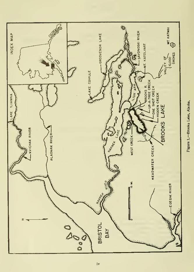
Brooks Lake is located on the Alaska

Peninsula 45 miles east of Bristol Bay (fig. 1).

It is about 1 1 miles long and 2 to 4 miles wide,

and flows into Naknek Lake via Brooks River.

All five species of North American salmonutilize the lake or its tributaries for spawning,

bat the sockeye ealmon, Oncorhynchus nerka

(Walbaum), is the most abundant. A significant

portion of the commercially valuable Bristol

Bay sockeye salmon run ie produced in BrooksLake and its ouilet stream. Brooks River.

The purpose of the research program at

Brooks Lake is to determine the factors that

influence abundance and survival of sockeye

salmon during their fresh-water life. Knowl-edge of these factors would assist managementof the fishery for maximum production.

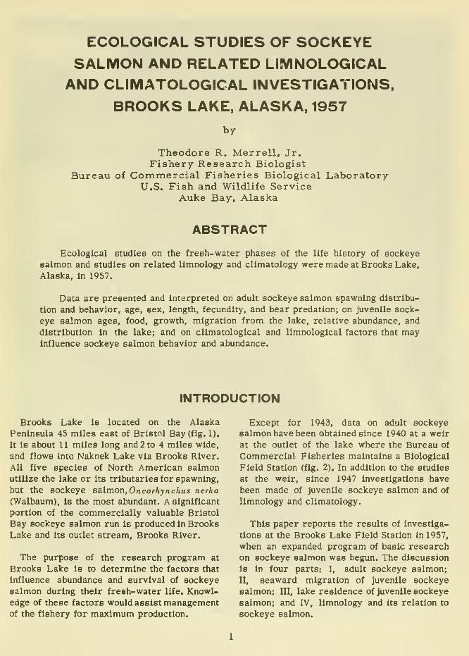
Except for 1943, data on adult sockeyesalmon have been obtained since 1940 at a weir

at the outlet of the lake where the Bureau of

Commercial Fisheries maintains a Biological

Field Station (fig. 2). In addition to the studies

at the weir, since 1947 investigations have

been made of juvenile sockeye salmon and of

limnology and climatology.

This paper reports the results of investiga-

tions at the Brooks Lake Field Station in 1957,

when an expanded program of basic research

on sockeye salmon was begun. The discussion

Is in four parts: I, adult sockeye salmon;

II, seaward migration of juvenile sockeye

salmon; III, lake residence of juvenile sockeye

salmon; and IV, limnology and its relation to

sockeye salmon.

Figure 2.-Bureau of Commercial Fisheries Biological Field Station and weir. Brooks Lake. Alaska.

PART I. ADULT SOCKEYE SALMON

The objectives of the investigations of adult

sockeye salmon were to (1) estimate numbers

of spawners; (2) determine age and length

composition, sex ratio, and fecundity of the

spawning population; (3) relate the distribution

of adults on the spawning grounds to time of

passage and abundance at the weir; (4) deter-

mine success of spawning; (5) determine rate

of disappearance of carcasses after spawning

(6) determine effects of bear predation; (7) ob-

serve spawning behavior; (8) evaluate massmovements of sockeye salmon into small tribu-

taries from the lake; and (9) evaluate the im-

portance of lake beach spawning on sockeye

salmon production of the lake.

NUMBERS OF SPAWNERS

The counting weir was installed June 18 and

was operated until October 5. It had no fixed

openings; 10 to 20 pickets were removed at

any point where fish congregated below the

weir, and fish were counted as they passed

through the gap. Multiple-unit hand tallies

were used to record both upstream and down-

stream migrants. Early in the season counters

sat on planks suspended from bipods support-

ing the weir, but since their presence dis-

turbed the fish, the counters changed and stood

in the stream several feet from the down-

stream side of the opening in the weir. To

assure good visibility, observers always wore

polarizing sun glasses.

The first migrants appeared at the weir on

June 25 when 30 were counted (fig. 3). Up-

stream migration was characterized by

one major peak within which were three

minor peaks. So that fish from the different

peaks could be recognized on the spawning

grounds, some from each peak were tagged

with Petersen disk tags with distinctive

color combinations. One combination was used

from June 25 to July 14, a second from July

14 to 19, and a third from July 19 to the end

of the migration.

On July 10 a small school of adults was

observed for the first time at the upstream

side of the weir, and as the season progressed

the school grew larger. Occasionally it moved

out of the area for several hours or would be

<cr»-

a.3

<UJcr

Wz

oo

25 30 10 20JUNE JULY

10 20 30AUGUST

Figure 3.--Daily and cumulative totals of migrating adult sockeye salmon at Brooks Lake

weir in 1957.

reduced in size for a period of days, but

the wandering fish would eventually return to

the weir area at the lake outlet. Although this

upstream school was usually quiet and seden-

tary, sometimes it would rove actively back

and forth across the face of the weir. At these

times major downstream migrations through

the counting openings in the weir were made.

These mass behavior displays could not be

related to any obvious physical feature of the

environment, and further study is needed to

explain them.

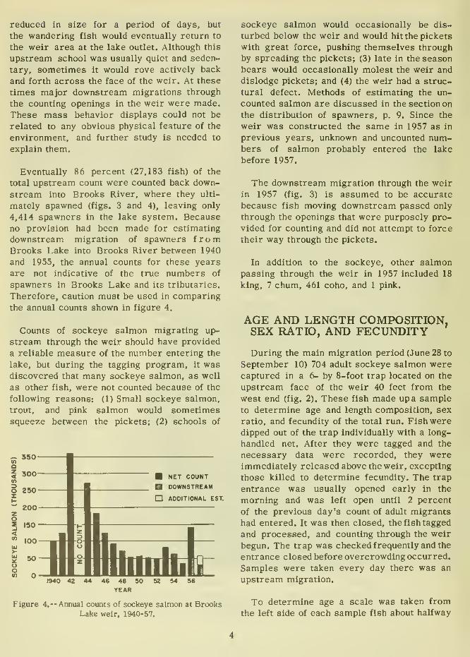
Eventually 86 percent (27,183 fish) of the

total upstream count were counted back down-

stream into Brooks River, where they ulti-

mately spawned (figs. 3 and 4), leaving only

4,414 spawners in the lake system. Because

no provision had been made for estimating

downstream migration of spawners fromBrooks Lake into Brooks River between 1940

and 1955, the annual counts for these years

are not indicative of the true numbers of

spawners in Brooks Lake and its tributaries.

Therefore, caution must be used in comparingthe annual counts shown in figure 4.

Counts of sockeye salmon migrating up-

stream through the weir should have provided

a reliable measure of the number entering the

lake, but during the tagging program, it wasdiscovered that many sockeye salmon, as well

as other fish, were not counted because of the

following reasons: (1) Small sockeye salmon,

trout, and pink salmon would sometimessqueeze between the pickets; (2) schools of

NET COUNT

DOWNSTREAM

n ADDITIONAL EST

46 48 50

YEAR

Figure 4.— Annual counts of sockeye salmon at BrooksLake weir, 1940-57.

sockeye salmon would occasionally be dis-

turbed below the weir and would hit the pickets

with great force, pushing themselves through

by spreading the pickets; (3) late in the seasonbears would occasionally molest the weir and

dislodge pickets; and (4) the weir had a struc-

tural defect. Methods of estimating the un-

counted salmon are discussed in the section on

the distribution of spawners, p. 9. Since the

weir was constructed the same in 1957 as in

previous years, unknown and uncounted num-bers of salmon probably entered the lake

before 1957.

The downstream migration through the weir

in 1957 (fig. 3) is assumed to be accurate

because fish moving downstream passed only

through the openings that were purposely pro-

vided for counting and did not attempt to force

their way through the pickets.

In addition to the sockeye, other salmonpassing through the weir in 1957 included 18

king, 7 chum, 461 coho, and 1 pink.

AGE AND LENGTH COMPOSITION,SEX RATIO, AND FECUNDITY

During the main migration period (June 28 to

September 10) 704 adult sockeye salmon werecaptured in a 6- by 8-foot trap located on the

upstream face of the weir 40 feet from the

west end (fig. 2), These fish made up a sample

to determine age and length composition, sex

ratio, and fecundity of the total run. Fish weredipped out of the trap individually with a long-

handled net. After they were tagged and the

necessary data were recorded, they wereimmediately released above the weir, excepting

those killed to determine fecundity. The trap

entrance was usually opened early in the

morning and was left open until 2 percent

of the previous day's count of adult migrants

had entered. It was then closed, the fish tagged

and processed, and counting through the weir

begun. The trap was checked frequently and the

entrance closed before overcrowding occurred.

Samples were taken every day there was an

upstream migration.

To determine age a scale was taken fromthe left side of each sample fish about halfway

between the dorsal and adipose fins and three

rows up from the lateral line. The scale wasplaced sculptured side up on a numbered spot

on a strip of gummed tape. The numbers on

the tape corresponded to numbers on water-

proof record sheets. Scales were not collected

after August 13 when scale resorption becamepronounced. Plastic impressions were later

made of the scales, using the method described

by Clutter and Whitesel (1956). Ages wereinterpreted by viewing the impressions on a

scale projector.

Most of the fish sampled (97.2 percent) werein three age categories: 52, 27 percent; Sg,

8.1 percent; and 6o, 62.1 percent. The first

numeral denotes the total age of the fish and

the subscript the number of years in fresh

water, including the brood year as 1 year. Forinstance, a 63 fish would have spent two grow-

ing seasons in fresh water and three in the sea.

Its scales would have five annuli, two formedduring its fresh-water life and three during

its ocean life.

70

60)i:5SS7CM.

50 "xn"

25 30 35 40 45 50 55 60 65 70

MIDEYE FORK LENGTH (CM.)

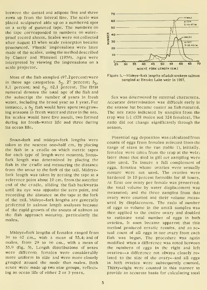
Figure 5.— Mideye-fork lengths ofadultsockeye salmonsampled at Brooks Lake weir in 1957.

Sex was determined by external characters.

Accurate determination was difficult early in

the season but became easier as fish matured.

The sex ratio indicated by samples from the

trap was 1:1 (328 males and 324 females). Theratio did not change significantly through the

season.

Snout-fork and mideye-fork lengths weretaken to the nearest one-half cm. by placing

the fish in a cradle on which metric tapes

for each type of length were mounted. Snout-

fork length was determined by placing the

fish in the cradle and measuring the distance

from the snout to the fork of the tail. Mideye-fork length was taken by zeroing the tape at a

reference point about 10 cm. from the anterior

end of the cradle, sliding the fish backwardsuntil its eye was opposite the zero point, and

recording the distance on the tape at the fork

of the tail. Mideye-fork lengths are generally

preferred in salmon length analyses because

of the rapid growth of the snouts of salmon as

the fish approach maturity, particularly the

males.

Mideye-fork lengths of females ranged from39 to 62 cm., with a mean of 55.4; and of

males, from 29 to 66 cm., with a mean of

55.9 (fig. 5). Length distributions of sexeswere different: females were considerably

more uniform in size and were more closely

grouped around the mode than males. Bothsexes were made up two size groups, reflect-

ing an ocean life of either 2 or 3 years.

Potential egg deposition was calculated fromcounts of eggs from females selected from the

range of sizes in the run (table 1). Initially,

females were taken from the trap at the weir;

later those that died in gill net sampling werealso used. To insure a full complement of

eggs, females whose ovaries were sexually

mature were not used. The ovaries werehardened in 10 percent formalin for 48 hour?.

At first one ovary per female was preserved;

the total volume by water displacement wasmeasured; and the three samples from that

ovary were counted and their volume meas-ured by displacement. The ratio of numberof eggs to volume in the small samples wasthen applied to the entire ovary and doubled

to estimate total number of eggs in both

ovaries. It soon became apparent that this

method produced erratic results, and an ac-

tual count of all eggs in one ovary from eachfish was begun. The procedure was again

modified when a difference was noted betweenthe numbers of eggs in the right and left

ovaries— a difference not always closely re-

lated to the size of the ovary— and all eggs

in both ovaries were subsequently counted.

Thirty-eight were counted in this manner to

provide an accurate basis for calculating total

egg deposition. These 38 are not included in

table 1.

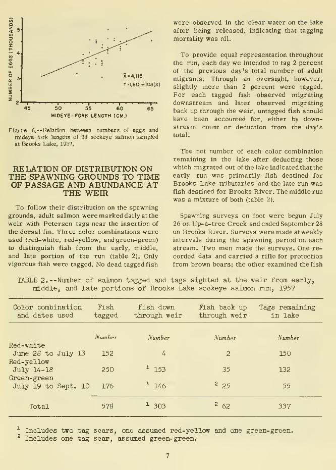
The calculated number of eggs per female

ranged from 3,044 to 5,060, with an average

of 4,115 (table 1 and fig. 6). This is con-

siderably greater than the average of 3,700

for Karluk Lake (Gilbert and Rich, 1927) and

the averages for most British Columbia races

(Rounsefell, 1957), but lower than the average

of 4,500 for Cultus Lake (Foerster, 1936). The

regression line in figure 6 was fitted by least

squares. Fecundities for fish in each length

group were read from this regression, and the

potential egg deposition of the run was then

calculated (table 1). Since the sex ratio was1:1, it was necessary only to divide the total

number of fish by two to obtain the number of

females in the lake. An estimated 14,500

female sockeye salmon in Brooks Lake and

its tributaries deposited a theoretical total

of 57 million eggs (table 1).

TABLE 1.—Potential egg deposition of sockeye salmon in Brooks Lake and Itstributaries. Calculated from fecundity data from range of sizes in the

run, June 25 to Sept. 10, 1957

Size range

inQ

inDOXI-— 4VI<DOUJ

q:iij

oz

X = 4,II5

Y=I.80I+ I03(X)

45—r-50 55 60

MIDEYE-FORK LENGTH (CM.)

65

Figure 6.-- Relation between numbers of eggs and

mideye- fork lengths of 38 sockeye salmon sampled

at Brooks Lake, 1957.

RELATION OF DISTRIBUTION ONTHE SPAWNING GROUNDS TO TIMEOF PASSAGE AND ABUNDANCE AT

THE WEIR

To follow their distribution on the spawning

grounds, adult salmon were marked daily at the

weir with Petersen tags near the insertion of

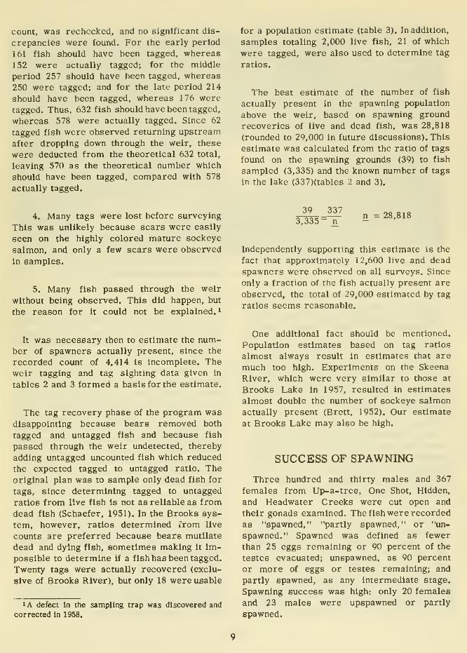
the dorsal fin. Three color combinations wereused (red-white, red-yellow, and green-green)

to distinguish fish from the early, middle,

and late portion of the run (table 2). Only

vigorous fish were tagged. No dead tagged fish

were observed in the clear water on the lake

after being released, indicating that tagging

mortality was nil.

To provide equal representation throughout

the run, each day we intended to tag 2 percent

of the previous day's total number of adult

migrants. Through an oversight, however,

slightly more than 2 percent were tagged.

For each tagged fish observed migrating

downstream and later observed migrating

back up through the weir, untagged fish should

have been accounted for, either by down-stream count or deduction from the day's

total.

The net number of each color combination

remaining in the lake after deducting those

which migrated out of the lake indicated that the

early run was primarily fish destined for

Brooks Lake tributaries and the late run wasfish destined for Brooks River. The middle run

was a mixture of both (table 2).

Spawning surveys on foot were begun July

26 on Up-a-tree Creek and ended September 28

on Brooks River. Surveys were made at weekly

intervals during the spawning period on each

stream. Two men made the surveys. One re-

corded data and carried a rifle for protection

from brown bears; the other examined the fish

TABLE 2.—Number of salmon tagged and tags sighted at the weir from early,

middle, and late portions of Brooks Lake sockeye salmon run, 1957

Color combination

carcasses. On surveys in brushy areas,

whistles were blown every few minutes to

alert the bears; if they heard our approach the

bears usually avoided us. Polaroid glasses

were used to insure maximum and comparablevisibility for all surveys. In addition to sur-

veys on foot, three surveys were made fromthe air. Table 3 summarizes the sightings madeon surveys. Of the aerial surveys, only the

one on Headwater Creek was used to estimate

numbers of fish.

Although tagging 2 percent of the fish passing

the weir should have resulted in a 1:50 ratio

of tagged to untagged fish in the population

above the weir, the number of tagged fish in

samples was always less than expected. Five

possible explanations for this discrepancy

are:

1. Tagged fish suffered a heavier mor-tality than untagged fish. This can be dismissedbecause there was no evidence of tagged fish

dying before spawning.

2. Tagged fish behaved differently fromuntagged fish, resulting in biased samples.

This is not likely since there was never any

evidence of high concentrations of tagged fish

in locations where schools were visible. Atagging experiment on Hidden Creek in 1949

further substantiated this conclusion (Eicher,

1951).

3. Calculations for each day's tagging

were incorrectly made. On the basis of the

observed count, this was not a factor. Eachday's tagging, based on the previous day's

TABLE 3. —Summary of sockeye salmon sighted and fin clipped by observers onstream and aerial surveys. Brooks Lake system, July 26 to September 28, 1957

Locationand numberof surveys

Livefish

Dead fin-clippedfish

count, was rechecked, and no significant dis-

crepancies were found. For the early period

161 fish should have been tagged, whereas

152 were actually tagged; for the middle

period 257 should have been tagged, whereas

250 were tagged; and for the late period 214

should have been tagged, whereas 176 were

tagged. Thus, 632 fish should have been tagged,

whereas 578 were actually tagged. Since 62

tagged fish were observed returning upstream

after dropping down through the weir, these

were deducted from the theoretical 632 total,

leaving 570 as the theoretical number which

should have been tagged, compared with 578

actually tagged.

for a population estimate (table 3). In addition,

samples totaling 2,000 live fish, 21 of which

were tagged, were also used to determine tag

ratios.

The best estimate of the number of fish

actually present in the spawning population

above the weir, based on spawning ground

recoveries of live and dead fish, was 28,818

(rounded to 29,000 in future discussions). This

estimate was calculated from the ratio of tags

found on the spawning grounds (39) to fish

sampled (3,335) and the known number of tags

in the lake (337)(tables 2 and 3).

4. Many tags were lost before surveying

This was unlikely because scars were easily

seen on the highly colored mature sockeye

salmon, and only a few scars were observed

in samples.

5. Many fish passed through the weir

without being observed. This did happen, but

the reason for it could not be explained. *

39 3373,335- n

n = 28,818

Independently supporting this estimate is the

fact that approximately 12,600 live and dead

spawners were observed on all surveys. Since

only a fraction of the fish actually present are

observed, the total of 29,000 estimated by tag

ratios seems reasonable.

It was necessary then to estimate the num-ber of spawners actually present, since the

recorded count of 4,414 is incomplete. Theweir tagging and tag sighting data given in

tables 2 and 3 formed a basis for the estimate.

The tag recovery phase of the program was

disappointing because bears removed both

tagged and untagged fish and because fish

passed through the weir undetected, thereby

adding untagged uncounted fish which reduced

the expected tagged to untagged ratio. Theoriginal plan was to sample only dead fish for

tags, since determining tagged to untagged

ratios from live fish Is not as reliable as from

dead fish (Schaefer, 1951). In the Brooks sys-

tem, however, ratios determined irom live

counts are preferred because bears mutilate

dead and dying fish, sometimes making it im-

possible to determine if a fish has been tagged.

Twenty tags were actually recovered (exclu-

sive of Brooks River), but only 18 were usable

1 A defect In the sampling trap was discovered and

corrected in 1958.

One additional fact should be mentioned.

Population estimates based on tag ratios

almost always result in estimates that are

much too high. Experiments on the Skeena

River, which were very similar to those at

Brooks Lake in 1957, resulted in estimates

almost double the number of sockeye salmon

actually present (Brett, 1952). Our estimate

at Brooks Lake may also be high.

SUCCESS OF SPAWNING

Three hundred and thirty males and 367

females from Up-a-tree, One Shot, Hidden,

and Headwater Creeks were cut open and

their gonads examined. The fish were recorded

as "spawned," "partly spawned," or "un-

spawned." Spawned was defined as fewer

than 25 eggs remaining or 90 percent of the

testes evacuated; unspawned, as 90 percent

or more of eggs or testes remaining; and

partly spawned, as any Intermediate stage.

Spawning success was high: only 20 females

and 23 males were upspawned or partly

spawned.

RATE OF DISAPPEARANCE OFCARCASSES AFTER SPAWNING

Carcasses of fish found on each survey weredistinctively marked by amputating one or more

of the fins and were replaced where they were

found. Any fin-clipped fish found on a survey

was recorded. Despite the fact that surveys

were made at 7-day intervals and 3,378

carcasses were marked, only 41, or 1 percent,

were subsequently found, indicating a rapid

disappearance (table 3). On the smaller tribu-

taries scavengers seemed to be responsible,

while on Brooks River the fast current caused

carcasses to be washed downstream into deep

water. The successive survey counts of dead

fish on a given stream may therefore be re-

garded as additive for minimum total enumera-

tion purposes.

EFFECTS OF BEAR PREDATION

Bears were numerous and fed actively on

salmon in all tributariesof Brooks Lake during

the early and peak spawning periods. Towardthe end of spawning in each stream, despite

an abundance of salmon, bears moved to

berry fields on high ground away from the

stream valleys. This seasonal shift in diet

from salmon to berries has been described

at Karluk Lake on Kodiak Island by Clark

(1957). Our program in 1957 was not originally

planned to study bear predation, but someknowledge was gained.

From the evidence of fresh signs of bears

(feces, footprints, clawmarks) and of partially

eaten salmon carcasses, bear activity in order

of prevalence by stream was as follows: Hidden

Creek, Up-a-tree Creek, One Shot Creek,

Headwater Creek, and Brooks River.

Bears could be heard from the streamsidefield station on Brooks River almost every

night during September as they fought with

each other and pursued salmon near the weir.

This was a temporary situation, however,

resulting from the concentration of fish and

the presence of the weir, which prevented fish

from escaping easily. Under natural conditions

bears probably have little effect on sockeye

salmon in large streams such as HeadwaterCreek and Brooks River.

Hidden Creek, the most heavily frequented

by bears, was carefully surveyed on September

3 to evaluate the effect bears had on spawning.

The creek, about 10 feet wide and flowing

about 10 cubic feet per second, is similar

in size and terrain to Up-a-tree and One Shot

Creeks. The creek was surveyed upstream to

beyond the limit of spawning. Most of the banks

were covered with brush and high grass, but

every 10 or 15 feet the vegetation was flattened,

indicating "feeding tables" where bears had fed

on salmon. It could not be determined if these

were the result of fishing by many bears or

of great activity by a few. Fresh bear feces

was abundant and contained both berries and

salmon bones.

Most of the carcasses mutilated by bears

had deep tooth marks, or the posterior section

of the body was missing (fig. 7). On the Hidden

Creek survey, several live spent salmon wereseen with large bite marks on the median and

posterior portions of the body. Spawning suc-

cess was recorded whenever it was possible.

The appearance of the gonads in the anterior

portion of the body usually provided clues to

whether fish had spawned successfully.

Of 290 dead sockeye salmon found on the

Hidden Creek survey, 188 were females and 102

males. Bears had mutilated 247, of which 10

females and 9 males were unspawned, and 3

females and 13males were partly spawned. Theremaining 212 fish were completely spawned.

Spawning was apparently at or slightly past its

peak, since more carcasses (489) were found on

this survey than on any preceding or succeeding

survey. Although this was only a single sample

from one stream. I believe it is a measure of

maximum bear damage on the Brooks system.

The spawning population in Hidden Creek wasmore heavily affected by bears than the popu-

lations in the other tributaries, as shown by

comparative general observations of bear

predation during stream surveys.

I conclude that even under conditions of

intense bear activity on a small stream where

salmon are abundant and vulnerable, bears

catch mostly spawned out fish and have little

effect on ultimate production.

10

^'^^rs:

Figure 7.— Bear-mutilated sockeye salmon found alive on survey of Hidden Creek in 1957.

SPAWNING BEHAVIOR

An important objective of the 1957 programwas to learn some basic facts about sockeye

salmon spawning behavior in the Brooks sys-

tem. On Brooks River, 400 yards below the

lake, observations were made daily fromAugust 16 through October 7 (except for 6 days)

from a portable 20-foot high aluminum scaf-

fold. The tower overlooked a gravel riffle

used extensively for spawning. A grid system(fig. 8) was constructed over the area to

facilitate location of redds and to orient

spawning observations by reference points.

The area was 75 feet wide (the width of the

river) and 285 feet long and was portioned

into 15-foot squares. The portioning was ac-

complished by driving aluminum weir pickets

at 15-foot intervals on each bank of the river

and tying lines between them; then small

colored cloth strips were tied to the lines at

15-foot intervals, dividing each row into five

sections. Rows were assigned numbers, and

the five sections within the rows were also

numbered. Each of the five sections was visu-

ally segregated into an imaginary quadrat.

An abbreviated code was used to indicate a

desired point: For example, R.S B referred

to row 6, section 2, the upper right quadrat.

Sections 12 through 15 of the grid (fig. 8)

were used to test the hypothesis that stream

bottoms with loose gravel are used more by

spawning fish than stream bottoms with com-pact gravel. Alternate 7|-foot-wide strips

of gravel in rows 12 through 15 were loosened

with a hand shovel before the onset of spawn-

ing. The positions of redds within this area

on 3 different days were as follows:

4

loosened by gravel removal operation, bull-

dozing in streambeds, or fording by vehicles.

At Brooks Lake, however, the preference for

such areas was small. Perhaps under condi-

tions of severe gravel compaction and sparse

spawning populations, it would be greater.

To ensure consistent methods and com-parable results throughout an observation

period, personnel followed the procedures

outlined below.

1. To avoid disturbing fish en route to the

tower from the field station, the observer

crossed the stream at least 100 yards above

the study area and then walked on the bank

until reaching the tower.

2. To preclude recording behavior that

might be influenced by the observer as he

climbed the tower, 5 minutes elapsed before

observations were recorded.

3. Observations were made of one row at

a time for 5-minute periods and were con-

fined to rows 7, 8, 9, and 10 after August 31.

These limitations were adopted when it becameapparent that a single observer could effec-

tively observe only a limited area wherevisibility was best.

4. Sex ratios on all redds were noted at

the start of each day's observations.

5. Records of individual fish behavior by

sex were usually confined to defense activity

over redds with a 1:1 sex ratio.

6. A code was devised to simplify and

expedite observations and recording. The code

was based on three categories of activity that

were encountered most frequently as follows:

Male or

female

activity

TABLE 4.—Observations of activity of spawning sockeye salmon from counting towers on Brooks River,

Just below outlet of Brooks Lake, August 16 to October 7, 1957

by the drop in lake level was a 10° F. de-

crease in stream temperature at the outlet

of the lake. These factors apparently tem-

porarily upset the normal behavior of the

spawning salmon. No relationship could be

demonstrated between spawning peaks and daily

water level, flow, or temperature.

As the season progressed, the number of

spawned females unaccompanied by males

increased consistently, reaching a peak by

October 1, 7 days after the final spawning

peak. This phenomenon was a reflection of

the longer life of females after completion

of spawning. Females continued to guard the

redd aggressively after completing spawning

and until they died.

The upstream counts of sockeye salmon at

the weir (fig. 3) indicate a trimodal pattern

similar to that indicated by spawning activity

in the observation area (fig. 9). Tagging data,

however, show that the first wave in weir

counts included very few Brooks River fish.

Most Brooks River fish that subsequently

returned downstream through the weir werefrom the second and third waves of upstreamweir counts. 1 conclude that migration Into

Brooks Lake, as indicated by weir counts,

was not closely related to the spawning wavesin Brooks River, but a definite relationship

was detected between migration downstreamfrom the lake at the weir and the spawning

waves. The August 26 spawning wave waspreceded by a peak downstream movementun August 6; the Septemlier 7 wave by the

September li peak; and the September 24 waveby the September 18 peak. Neither the period

of precedence nor the comparative magnitude

are consistent, liui tiiis relatit)naliip lieiween

downstream migration from the lake and

peaks of spawning in Brooks River (and

results of tagging at the weir) prove that

many of the sockeye salmon included in tlie

counts at Brooks weir are from the Brooks

River stock.

l^'rom the 1957 data I hypothesize two pos-

sible kinds ol causative factors responsible for

this wave pattern of nuiss spawning: The time

of spawning Is governed by an endogenous fac-

tor somehow related to the time spt-nt In fresh

water or by an exogenous environmental factor

that induces sockeye salmon to spawn during

successive periods. If the first hypothesis is

true, fish must migrate from the ocean in waves

timed similarly to spawning waves. In 1957

we had no means of verifying this. If the second

hypothesis is true, we should be able to recog-

nize the influencing factors by careful study

and observation. In 1957 none of the exogenous

environmental factors measured appeared to

influence spawning, with the possible exception

of competition for spawning space.

The behavior of individual sockeye salmon

in the observation area was found to follow

certain well-defined patterns closely asso-

ciated with the three spawning waves. Thesequence of behavior through a spawning wasgenerally as follows:

1. Groups of 10 to 50 sockeye salmon,

predominantly males, moved upstream fromdeep pools onto spawning riffles. The mostdistinctive behavior pattern noted was what

we termed a "sidling bluff." This started

when two males about the same size movedtoward each other until they were side by

side. They then swam diagonally across the

stream, eye-to-eye. When one bank wasreached, they quickly reversed positions and

sidled back to the other bank where the process

was repeated. After several trips back and

forth, one of the males began to give ground.

The bluffing was ended with the victor crowding

the loser until the loser fled downstream to

escape. No biting or other violence was evi-

dent during the sidling bluff nor were females

ever involvetl.

2. A pair of fish would establish a redd

in a location not strongly defended by another

female. When many fish were present, a

female was often chased from place to place

before finding an undefended site.

3. Small males (jack salmon) actively

tried to establish iheniselves with a female

during the redd site-seeking stage. They

were never observed succeeding, always being

forced away by a larger male.

4. Large females were most sought by

tlu- males, resulting in ihe largest and mostpowerful males spawning with the largest

15

females, and the smaller males spawning with

the smaller females.

5. Jack salmon constantly attempted to

infiltrate an established redd but were driven

away by both males and females, usually

by the males. As a wave of spawning waned,

jack salmon finally gained brief access to

redd territories.

6. The male often took an active part in

digging the redd but dug more sporadically

than the female.

males. The instant a fresh newcomer started

a digging movement, all spawned-out females

in the vicinity converged in a concerted attack.

Perhaps this behavior is a protective instinct

to prevent disturbing existing redds.

9. At the peak of spawning and for a day

or two after, dead and dying spent males wereobserved floating through the spawning area.

The floating carcasses were almost never

females. Spawning fish paid no attention to

these carcasses even when they entered a

defended redd area.

7. Males chased mostly males and fe-

males mostly females. This phenomenon would

tend to make full use of a spawning stock

with an unbalanced sex ratio. For instance, if

there were a surplus of females, a male

would be able to spawn with many females

without interference, as demonstrated in con-

trolled experiments at Wood River Lakes by

Mathisen (1955). Of 134 females chased froman established redd with a 1;1 sex ratio, only

16 were chased by males.

8. As a spawning wave waned, the numberof lone females increased rapidly (0:1 sex

ratio), and males, which died first, disappeared

(fig. 9). Lone females on completed redds

were very intolerant of digging by new fe-

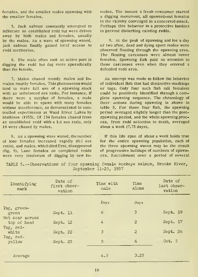
An attempt was made to follow the behavior

of individual fish that had distinctive markings

or tags. Only four such fish (all females)

could be positively identified through a com-plete spawning sequence. The chronology of

their actions during spawning is shown in

table 5. For these four fish, the spawning

period averaged slightly longer than the post-

spawning period, and the whole spawning proc-

ess, from redd selection to death, averaged

about a week (7.75 days).

If this life span of about a week holds true

for the entire spawning population, each of

the three spawning waves may be the result

of progressive buildups of numbers of spawn-

ers. Recruitment over a period of several

TABLE 5. — Observations of four spawning female sockeye salmon. Brooks River,

September 11-25, 1957

Identifyingmark

Date offirst obser-

vation

Time withmale

Timealone

Date oflast obser-

vation

Tag, green-green

Net scar acrosstop of head

Tag, red-white

Tag, red-yellow

Sept. 11

Sept. 12

Sept. 22

Sept. 25

Days

6

Ar

3

5

Days

3

2

2

6

Sept. 19

Sept. 17

Sept. 26

Oct. 5

Average 4.5 3.25

16

days until maximum density for that wave

has been reached would explain the shape of

the curve comprising each of the 2-week-long

peaks (fig. 9).

the bears caused a mass evacuation of the

stream and return to the relative safety of

the lake.

MASS MOVEMENTS OF SPAWNINGSOCKEYE SALMON FROM

BROOKS LAKE

Since mass movements of salmon fromBrooks Lake to One Shot Creek and back

to the lake had been reported in previous

years, we set up a 10-foot tower near the

mouth of the creek to observe upstream and

downstream migrations. The first small school

of salmon was seen July 24. The school

gradually increased in size and between Aug-ust 16 and 20 milled about the mouth of OneShot Creek. On August 21 the school entered

the stream and migrated upstream to spawn.

A diurnal movement of salmon in and out

of Hidden Creek was observed on August 6.

During the afternoon of August 5, a large

school was in the lake off the mouth of the

creek. On the morning of the 6th the school

was still there, and no fish were in the creek.

At 1 p.m. several hundred ascended the

creek for 500 yards, but at 2 p.m. they all

turned suddenly and descended to the lake.

Their return to the lake coincided with the

appearance of two bears in the stream 400yards above the mouth. By 4 p.m. only a fewfish remained in Hidden Creek, and these werenear the mouth. Apparently the appearance of

LAKE BEACH SPAWNING

Sockeye salmon are known to spawn on suit-

able beaches in many areas, and spawning

has been reported along the beach of BrooksLake between the outlet and Up-a-tree Creek(Richard Straty, personal communication).

From mid-July until mid-September, we sur-

veyed the gravelly beaches in shallow water

around the Brooks Lake shoreline from boats.

On September 14 during an aerial reconnais-

sance of the lake shoreline, we saw several

hundred sockeye salmon spawning in shallow

water along a mile of beach north of the

mouth of Up)-a-tree Creek. The same area

was surveyed by boat on 3 days with the

following results:

Date

September 15

September 22

October 4

Numberof adults

357

278

59

Numberof redds

146

Not counted

136

Since the fish and redds were clearly visible

in the shallow water, the maximum count

may be regarded as a close approximation

of the total numbers of beach spawners.

Beach spawning was a minor factor in BrooksLake production in 1957.

PART II. JUVENILE SOCKEYE SALMON SEAWARD MIGRATION

In the spring juvenile sockeye salmon'migrate to the sea from their lake nursery

area where they have spent the previous 1 or

2 years. This migration provides an oppor-

'I define juvenile salmon as any young salmon. In

the life history stage between hatching and migrationto the sea. Fry are salmon In their first year of life.

Including the period between hatching and the first

winter. Yearlings are salmon in their second year of

life. Including the period between the first and secondwinters. Two-year-olds are salmon in their third yearof life, between the second and third winters.

tunity to evaluate survival from the parent

run and to study characteristics of the sea-

ward migration.

Five aspects of the seaward migration of

juvenile sockeye salmon were investigated at

Brooks Lake in 1957: (1) Age and length

composition of seaward migrants; (2) seasonal

length-weight relationship of juvenile migrantsby age groups; (3) characteristics of daily and

seasonal migration by age group of sockeye

salmon and of other species migrating out of

the lake; (4) migration of Juveniles upstream

17

from Brooks River into Brooks Lake;

(5) migratory behavior of juveniles.

and

AGE AND LENGTH OF SEAWARDMIGRANTS

To assess relative abundance, samples of

juveniles were captured with fyke nets during

the downstream migration. No attempt wasmade to estimate total migration. Three nets

were fished nightly at the lake outlet during

periods of heavy migration, one near each

shore and one in midriver (figs. 10 and 11).

Usually the nets were fished for only an hour

a night, but five 24-hour and five all-night

samples were also taken. After June 1 1 whenthe migration tapered off, only one net (no. 1,

fig. 10) was fished, and the sampling schedule

was changed from every night to every third

night or less.

BROOKS LAKE

Figure 10. --Locations of fyke nets at Brooks Lakeoutlet, 1957.

Only portions of each nightly catch wereusually processed: from May 21 to 31 (except

for all-night samples) about 20 fish per net;

from June 1 to 11, 5 fish per net; and from

June 17 to October 1, 20 fish per net excepting

the June 1-11 period, on nights when the total

catch per net was less than 20 fish, the entire

catch was processed.

Figure ll.--Fyke nets and method of collecting juvenile sockeye salmon at Brooks Lake outlet, 1957.

18

Randomness of samples was assured by suc-

cessively separating a net's catch of live

juveniles in a washtub into equal parts with

a mesh panel and releasing half of the fish

each time until the desired number remained.

Ages of 807 fish were read in the field fromscales dry-mounted between two microscope

slides. An additional 2,287 fish were aged

on the basis of estimated length alone, as de-

scribed later. Annuli criteria were established

by examination and by methods described by

Clutter and Whitesel (1956), Each scale wasread once after which 49 scales were selected

at random and read a second time without

reference to the first reading. Agreementbetween first and second readings was 100

percent. Although reading scales from samplescollected at the end of the summer was com-plicated by early formation of an annulus in

September, close agreement was attained in

independent readings by two readers. Forklengths were measured to the nearest milli-

meter.

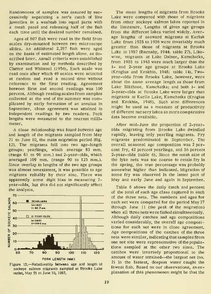
A close relationship was found between age

and length of the migrants sampled from May21 to June 10, the main migration period (fig.

12). The migrants fell into two age-length

groups: yearlings, which average 83 mm.(range 61 to 96 mm.) and 2-year-olds, which

averaged 109 mm. (range 90 to 125 mm.).

Since overlap in lengths of the two age groups

was almost nonexistent, it was possible to age

migrants reliably by their size. There wasapparently some digit bias in measuring 2-

year-olds, but this did not significantly affect

the analysis.

70-

CO

60- YEARUMS*

50-

(nc|92)

i- 82.7 mn.

40->-UJ

uom 30-

D 2-YEAR-OLOS

(l<:382)

i = l09.0 mm.

20-

10-

0-^60 70£sjm ^

80 90 100 no 120

FORK LENGTH (MM)

Figure 12.— Relationship between age and length of

sockeye salmon migrants sampled at Brooks Lake

outlet. May 21 to June 10, 1957.

The mean lengths of migrants from BrooksLake were compared with those of migrants

from other sockeye salmon lakes reported in

the literature. Lengths of given age groups

from the different lakes varied widely. Aver-

age lengths of seaward migrants at Karluk

Lake from 1925 to 1936 were invariably muchgreater than those of migrants at BrooksLake in 1957 (Barnaby, 1944: table 27). Like-

wise, migrants at Lake Dalnee, Kamchatka,

from 1935 to 1943 were much larger than the

1- and 2-year age groups at Brooks Lake(Krogius and Krokhin, 1948: table 14). Two-year-olds from Brooks Lake, however, wereabout the same average length as those fromLake Blizhnee, Kamchatka; and both 1- and

2-year-olds at Brooks Lake were larger than

migrants at Kurile Lake, Kamchatka (Krogius

and Krokhin, 1948). Such size differences

might be used as a measure of productivity

of different nursery lakes as more comparativedata become available.

After mid-June the proportion of 2-year-olds migrating from Brooks Lake dwindled

rapidly, leaving only yearling migrants. Frymigrants predominated in September. Theoverall seasonal age composition was 2 per-

cent fry, 42 percent yearlings, and 56 percent

2-year-olds (table 6). Since the mesh size of

the fyke nets was too coarse to retain fry in

the spring, the true percentage was probably

somewhat higher than indicated. Migration of

some fry was observed in the latter part of

May and early June and again in September.

Table 6 shows the daily catch and percent

of the total of each age class captured in each

of the three nets. The numbers and ages for

each net were compared for the period May 27

through June 11 (the peak of the migration)

when all three nets were fished simultaneously.

Although daily catches and age compositions

varied considerably, the overall age composi-tions for each net were in close agreement.Age compositions of the catches of the three

nets were similar, indicating that samples fromone net site were representative of the popula-

tions sampled at the other two sites. Thecatches were inversely proportional to the

amount of water strained—the largest net (no.

2) in the fastest, deepest water caught the

fewest fish. Based on our observations, an ex-

planation of this phenomenon might be that the

19

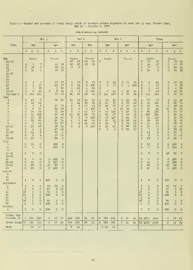
TABLE 6. --Number and percent of total dally catch of sockeye salmon migrants in each net by age, Brooks Lake,May 20 - October 1, 1957

[Fish of unknown age excluded]

migrants followed the lake shores on each side

of the outlet stream, thereby being concentrated

along the stream-banks where the smaller

shore nets were located.

From June 1 to 11, to determine if small

samples from each net's total nightly catch

would yield representative age data, ages of

approximately five fish from each net's catch

per night were compared with ages of the total

catch of each net (table 7). The randommethod of sample selection described pre-

viously was used.

Differences in age between small samples

and total catches on individual days werequite large; however, age composition fromthe small samples was identical with the over-

all age composition from the entire catch

for the period from May 27 to June 11

(table 6), and was only 3 percent different

from the total sample of the period June 1-11

(table 7). Small samples were therefore ade-

quate for determining age composition for the

season but not for individual days.

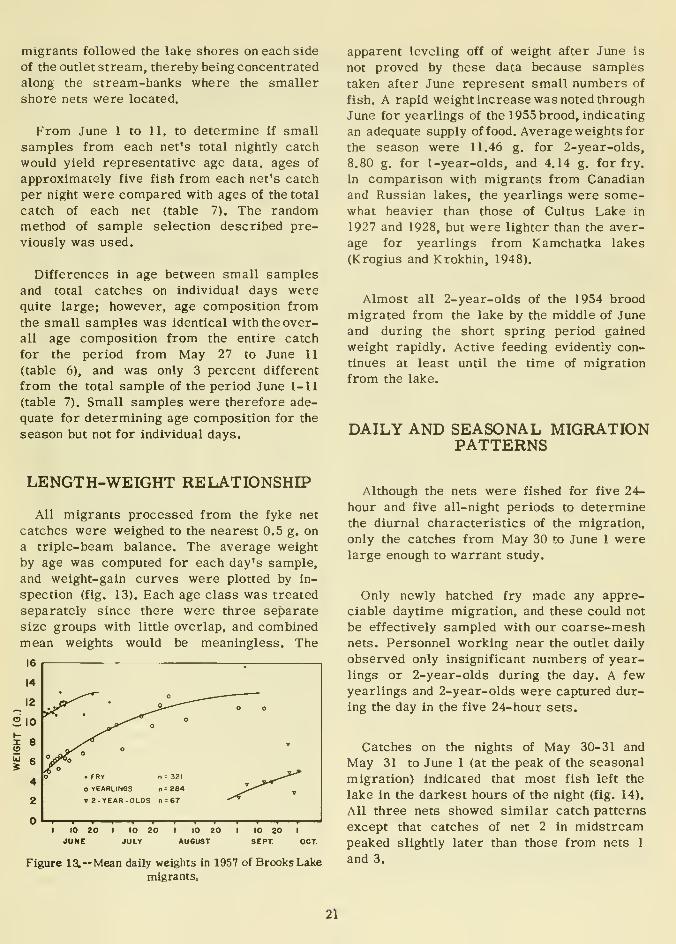
apparent leveling off of weight after June is

not proved by these data because samples

taken after June represent small numbers of

fish. A rapid weight increase was noted through

June for yearlings of the 1955 brood, indicating

an adequate supply of food. Average weights for

the season were 11.46 g. for 2-year-olds,

8.80 g. for 1-year-olds, and 4.14 g. for fry.

In comparison with migrants from Canadian

and Russian lakes, the yearlings were some-what heavier than those of Cultus Lake in

1927 and 1928, but were lighter than the aver-

age for yearlings from Kamchatka lakes

(Krogius and Krokhin, 1948).

Almost all 2-year-olds of the 1954 brood

migrated from the lake by the middle of June

and during the short spring period gained

weight rapidly. Active feeding evidently con-

tinues at least until the time of migration

from the lake.

DAILY AND SEASONAL MIGRATIONPATTERNS

LENGTH-WEIGHT RELATIONSHIP

All migrants processed from the fyke net

catches were weighed to the nearest 0.5 g. on

a triple-beam balance. The average weight

by age was computed for each day's sample,

and weight-gain curves were plotted by in-

spection (fig. 13). Each age class was treated

separately since there were three separate

size groups with little overlap, and combined

mean weights would be meaningless. The

16

I 10 20AueusT

10 20 I

SEPT. OCT

Figure 13.— Mean daily weights In 1957 of Brooks Lake

migrants.

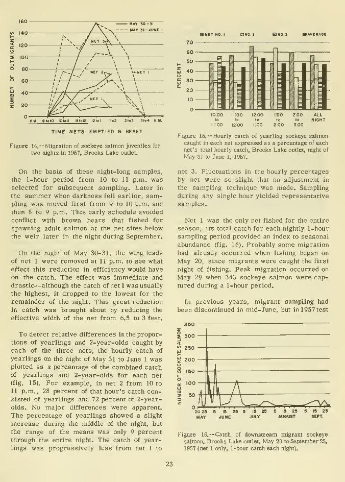
Although the nets were fished for five 24-

hour and five all-night periods to determine

the diurnal characteristics of the migration,

only the catches from May 30 to June 1 werelarge enough to warrant study.

Only newly hatched fry made any appre-

ciable daytime migration, and these could not

be effectively sampled with our coarse-meshnets. Personnel working near the outlet daily

observed only insignificant numbers of year-

lings or 2-year-olds during the day. A few

yearlings and 2-year-olds were captured dur-

ing the day in the five 24-hour sets.

Catches on the nights of May 30-31 and

May 31 to June 1 (at the peak of the seasonal

migration) indicated that most fish left the

lake in the darkest hours of the night (fig. 14).

All three nets showed similar catch patterns

except that catches of net 2 in midstreampeaked slightly later than those from nets 1

and 3.

21

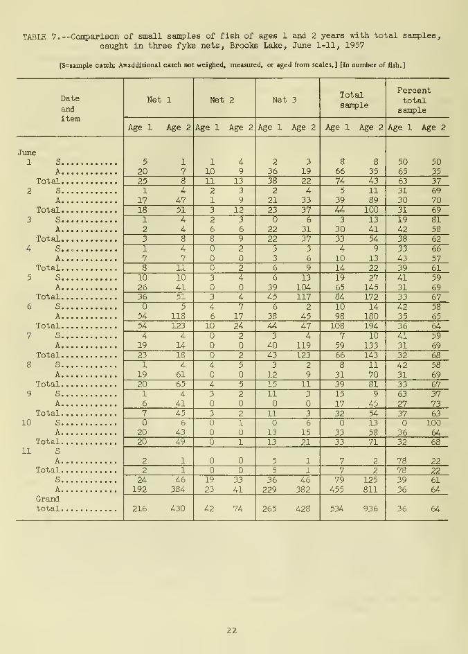
TABLE 7.—Comparison of small samples of fish of ages 1 and 2 years with total san^sles,

caught in three fyke nets. Brooks Lake, June 1-11, 1957

[S=sample catch; A=additional catch not weighed, measured, or aged from scales.] [In number of fish.]

Date

and

160

<ITe

3O

o

bJm

PM 9tolO lOtoll ntolZ l2tol lIoZ 2to3 3ta4 A.M.

TIME NETS EMPTIED S RESET

Figure 14.--Migration of sockeye salmon juveniles for

two nights in 1957, Brooks Lake outlet.

BNO.S

10.00

fishing continued throughout the summer. Asecond major migration took place on June 28,

and smaller migrations during the last of

July and the middle of September. A few sock-

eye salmon migrated from the lake through

the summer. Future programs requiring an

estimate of total migration should take into

consideration an extended migration period

throughout the summer and fall. It is not

known whether these summer migrants re-

mained in Naknek Lake until the following

spring, or whether they migrated immediately

to the sea.

In addition to juvenile sockeye salmon seven

other species of fish were caught in the nets;

881 sculpins (Cotius spp.); 57 coho salmon

(Oncorhynchus kisutch); 23 rainbow trout(Salmo gairdneri); 9 Dolly Varden (Salvelinus

malma); 4 brook lamprey (Entosphenus lamottei);

15 blackfish (DalUapectoralisj; and 22 nine-

spine stickleback (Pungitius pungitius). Almostall of the catches of these species were madeat night. The coho salmon were caught fromJune 2 through 29, and some daytime migration

of this species was observed by personnel

counting adult sockeye salmon at the weir

through June and July. Rainbow trout migrated

sporadically from June 4 until October, and

Dolly Varden first appeared at the end of

September. A few lampreys were evident

during May and early June, and blackfish

appeared late in the summer. A few stickle-

backs and large numbers of sculpins were

caught intermittently throughout the sum-mer.

By the very nature of Brooks River this

is not likely to happen. In the first place,

juveniles attempting to swim from lower

Brooks River or Naknek Lake would encounter

Brooks Falls, which is about 8 feet high. Anefficient gravity flow fish ladder enables adult

salmon to bypass the falls, but it would be

extremely difficult for juveniles to do so.

Furthermore, several stretches of Brooks

River have rapids so swift that it is difficult

for a man to keep his footing.

Although it was deemed unlikely that small

salmon, particularly fry, could migrate up-

stream, a stationary trap was constructed to

intercept a portion of small fish that might

do so and so provide a measure of the serious-

ness of the problem. The trap was located on

a small point of land about 100 yards below the

outlet of Brooks River on the right bank

(fig. 17). It was simply constructed with two

rigid leads of 1/4-inch-mesh wire cloth trap

and a box trap of 3/8-inch-mesh wire cloth

lined with 1/8-inch-mesh nylon bobbinet. Onelead intersected the shore at an angle, and

the other extended toward midstream where

the current was too swift for fry to swimupstream. We assumed that small fish attempt-

ing an upstream migration would seek a path

of least resistance along the shore. The trap

was usually emptied and cleaned twice daily.

Fish entering the trap eventually escaped, but

a relative index of migration was obtained

from fish remaining in the trap at the time

of checking. The trap was installed June 2 and

removed September 14. The catch by month

is shown in table 8.

MIGRATION OF JUVENILESALMON UPSTREAM

The question had been raised as to whether

juvenile sockeye salmon originating in BrooksRiver or Naknek Lake might migrate upstreaminto Brooks Lake. Such a phenomenon has

been noted at some lakes, notably Karluk

Lake on Kodiak Island, Alaska, and Babine

Lake in British Columbia (Roy Jackson, per-

sonal communication). An upstream migration

on a large scale at Brooks Lake would seri-

ously complicate studies of survival and pro-

duction of the indigenous lake population.

Three features of the trapping study are of

particular interest: (1) The maximum catch of

sockeye fry (244) was in July but was insigni-

ficant compared with the total probable down-

stream migration from Brooks Lake; (2) the

catch of fry in June was small despite the fact

that maximum downstream migration was

observed during this period; and (3) threespine

stickleback (Gastemsteus aculeatus) and nine-

spine stickleback, which do not usually occupy

the same waters, were captured together.

Observations of Brooks River incidental to

other activities supported the conclusion that

the upstream migration of sockeye salmon

24

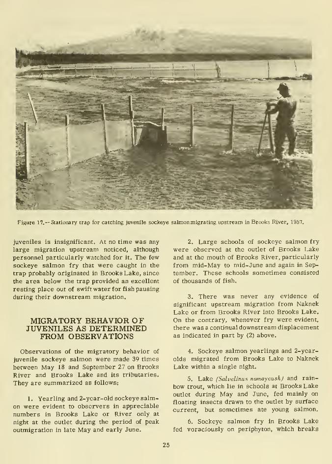
Figure 17.— Stationary trap for catching juvenile sockeye salmon migrating upstream in Brooks River, 1957.

juveniles is insignificant. At no time was any

large migration upstream noticed, although

personnel particularly watched for it. The few

sockeye salmon fry that were caught in the

trap probably originated in Brooks Lake, since

the area below the trap provided an excellent

resting place out of swift water for fish pausing

during their downstream migration.

MIGRATORY BEHAVIOR OFJUVENILES AS DETERMINED

FROM OBSERVATIONS

2. Large schools of sockeye salmon fry

were observed at the outlet of Brooks Lake

and at the mouth of Brooks River, particularly

from mid-May to mid-June and again in Sep-

tember. These schools sometimes consisted

of thousands of fish.

3. There was never any evidence of

significant upstream migration from Naknek

Lake or from Brooks River into Brooks Lake.

On the contrary, whenever fry were evident,

there was a continual downstream displacement

as indicated in part by (2) above.

Observations of the migratory behavior of

juvenile sockeye salmon were made 39 times

between May 18 and September 27 on Brooks

River and Brooks Lake and its tributaries.

They are summarized as follows:

1 . Yearling and 2-year-old sockeye salm-

on were evident to observers in appreciable

numbers in Brooks Lake or River only at

night at the outlet during the period of peak

outmigration in late May and early June.

4. Sockeye salmon yearlings and 2-year-

olds migrated from Brooks Lake to Naknek

Lake within a single night.

5. Lake (Salvelinus namaycush) and rain-

bow trout, which lie in schools at Brooks Lake

outlet during May and June, fed mainly on

floating insects drawn to the outlet by surface

current, but sometimes ate young salmon.

6. Sockeye salmon fry in Brooks Lake

fed voraciously on periphyton, which breaks

25

TABLE 8. --Trap catches (by month), upstream migrant fish, Brooks River,June to September 1957

Species

SAMPLING GEAR

Tow Net

One of three types of sampling gear used

was a small high-speed tow net identical to

that used by Canadian biologists (Johnson,

1956). The net was a cone-shaped fine-mesh

nylon bag 9 feet long with a rigid ring 3 feet

in diameter holding the mouth open. It wastowed through the water as fast as possible

by two boats powered with large outboard

motors.

Tows were made on 12 nights for a total of

7-1/2 hours of actual fishing. Only 10 sockeye

salmon were caught, and 5 of these were taken

in one 15-minute tow. Most tows were madeduring twilight (the time when the Canadians

caught most fish) but were also made at other

times. Weather ranged from flat calm to very

rough, and lake areas fished ranged fromshoal to midlake. All tows were at the surface.

The catch of fish per hour was 1.3, comparedwith a maximum of 384 per hour in the Cana-dian studies.

Further experimentation with modified tow

nets might produce better catches, but fromour experience it is apparent that catches are

affected by many variables. Often the lake

was too rough to operate boats, particularly

at night. Since our net was only 3 feet in

diameter, a slight shift in depth of concentra-

tion of fish could greatly affect the catch (it

was learned in gill net sampling that weatheraffects vertical distribution). Probably the

major contributing factor to our lack of suc-

cess was the low density of resident sockeye

salmon at Brooks Lake in contrast to the high

density encountered by Johnson (1956).

Only one beach seine haul resulted in a

large catch. A comparison of the length

frequencies of juveniles in this catch (fig. 18)

with those of juveniles in July gill net catches

(fig. 19) indicates considerable disparity, prob-

ably reflecting different growth from gill net-

caught fish because of their atypical diet in

the shallow (less than 3 feet) beach environ-

ment. Selectivity of gill nets undoubtedly ac-

counted for the lack of a mode at 50 mm.,representing the fry population (fig. 19). Beachseine-caught fish had this 50-mm. mode, but

lacked a mode at 85 to 100 mm., probably

reflecting slower growth of beach-dwelling

yearlings (fig. 18).

Gill Nets

Gill netting proved to be the best method of

catching pelagic juvenile sockeye salmon, and

most of our data on abundance, size, and food

were from gill net samples. Similar nets had

been used successfully for sampling salmonids

by the Washington State Department of Fisher-

ies in forebays of high dams (Rees, 1957).

The gill nets were of three basic types. Bymodification and combination, seven types of

sets were possible (fig. 20):

Type 1— Floater, graduated mesh. Five

15-foot-square panels of white nylon mesh,sizes 1/2, 3/4, 7/8, 1, and 1-1/8 inches, a

total length of 75 feet.

Type II— Floater, graduated mesh. Six

15-foot-square panels of brown nylon mesh,

sizes 1/2, 3/4, 1, and 1-1/2, 2, and 3 inches

a total length of 90 feet.

Type III— Floater, uniform mesh. A 50-

by 6-foot white nylon mesh net, 3/4 inch.

Beach Seines

A second sampling gear, used on 11 occa-

sions, was a 50- by 5-foot nylon beach seine

with 1/4-inch mesh (bar measure). The net

proved to be unsatisfactory as a sampling

tool because young-of-the-year were able to

swim through the mesh during the early part

of the season, and yearlings were seldompresent along the shoreline— the only place

a seine could be used.

Type Illa—Same as type III, but sub-

merged, fishing on bottom.

Type IV—Combination floater and sub-

merged. A type I and type II net attached end

to end and suspended vertically with one end

at the surface and the other submerged. Total

length, 165 feet. Used only in deep water.

Type V—Combination floater and sub-

merged. A tandem arrangement of three type I

27

10

<CO

UJ>-

lij

ooCO

hi

FRYn = 237=49 mm

Yearling

n=lll

X=74mm

50 60 70 80

FORK LENGTH (MM.)

Figure 18.— Lengths of juvenile suckeye salmon cau^lit in beach seine, Brcxiks Lake, July 3, 1957.

nets adjoining each other but fishing at three

depths: 0-15 feet, 15-30 feet, and 30-45 feet.

Type VI— Floater. Two type III nets at-

tached end to end, 100- by 6-foot white nylon

mesh, 3/4 inch.

Type VII—Submerged. A type II net with

an extra lead line that caused it to sink and

fish the bottom.

Fishing began June 12 and continued until

October 6. During June and the first part of

July, sets were made at various depths from3hore to midlake and from one end of the

lake to the other at locations shown in figure

21 to determine where sockeye salmon could

be found. Stations I, II, and III in figure 21

were also used in the limnological studies

that will be discussed later. From mid-July

through mid-September fishing was continued

at only two general locations: At station I, in

the littoral zone from shoreline to dropoff;

and at station II or III in midlake. Frommid-September to October 6, only the midlake

locations were fished. By fishing a littoral

and a deep-water area simultaneously, how-

ever, limited comparisons of abundance in the

two habitats could be made.

28

The efficiency of the nets was greatest

when they were new at the start of the season

and least at the end of the season, owing to a

gradual increase in number of holes and mendedsections. No correction was applied for re-

duced efficiency; it is not believed to be a

major factor because nets were discarded

when they reached a point where major re-

pairs were needed. On a few days nets over

the shallow littoral area were fouled with

detached periphyton, which also probably re-

duced efficiency. No correction was practical

in this case either. Good catches were often

made under these conditions, suggesting that

the fouling did not appreciably reduce a net's

catching ability.

Fish were removed from the nets daily,

usually between 9:30 and 11 a.m., except

when bad weather occasionally made boating

unsafe. At the start of the season nets werechecked morning and evening, but so fewfish were caught during the day that the even-

ing check was discontinued. One or two men

A.^A->A.>*-0 -a.&^-o- ^-^^BL.

1/2

U^iiii ) i||jil i

.ij

3/4 7/8 1 1/8

1/2

^

TYPE I

,a>-a..ux-J.Q-0.. A.o,

3/4 1 1/2

TYPE nTYPE

::£ii^r-^TYPEm

3/4 7/8 1/8

1/2 3/4 7/8 i/e

1/2

3/4

7/8

1 1/8

1/2

3/4

l'/2

....cz

1/2 3/4 7/8

. ip -* ij

TYPE 1

^374 T 3/4 T

11/8

TYPETZI* '

J.tl,M!l]IJ'Jll '

.' '-V

TYPEini 1/2 3/4 11/2

O 12

^

UP-A-TREE CR.

HEADWATER CREEK

TABLE 9.

O SAMPLING STATIONS

H GILL NET SETS

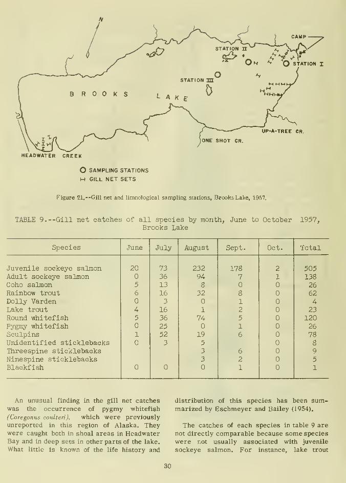
Figure 21. --Gill net and limnological sampling stations, BrcwksLake. 1957.

-Gill net catches of all species by month, June to OctoberBrooks Lake

1957,

Species

Figure 22.—Checking experimental gill net. Brooks Lake, 1957.

and round whitefish (Coregonus cylindraceum) ,

which are usually deep-water species, would

probably have been caught in greater numbers

had more deep sets been made(Rawson, 1951),

Furthermore, fish larger and smaller than

juvenile sockeye salmon were not as likely

to be caught because of mesh selectivity. All

species known to be in the lake were caught in

the gill nets with the exception of north-

em pike (Esoxlucius) and Artie grayling(Thymallus arcticus), which are both rare.

31

The incidental catch of 138 adult sockeye

salmon did not significantly detract from the

production of the 1957 brood year because

most of them were released alive.

Mesh sizes larger than 1 inch were relatively

unproductive except for adult sockeye salmon.

The 3/4-inch size was by far the most efficient

for juvenile sockeye salmon, catching 91 per-

cent of the total catch. Sockeye salmon fry

were not successfully sampled because the

twine on the 1/2-inch size was too thick in

proportion to the interstices.

SEASONAL AND DIURNALCHANGES IN VERTICAL ANDHORIZONTAL DISTRIBUTION

To make valid comparisons of catches it wasnecessary to equate nets of different sizes to

a standard unit. A standard unit was defined

as 75 square feet of mesh; thus each 15-foot-

square panel of type I, II, IV, V, and VII nets

was equal to three units, and each 50-foot

length of Type III and VI nets was equal to

four units (fig. 20).

Even though most catches were made at

night, a 24-hour period was used as the stand-

ard time unit. Nets were checked once each

24-hour period. Thus, a unit of effort was the

catch per 75 square feet of a given mesh size

in a 24-hour period. Catches of species other

than sockeye salmon did not warrant detailed

catch per- unit of effort analysis, nor did

catches of juvenile sockeye salmon, except

for those taken in nets of 3/4-inch mesh.

A comparison of the monthly catch of

sockeye salmon from nets in the littoral area

with the catch from nets in midlake showsthat littoral sets produced a relatively con-

stant catch of about 0.6 sockeye salmon per

75 square feet per day, whereas the midlake

net's catch increased steadily from to 0.65

sockeye salmon per unit per day (table 10).

This indicates that sockeye salmon inhabit

the shallow shoreline areas in the summerand increasingly disperse into deep water as

the season advances. Food studies, as shownlater, further substantiated this conclusion.

Krogius and Krokhin (1956a) found the samegeneral pattern of progressive migration from

littoral to pelagic regions in Lake Dalnee,

Kamchatka, suggesting that this is a universal

behavior trait of juvenile sockeye salmon. If

littoral and midlake nets were sampling the

same population in proportion to its density,

one would expect the catch per hour on littoral

sets to diminish as the catch in midlake nets

increased. This did not occur, and no explana-

tion is offered.

Table 11 shows the depth distribution of

sockeye salmon caught between the surface

and the 45-foot depth at midlake stations for

28 days on which catches were made. FromJuly 21 through August 22, a type V net wasused, simultaneously sampling all depths from

to 45 feet. Fifteen, or 79 percent, of the

sockeye salmon were caught in the surface

net (0-15 feet), while only 4, or 22 percent,

were caught from depths of 15 to 45 feet.

This is in complete agreement with results

from Lake Dalnee, Kamchatka, during the sum-mer months (Krogius and Krokhin, 1948).

From August 29 through October 6 a type I

net was used, permitting sampling only of the

0- to 15-foot level (table 11). When catches

of the surface net of the entire period are

combined, the catch distribution by 5-foot in-

tervals in the upper 15 feet substantiates the

conclusion that juvenile sockeye salmon were

concentrated near the surface to 10 feet,

where 91 percent were caught, while only

9 percent were caught between 10 and 15 feet.

To determine the optimum time of day to

catch fingerlings with the tow net, three gill

nets were checked every 2 hours on August

15 and 16. These consisted of two type II nets

and one type III net, and all were fished in

water less than 15 feet deep. The entire catch

was made between midnight and 4 a.m. Thenight was moonlit and calm, making locating

and checking the nets easy. This night's catch

indicated that best success with tow nets at

the surface in shallow water could be expected

around 2 a.m.

LENGTH AND WEIGHT BYAGE CLASS

It has been previously shown that age

groups of juveniles in Brooks Lake in 1957

32

TABLE 10. --Comparison of monthly littoral and midlake catches of sockeye

salmon in Brooks Lake from June to September 1957 (3/<4-inch mesh only)

lN= number salmon; S= number sets; U= units of 3/1-inch mesh (one unit is 75 squire feet of net)]

TABLE 11.—Number of sockeye salmon caught by depth at stations II and III(midlake) for 28 days with complete data, July 21 to October 6, 1957

Depth (feet)

Date Surface net Middle net Deep net

0-5 5-10 10-15 15-20 20-25 25-30 30-35 35-40 40-45

July

could be distinguished by length-frequency

distributions; therefore, gill net-caught fry

and yearling fish were distinguished on the

basis of size alone without recourse to scale

reading (fig. 19).

The decrease in mean length in June and

July may be explained by the inclusion in June

samples of larger 2-year-olds which sub-

sequently migrated from the lake and were

no longer available in August. Yearlings in-

creased in mean length from 95 mm, in August

to 101 mm. in September. Two-year-olds of

the same age class in the 1957 spring out-

migration (fig. 12) were only 109 mm. long,

or only 8 mm. longer than these fish in the

fall. If it is assumed that yearlings of each

of these year classes grew at the same rate,

the fish we sampled in the fall of 1957 would

gain only an additional 8 mm. during the

ensuing 7 winter months. This projected slow

winter growth contrasts with the 6 mm. of

rapid growth in only 1 month during the

latter part of the summer of 1957.

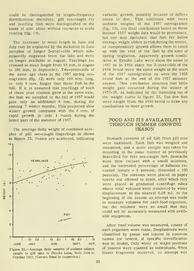
The average daily weight of combined sam-

ples of gill net-caught fingerlings is shown

in figure 23. Points are scattered, indicating

14-1

12-

X

= 6

2-

YEARLINGS

FRY

I

JUNE

10

JULY

20I

10

AUG.

20 I 10 20

SEPT.

I

10

OCT.

Figure 23.— Average daily weights of sockeye salmon

caught in gill nets in Brooks Lake, from June to

October 1957. (Curves fitted by inspection.)

variable growth, possibly because of differ-

ences in diet. This contrasts with moreuniform weights of the 1957 outmigration

(fig. 13). Any final conclusions based on these

limited 1957 weight data would be premature,

but one may speculate that fish far below

average weight either perish during the winter,

or compensatory growth allows them to catch

up with the rest of the fish by the time of

spring migration. Apparently growth condi-

tions in Brooks Lake were about the same in

1957 as in 1956 since the 2-year-olds of the

1954 brood were the same weight at the start

of the 1957 outmigration as were the 1955

brood fish at the end of the 1957 summerseason. This conclusion assumes that little

weight gain occurred during the winter of

1957-58, as indicated by the flattening out of

the weight curve in figure 23. Too few fish

were caught from the 1956 brood to draw any

conclusions on their growth.

FOOD AND ITS AVAILABILITYTHROUGH SUMMER GROWING

SEASON

Stomach contents of all fish from gill nets

were examined. Each fish was weighed and

measured, and a scale sample was taken for

mounting in the same manner as previously

described for fyke net-caught fish. Stomachs

were then excised with a small scissors,

and the estimated percentage of fullness re-

corded (empty = percent, distended = 100

percent). The contents were placed on paper

towels and allowed to drain, after which they

were placed in graduated centrifuge tubes

where total volumes were measured by water

displacement to the nearest 0.05 ml. At the

beginning of the season an attempt was madeto measure volumes for each food organism,

but the volumes were so small that they

could not be accurately measured with avail-

able equipment.

After total volume was measured, counts of

each organism were made. Zooplankters were

classified by genus and insects by commonnames (or orders, if specific identification

was in doubt). Only whole or major portions

of insects were counted as individuals. Wheninsect fragments occurred, no attempt was

35

made to estimate the original number. This

procedure prevented errors of duplication

but made the totals minimal.

Because zooplankters usually were too nu-

merous to count, their numbers were esti-

mated as follows: The bottom of a petri dish

was marked into 1-cm. squares with a dia-

mond-tipped pencil; plankters were uniformly

distributed over the dish; and at least four

squares were counted through a binocular

microscope. The average of the counted

squares was then multiplied by the area of

the petri dish (64 cm. 2) to estimate the total

numbers.

To compare changes in diet, the season

was arbitrarily separated into three periods

(July, August, and September), and food of all

gill net-caught fish from each period wascombined (fig. 24). The following significant

facts are apparent:

1. Contrary to the usual belief that sock-

eye salmon are primarily plankton feeders,

insects were found in an even greater per-

centage of stomachs examined during the

season than was plankton— 30.2 as opposed to

26.2.

2. There was a well-defined progressive

seasonal shift in the diet from insects during

the first part of the summer to plankton during

the latter part of the summer. This sameshift in diet was also found by Russian inves-

tigators at Lake Dalnce, Kamchatka (Krogius

and Krokhin. 1956a).

indicating that availability of insects during

a given year may be more important to the

juveniles' well-being than availability of plank-

ton.

2. Winged insects, which make up the bulk

of the diet, are generally more abundant over

the littoral areas adjacent to land. Thus,

preference (or availability) of insects near

shore during the early summer is conducive

to concentrating sockeye salmon near the

shoreline (table 10).

3. The simultaneous movement to mid-lake areas, decrease in insect feeding, in-

crease in plankton feeding, and increased

incidence of empty stomachs all contribute

to slower growth and early formation of an

annulus.

4. Availability is probably the governing

factor in the lower incidence of insect feeding

as the season progresses. Gross obsers'ations

indicate that the peak of insect production is

in June, coinciding with the period of maximumdaylight. By October very few winged insects

are evident at Brooks Lake.

5. Sockeye salmon select individual food

organisms, even species of plankton. In manyinstances stomachs of fish caught at the sametime and place contained entirely different

organisms. Sometimes a stomach from a

fish would contain only one species of plank-

ton in large numbers, while a fish captured

in adjacent meshes of a gill net would contain

another species.

3. Incidence of empty stomachs increased

progressively through the season.

4. A few sockeye salmon were piscivorous

and even cannibalistic, as indicated in the

"other" category in figure 24. which com-prised mostly fish remains.

Speculation on the implication of these facts

leads to some interesting tentative conclu-

sions;

1. The period of insect feeding corre-sponds to the period of most rapid growtii of

juveniles during the spring and early summer.

The shift from insects to plankton through

the season in terms of total numbers is shownin table 12. Total numbers of organisms are

shown rather than frequency of occurrence as

in figure 24, The overall ratio of individual

Insects to plankton organisms was 1:25. Thepercentage fullness of stomachs through the

season was also measured (fig. 25). Sockeye

salmon ate less as the season progressed, with

the Incidence of to 10 percent fullness morethan doubling, from 22 percent In June and

July to 59 percent In September. This slacken-

ing of feeding further explains the late summerdecrease In growth rate and fall annulus

forniatlon.

36

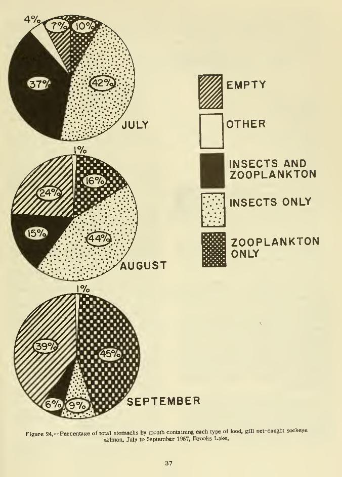
JULY

AUGUST

EMPTY

OTHER

• * <

INSECTS ANDZOOPLANKTON

INSECTS ONLY

ZOOPLANKTONONLY

SEPTEMBER

Figure 24.-- Percentage of total stomachs by month containing each type of food, gill net-caught sockeye

salmon, July to September 1957, Brooks Lake.

37

TABLE 12.—Frequency of occurrence of insects and plankton in sockeye salmoncaptured in Brooks Lake, June 27 to September 12, 1957

, . . Total Total Plaiikters Insectscontaining

—

T———7—plankters insects per fish per fishPeriod

Plankton

June 27-July 31August 1-31September 1-12

Total

Number

496A

89

202

Number Number Number Number Number

83 45,042 1,850 919 22120 36,576 5,202 572 4327 101,289 314 1,U8 11

230 182,907 7,366 905 32

0-IO% r~l II -50%^^ 51-100%!

JUNE 27- JULY 31

AUGUST 1-31

SEPTEMBER 1-12

Iri

''

i

'

irVi'i i i ;• ••'

.

• ' •••i'i i'

25 50 75

PERCENT100

Figure 25,-- Percent fullness of stomachs from gill

net-caught juvenile sockeye salmon. Brooks Lake,

June 27 to September 12, 1957,

The species composition of food items wasalso compared through the season (table 13).

Four species of zooplankton ( Daphnia longispina,

Bosmina longirostrls, Bosmina coregoni, andCyclops sp,) made up over 96 percent of the

plankton. The relative percentages of each

species were almost identical in July and

September, whereas in August, Cyclops doubled

in frequency of occurrence and Daphnia oc-

curred only one-third as often. During this time

no major fluctuations in actual abundance of

plankton occurred in the lake, as shown in

part IV, the section on plankton distribution

and abundance.

More than 76 percent of the insects eaten

by juvenile salmon were midges. This high

ratio of midges to other insects in stomachswas quite constant through the summer in

contrast to marked differences In the speciescomposition of plankton in the diet from

month to month. The abundance and avail-

ability of midges is apparently an important

factor in sockeye salmon ecology at BrooksLake,

The absolute number of each kind of or-

ganism in stomachs probably is of little

significance, except as a relative measureof the number of separate ingestions or food

selections made. Ninety-six percent of in-

dividual organisms were plankters, and only

4 percent were insects (table 13).

Sockeye salmon juveniles fed upon a greater

variety of food than any other fish species

present in Brooks Lake (table 14). This food

included 9 different planktonic forms (10

including copepod nauplii), 19 insects, and 3

identified fish (sockeye salmon, sculpins, and

pygmy whitefish). Two other fish species in

Brooks Lake (whitefish and sticklebacks) are

competitors for plankton food. This competi-

tion was probably of little consequence in

1957, considering the high density of zoo-

plankton and low density of sockeye salmon,

whitefish, and sticklebacks. In years of greater

densities of juvenile sockeye salmon, however,

competition from sticklebacks might be a

serious problem. Krogius and Krokhin (1956a,

1956b) and Krogius (1951) found in LakeDalnee, Kamchatka, that survival of sockeye

salmon is directly related to the abundance

of threespine sticklebacks.

All fish except blackfish were insectivorous,

and competition for winged insects may have

38

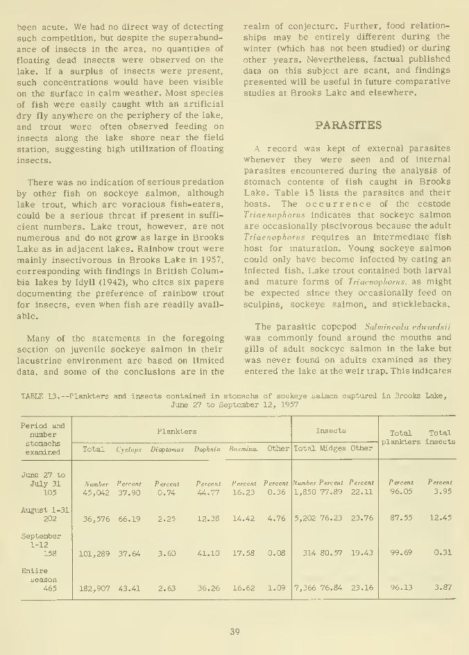
been acute. We had no direct way of detecting

such competition, but despite the superabund-

ance of insects in the area, no quantities of

floating dead insects were observed on the

lake. If a surplus of insects were present,

such concentrations would have been visible

on the surface in calm weather. Most species

of fish were easily caught with an artificial

dry fly anywhere on the periphery of the lake,

and trout were often observed feeding on

insects along the lake shore near the field

station, suggesting high utilization of floating

insects.

There was no indication of serious predation

by other fish on sockeye salmon, although

lake trout, which are voracious fish-eaters,

could be a serious threat if present in suffi-

cient numbers. Lake trout, however, are not

numerous and do not grow as large in Brooks

Lake as in adjacent lakes. Rainbow trout weremainly insectivorous in Brooks Lake in 1957,

corresponding with findings in British Colum-bia lakes by Idyll (1942), who cites six papers

documenting the preference of rainbow trout

for insects, even when fish are readily avail-

able.

Many of the statements in the foregoing

section on juvenile sockeye salmon in their

lacustrine environment are based on limited

data, and some of the conclusions are in the

realm of conjecture. Further, food relation-

ships may be entirely different during the

winter (which has not been studied) or during

other years. Nevertheless, factual published

data on this subject are scant, and findings

presented will be useful in future comparative

studies at Brooks Lake and elsewhere.

PARASITES

A record was kept of external parasites

whenever they were seen and of internal

parasites encountered during the analysis of

stomach contents of fish caught in BrooksLake. Table 15 lists the parasites and their

hosts. The occurrence of the cestode

Triaenophorus indicates that sockeye salmon

are occasionally piscivorous because the adult

Triaenophorus requires an intermediate fish

host for maturation. Young sockeye salmon

could only have become infected by eating an

infected fish. Lake trout contained both larval

and mature forms of Triaenophorus, as might

be expected since they occasionally feed on

sculpins, sockeye salmon, and sticklebacks.

The parasitic copepod Salmincola eduardsii

was commonly found around the mouths and

gills of adult sockeye salmon in the lake but

was never found on adults examined as they

entered the lake attheweir trap. This indicates

TABLE 13.—Plaakrters and insects contained in stomachs of sockeye salmon captured in Brooks Lake,

June 27 to September 12, 1957

Period andnumber

TABLE 14. --Checklist of organisms found in stomachs of fish caught by gill nets, beach seines, and tow nets.Brooks Lake, 1957

Juvenile„ , Coho Rainbow Dolly Lake Round Pygmy _ , . Stickle- Black-Organisms sockeye , ,, , ,.,.,, . ,. , Sculpins , , ,. ,

, salmon trout Varden trout whitefish whitefish backs fishsalmon

ZooplanktonBosmina curegoni X x xBosmina longiTostris x x xCeriodaphnia xChydorus x XConochilus xCyclops sp. X XXXOaphnia longispina x x x ic

Diaptomus x xEurycercus XHolopedium gibberum x xCopepod nauplii x

Plecoptera (Stoneflies) x x xOdonataDamselflieB xDragonflies xDragonfly naiads x x

ColeopteraBeetles x x

HemipteraBack swimmerB x xWaterboatmen xWaterstriders xFragments x x x x

HomopteraLeafhoppers x xFragments x x x

NeuropteraLacewings x x x

Trichoptera(Caddisfl.ies) x x x x x x xLepidopteraMoths X

DipteraCrane flies x xDeer flies xHorn flies xHorse flies x xMidges (larvae) x x x x x x xMidges (winged) x x x x x x xMosquitoes xFragments x x x x x

HymenopteraAnts (winged) x x xBees XWasps XXX X

Amphipods x xClams X XLeeches ^Mites XSnails XXXSpiders x xPygmy whitefish x xSalmon eggs

Salmonids x x x xSculpins X XSticklebacks x x

^

40

TABLE 15.—Parasites and their hosts found in catches of fish from Brooks Lake, 1957

Name and type

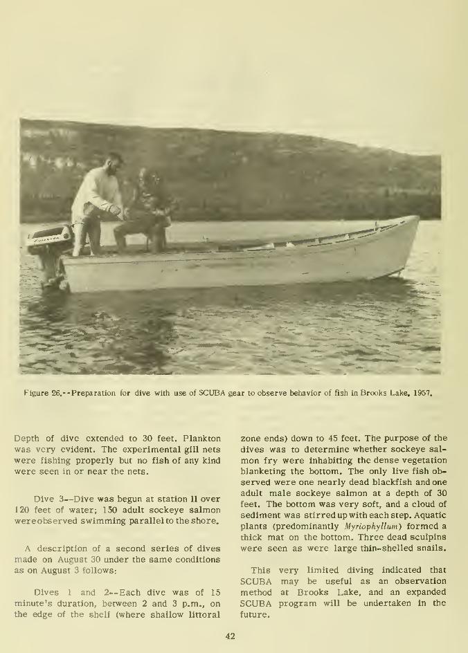
Figure 26.- -Preparation for dive with use of SCUBA gear to observe behavior of fish in Brooks Lake, 1957.

Depth of dive extended to 30 feet. Plankton

was very evident. The experimental gill nets

were fishing properly but no fish of any kind

were seen in or near the nets.

Dive 3—Dive was begun at station II over

120 feet of water; 150 adult sockeye salmonwereobserved swimming parallel to the shore.

A description of a second series of dives

made on August 30 under the same conditions

as on August 3 follows:

Dives 1 and 2—Each dive was of 15

minute's duration, between 2 and 3 p.m., on

the edge of the shelf (where shallow littoral

zone ends) down to 45 feet. The purpose of the

dives was to determine whether sockeye sal-

mon fry were inhabiting the dense vegetation

blanketing the bottom. The only live fish ob-

served were one nearly dead blackfish and one

adult male sockeye salmon at a depth of 30

feet. The bottom was very soft, and a cloud of

sediment was stirred up with each step. Aquatic

plants (predominantly Myriophyllum) formed a

thick mat on the bottom. Three dead sculpins

were seen as were large thin- shelled snails.

This very limited diving indicated that

SCUBA may be useful as an observation

method at Brooks Lake, and an expanded

SCUBA program will be undertaken in the

future.

42

PART IV. LIMNOLOGY AND ITS RELATION TO SOCKEYE SALMON

Limnological data were collected in 1957

concurrently with studies of the biology of

sockeye salmon discussed in Parts I, 11, and

111. One form of Liebig's Law, or the Law of

the Minimum, states that productivity is lim-

ited by the nutrient present in the least

amount at any given time. If one essential

element is in short supply, regardless of the

abundance of other essential elements, pro-

duction may be limited. Part IV describes the

limnology of the lake and stream environments

and the significance of selected key factors,

including nutrients, in the biology of sockeye

salmon (fig. 27).

The objectives of the studies were to:

(1) Measure relative seasonal abundance of

zooplankton and phytoplankton at three repre-

sentative stations and relate to the distribu-

tion and the diet of juvenile sockeye salmon;

(2) determine the bottom morphometry of

Brooks Lake by surveys with a recording echo

sounder; (3) determine the relative abundance

of bottom fauna and through food studies,

relate to utilization by sockeye salmon; (4) de-

termine the following qualities that influence

productivity by analyzing lake water at 2-week

intervals at representative midlake stations

—

temperature, phosphorus, nitrogen, silica, tur-

bidity, transparency, oxygen, hydrogen ion

concentration, and alkalinity and total hard-

ness; (5) determine the primary productivity

of Brooks Lake by the carbon^ ^ method;

(6) record continuously the temperature of

the gravel water of Brooks River and OneShot Creek; (7) record fluctuations in lake

level; and (8) record climatological data and

solar radiation.

TURBIDITY

TRANSPARENCY

FISH (tockty* •olmon)

ZOOPLANKTON - INSECTS

PHYTOPLANKTON (dlotont)

TEMPERATURE

OXYSEN

pH

ALKALINITY PHOSPHORUS NITROSEN SILICA TOTAL HARDNESS

Figure 27,-- Probable relation of sockeye salmon pro-

duction and chemical and physical water qualities in

Brooks Lake.

PLANKTON AND ITS RELATION TOJUVENILE SOCKEYE SALMON

Information was needed on the kinds and

abundance of zooplankton in Brooks Lake be-

cause, as previously discussed in Part III in

the section on food of juvenile sockeye salmon,

it is an important food item. Phytoplankton

are not usually eaten by juveniles, but infor-

mation on kinds and abundance gives useful

clues to basic productivity and to limiting

chemical constituents of the water.

Beginning June 27, when weather permitted,

plankton collections were made at 10-day in-

tervals at three stations (fig. 21). Zooplankton

was collected with a Clarke- Bumpus sampler

with a number 10 net, and phytoplankton wascollected with a 3-liter Kemmerer water

sampler.

Station I was located on the edge of the

littoral area in 5 m. of water; station II,

southwest of station I in 35 m.; and station III,

in midlake southwest of station II in 67 m.

Depths sampled were as follows: station I,

surface and 5 m.; station II, surface, 5, 10,

and 25 m.; station III, surface, 5, 10, 25, 35,

and 50 m. All tows were made between 10 a.m.

and 1 p.m.

Zooplankton

The Clarke- Bumpus sampler was an open,

nonclosing type and was operated according

to recommendations of the inventors (Clarke

and Bumpus, 1950). To ensure that the mouth

of the instrument remained perpendicular to

the flow during horizontal tows and to prevent

water from entering the net while it was being

raised or lowered to the desired sampling

depth, a 20-pound weight was fastened to the

lower edge of the sampler frame.

After each haul the net and bucket were

rinsed with lake water and the contents drained

into a small screw-top jar containing a solu-

tion of 3 percent formalin. Plankters were then

transferred to an alcohol solution for storage

until counts and identifications could be made.

Identifications were made from keys by Pennak

(1953). Numbers of plankters were estimated

43

as follows: The volume of preserved concen-

trate was measured with a graduated cylinder,

and the number of each organism determined

by the formula

cv

n =

in which n = number of plankters per liter of

original water; c = number of plankters in

1-ml. cell; v = volume of concentrate in milli-

liters; and 1 = volume of original water sam-pled in liters. For example, if the samplerrecorded 75 revolutions (1 revolution = 4

liters), the sample measured 100 ml., and the

count was 60 plankters in a 1-ml. Sedgwick-

Rafter cell, the calculated number of organisms

per liter of lake water would be

n = 60 X 100

300

n= 20 organisms per liter.

Counts were made by filling a 1-ml. Sedg-

wick-Rafter cell with thoroughly mixed con-

centrate. Guidelines were scored on the under-

side of the cell with a diamond- tipped pencil

to help prevent duplication of counts. Total

numbers of each species in the cell werecounted. Initially, duplicate samples of con-

centrate were counted to check the technique

and develop skill in counting. Since counts of

organisms in duplicate samples were found

to be consistent, counts were later made only

on single samples of concentrate.

The following six genera and species of zoo-

plankters were collected: Daphnia longispina,

Bosmina longirostris, Bosmina coregoni, Holopedium

gihherum, Cyclops sp., and Diaptomus sp. Spe-

cies identification of Cyclops and Diaptomus,

could not be made with the microscopes avail-

able at the field station. Eurycercus was found

in stomachs of round whitefish but never in

plankton collections, and the rotifer Conochilus

was found once in a sockeye salmon stomach;therefore, the two zooplankters were presentin the lake in 1957 but were not abundant.

An unidentified cladoceran was found in

stomachs and plankton collected between water

depths of 5 and 25 meters at stations II and III.

Samples of live and preserved individuals of

this species were sent to D. K. Milliard of the

Arctic Health Research Center at Anchorage,

Alaska, but he was unable to identify them.

At Hilliard's suggestion, samples were sent

for identification to Kaj Berg, FreshwaterBiology Laboratory, University of Copenhagen,

Copenhagen, Denmark. Berg and a colleague,

Mr. Ren, identified it as an arctic form of

Holopedium gibberum. An excerpt from Berg's

letter follows: "The Cladoceran in question

belongs to the species Holopedium gibberum

Zaddach. However, they do deviate from the

typical form of the species as the gelatinous

case is considerably lower and the abdomensomewhat slimmer than on this species. It is

a hunger form or what the Germans call

'Kummer form.' But these differences are

not enough to establish a variety or subspecies

on the existing material, as there is an even

transition from the typical form to the one

present, which is of Arctic origin. It turns on

a form, which—owing to the short period of

activity in the Arctic fresh waters—mustcarry out its development and reproduction

in the shortest time possible and with a mini-

mum of use of material on account of the low

content of food in the Arctic lakes. From a

biological point of view the animal can fur-

thermore do without the big gelatinous case

in the fairly cold water, as the viscosity here

is great. We know analogous forms of the spe-

cies from Greenland."

The average numbers of zooplankters per

liter of water sampled for each of the three

stations were significantly different (fig. 28).

Oi—27

JUNE14

JULY24 13

AUG.

23 3

SEPT.

Figure 28.— Numbers of zooplankters per liter ot lake

water, averages of all depths for each sampling date,

June 27 to Sept. 3, 1957, Brooks Lake.

44

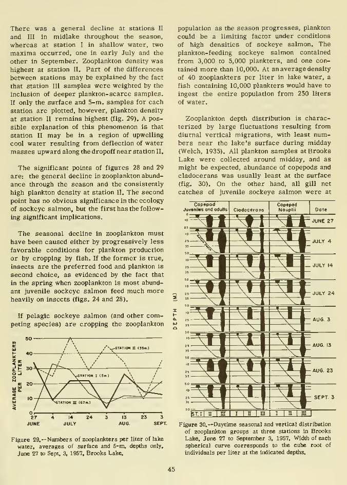
There was a general decline at stations II

and III in midlake throughout the season,

whereas at station I in shallow water, two

maxima occurred, one in early July and the

other in September. Zooplankton density was

highest at station II. Part of the differences

between stations may be explained by the fact

that station III samples were weighted by the

inclusion of deeper plankton- scarce samples.

If only the surface and 5-m. samples for each

station are plotted, however, plankton density

at station II remains highest (fig. 29). A pos-

sible explanation of this phenomenon is that

station II may be in a region of upwelling

cool water resulting from deflection of water

masses upward along the dropoff near station II.

The significant points of figures 28 and 29

are: the general decline in zooplankton abund-

ance through the season and the consistently

high plankton density at station II. The second

point has no obvious significance in the ecology

of sockeye salmon, but the first has the follow-

ing significant implications.

The seasonal decline in zooplankton musthave been caused either by progressively less

favorable conditions for plankton production

or by cropping by fish. If the former is true,

insects are the preferred food and plankton is

second choice, as evidenced by the fact that

in the spring when zooplankton is most abund-

ant juvenile sockeye salmon feed much moreheavily on insects (figs. 24 and 28).

If pelagic sockeye salmon (and other com-peting species) are cropping the zooplankton

Oi-27 4 14 24 3 13 23 3

JUNE JULY AUG. SEPT.

Figure 29.— Numbers of zooplankters per liter of lake

water, averages of surface and 5-m. depths only,

June 27 to Sept. 3. 1957, Brooks Lake.

population as the season progresses, plankton

could be a limiting factor under conditions

of high densities of sockeye salmon. The

plankton-feeding sockeye salmon contained

from 3,000 to 5,000 plankters, and one con-

tained more than 10,000. At an average density

of 40 zooplankters per liter in lake water, a

fish containing 10,000 plankters would have to

ingest the entire population from 250 liters

of water.

Zooplankton depth distribution is charac-

terized by large fluctuations resulting fromdiurnal vertical migrations, with least num-bers near the lake's surface during midday(Welch, 1935). All plankton samples at Brooks

Lake were collected around midday, and as

might be expected, abundance of copepods and

cladocerans was usually least at the surface

(fig. 30). On the other hand, all gill net

catches of juvenile sockeye salmon were at

a.

UJ

Figure 30.—Daytime seasonal and vertical distribution

of zooplankton groups at three stations in Brooks

Lake, June 27 to September 3, 1957. Width of each

spherical curve corresponds to the cube root of

individuals per liter at the indicated depths.

45

night. They were mostly captured near the

surface (table 10) where they fed on plankton,

especially in late summer (fig. 24). Presum-ably sockeye salmon juveniles were attracted

to the surface waters by the nighttime con-

centration of plankton. Because our plankton

samples were taken in the day and our fish

samples at night, it is not surprising that the

depths of maximum density of sockeye salmon

and zooplankton did not coincide. It would be

enlightening to obtain a series of day and

night plankton samples at Brooks Lake to

compare abundance at different depths through

a series of 24-hour periods but we were unable

to undertake this in 1957.

On the eight sampling dates weather ranged

from clear and calm to rough and windy.

There was no discernible relation of weather

conditions and horizontal or vertical plankton

distribution. This is not surprising since the

maximum concentrations occurred at depths

of 5 m. and more, below the influence of

surface water conditions.

Of zooplankters eaten by sockeye salmon,

46 percent were the copepods, Cyclops and

Diapinmus, and 54 percent were thecladocerans, Daphnia and liosmina. This im-plies that plankton-feeding sockeye salmondefinitely prefer cladocerans to copepods,

because copepods were invariably moreabundant than cladocerans in samples (fig. 30).

Salmon seldom ate copepod nauplii, and there-

fore the significance of their distribution and

abundance to sockeye salmon is only indirect

in ultimate abundance of copepods.

Figure 30 requires some explanation and

interpretation. The black shapes are spherical

curves (Birge and Juday, 1922). They repre-

sent three-dimensional columns of relative

plankton densities in a vertical water column

at each of the three stations. The water column

at each station was sampled at each indicated

depth. The bottom depth was 5 m. at station I;

35 m. at II; and 67 at III.

The significant points in figure 30 are:

I. Samples at station I are not repre-

sentative of the main body of the lake. Exceptfor copepod nauplii on July 4 and 14, zoo-

plankters were less dense at station I than at

II and III.

2. Zooplankters were usually less abund-

ant in the surface 5 m. of water at midday

than at lower depths, probably because of the

inhibiting effect of light. Usually the region of

highest concentrations was from 5 to 10 m.

3. Plankton density was greatest during

the early summer and decreased gradually

through the summer and fall.

4. Copepod juveniles and adults werealways more abundant than cladocerans or

copepod nauplii.

5. Relative vertical distribution showedlittle stratification, indicating that the lake

contained zooplankton throughout the season at

all depths.

From 1926 to 1930, limnological studies

were conducted at Karluk Lake on Kodiak

Island (Juday, Rich, Kemmerer, and Mann,

1932). Karluk Lake was then a major pro-

ducer of sockeye salmon; conditions for sock-

eye salmon production were presumably satis-

factory. Since Karluk and Brooks Lakes are

in the same general geographic area and are

approximately the same size, general com-parisons should be useful and valid, liosmina,

Daphnia, Cyclops, and Diaplomns were the

dominant forms in both lakes. Maximum abund-

ance of Daphnia was considerably greater in

Brooks Lake: 21 per liter compared with 9

per liter in Karluk Lake. The largest catch of

liosmina in Karluk Lake was 13 per liter

compared with 11 in Brooks Lake. Maximumabundance of Diaptomns in Karluk Lake was22 per liter compared with 53 per liter in

Brooks Lake, and for Cyclops, it was 145 per

liter compared with 31 in Brooks Lake. Forcopepod nauplii, maximum abundance in Karluk

Lake was 100 per liter; in Brooks Lake it

was 56. The one striking difference between

Brooks and Karluk Lakes is that at Karluk

Lake rotifers reportedly were the most abund-

ant form of all zooplankters, while at Brooks

Lake rotifers were scarce and were never

found in net or centrifuge samples (they were

found in stomach samples).

46

Further comparisons could be made, but it

is clear that the zooplankton of Brooks and

Karluk Lakes are generally similar. It is

not known whether the abundant rotifers in

Karluk Lake were utilized by sockeye salmon.

In conclusion, there is no evidence of a de-

ficiency in numbers of genera or actual abund-

ance of zooplankters utilized by Brooks Lake

sockeye salmon in 1957.

Zooplankton probably do not limit sockeye

salmon production at Brooks Lake where

fish densities are low. Even the lowest plankton

densities measured were relatively high and

were similar to densities in Karluk Lake

during its period of high sockeye salmon

production (Juday, Rich Kemmerer, and Mann,

1932).

Phytoplankton

To measure the relative abundance of phyto-

plankton and protozoa, samples were taken at

the same sampling times and locations as for

zooplankton, as described on page 43. Only

2 liters of each 3-liter sample were used to

measure phytoplankton abundance, the third

liter being utilized for chemical analyses.

Samples were transported to the lakeside

laboratory as quickly as possible, and the

entire 2 liters was immediately centrifuged

in a high-speed plankton centrifuge. The vol-

ume of plankton for each sample was deter-

mined by transferring the concentrate from the

metal centrifuge cup into a small graduated

glass centrifuge tube and recentrifuging in a

geared hand-operated centrifuge. After the

volume was determined, a measured quantity

of 3 percent formalin was added to preserve

the sample for later counting and identification.

Counts were made with a large-aperture

pipette by placing 1 ml. of the concentrate into

a Sedgwick-Rafter cell and counting randomfields until a minimum of 100 individual plank-

ters (or colonies In multicellular species)

were counted. Many green algae and protozoa

were fractured during the centrlfuglng.

Hiitryi)r.ori:us colonles in particular were evi-

dent in uncentrifuged samples but were rarely

seen afterward.

The underside of the Sedgwick-Rafter cell

was marked with a diamond-tipped pencil to

partition the sample into sections as an aid in

preventing counting fields more than once.

Counts were converted to plankters per

liter with this formula:

n = KJCv

1

in which n^ = number of plankters per liter of

original water, K = a constant, x = average

count per field, v = volume of original pre-

served concentrate, and 1 - volume of original

water sample (in liters).

The constant (K) was the number of fields

of view in the entire cell. It was calculated

by first measuring in millimeters the diameter

of a field of view under the microscope and

then calculating the area of the circular field

of view. The area of the entire cell (1,000

square mm.) was then divided by the area of

a single field; the resulting quotient was K.

The average count per field (x) was the

quotient resulting from dividing the total count

(about 100) of each plankter by the number of

fields of view examined.

This procedure produced a relative measureof seasonal and depth distributions of phyto-

plankton and protozoa but was only an ap-

proximation of actual numbers per original

liter of lake water. Only recognizable frag-

ments or cells were counted, which tended

to minimize counts; on the other hand, counts

were increased by regarding as individuals

each fragment of colonial phytoplankton broken

apart during centrlfuglng. The numbers per

liter of each of the three most abundant

phytoplankton groups (green algae, blue-green

algae, and diatoms) and protozoa were plotted

In the same way as were zooplankton (fig. 31).

A checklist wascompiledof all genera of phyto-

plankton and protozoa encountered (table 16).

Phytoplankton and protozoan distributions,

both vertically and in relative seasonal abund-

ance, were much more variable than zoo-

plankton (figs. 30 and 31). Since diatoms wereabundant at all depths throughout the season,

zooplankters had sufficient diatoms for food.

47

0.UJo

Figure 31.--Seasonal and vertical distribution ofphyto-

plankton and protozoan groups at three stations in

Brooks Lake from June 27 to September 3, 1957,

Width of each spherical curve corresponds to the

cube root of individuals per liter at the indicated

depths. Dot indicates absence of representatives of

a group in that sample.

Green algae showed two pulses in abundance,

the larger in late June and early July and the

smaller in early August. Maximum density of

the June pulse of green algae was 147,000

individuals per liter at station I and wascoincident with a dense bloom of green algae

on the littoral zone.

Blue-green algae (two genera. Microcystis

and Lyngbya) also showed two pulses, one on

July 4 and the other in mid-August. This abund-

ance of blue-green algae is interesting because

oligotrophic lakes such as Brooks are usually

deficient in blue-green algae (Rawson, 1956).

Maximum density of blue-green algae was57,000 individuals per liter at the 50-meterdepth at station III on August 23.

On the basis of phytoplankton population.

Brooks Lake does not entirely fit the tradi-

tional oligotrophic classification. Throughoutthe summer, diatoms were the dominant form,

and Melosira was usually the dominant genus.

Melosira is usually regarded as an indicator of

eutrophy rather than oligotrophy, but at Brooksand Great Slave Lakes Melosira was the domi-nant diatom. Other eutrophic indicators werealso found, namely, Synedra, Fragillaria, and

Asterionella. Maximum density of diatoms

was 181,000 per liter at station 1 on June 27.

Possibly an even greater density occurred

in the spring before sampling began.

TABLE 16. -Genera of plankton fovind in water samples fromBrooks Lake, 1957

Green algae Blue-green algae Diatoms Protozoa

AnkistTodesmus

Botryococcus

Closterium

PediastTum

Phacotus

PleuTococcus

Scenedesmus

Spirogyra

StaurastTum

Lyngbya

Microcystis

Asterionella

Cyclotella

Cymhella

Diatoma

Fragillaria

Gomyhonema

Melosira

Navicula

Stephanodiscus

Synedra

Tabellaria

Ceratium

Dinobryon

Vorticella

48

Protozoa formed a small and variable por-

tion of the total plankton, reaching maximumabundance of 17,000 individuals per liter on

August 23 at the 5-meter depth at station 11.

The total plankton of Brooks Lake in 1957

was generally abundant throughout the season

and well distributed to all depths.

MORPHOMETRY

The bottom morphometry of Brooks Lake

had to be determined before we could makea map on which we could base planning of

future biological and chemical sampling pro-

grams. A Raytheon portable recording echo

sounder model DE 119B, which could be read

to within half a foot over a range of to 245

feet, was used, A hand-sounding line was used

to calibrate the sounder and to sound the areas

beyond maximum range of the instrument.

A bracket consisting of a 1/4-inch bolt

through the left gunwale, with the outer end

embedded in a small wooden fairing block,

was used to mount the transducer rod on the

boat. The transducer rod was clamped to the

outside of this block so that it pivoted on this

point (fig. 32). The upper projecting end of the

transducer rod was guyed in place by two

stout lengths of twine secured to the gunwale

fore and aft. When not in use the transducer

rod was pivoted so that its axis lay along the

gunwale.

Sounding techniques and construction of the

map followed the methods described by Warner(1953). Fifty-seven sounding transects weremade across Brooks Lake (fig. 33). Based on

these transects, a large-scale master map wasdrawn with contour intervals of 10 feet, which

are increased to 40-foot intervals in figure

34 for clarity.

The surface area of the lake is 28.9

square miles, excluding the islands. Maximumlength is 10.7 miles and maximum width, 4.1

miles. Mean width is 2.7 miles. Maximumdepth is 258 feet at the point indicated on

figure 34, and mean depth is 148 feet. Length

of shoreline is 31.5 miles and shoreline

development, 1.7. The volume is 2,745,600

acre feet. The surface altitude is 62 feet

above sea level.

BOTTOM FAUNA

A limited number of samples were taken

with an Ekman dredge at stations I, II, and 111

(fig. 21) to learn the general composition and

distribution of bottom fauna. In general, bottom

fauna (mainly Diptera larvae) was abundant

at station I (5 m.) but decreased to almost

none at station III (67 m.). Our studies of

sockeye salmon food indicate that bottom fauna

is not directly important to sockeye salmon.

This finding agrees with the Cultus Lakestudies of Ricker (1952).

WATER QUALITY

Temperatures and chemical qualities of

Brooks Lake water were determined at sta-

tions I, II, and III, which were selected as

representative of the shallow-, medium-, and

maximum-depth areas of the lake. Samples

at each station were taken at 10-day intervals

between July 4 and September 3. The water

qualities chosen for measurement were those

believed to be most likely to be limiting

factors or to affect production of sockeye

salmon. Samples were collected with a 3-liter

Kemmerer water sampler, transferred im-

mediately to brown, ground-glass stoppered

bottles and were analyzed within 30 hours.

Samples kept overnight before being analyzed

were kept cool by storing in a refrigerator.

Glassware was scrupulously cleaned with de-

tergent and rinsed with distilled water imme-diately before use.

To insure use of identical techniques for

comparative purposes in future years, a de-

tailed description of each analytical technique

was prepared. Pertinent data were recorded

at the time a sample was taken.

Temperatvire

Water temperature is of vital importance

to the entire biota of a lake and is one of the

principal factors in determining overall pro-

duction.

49

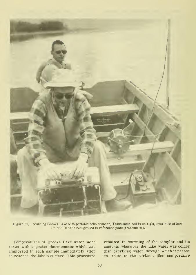
Figure 32,--Sounding Brooks Lake with portable echo sounder. Transducer rod is on right, over side of boat.

Point of land in background is reference point (transect 41).

Temperatures of Brooks Lake water were resulted in warming of the sampler and Its

taken with a pocket thermometer which was contents whenever the lake water was colder

immersed in each sample immediately after than overlying water through which it passed

it reached the lake's surface. This procedure en route to the surface. (See comparative

50

BROOKSRIVER

UP-A-TREE CR.

ONE SHOT CR.

HEADWATER

CREEK

Figure 33.--Sounding transects of Brooks Lake made in 1957 with portable echo sounder.

CONTOUR INTERVAL 40 FEET

Figure 34.--Bottom contour map of Brooks Lake.

readings October 3 in figure 35.) For this

reason, actual temperatures at deeper points

were slightly lower than indicated.

Figure 35 shows the temperature profiles

at each station for successive dates of sam-pling. Because temperatures were recorded

only for selected depths, and no continuous

temperature profiles were obtained, little was

learned on presence of or characteristics of

the thermocline. The range of temperatures

from surface to bottom was quite small,

indicating that thermal stratification was not

pronounced; the maximum range was 17° F.in

65 m. on August 23.

From July 24 through August 23, surface

temperatures at station II were less than at I

51

JULY JULY JULY AUG AUG. AUG. SEPT SEPT OCT.4 I 14 I 24l 3 I 13 I 23 I 3 |I3.23| 3

Station I

„t,. ,...U,.*^,U ,../ ..l„.. .. .t . |.. . ...u.^.t.. .^, ..ai^. ,-,l , . . ..,M4.. . ...H^g

fPOCKETStation n ^

" iShr 5'

.: ri/

l/

l/ l/V

•.fmmrmijjii.. •iMm.T'v'Mt-ir^wOoiJOM

a 10

Station HI

30 60 50 60 50 60 SO 60 50 60 50 60 50 60 50 60 SO 60

TEMPERATURE C F.)

Figure 35.— Brooks Lake vertical temperatures, sta-

tions I, II. and III, July to October 1957.

or III. This corresponds with greater zoo-

plankton densities at station II over those of I

and III (figs. 28 and 29). It is conjectured

that station II Is in a region of upwelllng of

cold water masses originating from the depths.

From the bottom configuration, as indicated

by the contour map (fig. 34), and from the

action of submerged gill nets at station II,

such upwelling is likely when strong winds

sweep the lake. Further study is needed to

learn the reasons for the measured differences

between stations II and III.

Phosphorus

Soluble phosphorus was measured with a

Klett-Summerson photoelectric colorimeter

as described by P. R. Nelson. * Great carewas required in analysis because of micro-quantities present and the danger of contamina-tion.

Phosphorus and nitrogen (together with car-

bon and hydrogen) are the principal consti-

tuents of living cells and are usually present

in extremely small quantities in lake waters.

It is likely that if a nutrient deficiency werepresent, one of these would be in short supply.

Compilation of field methods for water analysis.

1952. [Unpublished typewritten report.] On fileatBCF

Biological Laboratory, Auke Bay, Alaska.

The range of phosphorus was from to

0.0152 p.p.m., and amounts were quite uniform

at all depths and dates (table 17). These data

indicate that when relatively few spawnersare present, as was the case in 1957, car-

casses of spawners do not contribute a meas-urable amount of phosphorus to the lake. Onthe contrary, phosphorus declined slightly

through the season, with the least amountson September 3. This conclusion was also

reached in Cultus Lake studies by Ricker

(1937).

Organic bottom sediments probably play a

more important part in supplying available

phosphorus than do salmon carcasses. Ourquantitative phytoplankton sampling indicates

that the biomass of the standing crop of

phytoplankton must be much greater than that

of salmon carcasses at any one time, and over

a period of a year it must be vastly greater.

It is probable that renewal of the supply of

phosphorus is not dependent on salmon car-

casses in a large lake such as Brooks, with

relatively abundant plankton and small salmonruns.

Since phosphorus is present throughout the

season, it is probably not a limiting factor on

plankton production. Phosphorus is one of the

principal living cell constituents and is taken

up and readily stored by phytoplankton (Ruttner,

1953). If it were a limiting factor, measure-ments would be zero because phytoplankton

would utilize all of it as soon as it appeared.

Thus, if it is present in detectable quantities,

it may be regarded as being in adequate sup-

ply.

Nitrogen

Nitrite nitrogen was measured with a Klett-

Summerson photoelectric colorimeter accord-ing to directions in Nelson's compilation. * Aswith phosphorus, great care was required in

the analysis.

Nitrite ranged from to 0.0050 p.p.m. and

was relatively uniform in quantity and vertical

5 See footnote 4.

52

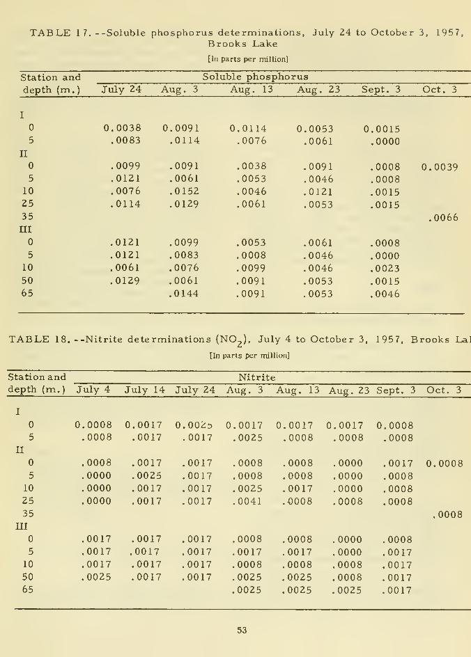
TABLE 17. --Soluble phosphorus determinations, July 24 to October 3, 1957,Brooks Lake

[In parts per million]

Station and

distribution through the summer (table 18).

Nitrite was detected at each station on every

sampling date, although it was not found at

certain depths on July 4 and August 23. Thezero measurements may not be absolute be-

cause 0.0008 p.p.m. was the smallest quantity

our equipment could detect. Quantities be-

tween absolute and 0.0008 were recorded

as zero.

The absence of an increase of nitrite in the

autumn indicates that decaying salmon car-

casses are not important in increasing de-

tectable nitrogen supplies in the lake, at

least when relatively small numbers of sal-

mon are present, as they were in 1957. If

appreciable nitrogen had been added, its ef-

fects should have been apparent on the August

23 and September 3 sampling dates. Further-

more, the prime source of nitrogen in lakes

is probably from the atmosphere rather than

through organisms (Ruttner, 1953).

Silica

Silica determinations (table 19) were madewith a Klett-Summerson photoelectric colori-

meter. Silica is the major constituent of the

skeletal structure of diatoms, which are usu-

ally the principal phytoplankton food for zoo-

plankton in oligotrophic lakes. A majordecrease in silica often occurs after a

bloom of diatoms (Ruttner, 19 53), so a

shortage of silica could limit diatom produc-

tion.

Silica ranged from a low of 9.4 to a high

of 12.0 p.p.m. Si02 and was relatively uniform

throughout the season and at all water depths.

This is consistent with the uniform distribu-

tion and abundance of diatoms, which are the

main cause of variations in silicon content.

Brooks Lake has a high silicon content com-pared with many other lakes, probably because

of the presence of volcanic ash on the water-

shed from the eruption of nearby KatmaiVolcano in 1912 and subsequent continuing

minor eruptions of several nearby volcanoes.

This explanation is suggested by the fact that

tropical lakes with volcanic watersheds have

high silicon contents (Hutchinson, 1957), and

the material from the 1912 eruption was 60 to

75 percent silica (Griggs, 1922). The Brooks

TABLE 19. --Silica determinations (SiO^). July 4 to October 3, 1957, Brooks Lake

[In parts per million]

Station

and

TABLE 20.-- Turbidity determinations in terms of silica (fuller's earth), July 4 to

October 3, 1957, Brooks Lake[In parts per million]

Station anddepth (m. ) July 4

Turbidity

July 14 July 24 Aug. 3 Aug. 13 Aug. 23 Sept. 3 Oct. 3

I

2

5

II

5

10

25

35

m5

10

50

65

2,4

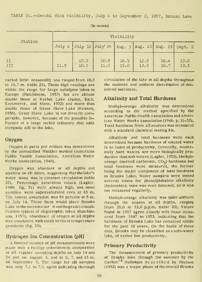
TABLE 21.—Secchi disk visibility, July 4 to September 2, 1957, Brooks Lake

[In meters]

Station

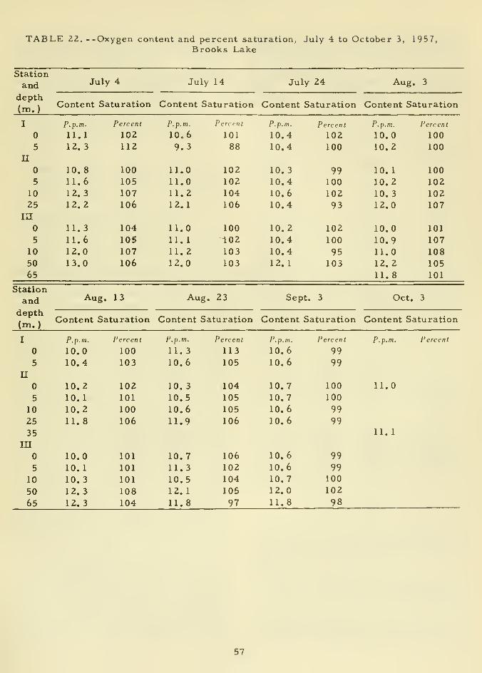
TABLE 22. --

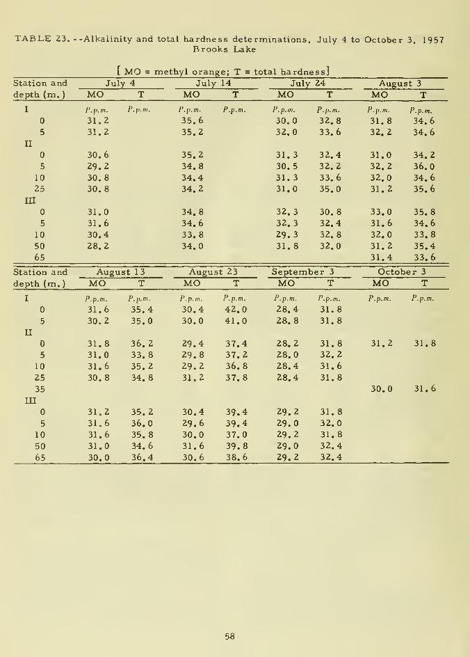
TABLE 23. --Alkalinity and total hardness determinations, July 4 to October 3, 1957Brooks Lake

[ MQ = methyl orange; T = total hardness]Station

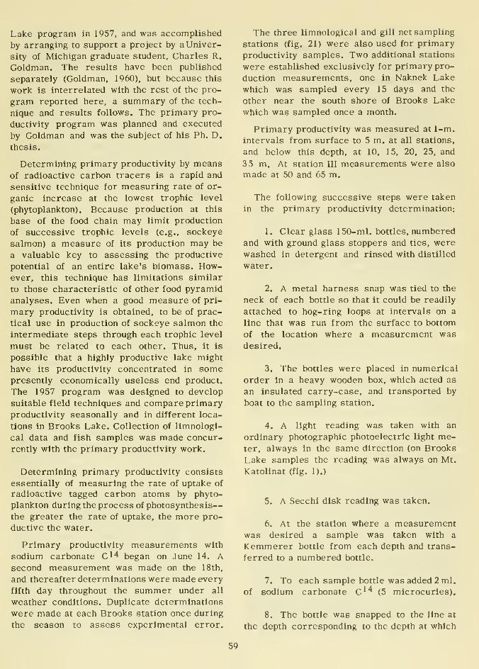
Lake program in 1957, and was accomplished

by arranging to support a project by a Univer-

sity of Michigan graduate student, Charles R.

Goldman. The results have been published

separately (Goldman, 1960), but because this

work is interrelated with the rest of the pro-

gram reported here, a summary of the tech-

nique and results follows. The primary pro-

ductivity program was planned and executed

by Goldman and was the subject of his Ph. D.

thesis.

Determining primary productivity by meansof radioactive carbon tracers is a rapid and

sensitive technique for measuring rate of or-

ganic increase at the lowest trophic level

(phytoplankton). Because production at this

base of the food chain may limit production

of successive trophic levels (e.g., sockeye

salmon) a measure of its production may be

a valuable key to assessing the productive

potential of an entire lake's biomass. How-ever, this technique has limitations similar

to those characteristic of other food pyramidanalyses. Even when a good measure of pri-

mary productivity is obtained, to be of prac-

tical use in production of sockeye salmon the

intermediate steps through each trophic level

must be related to each other. Thus, it is

possible that a highly productive lake might

have its productivity concentrated in somepresently economically useless end product.

The 1957 program was designed to develop

suitable field techniques and compare primaryproductivity seasonally and in different loca-

tions in Brooks Lake. Collection of limnologi-

cal data and fish samples was made concur-

rently with the primary productivity work.

Determining primary productivity consists

essentially of measuring the rate of uptake of

radioactive tagged carbon atoms by phyto-

plankton during the process of photosynthesis

—

the greater the rate of uptake, the more pro-

ductive the water.

Primary productivity measurements with

sodium carbonate C'^ began on June 14. Asecond measurement was made on the 18th,

and thereafter determinations were made every

fifth day throughout the summer under all

weather conditions. Duplicate determinations

were made at each Brooks station once during

the season to assess experimental error.

The three limnological and gill net sampling

stations (fig, 21) were also used for primary

productivity samples. Two additional stations

were established exclusively for primary pro-

duction measurements, one in Naknek Lake

which was sampled every 15 days and the

other near the south shore of Brooks Lake

which was sampled once a month.

Primary productivity was measured at 1-m,

intervals from surface to 5 m. at all stations,

and below this depth, at 10, 15, 20, 25, and

3 5 m, At station III measurements were also

made at 50 and 65 m.

The following successive steps were taken

in the primary productivity determination;

1. Clear glass 150-ml, bottles, numberedand with ground glass stoppers and ties, were

washed in detergent and rinsed with distilled

water.

2. A metal harness snap was tied to the

neck of each bottle so that it could be readily

attached to hog-ring loops at intervals on a

line that was run from the surface to bottom

of the location where a measurement wasdesired.

3. The bottles were placed in numerical

order in a heavy wooden box, which acted as

an insulated carry-case, and transported by

boat to the sampling station,

4. A light reading was taken with an

ordinary photographic photoelectric light me-ter, always in the same direction (on Brooks

Lake samples the reading was always on Mt.

Katolinat (fig. 1).)

5. A Secchi disk reading was taken.

6. At the station where a measurementwas desired a sample was taken with a

Kemmerer bottle from each depth and trans-

ferred to a numbered bottle.

7. To each sample bottle was added 2 ml,

of sodium carbonate C^"* (5 microcuries).

8. The bottle was snapped to the line at

the depth corresponding to the depth at which

59

the sample was taken, and the series of bottles

was then lowered to incubating depths.

9. Samples were allowed to incubate for

4 hours at the selected depths,

10. In the same sequence as incubation

was started, bottles were picked up at the

end of 4 hours and immediately placed in the

dark sample box.

11. Samples were rushed back to the

laboratory, and 100 ml. of each were vacuum-filtered through millipore filters again in the

same order as originally set out.

12. Very dilute Janus Green B dye (2 ml.)

was added to the sample being filtered to detect

leaks in the vacuum system.

13. Ten ml, 0,003 HCL (normal) werepipetted onto the filter to remove residual

carbonate or organisms adhering to the funnel

surface.

14. Ten ml, 3 percent formalin werepipetted onto the filter to preserve organismsand prevent bacterial activity,

15. The millipore filters were placed in

individual shallow aluminum sample pans to

dry.

16. Millipore filters were glued to shallow

sample pans, on the back of which were in-

scribed the station, date, depth, and ml. of

sample (if different from 100 ml. normal).

17. Sample pans were mailed to the Uni-

versity of Michigan where radiation of each

was later measured.

An example of one series of comparativedata between Naknek and Brooks Lakes demon-strates a typical situation (fig. 36). Produc-tivity is measured in terms of beta radiation

counts per second. Highly turbid Naknek Lakeis much more productive than clear BrooksLake in the upper 10 m., but below that depth,

because of deeper light penetration. BrooksLake is the more productive. The striking

differences shown are all the more significant

when one considers that Brooks Lake tempera-tures were higher (which would increase

production) and that the Brooks experiment wason a bright day, while that for Naknek Lakewas on a cloudy day. This example served to

10

a. 20ua

25

30

35

<>

summer period continues year around, wemust search for causes other than lack of

dissolved nutrients to explain Brooks Lake's

low fish production.

TEMPERATURE OF BROOKS RIVERAND ONE SHOT CREEK

Thermographs were operated continuously

as in previous years on Brooks River and OneShot Creek to record water temperatures.

Solar radiation in terms of incident radia-

tion in gram calories per square centimeter

was recorded continuously during the last part

of the summer with a pyrheliometer. These

data will be extremely useful in the future

when several years of comparative seasonal

totals have been collected. The weather in

1957 was exceptionally clear and sunny at

Brooks Lake, and we might expect that phyto-

plankton production would be greater under

such conditions than it would during a cloudy

summer with less solar radiation reaching the

lake's surface.

CLIMATOLOGICAL DATA

A weather station was operated throughout

the summer, recording daily rainfall, maxi-mum and minimum temperatures, 6 p.m.

temperature, and observations of unusual

weather. Data for all year may be found in

"Climato logical Data, Alaska," the monthly

summary published by the U.S. Weather Bureau.

FLUCTUATIONS IN LAKE LEVELA lake-level recorder and still well was in-

stalled on a rock ledge near Brooks Lake outlet

to record fluctuations in Lake level. Its exact

elevation was surveyed to an improvised per-

manent bench mark embedded in the ledge of

the north end of the weir so that when it is

removed for winter storage it can be re-

established each spring at the identical level.

SUMMARY AND CONCLUSIONS

1

.

The adult sockeye salmon run into Brooks

Lake extended from June 25 to October 4 with

a peak migration in early July.

2. The 1957 run of 31,597 sockeye salmon

was one of the smallest spawning escapements

since 1940 when counting began. After recount-

ing 27,183 downstream, a nettotalof only 4,414

remained in the lake. This total proved to be

incorrect.

6. A sample of 704 adult sockeye salmon

was taken at the weir to determine the age and

length composition, sex ratio, and potential egg

deposition of the run.

7. Age composition of the run was: 27 per-

cent 59. 8.1 percent 5o, and 62.1 percent 6„.

8. The sex ratio of the 1957 adult run was1:1.

3. Many sockeye salmon escaped upstreamunobserved; the true escapement was esti-

mated to be 29,000 sockeye salmon, based on

tagging at the weir and recovery on the spawn-

ing grounds.

4. About half of the sockeye salmon that

entered the lake later returned to spawn in

Brooks River.

5. Other salmon species counted through

the weir were: 7 chum, 18 king, 461 coho,

and 1 pink.

9. Mean mideye-fork length of males sam-pled at the weir was 55.9 cm. and of females,

55.4 cm.

10. Calculated numbers of eggs In female

sockeye salmon in the run ranged from 3,044

to 5,060 per female with a mean of 4,115.

11. Potential egg deposition in the Brooks

Lake system (not Including Brooks River) wasestimated to be 57 million.

61

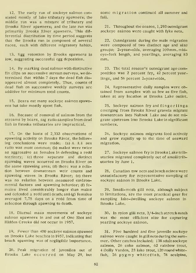
12. The early run of sockeye salmon con-

sisted mostly of lake tributary spawners; the

middle run was a mixture of tributary and

Brooks River spawners; and the late run wasprimarily Brooks River spawners. This dif-

ferential distribution by time period suggests

that the Brooks run is composed of several

races, each with different migratory habits.

13. Egg retention by Brooks spawners is

low, suggesting successful egg deposition.

some migration continued all summer and

fall.

21. Throughout the season, 1,293 outmigrant

sockeye salmon were caught with fyke nets.

22. Outmigrants during the main migration

were composed of two distinct age and size

groups: 2-year-olds, averaging 109 mm. mid-

eye-fork length, and yearlings, averaging 83

mm.

14. By marking dead salmon with distinctive

fin clips on successive stream surveys, we de-

termined that within 7 days the dead fish dis-

appeared almost completely. Thus, counts of

dead fish on successive weekly surveys are

additive for minimum total counts.

15. Bears eat many sockeye salmon spawn-ers but take mostly spent fish.

16. Because of removal of salmon from the

streams by bears, tag ratio samples from dead

fish in Brooks tributaries are impractical.

17. On the basis of 2,333 observations of

spawning activity on Brooks River, the follow-

ing conclusions were made: (a) A 1:1 sex

ratio was most common; (b) males were twice

as aggressive as females in defending a redd

territory; (c) three separate and distinct

spawning waves occurred on Brooks River on

the same spawning area; (d) there was a rela-

tion between downstream weir counts and

spawning waves in Brooks River; (e) there

was no relation between measured environ-

mental factors and spawning behavior; (f) fe-

males lived considerably longer than malesand defended a redd until death; and (g) females

averaged 7.75 days on a redd from time of

selection through spawning to death.

23. The total season's outmigrant age com-position was 2 percent fry, 42 percent year-

lings, and 56 percent 2-year-olds.

24. Representative daily samples were ob-

tained from samples with as few as five fish,

taken at any location at Brooks Lake outlet.

25. Sockeye salmon fry and finge r lingsemerging from Brooks River gravels migrate

downstream into Naknek Lake and do not mi-grate upstream into Brooks Lake in significant

numbers.

26. Sockeye salmon migrants feed actively

and grow rapidly up to the time of seawardmigration.

27. Sockeye salmon fry in Brooks Lake trib-

utaries migrated completely out of small trib-

utaries by June 1,

28. Canadian tow nets and beach seines wereunsatisfactory for representative sampling of

sockeye salmon in Brooks Lake.

29. Small-mesh gill nets, although subject

to limitations, are the most practical gear for

sampling lake-dwelling sockeye salmon in

Brooks Lake.

18. Diurnal mass movements of sockeye

salmon spawners in and out of One Shot and

Hidden Creeks did not occur in 1957.

19. Fewer than 400 sockeye salmon spawnedon Brooks Lake beaches in 1957, indicating that

beach spawning was of negligible importance.

20. Peak migration of juveniles out of

Brooks Lake occurred on May 29, but

30. In nylon gill nets, 3/4-inch stretch meshwas the most efficient size for capturing

yearling sockeye salmon.

31. Five hundred and five juvenile sockeye

salmon were caught in gill nets during the sum-mer. Other catches included: 138 adult sockeye

salmon, 26 coho salmon, 62 rainbow trout,

4 Dolly Varden, 23 lake trout, 120 round white-

fish, 26 pygmy whitefish, 78 sculplns.

62

1 blackfish, 5 ninespine stickleback, and 9

threespine stickleback,

32. Sockeye salmon fry were not success-

fully caught in gill nets because the smallest

mesh size was too large to hold them.

33. Juvenile sockeye salmon were nearly

absent from midlake areas in early summerbut gradually adopted a pelagic life as the

season progressed,

34. In midlake 79 percent of the sockeye

salmon were captured between the surface

and 15 feet, and only 21 percent from 15 to

45 feet,

35. Increases in weight of lake-dwelling

juvenile sockeye salmonleveloff during August

and September when initial formation of an

annulus occurs.

36. Of sockeye salmon caught in the lake

more were feeding on insects than on plankton.

37. Incidence of empty stomachs increased

through the season.

38. Four varieties of zooplankton and one of

insects made up the bulk of sockeye salmonfood in the lake.

39. Sockeye salmon in the lake had no

serious parasite infestations.

40. SCUBA is a practical method of observ-

ing fish in the natural aquatic environment

in Brooks Lake.

41. Brooks Lake zooplankton and phyto-

plankton were well distributed at all depths

and stations through the season and, com-pared with other North American lakes, wererelatively abundant.

42. A large-scale contour map of BrooksLake was completed based on 57 transects

made with an echo sounder.

43. Periodic chemical and physical meas-urements were made of the following water

qualities from surface to bottom at three

stations: temperature, transparency, phos-phorus, nitrogen, silica, turbidity, oxygen, pH,

and total hardness. Each of these was adequate

to support fish and was well distributed at all

depths through the summer.

44. Primary productivity of Brooks Lakewas measured throughout the summer by the

Carbon^^ technique of Nielsen (1952) at 5-day

intervals at three stations from surface to bot-

tom; measurements in Naknek Lake were madeevery 15 days for comparison. Primary pro-

ductivity was moderately low but extended to

a much greater depth in Brooks Lake than in

Naknek. Rate of production in Naknek Lake in

the surface region was greater than in Brooks,

but production in Brooks extended to a greater

depth.

ACKNOWLEDGMENTSThe enthusiasm and technical competence

of the six college students who assisted me at

Brooks Lake made possible the successful

accomplishment of program objectives. Eachassistant was responsible for one phase or

more of the program, and under my direction

each prepared an analysis and report whenthe project was completed. Their reports are

the basis for this paper. Their individual

principal contributions and college or univer-

sity origins are as follows: W. L. Hartman,

Cornell University, contour map and spawning

behavior observations; C. R. Goldman, Uni-

versity of Michigan, primary productivity;

W. H. Pogue, Humboldt State College, counts,

tagging, stream surveys, adult samples, and

climatological instruments; R. E. Painter,

University of Michigan, primary productivity,

spawning observations, and chemical water

analyses; J. A. Harbour, Eastern Washington

College, fingerling outmigration; F. P.Meyer,Iowa State College, gill net sampling, food

studies, upstream migration of juveniles in

Brooks River, plankton, and fish parasites;

G. Y. Wong, University of Washington, chemi-cal water analyses.

63

F. F. Hooper recommended instruments

and procedures for some of the chemical

analyses. Warren Steenberg, Katmai National

Monument Ranger, piloted his personal plane

for aerial surveys of beach spawning on Sep-

tember 14. W. E. Johnson of the Fisheries

Research Board of Canada supplied the Cana-dian tow net.

LITERATURE CITED

AMERICAN PUBLIC HEALTH ASSOCIATION.AMERICAN WATER WORKS ASSOCIA-TION.

1946. Standard methods for the examination

of water and sewage. 9th ed. Lancaster

Press, Inc., Lancaster, Pa., 286 p.

BARNABY, JOSEPH T.

1944. Fluctuations in abundance of red

salmon, Oncorhynchus nerka (Walbaum),

of the Karluk River, Alaska. U.S. Fish

and Wildlife Service, Fishery Bulletin

39, vol. 50, p. 237-295.

BIRGE, E. A., and C. JUDAY.1922. The inland lakes of Wisconsin. The

plankton. I. Its quantity and chemical

composition. Wisconsin Geological and

Natural History Surveys, Bulletin 64,

Science Series No. 13, 222 p.

BRETT, J. R.

1952. Skeena River sockeye escapement and

distribution. Journal of the Fisheries

Research Board of Canada, vol.8, no. 7,

p. 453-468.

CLARK, WEBSTER K.

1957. Seasonal food habits of the Kodiak

bear. Transactions of the Twenty-Sec-

ond North American Wildlife Conference,

p. 145-151

CLARKE, G. L., and D. F. BUMPUS.1950. The plankton sampler—an instrument

for quantitative planktori investigations.

American Society of Limnology and

Oceanography, Special Publication No. 5,

8 p.

EICHER, G. J., Jr.

1951. Effects of tagging on red salmon.

U.S. Fish and Wildlife Service, Special

Scientific Report— Fisheries No. 64, 4 p.

ESCHMEYER, P. H., and R. M.BAILEY.1954. The pygmy whitefish. Core gonus

coulteri, in Lake Superior. Transactions

of the American Fisheries Society, vol.

84, p. 161-199.

FOERSTER, R. E.

1936. An investigation of the life history

and propagation of the sockeye salmon

(Oncorhynchus nerka) at CultUS Lake,

British Columbia. Journal of the Bio-

logical Board of Canada, vol. 2, no. 3,

p. 311-333.

GILBERT, CHARLES H., and WILLIS H.RICH.1927. Investigations concerning the red

salmon runs to the Karluk River, Alaska.

Bulletin of the U.S. Bureau of Fisheries,

vol. 43, p. 1-69. [ Document No. 1021,

issued July 27, 1927.]

GOLDMAN, CHARLES R.

1960. Primary productivity and limiting

factors in three lakes of the Alaska

Peninsula. Ecological Monographs, vol.

30, no. 2 (April), p. 207-230.

GRIGGS, ROBERT F.

1922. The valley of ten thousand smokes.

The National Geographic Society, Wash-ington, D.C., 341 p.

HUTCHINSON, G. E.

1957. A treatise on limnology. John Wileyand Sons, Inc., New York, 1015 p.

CLUTTER, R. 1., and L. E.WHITESEL.1956. Collection and interpretation of

sockeye salmon scales. International

Pacific Salmon Fisheries Commission,Bulletin 9, 159 p.

IDYLL, C.

1942. Food of rainbow, cutthroat and browntrout in the Cowichan River system, B.C.

Journal of the Fisheries Research Boardof Canada, vol. 5, no. 5, p. 448-458.

64

JOHNSON, W. E.

1956. On the distribution of young sockeye

salmon (Oncorhynchus nerha) in Babine

and Nilkitkwa Lakes, B. C. Journal of

the Fisheries Research Board of Canada,

vol. 13, no. 5, p. 695-708.

JUDAY, C, WILLIS H. RICH, G. I. KEM-MERER, and ALBERT MANN.

1932, Limnological studies of Karluk LakeAlaska, 1926-1930. Bulletin of the U.S.

Bureau of Fisheries, vol. 47, no. 12,

p. 407-436.

KROGIUS, F. V.

1951. O dinamike chislennosti krasnoi(Oncorhynchus nerka (Walbaum)). [On the

dynamics of abundance of the sockeye

salmon (Oncorhynchus nerka Walb.).]

Izvestiia Tikhookeanskovo Nauchno-is-

sledovatel'skovo Instituta RybnovoKho-ziaistva i Okeanografii, vol. 35, p. 1-16.

[Fisheries Research Board of Canada,

Translation Series No. 101.] (Transla-

tion examined only.)

KROGIUS, F. v., and E. M. KROKHIN.1948. Ob urozhainosti molodi krasnoi

(Oncorhynchus nerka Walb.) [On the pro-

duction of young sockeye salmon(Oncorhynchus nerka Walb.).] Izvestiia

Tikhookeanskovo Nauchno-is-sledovatel'skovo Instituta RybnovoKhoziaistva \ Okeanografii, vol, 28

p. 3-27. [Fisheries Research Board of

Canada, Translation Series No. 109.]

(Translation examined only.)

1956a. Rezultaty issledovanii biologii nerki-

krasnoi sostoainiia ee zaposov i kole-

banii chislennosti v vodakh Kamchatki.

[Results of a study of the biology of

sockeye salmon, the condition of the

stocks, and the fluctuation in numbersin Kamchatka waters.] Voprosy Ikhtlo-

logii, no. 7, p. 3-20. [Fisheries Re-search Board of Canada, Translation

Series No. 176.] (Translation examined

only.)

1956b. Prichiny kolebanii chislennosti

krasnoi na Kamchatki. [Causes of the

fluctuations in abundance of sockeye

salmon in Kamchatka.] Trudy Problem-nikh i Tematicheskikh Soveshchanii ZIN,

No. 6, p. 144-149. [ Fisheries ResearchBoard of Canada, Translation Series

No. 92.] (Translation examined only.)

LAGLER, KARL F.

1949. Studies in freshwater fishery biology,

3d ed. J. W. Edwards, Ann Arbor, Mich.,

231 p.

1952. Freshwater fishery biology. William

C. Brown Co., Dubuque, Iowa, 360 p.

MATHISEN, OLE A.

1955. Studies on the spawning biology of the

red salmon, Oncorhynchus nerka (Wal-

baum), in Bristol Bay, Alaska, with

special reference to the effect of al-

tered sex ratios. Ph. D. Thesis, Univer-

sity of Washington, Seattle, 285 p.

MILLER, R. B., and W. A. KENNEDY.1946. Observations on the lake trout of

Great Bear Lake. Journal of the Fish-

eries Research Board of Canada, vol.

7, no. 4, p. 176-189.

NIELSEN, E. STEEMANN.1952. The use of radio-active carbon (Cl4)

for measuring organic production in the

sea. Journal du Conseil, Conseil Per-

manent International pour I'Exploration

de la Mer, vol. 18, p. 117-140.

PENNAK, ROBERT W.1953. Freshwater invertebrates of the

United States. The Ronald Press Co.,

New York, 769 p.

RAWSON, D. S.

1951. Studies of the fish of Great Slave

Lake. Journal of the Fisheries Research

Board of Canada, vol. 8, no. 4, p. 207-

240.

1956. The net plankton of Great Slave Lake.

Journal of the Fisheries Research Boardof Canada, vol. 13, no. 1, p. 53-127.

65

REES. W. H.

1957. The vertical and horizontal distribu-

tion of seaward migrant salmon in the

forebay of Baker Dam. Washington De-

partment of Fisheries, Fishery Re-

search Paper, vol. 2, no. 1, p. 5-17.

RICKER, W. E.

1937. Physical and chemical characteris-

tics of Cultus Lake, B. C. Journal of

the Biological Board of Canada, vol. 3,

no. 4, p. 363-402.

1952. The benthos of Cultus Lake. Journal

of the Fisheries Research Board of

Canada, vol. 9, no. 4, p. 204-212.

ROUNSEFELL, GEORGE A,

1957. Fecundity of North American sal-

monidae. U.S. Fish and Wildlife Service,

Fishery Bulletin 122, vol. 57, p. 451-468.

RUTTNER, FRANZ.1953. Fundamentals of limnology. University

of Toronto Press.Toronto, Canada, 242 p.

SCHAEFER, MILNER B.

1951. A study of the spawning populations

of sockeye salmon in the Harrison

River system, with special reference

to the problem of enumeration by means

of marked members. International Pa-

cific Salmon Fisheries Commission,

Bulletin 4, 207 p.

WARNER, KENDALL.1953. The use of a graphic-recording echo

sounder on Maine lakes. Progressive

Fish-Culturist, vol. 15, no. 4, p. 170-

174.

WELCH, PAUL S.

1935. Limnology. McGraw-Hill Book Co.,

New York, 471 p.

1948, Limnological methods. TheBlakiston

Company. Philadelphia, 381 p.

MS #1002

66

MBL WHOI Library - Serials

5 WHSE 01583

Created in 1849 the Department of the Interior—o depart-

ment of conservation— is concerned with the management,

conservation, and development of the Nation's water, fish,

wildlife, mineral, forest, and park and recreational resources.

It also has major responsibilities for Indian and Territorial

affairs.

As the Nation's principal conservation agency, the De-partment works to assure that nonrenewable resources are

developed and used wisely, that park and recreational re-

sources are conserved for the future, and that renewable

resources make their full contribution to the progress, pros-

perity, and security of the United States—now and in the future.

UNITED STATESDEPARTMENT OF THE INTERIOR

FISH AND WILDLIFE SF,RVICE

BUREAU OF COMMERCIAL FISUERIES

WASHINGTON, D.C. 20240

U.S.

POSTAGE AND FEES PAIDDEPARTMENT OF THE INTERIOR

marine Biolosical Lab.,

123 T Woods Hole, Mass.