Ecological Economics: An Analytical Thermodynamic Theory

Jing Chen

School of Business University of Northern British Columbia Prince George, BC Canada V2N 4Z9 Phone: 1-250-960-6480 Fax: 1-250-960-5544 Email: chenj@unbc.ca Web: http://web.unbc.ca/~chenj/

August, 2007 We thank Rongshu Chen, Yaoqi Zhang and participants of 2007 USSEE meeting for helpful comments. Detailed comments from Charles Hall greatly improved the quality of this paper.

1

Abstract

More and more researchers in ecological economics have recognized that the biophysical

approach provides a better foundation to understand human society and its long term evolution

than mainstream economic theory. However, ecological economics textbooks are still written

from the mainstream economics perspective. This is largely due to a lack of analytical theory in

ecological economics. One would expect that an analytical theory based on sound physical

foundation would provide a clearer understanding of our daily activities than mainstream

economics, whose foundation has been challenged by more and more researchers. This is indeed

the case. In this paper, we present a newly developed analytical thermodynamic theory of

ecological economics and show how it provides much more realistic and intuitive understanding

of economic, social and biological phenomena than mainstream economic theory. This theory

turns the insights from ecological economics into an analytical model that can be applied to day

to day business activities. It will help transform ecological economics from a niche subject into

the theoretical foundation of social sciences.

Keywords: ecological economics, analytical thermodynamic theory, cost structure, return

2

1. Introduction

More and more researchers in ecological economics have recognized that the biophysical

approach provides better foundation to understand human society and its long term evolution than

mainstream economic theory. However, ecological economics textbooks are still written from the

perspective of mainstream economics (Stern, 2007). This is largely due to a lack of analytical

theory in ecological economics. One would expect that an analytical theory based on a sound

physical foundation would provide a clearer understanding of our daily activities than mainstream

economics, whose foundation has been challenged by more and more researchers. This is indeed

the case. A newly developed analytical thermodynamic theory of ecological economics provides

much more realistic and intuitive understanding of economic, social and biological phenomena

than mainstream economic theory (Chen, 2005). In this paper, we will present a more detailed

discussion of the production theory, which forms one part of the analytical theory, and show how

the new production theory provides a simple and systematic understanding business investment

problems we encounter frequently.

Because of the fundamental link between thermodynamics and life, many attempts have been

made to develop analytical theories based on the principle of thermodynamics and apply them to

living systems and human society. These include Lorenz’ chaos theory and Prigorgine’s far from

equilibrium thermodynamic theory. Lorenz, a meteorologist, simplified weather equations, which

are thermodynamic equations, into ordinary differential equations. He found chaos properties

from these equations. Prigorgine developed the theory from some chemical reactions. The

theories of Lorenz and Prigorgine greatly influenced the thinking in biology and social sciences.

However, they do not model life process or social activities directly. Chaos theory and

Prigorgine’s theory, while providing good insights to the research in biological and social

sciences, are mostly analogies. Many of the recent works on the application of physics to

3

economics are summarized in Farmer et al. (2005). These works apply the techniques from

research in physics to economics and do not directly model economic activities as physical

processes.

Since uncertainty is an integral part of life processes, the advancement of stochastic calculus is

essential for the development of an analytical thermodynamic theory of life and human society. In

the past several decades, some fundamental works in the area of stochastic calculus were

undertaken by people with very diverse backgrounds. Three works are particularly relevant to the

development of our theory. The first is Ito’s Lemma, which provides a rule to find the differential

of a function of stochastic variable. Ito’s Lemma was obtained in 1940s. But its importance was

not recognized until its wide spread application in financial economics several decades later. Ito

was awarded Gauss Prize in 2006, sixty years after his theory was initially developed.

The second tool is Feynman-Kac formula, which maps a stochastic process into a deterministic

thermodynamic equation. Richard Feynman (1948) attempted to simplify calculation in quantum

mechanics by transforming problems in stochastic processes into problems in deterministic

processes. The new mathematical technique enabled him to perform many computations in

quantum mechanics which were very difficult in the past. With this he established the theory of

quantum electrodynamics. The breakthrough in physics is often generated by the breakthrough in

new mathematical methods, which enables us to describe the subtler parts of the nature. An

important motivation in Feynman’s research was his seek for universality. “The question that then

arose was what Dirac had meant by the phrase ‘analogous to,’ and Feynman determined to find

out whether or not it would be possible to substitute the phrase ‘equal to.’” (Feynman and Hibbs,

1965, p. viii) Feynman, together with Tomonaga and Schwinger, was awarded Nobel Prize in

physics for this work in 1965. Despite its highly technical nature, Feynman-Kac formula is a very

general result and has proved to be extremely useful in many different fields. In particular,

4

Feynman-Kac formula has been widely used in the research in finance recently. It was even

suggested that “Feynman could be claimed as the father of financial economics” (Dixit and

Pindyck, 1994, p. 123).

The third is Black-Scholes (1973) option pricing theory, which provides an analytical formula of

observable variables to price a financial instrument whose payoff depends on a stochastic process.

This is a landmark contribution in social sciences. It shows that a complex economic problem can

be effectively modeled by a stochastic process, a simple and deterministic analytical theory about

it can be developed and much information about it can be obtained through such an analytical

theory. Fischer Black, one of the co-developers of the Black-Scholes theory, was a legendary

figure in finance.

Fischer never took a course in either economics or finance, so he never learned the way you

were supposed to do things. But that lack of training proved to be an advantage, … since the

traditional methods in those fields were better at producing academic careers than new

knowledge. Fischer’s intellectual formation was instead in physics and mathematics, and his

success in finance came from applying the methods of astrophysics. Lacking the ability to run

controlled experiments on the stars, the astrophysist relies on careful observation and then

imagination to find the simplicity underlying apparent complexity. In Fischer’s hands, the

same habits of research turned out to be effective for producing new knowledge in finance.

(Mehrling, 2005, p. 6)

Black-Scholes option theory provides the earliest inspiration in developing an analytical

thermodynamic theory of life and human society. More detailed discussion about its history can

be found in Chen (2005). In the following, we will briefly discuss the basic ideas of this theory.

5

There are two fundamental properties about life. First, living organisms need to extract resources

from the environment to compensate for the continuous loss of resources required to maintain

various functions of life. Second, for an organism to be viable, the total cost of extracting

resources has to be less than the amount of resources extracted (Odum, 1971 and Hall et al,

1986). The second property could be understood as natural selection rephrased from the resource

perspective. The purpose of our work is to derive a self-contained mathematical theory of

production from these two fundamental properties about life.

From the physics perspective, resources can be regarded as low entropy sources (Georgescu-

Roegen, 1971). The entropy law states that systems tend toward higher entropy states

spontaneously. Living systems, as non-equilibrium systems, need to extract low entropy from the

environment to compensate for their continuous dissipation. It can be represented mathematically

by lognormal processes, which contain a growth term and a dissipation term. From the entropy

law, the thermodynamic dissipation of an organic or economic system is spontaneous. The

extraction of low entropy from the environment, however, depends on specific biological or

institutional structures that incur fixed or maintenance costs. Additional variable cost is required

for resource extraction. Higher fixed cost systems generally have lower variable costs. Fixed cost

is largely determined by genetic structure of an organism or design of a project. Variable cost is a

function of environment. From the Feynman-Kac formula, a result widely used in science

literature and increasingly used in finance literature, we derive the thermodynamic equation that

variable cost of a production system should satisfy. An organism survives if the amount of

resources it extracts is higher than the total cost. Similarly, a business survives if its revenue is

higher than the total cost of production. We set the initial condition of the equation so that total

cost is equal to the amount of resource extracted or revenue generated. Then we solve the

thermodynamic equation to derive an analytic formula that explicitly represents the relation

6

among fixed costs, variable costs, uncertainty of the environment, discount rate and the duration

of a production system, which is the core concern in most economic decisions.

It is often suggested that economic theories, for analytical ease and tractability, sacrifice their

relevance to reality (Hall, et al, 2001). This new theory shows that an economic theory based on

the firm foundation of reality is actually analytically easier and more tractable. In this paper, we

show that the analytical representation of various factors in production processes enables us to

directly compute and analyze the returns of different production systems under various kinds of

environment in a simple and systematic way. The results are highly consistent with the empirical

evidences obtained from the vast amount of literature in economics and ecology. Furthermore, the

theory, by putting major factors of production into a single mathematical model, provides precise

insights about the tradeoffs and constraints of various business or evolutionary strategies that are

often lost in intuitive thinking. For example, in the business literature, some emphasize training of

employee, others emphasize cost cutting. But employee training is costly. The tradeoff between

better training and lower cost is often not explicitly discussed in the same literature. Our theory

provides specific suggestion whether more training or cost cutting is more profitable under

different kinds of circumstances.

Mainstream economists pay little attention to the biophysical foundation of human society

because they believe special qualities of human beings will make physical constraints less

relevant. A biophysical approach puts the physical constraint of human society at the center of its

analysis. The validity of a physical theory is best manifested by the existence of a corresponding

mathematical theory that is derived from the most fundamental properties of life and is consistent

with a wide range of patterns observed in both economics and ecology. After all, all physical laws

are represented by mathematical formulas. The computability of the mathematical theory will

7

transform biological science, which include social science as a special case, into an integral part

of physics.

Simplicity and universality are the hallmarks of this theory. All the results in the paper have been

taught at undergraduate classes and the students embrace the ideas enthusiastically. Since all the

results are calculated from simple analytical formulas, they can be reproduced and applied easily

by researchers and students. An Excel file containing all the calculation and graphs in this paper

can be obtained from the author.

This paper is structured as follows. Section 2 presents the derivation of the analytical

thermodynamic theory. Section 3 presents some detailed results from this theory. Section 4

compares the analytical thermodynamic theory with the neoclassical economic theory. Section 5

concludes.

2. An analytical thermodynamic theory of production

The theory described in this section, which is adapted from Chen (2005), can be applied to both

biological and economic systems. For simplicity of exposition, we will use the language of

economics. But the extension to biological system is straight forward and is consistent with the

ideas put forth by Odum, (1971) and Hall et al, (1986).

A basic property in economic activities is uncertainty. While a business may face many different

kinds of uncertainty, most of the uncertainties are reflected in the price uncertainty of the product.

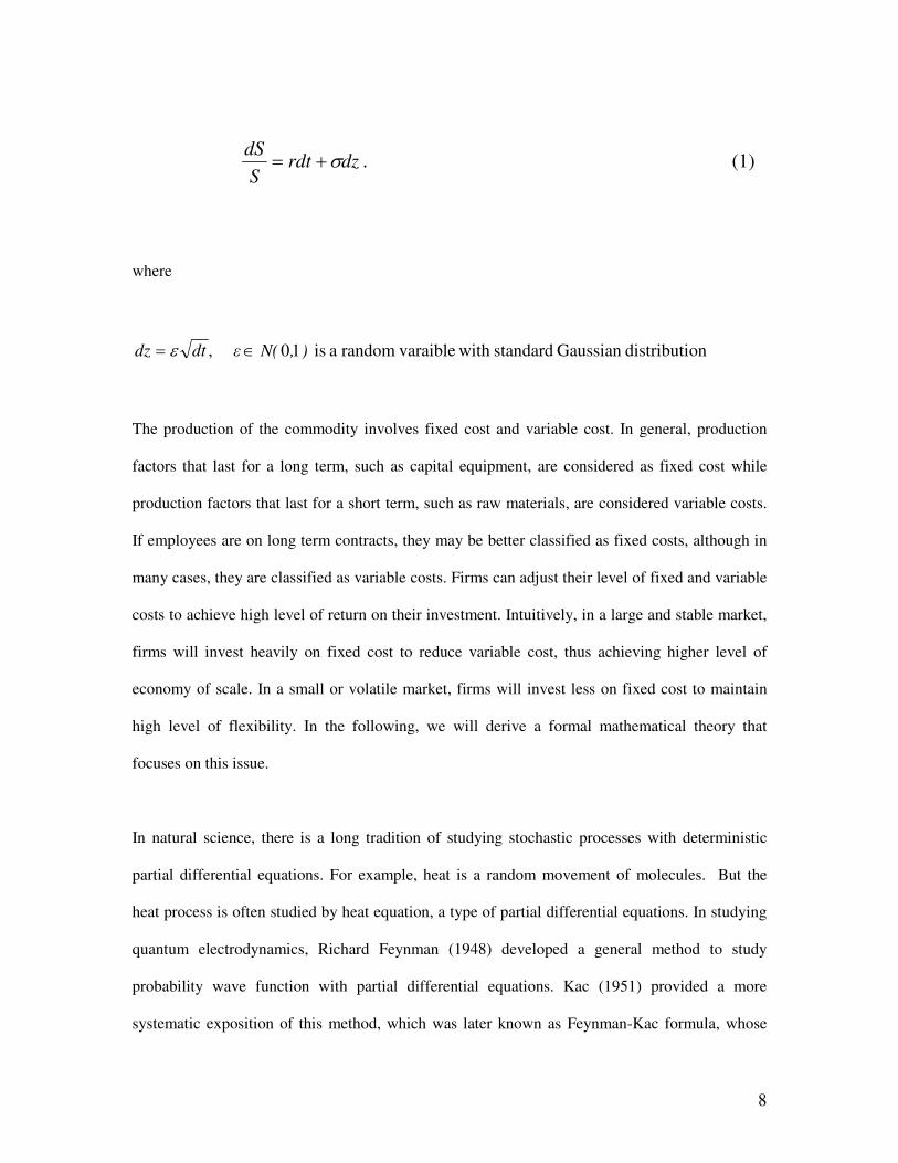
Suppose S represents unit price of a commodity, r, the expected rate of change of price and σ, the

rate of uncertainty. Then the process of S can be represented by the lognormal process

8

where

ondistributiGaussian standard with varaiblerandom a is 10 , ),N(εdtdz ∈= ε

The production of the commodity involves fixed cost and variable cost. In general, production

factors that last for a long term, such as capital equipment, are considered as fixed cost while

production factors that last for a short term, such as raw materials, are considered variable costs.

If employees are on long term contracts, they may be better classified as fixed costs, although in

many cases, they are classified as variable costs. Firms can adjust their level of fixed and variable

costs to achieve high level of return on their investment. Intuitively, in a large and stable market,

firms will invest heavily on fixed cost to reduce variable cost, thus achieving higher level of

economy of scale. In a small or volatile market, firms will invest less on fixed cost to maintain

high level of flexibility. In the following, we will derive a formal mathematical theory that

focuses on this issue.

In natural science, there is a long tradition of studying stochastic processes with deterministic

partial differential equations. For example, heat is a random movement of molecules. But the

heat process is often studied by heat equation, a type of partial differential equations. In studying

quantum electrodynamics, Richard Feynman (1948) developed a general method to study

probability wave function with partial differential equations. Kac (1951) provided a more

systematic exposition of this method, which was later known as Feynman-Kac formula, whose

(1) . dzrdtS

dSσ+=

9

use is very common in natural sciences (Kac, 1985). Recently, Feynman-Kac formula has been

widely used in the research in finance. What I want to do is to apply Feynman-Kac formula to

derive variable cost in production as a function of other parameters.

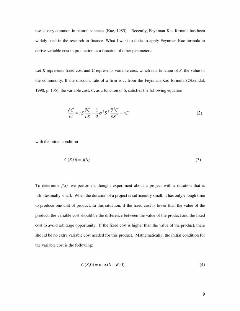
Let K represents fixed cost and C represents variable cost, which is a function of S, the value of

the commodity. If the discount rate of a firm is r, from the Feynman-Kac formula (Øksendal,

1998, p. 135), the variable cost, C, as a function of S, satisfies the following equation

with the initial condition

To determine f(S), we perform a thought experiment about a project with a duration that is

infinitesimally small. When the duration of a project is sufficiently small, it has only enough time

to produce one unit of product. In this situation, if the fixed cost is lower than the value of the

product, the variable cost should be the difference between the value of the product and the fixed

cost to avoid arbitrage opportunity. If the fixed cost is higher than the value of the product, there

should be no extra variable cost needed for this product. Mathematically, the initial condition for

the variable cost is the following:

(2) 2

12

222

rCS

CS

S

CrS

t

C−

∂

∂+

∂

∂=

∂

∂σ

(3) )0,( f(S) SC =

(4) )0,max()0,( KSSC −=

10

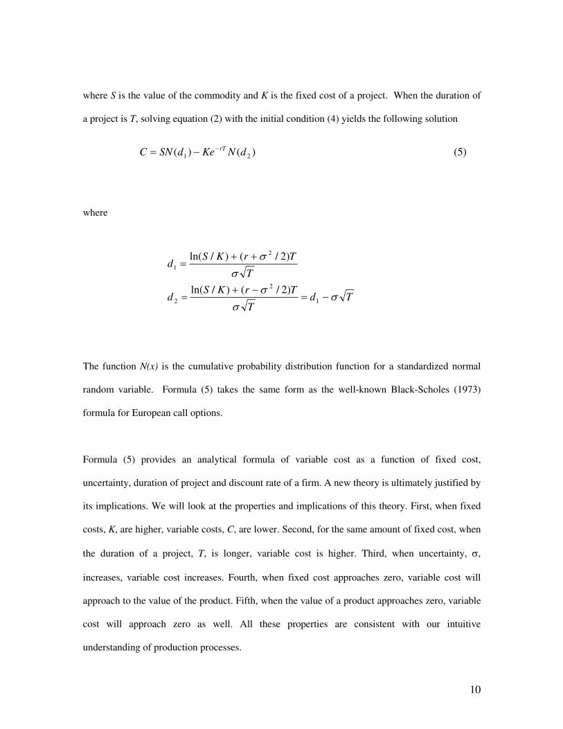
where S is the value of the commodity and K is the fixed cost of a project. When the duration of

a project is T, solving equation (2) with the initial condition (4) yields the following solution

where

The function N(x) is the cumulative probability distribution function for a standardized normal

random variable. Formula (5) takes the same form as the well-known Black-Scholes (1973)

formula for European call options.

Formula (5) provides an analytical formula of variable cost as a function of fixed cost,

uncertainty, duration of project and discount rate of a firm. A new theory is ultimately justified by

its implications. We will look at the properties and implications of this theory. First, when fixed

costs, K, are higher, variable costs, C, are lower. Second, for the same amount of fixed cost, when

the duration of a project, T, is longer, variable cost is higher. Third, when uncertainty, σ,

increases, variable cost increases. Fourth, when fixed cost approaches zero, variable cost will

approach to the value of the product. Fifth, when the value of a product approaches zero, variable

cost will approach zero as well. All these properties are consistent with our intuitive

understanding of production processes.

)2/()/ln(

)2/()/ln(

1

2

2

2

1

TdT

TrKSd

T

TrKSd

σσ

σ

σ

σ

−=−+

=

++=

(5) )()( 21 dNKedSNC rT−−=

11

Suppose the volume of output during the project life is Q, which is bound by production capacity

or market size. We assume the present value of the product to be S and variable cost to be C

during the project life. Then the total present value of the product and the total cost of production

are

respectively. The return of this project can be represented by

and the net present value of the project is

(8) )()( KCSQKQCQS −−=+−

Unlike a conceptual framework, this mathematical theory enables us to make quantitative

calculation of returns of different projects under different kinds of environments. We will provide

a systematic analysis in the next section.

3. Systematic analysis of the performance of a project

The profit or return of a project is determined by fixed cost, variable cost and total output during

the life of the project. Variable cost is a function of fixed cost, uncertainty, duration of the

project, and discount rate. Since how much to invest or commit at the beginning of the project is

the most important decision to make, we will first discuss how fixed cost is related to uncertainty,

(6) and KCQSQ +

(7) ) ln( KCQ

SQ

+

12

duration of the project, discount rate and total output in determining the performance of the

project. Then we will discuss how other factors are related to each other.

Fixed cost and uncertainty:

Calculating variable costs from (5), we find that, as fixed costs are increased, variable costs

decrease rapidly in a low market uncertainty environment and change very little in a high market

uncertainty environment. Put it in another way, high fixed cost systems are very sensitive to the

change of market uncertainty level while low fixed cost systems are not. This is illustrated in

Figure 1.

The above calculation indicates that higher fixed investment is more effective in a low

uncertainty environment and lower fixed cost investment is more flexible in high uncertainty

environment. This explains mature industries, such as household supplies, are dominated by large

companies such as P&G while innovative industries, such as IT, are pioneered by small and new

firms. Microsoft, Apple, CISCO, Yahoo, Google and countless other innovative businesses are

started by one or two individuals and not by established firms. Despite the financial and technical

clout of large firms, small firms account for a disproportionately high share of innovative activity

(Acs and Audretsch, 1990).

Similarly, in scientific research, mature areas are generally dominated by top researchers from

elite schools, while scientific revolutions are often initiated by newcomers or outsiders (Kuhn,

1996).

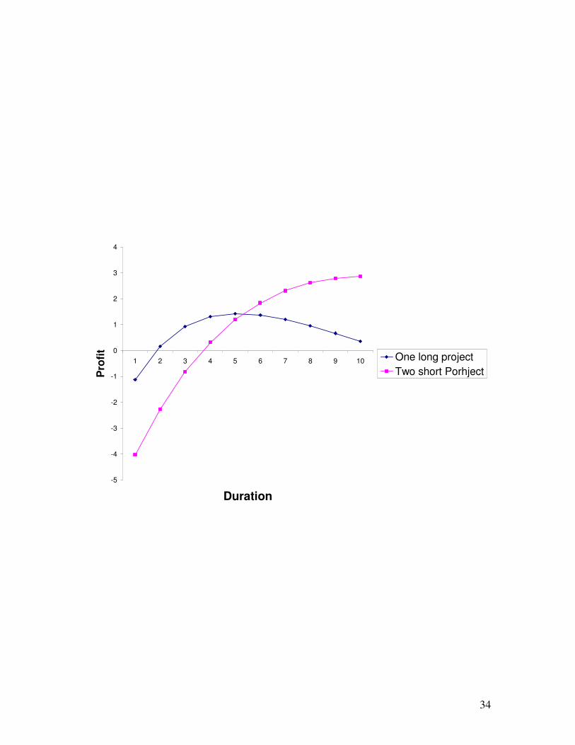
Fixed cost and duration of the project:

13

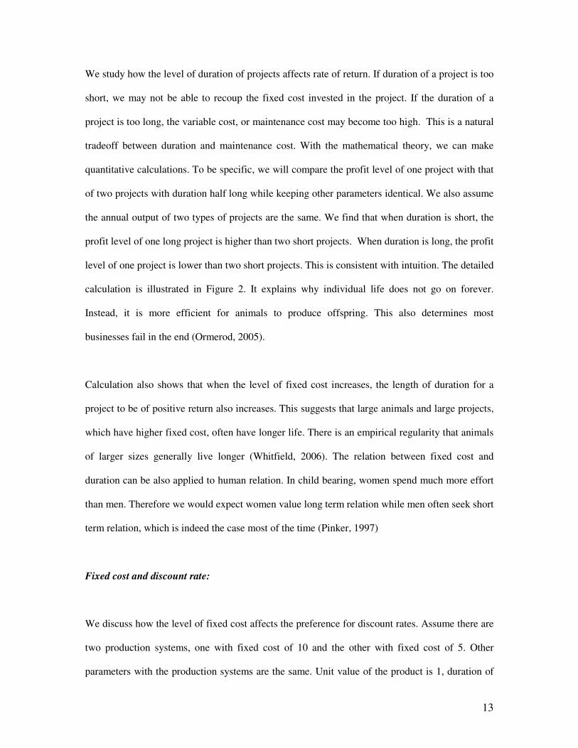
We study how the level of duration of projects affects rate of return. If duration of a project is too

short, we may not be able to recoup the fixed cost invested in the project. If the duration of a

project is too long, the variable cost, or maintenance cost may become too high. This is a natural

tradeoff between duration and maintenance cost. With the mathematical theory, we can make

quantitative calculations. To be specific, we will compare the profit level of one project with that

of two projects with duration half long while keeping other parameters identical. We also assume

the annual output of two types of projects are the same. We find that when duration is short, the

profit level of one long project is higher than two short projects. When duration is long, the profit

level of one project is lower than two short projects. This is consistent with intuition. The detailed

calculation is illustrated in Figure 2. It explains why individual life does not go on forever.

Instead, it is more efficient for animals to produce offspring. This also determines most

businesses fail in the end (Ormerod, 2005).

Calculation also shows that when the level of fixed cost increases, the length of duration for a

project to be of positive return also increases. This suggests that large animals and large projects,

which have higher fixed cost, often have longer life. There is an empirical regularity that animals

of larger sizes generally live longer (Whitfield, 2006). The relation between fixed cost and

duration can be also applied to human relation. In child bearing, women spend much more effort

than men. Therefore we would expect women value long term relation while men often seek short

term relation, which is indeed the case most of the time (Pinker, 1997)

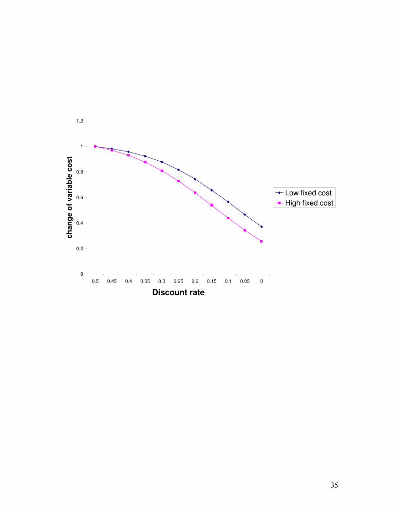
Fixed cost and discount rate:

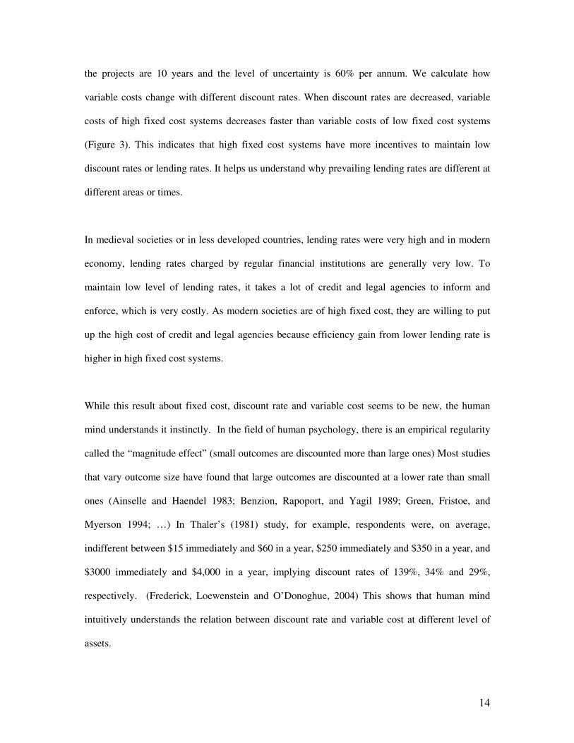
We discuss how the level of fixed cost affects the preference for discount rates. Assume there are

two production systems, one with fixed cost of 10 and the other with fixed cost of 5. Other

parameters with the production systems are the same. Unit value of the product is 1, duration of

14

the projects are 10 years and the level of uncertainty is 60% per annum. We calculate how

variable costs change with different discount rates. When discount rates are decreased, variable

costs of high fixed cost systems decreases faster than variable costs of low fixed cost systems

(Figure 3). This indicates that high fixed cost systems have more incentives to maintain low

discount rates or lending rates. It helps us understand why prevailing lending rates are different at

different areas or times.

In medieval societies or in less developed countries, lending rates were very high and in modern

economy, lending rates charged by regular financial institutions are generally very low. To

maintain low level of lending rates, it takes a lot of credit and legal agencies to inform and

enforce, which is very costly. As modern societies are of high fixed cost, they are willing to put

up the high cost of credit and legal agencies because efficiency gain from lower lending rate is

higher in high fixed cost systems.

While this result about fixed cost, discount rate and variable cost seems to be new, the human

mind understands it instinctly. In the field of human psychology, there is an empirical regularity

called the “magnitude effect” (small outcomes are discounted more than large ones) Most studies

that vary outcome size have found that large outcomes are discounted at a lower rate than small

ones (Ainselle and Haendel 1983; Benzion, Rapoport, and Yagil 1989; Green, Fristoe, and

Myerson 1994; …) In Thaler’s (1981) study, for example, respondents were, on average,

indifferent between $15 immediately and $60 in a year, $250 immediately and $350 in a year, and

$3000 immediately and $4,000 in a year, implying discount rates of 139%, 34% and 29%,

respectively. (Frederick, Loewenstein and O’Donoghue, 2004) This shows that human mind

intuitively understands the relation between discount rate and variable cost at different level of

assets.

15

Differences in fixed costs in child bearing between women and men also affect the differences in

discount rates between them. Women spend much more effort in child bearing. From our theory,

the high fixed investment women put in child bearing would make women’s discount rate lower

than men’s. A classroom survey showed that this is indeed the case.

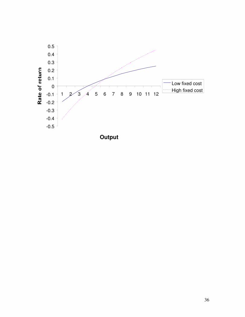
Fixed cost and the volume of output or market size:

We discuss the returns of investment on projects of different fixed costs with respect to the

volume of output or market size. Figure 4 is the graphic representation of (7) for different levels

of fixed costs. In general, higher fixed cost projects need higher output volume to breakeven. At

the same time, higher fixed cost projects, which have lower variable costs in production, earn

higher rates of return in large markets.

From the above discussion the level of fixed investment in a project depends on the expectation

of the level of uncertainty of production technology and the size of the market. When the outlook

is stable and market size is large, projects with high fixed investment earn higher rates of return.

When the outlook is uncertain or market size is small, projects with low fixed cost breakeven

easier.

In ecological system, the market size can be understood as the size of resource base. When

resource is abundant, an ecological system can support large, complex organisms (Colinvaux,

1978). Physicists and biologists are often puzzled by the apparent tendency for biological systems

to form complex structures, which seems to contradict the second law of thermodynamics

(Schneider and Sagan, 2005). However, once we realize that systems of higher fixed cost are

more competitive in the resource rich and stable environments, this evolutionary pattern becomes

easy to understand.

16

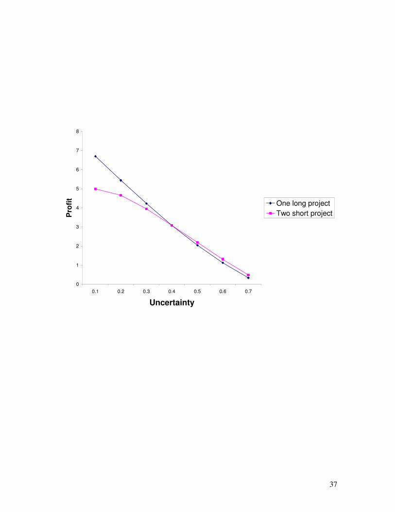
Uncertainty and duration:

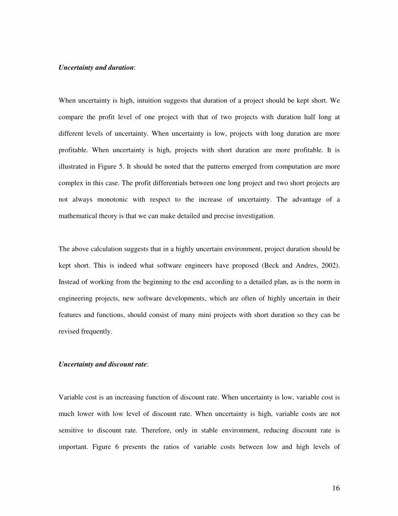
When uncertainty is high, intuition suggests that duration of a project should be kept short. We

compare the profit level of one project with that of two projects with duration half long at

different levels of uncertainty. When uncertainty is low, projects with long duration are more

profitable. When uncertainty is high, projects with short duration are more profitable. It is

illustrated in Figure 5. It should be noted that the patterns emerged from computation are more

complex in this case. The profit differentials between one long project and two short projects are

not always monotonic with respect to the increase of uncertainty. The advantage of a

mathematical theory is that we can make detailed and precise investigation.

The above calculation suggests that in a highly uncertain environment, project duration should be

kept short. This is indeed what software engineers have proposed (Beck and Andres, 2002).

Instead of working from the beginning to the end according to a detailed plan, as is the norm in

engineering projects, new software developments, which are often of highly uncertain in their

features and functions, should consist of many mini projects with short duration so they can be

revised frequently.

Uncertainty and discount rate:

Variable cost is an increasing function of discount rate. When uncertainty is low, variable cost is

much lower with low level of discount rate. When uncertainty is high, variable costs are not

sensitive to discount rate. Therefore, only in stable environment, reducing discount rate is

important. Figure 6 presents the ratios of variable costs between low and high levels of

17

uncertainty at different levels of discount rates. It shows that the reduction of variable cost is

much more significant at low discount rate level.

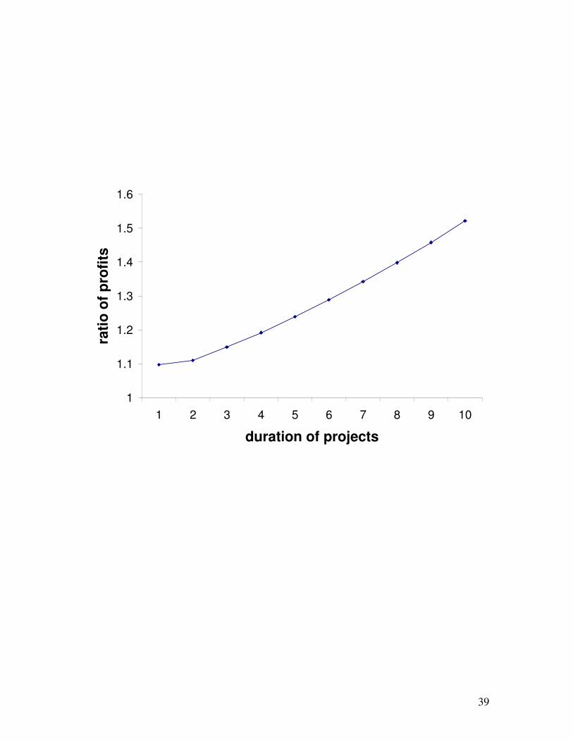
Project duration and discount rate:

When discount rate or interest rate becomes lower, the variable cost of a project will decrease and

profit will increase. Projects with different lengths of duration will be affected differently from

the reduction of discount rates. Figure 7 presents the ratios of profits between projects at low and

high discount rates at different levels of project duration. As project lengths are increases, the

ratios increase as well. This indicates that projects with longer duration benefit more from the

reduction of interest rates.

We next calculate the breakeven point of a project with respect to project duration and discount

rate. Assume that project output per unit time is one. Calculation from formula (7) shows that it

requires lower discount rate to breakeven when project duration is lengthened. When project

duration is sufficient long, the discount rate could become negative at the breakeven point. This is

illustrated in Figure 8. In ecological systems, animals live a long life, such as elephants, generally

have much lower fertility rates than animals live a short life, such as cats. In human society, we

often use longevity, or duration of human life as an indicator of the quality of a social

environment. At the same time, societies enjoy long life span, such as Japan, are often concerned

about below replacement fertility. Our calculation shows that there is negative relation between

duration of life and fertility. Intuitively, aging population needs great amount of resource on

health, which reduces the amount of resources available to support children. Hence, there is a

natural tradeoff between longevity and fertility.

4. A Comparison with Neoclassical Economic Theory

18

Since its birth, the foundation or “assumptions” of neoclassical economic theory has been

criticized for its lack of relevance to reality. To this, Milton Friedman replied:

In so far as a theory can be said to have “assumptions” at all, and in so far as their “realism”

can be judged independently of the validity of predictions, the relation between the

significance of a theory and the “realism” of its “assumptions” is almost the opposite of that

suggested by the view under criticism. Truly important and significant hypotheses will be

found to have “assumptions” that are wildly inaccurate descriptive representations of reality,

and in general, the more significant the theory, the more unrealistic the assumptions (in this

sense). The reason is simple. A hypothesis is important if it “explains” much by little, that is,

if it abstracts the common and crucial elements from the mass of complex and detailed

circumstances surrounding the phenomena to be explained and permits valid predictions on

the basis of them alone. To be important, therefore, a hypothesis must be descriptively false in

its assumptions; it takes account of, and accounts for, none of the many other attendant

circumstances, since its very success shows them to be irrelevant for the phenomena to be

explained. (Friedman, 1953, p. 16)

He further challenged:

As we have seen, criticism of this type is largely beside the point unless supplemented by

evidence that a hypothesis in one or another of these respects from the theory being criticized

yield better predictions for as wide a range of phenomena. (Friedman, 1953, p. 31)

19

Chen (2005) offered very detailed discussion on how the new theory, which is based on more

realistic assumptions, does “yield better predictions for as wide a range of phenomena”. The

following is adapted from Chen (2005), which compares the new production theory briefly with

neoclassical economic theory.

Consistency with physical and biological theories

Neoclassical economics was founded around 1870 by Jevons, Walras and others, who believed

that economics should be built on a sound physical foundation. Since the dominant platform of

physics in Jevons and Walras’ time was Newtonian mechanics, it was natural for them to adopt

this platform. However, theories derived from rational mechanics often do not offer good

explanation to economic behaviors. Gradually, explicit identification with physics disappears

while analogies between physics and economics are frequently mentioned. The following quote

from Samuelson’s Nobel lecture is quite representative:

There is really nothing more pathetic than to have an economist or a retired engineer try to

force analogies between the concepts of economics. How many dreary papers have I had to

referee in which the author is looking for something that corresponds to entropy or to one or

another form of energy.

In the very next paragraph, however, Samuelson found some analogy himself.

However, if you look upon the monopolistic firm hiring ninety-nine inputs as an example of a

maximum system, you can connect up its structural relations with those that prevail for an

20

entropy-maximizing thermodynamic system. Pressure and volume, and for that matter

absolute temperature and entropy, have to each other the same conjugate or dualistic relation

that the wage rate has to labor or the land rent has to acres of land.

Mirowski observed, “The key to the comprehension of Samulson’s meteoric rise in the economics

profession was his knack for evoking all the outward trapping and ornament of science without

ever coming to grips with the actual content or implications of physical theory for his neoclassical

economics” (Mirowski, 1989, p. 383).

Life systems are non-equilibrium thermodynamic systems. The current dominant economic

theory is general equilibrium theorem. Social system is a special case of living systems. When a

theory about a special case is inconsistent with general foundation, either the general foundation

or the special theory is wrong. So far, economists have not challenged the validity of the non-

equilibrium thermodynamic theory of life systems. This theory shows that an analytical theory of

economics can be directly derived from basic physical and biological laws. By this, it establishes

social sciences as an integral part of physical and biological sciences.

A comparison with production functions

Production functions, such as Cobb-Douglas production function, form the fundamental blocks in

general equilibrium production theory. Cobb-Douglas function takes the form

βα KALY =

21

where Y, L and K denote output, labor (variable cost) and capital (fixed cost) respectively. Solow

had made following comment about the production function:

I have never thought of the macroeconomic production function as a rigorously justifiable

concept. In my mind it is either an illuminating parable, or else a mere device for handling

data, to be used so long as it gives good empirical results, and to be discarded as soon as it

doesn’t, or as something better comes along. (Solow, 1966, p. 1259)

By contrast, the analytical production theory developed here is derived rigorously from the

fundamental property of life systems. It gives simple and clear results of returns to investment

under different market conditions. The form and parameters of Cobb-Douglas function are given

without rigorous justification. A, the coefficient in Cobb-Douglas function, “has been called,

among other things, ‘technical change’, ‘total factor productivity’, ‘the residual’ and ‘the measure

of our ignorance’” (Blaug, 1980, p. 465).

From Cobb-Douglas production function, economic output can always be increased by the

increase of capital. This is the basis of continuous economic growth from the neoclassical

economic theory. From the biophysical theory, the return of an economic system can be measured

by formula (7), in which the output of the whole society is considered as a giant project. From

(7), the total output is SQ, which is constrained by the total amount of resources. If K, the total

amount of capital, is too high, the return will become negative and economic activity will shrink

instead of expand over time.

22

Since production functions are widely used in economic literature in constructing economic

models, even a small improvement on this topic should have a big impact in understanding

economics.

Optimality vs. tradeoff

Optimization theory holds the central position in neoclassical economics. Paul Samuelson’s

Nobel Lecture is titled Maximum Principles in Analytical Economics. Alchian (1950) and

Friedman (1953) tried to reconcile the maximization principle with evolutionary theory. Friedman

stated:

Confidence in the maximization-of-return hypothesis is justified by evidence of a very

different character. … unless the behavior of businessmen in some way or other approximated

behavior consistent with the maximization of returns, it seems unlikely that they would remain

in business for long. Let the apparent immediate determinant of business behavior be anything

at all --- habitual reaction, random chance, or whatnot. Whenever this determinant happens to

lead to behavior consistent with rational and maximization of returns, the business will

prosper and acquire resources with which to expand; whenever it does not, the business tend

to lose resources and can be kept in existence only with addition of resources from outside.

The process of “natural selection” thus helps to validate the hypothesis --- or rather, given

natural selection, acceptance of the hypothesis can be based largely on the judgment that it

summarized appropriately the conditions for survival. (Friedman, 1953, p. 22)

23

We will use an example of project investment to illustrate the problem of Friedman’s argument.

Assume the relevant parameters are unit value of the product to be one million, discount rate to be

4%, diffusion to be 40%, duration of the project, to be thirty years and market size to be 150 over

the project life. It can be calculated from Formula (7) that a project with a fixed cost of 25 million

dollar will have the highest rate of return. However, if any parameter changes, the optimal value

of fixed cost investment will change as well. For example, if diffusion increases to 60%, the

optimal value of fixed investment will become 11 million. Since fixed cost is spent or committed

at the beginning of the project while other parameters may change over the course of project life,

it is impossible to determine optimality in advance. Furthermore, higher fixed cost systems,

which are often the winners of earlier market competition, suffer more from the increase of

uncertainty. This means that long term survival is not necessarily consistent with short term

optimization.

Earlier, we have shown that systems with higher fixed costs earn higher rates of return in large

markets and stable environments than those with lower fixed costs. These systems may appear

superior. However, the performance of high fixed cost systems deteriorates in high volatile

environments. From this production theory, the main theme of economic and biological evolution

is the tradeoff between competitiveness of high fixed cost systems in a stable environment and

flexibility of low fixed cost systems in a volatile environment. Biologists haven’t found a

universally applicable measure of fitness (Stearns, 1992, p. 33). Our theory shows that there does

not exist such a measure. For the same reason, there will not exist a universally applicable

measure of optimality.

Is marginal cost equal to marginal revenue?

24

Traditional economic theory suggests that companies will keep increasing the output until the

marginal cost of the product is equal to its marginal revenue (Friedman, 1953, p. 16). Empirical

evidences show that companies generally charge a substantial price mark up on their products.

This analytical theory offers a simple and clear understanding about price markup. For example,

if a software is targeted to sophisticated users, its interface can be simple, which reduce

development cost and its sales effort can be small, which reduce variable cost. If the software

developer considers increasing the market size by targeting general users, the interface of the

software needs to be very intuitive with many help facilities, which increase development cost

and its sales effort and after sales service can be substantial for less sophisticated users, which

increase variable cost. Since the increase of market size often involve both the increase of

variable cost and fixed cost, most projects are designed that the marginal cost to be much lower

than the product value to maximize potential profit.

To keep increasing the output until its marginal cost equal to marginal revenue often means that

the company may have to enter difficult areas, which will have repercussion on its earlier units.

For example, when employees in a WalMart store in Quebec voted to unionize, WalMart closed

down that store although that store would remain profitable under unionized workforce. To keep

a unionized store open will affect the margin of other stores, whose staff will attempt to unionize

as well. From Formula (7), the rate of return not only depends on the market size, but also

depends on other factors. If the increase of market size will increase the diffusion rate as well,

companies have to consider the total effect on long term profitability. To make it more concrete,

we will provide an example.

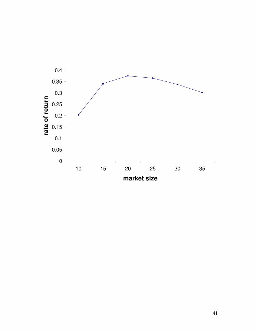
25

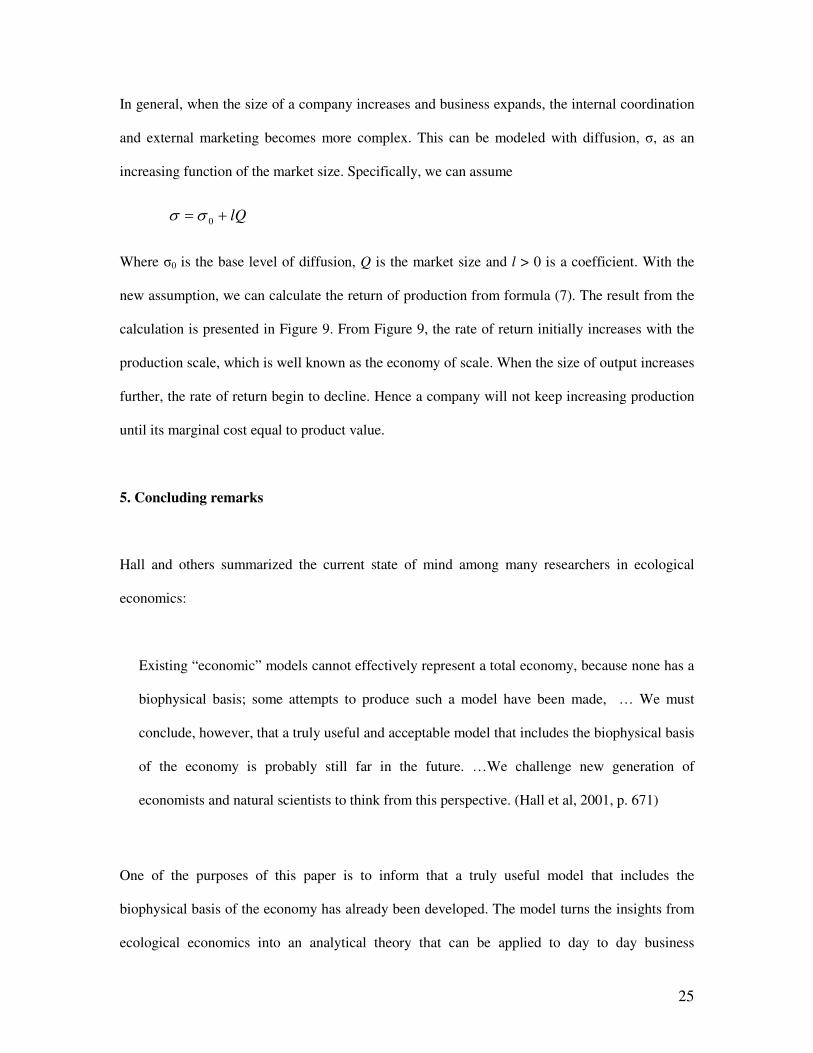
In general, when the size of a company increases and business expands, the internal coordination

and external marketing becomes more complex. This can be modeled with diffusion, σ, as an

increasing function of the market size. Specifically, we can assume

lQ+= 0σσ

Where σ0 is the base level of diffusion, Q is the market size and l > 0 is a coefficient. With the

new assumption, we can calculate the return of production from formula (7). The result from the

calculation is presented in Figure 9. From Figure 9, the rate of return initially increases with the

production scale, which is well known as the economy of scale. When the size of output increases

further, the rate of return begin to decline. Hence a company will not keep increasing production

until its marginal cost equal to product value.

5. Concluding remarks

Hall and others summarized the current state of mind among many researchers in ecological

economics:

Existing “economic” models cannot effectively represent a total economy, because none has a

biophysical basis; some attempts to produce such a model have been made, … We must

conclude, however, that a truly useful and acceptable model that includes the biophysical basis

of the economy is probably still far in the future. …We challenge new generation of

economists and natural scientists to think from this perspective. (Hall et al, 2001, p. 671)

One of the purposes of this paper is to inform that a truly useful model that includes the

biophysical basis of the economy has already been developed. The model turns the insights from

ecological economics into an analytical theory that can be applied to day to day business

26

activities. Since the theory was first circulated in 2000 (Chen, 2000), it has been applied to many

different areas. Works about this theory have generated large number of downloads on websites

such as SSRN (Social Science Research Network). Several very positive reviews, such as

Polimeni and Polimeni (2007), about this theory have appeared since. Some students have already

benefited from the intuitive and unifying approach of this analytical theory. Presentations of this

theory in many conferences have generated exciting reactions. It is now a challenge for the

community of economists and natural scientists to openly acknowledge the existence of such a

theory and discuss it in public. The process will help transform ecological economics from a

niche subject into the theoretical foundation of social sciences.

27

Reference

Acs, Z. and Audretsch D. 1990. Innovation and Small Firms. Cambridge: MIT Press

Beck, K. and Andres, C. 2002. Extreme Programming Explained : Embrace Change, 2nd Edition,

Addison-Wesley

Black, F. and Scholes, M. 1973. The Pricing of Options and Corporate Liabilities, Journal of

Political Economy, 81, 637-659.

Blaug, M. 1980. Economic theory in retrospect, Cambridge University Press, New York.

Chen, J, 2000, Economic and Biological Evolution: A Non-equilibrium and Real Option

Approach, working paper.

Chen, J. 2005. The physical foundation of economics: An analytical thermodynamic theory,

World Scientific, Hackensack, NJ

Colinvaux, P. 1978. Why big fierce animals are rare: an ecologist’s perspective. Princeton:

Princeton University.

Dixit, A. and Pindyck, R. 1994. Investment under uncertainty, Princeton University Press,

Princeton.

Farmer, J. D., Shubik, M. and Smith, E,, 2005. Is Economics the Next Physical Science? Physics

Today, Vol. 58, No. 9, p. 37-42.

28

Feynman, R. 1948. Space-time approach to non-relativistic quantum mechanics, Review of

Modern Physics, Vol. 20, p. 367-387.

Feynman, R and Hibbs, A. 1965. Quantum mechanics and path integrals, McGraw-Hill.

Frederick, S., Loewenstein, G., and O’Donoghue, T., 2004. Time discounting and time

preference: A critical review, in Advances in Behavioral Economics, edited by Camerer, C.,

Lowenstein, G. and Rabin, M., Princeton University Press, Princeton.

Friedman, M. 1953. Essays in positive economics, The University of Chicago Press, Chicago.

Georgescu-Roegen, N. 1971. The entropy law and the economic process. Harvard University

Press, Cambridge, Mass.

Hall, C., Cutler J. C., Robert K., 1986. Energy and Resource Quality: The Ecology of the

Economic Process, John Wiley & Sons.

Hall, C., Lindenberger, D., Kummel, R., Kroeger, T. and Eichhorn, W., 2001, The need to

reintegrate the natural sciences with economics. BioScince, 63, p. 663-673.

Kac, M. 1951. On some connections between probability theory and differential and integral

equations, in: Proceedings of the second Berkeley symposium on probability and statistics, ed. by

J. Neyman, University of California, Berkeley, 189--215.

Kac, M. 1985. Enigmas of Chance: An Autobiography, Harper and Row, New York.

29

Kuhn, T. 1996. The structure of scientific revolutions, 3rd edition. University of Chicago Press,

Chicago.

Mehrling, P., 2005. Fischer Black and the Revolutionary Idea of Finance, Wiley.

Mirowski, P. 1989. More heat than light, Economics as social physics: Physics as nature’s

economics. Cambridge: Cambridge University Press.

Odum, H.T. 1971. Environment, Power and Society, John Wiley, New York.

Øksendal, B. 1998. Stochastic differential equations: an introduction with applications, 5th

edition. Springer , Berlin ; New York .

Ormerod, P. 2005. Why most things fail, Evolution, extinction and economics, Faber and Faber,

London.

Pinker, S. (1997). How the mind works, W. W. Norton. New York.

Polimeni, R. I. and Polimeni, J. M. 2007. Book review of the physical foundation of economics,

Ecological Economics, Vol. 62, No. 1 p. 195-196.

Schneider E. D. and Sagan, D., 2005. Into the cool: energy flow, thermodynamics, and life,

Chicago: University of Chicago Press.

30

Stern, D., 2007, Book review of Ecological Economics: An Introduction, Ecological Economics,

In press.

Stearns, S. 1992. The evolution of life histories, Oxford University Press, Oxford.

Whitfield, J., 2006, In the Beat of a Heart: Life, Energy, and the Unity of Nature, Joseph Henry

Press.

31

Figure captions

Figure 1. Fixed cost and uncertainty: In a low uncertainty environment, variable cost drops

sharply as fixed costs are increased. In a high uncertainty environment, variable costs change

little with the level of fixed cost.

Figure 2. Fixed cost and duration of the project: Comparison of the profit level of one project

with that of two projects with duration half long while keeping other parameters identical.

Assume the annual output of two types of projects are the same. When duration is short, the profit

level of one long project is higher than two short projects. When duration is long, the profit level

of one project is lower than two short projects.

Figure 3. Fixed cost and discount rate: When discount rates are decreased, variable costs of

high fixed cost systems decreases faster than variable costs of low fixed cost systems.

Figure 4. Fixed cost and the volume of output: For a large fixed cost investment, the

breakeven market size is higher and the return curve is steeper. The opposite is true for a small

fixed cost investment.

Figure 5. Uncertainty and duration: In general, when uncertainty is low, projects with long

duration are more profitable. When uncertainty is high, projects with short duration are more

profitable. But the results are mixed.

Figure 6. Uncertainty and discount rate: the ratios of variable costs between low and high

levels of uncertainty at different levels of discount rates

32

Figure 7. Project duration and discount rate: the ratios of profits between projects at low and

high discount rates at different levels of project duration

Figure 8. Longevity and population growth rate: The tradeoff between longevity and

population growth

Figure 9. Volume of output and the rate of return: The rate of return of a project with respect

to volume of output, when diffusion is an increasing function of volume of output

33

0

0.2

0.4

0.6

0.8

1

1.2

1 2 3 4 5 6 7 8 9 10 11 12 13

Level of fixed cost

Vari

ab

le c

ost

High volatility

Low volatility

34

-5

-4

-3

-2

-1

0

1

2

3

4

1 2 3 4 5 6 7 8 9 10

Duration

Pro

fit

One long project

Two short Porhject

35

0

0.2

0.4

0.6

0.8

1

1.2

0.5 0.45 0.4 0.35 0.3 0.25 0.2 0.15 0.1 0.05 0

Discount rate

ch

an

ge

of

va

riab

le c

os

t

Low fixed cost

High fixed cost

36

-0.5

-0.4

-0.3

-0.2

-0.1

0

0.1

0.2

0.3

0.4

0.5

1 2 3 4 5 6 7 8 9 10 11 12

Output

Low fixed cost

High fixed cost

37

0

1

2

3

4

5

6

7

8

0.1 0.2 0.3 0.4 0.5 0.6 0.7

Uncertainty

Pro

fit

One long project

Two short project

38

0

0.1

0.2

0.3

0.4

0.5

0.6

0.7

0.8

0.9

1

0.02 0.04 0.06 0.08 0.1 0.12 0.14 0.16 0.18 0.2 0.22

Discount rate

rati

o o

f va

ria

ble

co

sts

39

1

1.1

1.2

1.3

1.4

1.5

1.6

1 2 3 4 5 6 7 8 9 10

duration of projects

rati

o o

f p

rofi

ts

40

-0.05

0

0.05

0.1

0.15

0.2

0.25

0.3

5 10 15 20 25 30 35 40 45 50 55 60 65 70

Longevity

Po

pu

lati

on

gro

wth

rate

41

0

0.05

0.1

0.15

0.2

0.25

0.3

0.35

0.4

10 15 20 25 30 35

market size

rate

of

retu

rn