ecological and biogeographic null hypotheses for...

Ecological Monographs, 85(3), 2015, pp. 437–455! 2015 by the Ecological Society of America

Ecological and biogeographic null hypotheses for comparingrarefaction curves

LUIS CAYUELA,1,5 NICHOLAS J. GOTELLI,2 AND ROBERT K. COLWELL3,4

1Departamento de Biologıa y Geologıa, Universidad Rey Juan Carlos, c/ Tulipan s/n, E-28933 Mostoles, Madrid, Spain2Department of Biology, University of Vermont, Burlington, Vermont 05405 USA

3Department of Ecology and Evolutionary Biology, University of Connecticut, Storrs, Connecticut 06269 USA4University of Colorado Museum of Natural History, Boulder, Colorado 80309 USA

Abstract. The statistical framework of rarefaction curves and asymptotic estimatorsallows for an effective standardization of biodiversity measures. However, most statisticalanalyses still consist of point comparisons of diversity estimators for a particular samplinglevel. We introduce new randomization methods that incorporate sampling variabilityencompassing the entire length of the rarefaction curve and allow for statistical comparison ofi !2 individual-based, sample-based, or coverage-based rarefaction curves. These methodsdistinguish between two distinct null hypotheses: the ecological null hypothesis (H0eco) and thebiogeographical null hypothesis (H0biog).

H0eco states that the i samples were drawn from a single assemblage, and any differencesamong them in species richness, composition, or relative abundance reflect only samplingeffects. H0biog states that the i samples were drawn from assemblages that differ in their speciescomposition but share similar species richness and species abundance distributions. To testH0eco, we created a composite rarefaction curve by summing the abundances of all speciesfrom the i samples. We then calculated a test statistic Zeco, the (cumulative) summed areas ofdifference between each of the i individual curves and the composite curve. For H0biog, the teststatistic Zbiog was calculated by summing the area of difference between all possible pairs ofthe i individual curves. Bootstrap sampling from the composite curve (H0eco) or randomsampling from different simulated assemblages using alternative abundance distributions(H0biog) was used to create the null distribution of Z, and to provide a frequentist test ofZ jH0. Rejection of H0eco does not pinpoint whether the samples differ in species richness,species composition, and/or relative abundance.

In benchmark comparisons, both tests performed satisfactorily against artificial data setsrandomly drawn from a single assemblage (low Type I error). In benchmark comparisons withdifferent species abundance distributions and richness, the tests had adequate power to detectdifferences among curves (low Type II error), although power diminished at small sample sizesand for small differences among underlying species rank abundances.

Key words: biogeography; community ecology; Hill numbers; rarefaction; relative abundance; speciescomposition; species diversity; statistical test.

INTRODUCTION

Quantifying biodiversity and comparing diversity

among samples is a key activity in ecology andconservation biology (Magurran and McGill 2011), as

well as in emerging ‘‘-omics’’ subdisciplines (i.e.,genomics, proteomics, metabolomics; Gotelli et al.2012). Biodiversity metrics typically reflect species

richness and relative abundance, but many indices canbe extended to encompass measures of phylogenetic

(Chao et al. 2010), functional (Villeger et al. 2008), ortrait (Violle et al. 2007) diversity. Most diversity indices

are sensitive to sampling effort, and will continue toincrease, albeit more and more slowly, as more samples

or individuals are collected (Gotelli and Colwell 2001).Even when standardized sampling protocols are used,the abundance of organisms per sample can often differsubstantially (Stevens and Carson 1999), which compli-cates the direct comparison of diversity among samples(James and Wamer 1982).

In theory, these sampling effects can be overcome bycollecting additional samples or individuals until thespecies accumulation curve reaches an asymptote;additional sampling beyond the asymptote will not addmore species and will not change the relative abundancedistribution (Gotelli and Chao 2013). In practice, mostbiodiversity samples lie substantially below the asymp-tote (Chao et al. 2009), with many rare species in theunderlying assemblage missing from the sample (Cod-dington et al. 2009). Sampling effects can be controlledfor by randomly subsampling biodiversity data to astandardized sampling effort (rarefaction; Hurlbert

Manuscript received 30 June 2014; revised 30 January 2015;accepted 13 February 2015. Corresponding Editor: B. D.Inouye.

5 E-mail: [email protected]

437

Robert K. Colwell

1971), or by extrapolating biodiversity metrics toward atheoretical asymptote (nonparametric extrapolation[Colwell et al. 2012, Chao et al. 2014] and nonparametricasymptotic estimators [Colwell and Coddington 1994]).Other methods, such as curve-fitting to the speciesaccumulation curve (Soberon and Llorente 1993) orfitting parametric models to the species abundancedistribution (Connolly et al. 2009), have usually notperformed as well as rarefaction, nonparametric extrap-olation, or asymptotic estimators (Brose et al. 2003,Walther and Moore 2005).Colwell et al. (2012) recently unified the statistical

framework for rarefaction, extrapolation, and asymp-totic estimators, and showed that a single curve (with anexpectation and an unconditional variance) representsthe statistical expectation of the accumulation curve ofspecies richness, for both rarefaction and extrapolation.Chao et al. (2014) extended these results to otherdiversity metrics in the family of Hill numbers (Hill1973). Biodiversity sample data from different assem-blages can then be effectively compared based on astandardized number of individuals (Gotelli and Colwell2001), a standardized number of samples (Colwell et al.2004), or a standardized coverage level (Chao and Jost2012).In spite of these recent advances, most diversity

comparisons are made at a single level of samplingeffort. For rarefaction, curves are typically compared atthe abundance of the smallest sample in the collection,whereas asymptotic estimators represent, by definition,the diversity that would be expected at 100% samplecoverage. Point comparisons of rarefaction curves canbe problematic because diversity of all samples dimin-ishes and converges at small sample sizes (Tipper 1979).At the other extreme, point comparisons of asymptoticestimators can be problematic because extrapolatedestimators often have very large variances (Colwell etal. 2012), especially for species richness and othermetrics that are sensitive to contributions from rarespecies (Chao et al. 2014). Moreover, some rarefactionand extrapolation curves may cross one or more times,so that the rank order of diversity measured amongsamples could change depending on the sampling effortthat is used for standardized comparisons (Chao andJost 2012). For these reasons, simple point comparisonsof diversity at particular sample levels, which often useparametric statistics and assume a symmetric Gaussiandistribution (Payton et al. 2003), may not be satisfac-tory.In this study, we develop simple randomization tests

for comparing the overall shape of two or moreindividual- or sample-based rarefaction curves. In thediversity literature, there are actually two distinct nullhypotheses that have not always been clearly distin-guished. The ecological null hypothesis H0eco is that twoor more samples were drawn randomly from the sameunderlying assemblage. If this hypothesis is true, thenheterogeneity among the samples in their composition,

species richness, and relative abundance is no greaterthan would be expected by random sampling from asingle assemblage. This null hypothesis is appropriatefor samples collected at a relatively small spatial scalethat should potentially share most species. Deviationsfrom the ecological null hypothesis might reflect spatialbeta diversity (Anderson et al. 2011), the influence ofspecies interactions (Chase and Leibold 2003), habitatfiltering (Baldeck et al. 2013), mass effects (Amarasekareand Nisbet 2001), abiotic gradients (Wilson and Tilman1991), and other community assembly rules (Weiher andKeddy 1999) or metacommunity processes (Leibold etal. 2004). If the ecological null hypothesis is true,differences among samples in species compositionshould be relatively modest, and occur mostly amongthe rarer species.The biogeographical null hypothesis H0biog is that two

or more samples were drawn from assemblages that allshare a common underlying species richness and relativeabundance profile, regardless of their species composi-tion. Therefore, heterogeneity among the samples intheir species richness or relative abundance (but not intheir species composition) is no greater than would beexpected by random sampling from a single relativeabundance distribution. This null hypothesis is appro-priate for samples collected at larger spatial scales(relative to the organisms), from local habitat gradientsor patches with partially shared biotas, to regions oreven whole continents, whose floras and faunas mayhave evolved in relative isolation and share few or nospecies, but may have been exposed to relatively similarabiotic conditions. Deviations from the biogeographicalnull hypothesis might reflect the influence of distinctivelocal conditions (Qian and Ricklefs 2008), or uniquehistorical events, such as natural or anthropogenicextinctions (Alroy 2010), adaptive radiation (Losos2010), or the emergence and breakdown of biogeo-graphic barriers (Wiens and Donoghue 2004). If thebiogeographical null hypothesis is true, species richnessand relative abundance should be relatively similaramong samples, regardless of differences in speciescomposition.Axiomatic relationships exist between the ecological

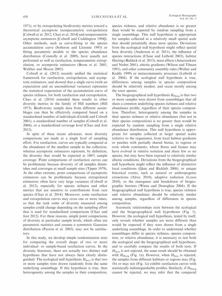
and the biogeographical null hypotheses (Fig. 1).However, the ecological null hypothesis, tested by itself,only reveals whether samples are more different thanwould be expected if they were drawn from a singleunderlying assemblage. In order to understand whetherassemblages differ in species richness, species composi-tion, or relative abundance, it is necessary to test boththe ecological and the biogeographical null hypotheses,and to carefully compare the results of both tests. IfH0eco is not rejected, the same result should be obtainedwith H0biog (Fig. 1a). However, when H0eco is rejected,the samples from different habitats or regions may (Fig.1b) or may not (Fig. 1c) exhibit rarefaction curves withstatistically indistinguishable profiles. Similarly, if H0biog

cannot be rejected, we may infer that the compared

LUIS CAYUELA ET AL.438 Ecological MonographsVol. 85, No. 3

samples are similar regarding richness and relativeabundance, regardless of whether they share most(Fig. 1a), few, or no (Fig. 1b) species, but samples forwhich the biogeographic null hypothesis is rejected willalso, necessarily, appear nonrandom when compared tothe ecological null hypothesis (Fig. 1c). For examples,biotas from tropical rainforests of Africa and Asia mightdiffer completely in species composition (few or noshared species), but might exhibit similar speciesrichness and species relative abundance because ofconstraints imposed by similar climates. If so, samplesfrom the two continents would reject H0eco, but mightnot reject H0biog. If both null hypotheses are rejected,then the assemblages differ in species composition, aswell as in species richness and relative abundance.In this study, we developed randomization algorithms

to test both the ecological and the biogeographical nullhypotheses with sample- or individual-based ecologicaldata. This broadens the scope of rarefaction curves totest relevant null hypotheses regarding communitystructure. If sample sizes are equal, our results may besimilar to those obtained with multivariate approaches,such as distance-based dissimilarity measurements(Legendre and Gallagher 2001, Clarke et al. 2006, DeCaceres et al. 2013). However, it is often the case thatcomparisons are desired for data that are unequallysampled, in which case randomization tests based onrarefaction may offer some distinct advantages.To evaluate the performance of these algorithms and

their vulnerability to Type I or Type II statistical error,we applied them to a series of artificial benchmark datasets that were either drawn from the same assemblage,or drawn from multiple assemblages that differedsystematically in their species composition, richness, orrelative abundance distributions. Finally, we illustrated

the use of these methods in an analysis of forest tree datafrom six 20–52-ha plots in tropical regions around theworld, and to a smaller-scale transect survey of trees inmontane cloud forests sampled in three regions ofChiapas, southern Mexico.

METHODS

Notation and organization of biodiversity data

Following Colwell et al. (2012) and Gotelli and Chao(2013), we use a common set of notation to describebiodiversity sampling data. Consider a complete assem-blage for which all species and their relative abundancesare known. In this complete assemblage, there are i¼ 1to S species and N* total individuals, with Ni individualsof species i. For individual-based (abundance) data, thereference sample consists of n individuals drawn atrandom from N*, with Sobs species present, eachrepresented by Xi individuals. Individual-based datacan be represented as a single vector of length Sobs, theelements of which are the observed abundances Xi.

For sample-based incidence data, the reference sampleconsists of a set of T standardized sampling units, suchas traps, plots, transect lines, etc. Within each of thesesampling units, the presence (1) or absence (0) of eachspecies are the required data, even though abundancedata may have been collected. Sample-based incidencedata can be represented as a single matrix, with i¼ 1 toSobs rows and j¼ 1 to T columns, and entries Wij¼ 1 orWij¼ 0 to indicate the presence or absence of species i insampling unit j.

In this study, we made extensive use of rarefactioncurves for both individual- and sample-based data. Inthe past, rarefaction curves have been estimated byrepeated subsampling, but it is no longer necessary.

FIG. 1. Relationships between the ecological (H0eco) and the biogeographical (H0biog) null hypotheses. Note that the H0eco

encompasses three properties of ecological communities: species composition, richness, and relative abundance (outer circle),whereas the H0biog only comprises two out of these three properties, namely species richness and relative abundance (inner shadedcircle). (a) If two or more samples are drawn from the same assemblage, their species composition, richness, and relative abundancewill be similar, and both the H0eco and the H0biog will be accepted. (b) If samples are drawn from two assemblages with similarspecies richness and relative abundance but different species composition, the H0eco will be rejected, whereas the H0biog will not. (c)If samples are drawn from two assemblages with different species composition and either different species richness, relativeabundance, or both, then both H0eco and the H0biog will be rejected.

August 2015 439NULL MODEL TESTS FOR RAREFACTION CURVES

Instead, we used analytical expressions for rarefactioncurves recently consolidated from previous work ornewly derived by Chao et al. (2014). For each referencesample (or pseudosample), equations from Tables 1 and2 of Chao et al. (2014) were used to generate,analytically, the expected diversity and sample coveragefor each level of subsampling (Appendix A).

Rarefaction curves and diversity indices

We present results for standard rarefaction curves, inwhich the x-axis is either the abundance (individual-based) or number of samples (sample-based). Inaddition, we also carried out all analyses using theestimated coverage of either abundance or number ofsamples as the x-axis in the sampling curve (Chao andJost 2012). Coverage is defined as the proportion of totalindividuals or samples from the complete assemblagethat is represented by the species present in the sampleor subset of samples. Rescaling the data to estimatedcoverage may provide a more powerful comparison ofrarefaction curves (Chao and Jost 2012). Coverageanalyses were conducted for both individual- andsample-based rarefaction.We present results for all tests using species richness as

the diversity index. Although species richness is the mostpopular diversity index, it is quite sensitive to samplesize (Gotelli and Colwell 2001), and does not incorpo-rate information on species abundances. Species rich-ness, itself, is part of a mathematical series of diversityindices known as Hill numbers (Hill 1973), which can bealgebraically transformed into familiar diversity indices,but have better statistical properties (Chao et al. 2014).The order q of the Hill number determines the weightinggiven to more common species, with species richnessdefined by q ¼ 0. In the supplementary material(Appendix B), we present results of parallel tests forall analyses of Hill numbers q¼ 1 (exponential Shannonindex), and q ¼ 2 (the ‘‘inverse’’ Simpson index).All of the tests described have been implemented in

the accompanying ‘‘rareNMtests’’ package (Supplement;Cayuela and Gotelli 2014) for R (R Development CoreTeam 2013).

Ecological null hypothesis

In early studies on rarefaction, the original nullhypothesis was that species richness in a small collection(a subsample of a specified size) could be viewed as arandom subset of a larger collection (the referencesample; Simberloff 1979). However, the null hypothesisthat ecologists usually want to ask is whether two ormore reference samples (or subsamples of them) couldbe viewed as random draws from a single assemblage(Gotelli and Colwell 2011). This comparison is morechallenging because it requires some estimate of theunconditional variance associated with sampling fromthe true assemblage (Colwell et al. 2004), rather thanjust the conditional variance associated with subsam-pling from the largest sample in the collection.

In this study, the ecological null hypothesis H0eco isthat two (or more) reference samples, represented byeither abundance or incidence data, were both drawnfrom the same assemblage of N* individuals and Sspecies. Therefore, any differences among the samples inspecies composition, species richness, or relative abun-dance reflect only random variation, given the numberof individuals (or sampling units) in each collection. Thealternative hypothesis, in the event that H0eco cannot berejected, is that the sample data were drawn fromdifferent assemblages. If H0eco is true, then pooling thesamples should give a composite sample that is also a(larger) random subset of the complete assemblage. It isfrom this pooled composite sample that we makerandom draws for comparison with the actual data.

EcoTest metric

We begin by plotting the expected rarefaction curvesfor the individual samples (Fig. 2a) and for the pooledcomposite sample (Fig. 2b). Next, for each individualsample i, we calculate the cumulative area Ai betweenthe sample rarefaction curve and the pooled rarefactioncurve (Fig. 2c). For a set of i¼ 1 to K samples, we definethe observed difference index

Zobs ¼XK

i¼1

Ai:

Note that two identically shaped rarefaction curvesmay nevertheless differ from the curve for the pooledsample. This difference can arise because speciesidentities in the individual samples are retained in thepooled composite sample, which affects the shape of thepooled rarefaction curve. See Crist and Veech (2006) fora similar approach to partitioning b diversity.

EcoTest randomization algorithm

The data are next reshuffled by randomly reassigningevery individual to a reference sample (for abundancedata) or every sampling unit to a reference sample (forincidence data), and preserving the original sample sizes(number of individuals for abundance data, and numberof sample units for incidence data). From this random-ization, we again construct rarefaction curves andcalculate Zsim (Fig. 2d) as the cumulative area betweenthe rarefaction curves of the randomized samples andthe composite rarefaction curve. This procedure isrepeated many times, leading to a distribution of Zsim

values and a 95% confidence interval (Fig. 1e). Theposition of Zobs in the tail of this distribution is used asan estimate of the probability to randomly obtain thisvalue given the null distribution of the cumulative areabetween the rarefaction curves of the randomizedsamples and the composite rarefaction curve, i.e.,p(Zobs jH0eco). Large values of Zobs relative to the nulldistribution imply that observed differences amongsamples in species composition, richness, and/or relative


abundance are improbable if the samples were all drawn

from the same assemblage.

Biogeographical null hypothesis

In a discussion of the properties of rarefaction curves,

Simberloff (1979) noted that differences in species

composition can obviously lead to rejection of H0eco,

even if the rarefaction curves have similar profiles: ‘‘But

since rarefaction uses only the species-individuals’

distributions, and not the species’ names, it makes little

sense to rarefy a large sample to compare it to some

smaller sample if the species in the two samples are very

different. If a large sample consists primarily of

butterflies and a smaller one is mostly moths, we do

not need rarefaction to tell us that the smaller could not

reasonably be viewed as a random draw from the

larger . . .’’

For this reason, one of the stated assumptions of

traditional rarefaction was that the species lists being

compared are ‘‘taxonomically similar’’ (Tipper 1979,

Gotelli 2008). But in many biogeographic comparisons,

it is already known that the species composition is

different, yet we wish to assess whether two or more

reference samples differ in richness or other measures of

diversity. The question of interest is not ‘‘were two or

more samples randomly drawn from the same underlying

species assemblage?’’ but ‘‘does species richness (or any

other diversity metric) differ among reference samples

FIG. 2. Schematic representation of the EcoTest metric and algorithm: (a) rarefaction curves for the individual samples; (b)rarefaction curve of the pooled composite sample; (c) test statistic Zobs is calculated as the cumulative area Ai between eachindividual sample rarefaction curve and the pooled rarefaction curve; (d) data are reshuffled by randomly reassigning everyindividual to a reference sample (for abundance data) or every sampling unit to a reference sample (for incidence data), whilepreserving the original sample sizes (number of individuals for abundance data and number of sample units for incidence data).From this randomization, we again construct rarefaction curves and calculate Zsim as the cumulative area between the rarefactioncurves of the randomized samples and the composite rarefaction curve; (e) this procedure is repeated many times, leading to adistribution of Zsim values and 95% confidence intervals. The position of Zobs in the tail of this distribution is used as an estimate ofp(Zobs jH0eco). For the purposes of illustration, the composite curve is portrayed as extending only a small distance beyond the tworeference samples. However, in the actual analyses, the x-axis for the composite sample must be the sum of the sampling effort foreach of the reference samples, so it would extend much further to the right. However, the test statistic is only based on the portionof the composite curve that overlaps with the rarefaction curves of the individual samples. The tables are included solely as visualaids; all data presented is completely arbitrary.


after adjusting for differences in abundance or samplingeffort?’’ The biogeographical null hypothesis (H0biog) isthat, regardless of differences in species composition, theprofiles of two or more rarefaction curves are similarenough that they might have been drawn from assem-blages that do not differ significantly in richness or inunderlying species abundance distribution.

BiogTest metric

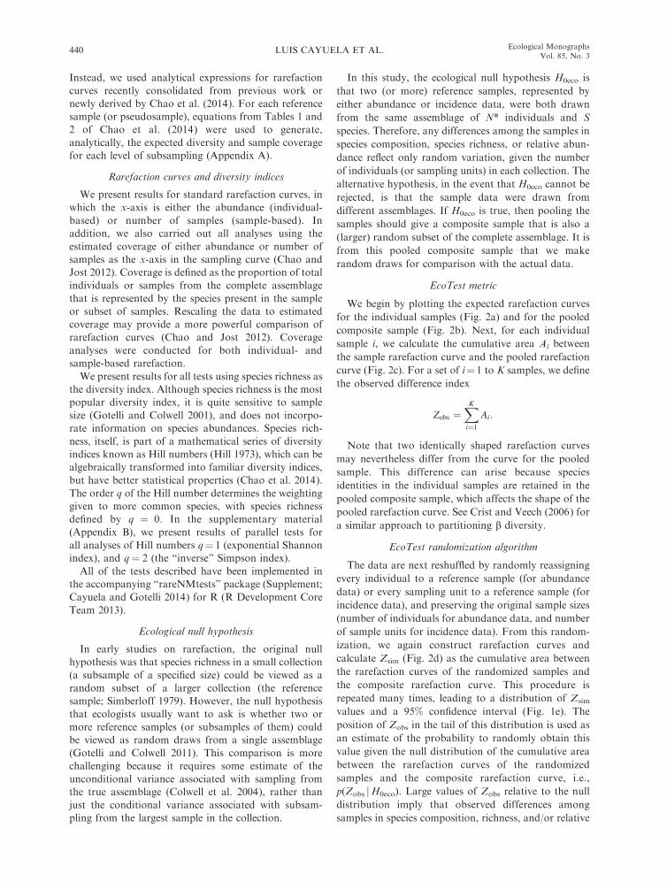
We were not able to devise a BiogTest based on acomposite sample that was strictly analogous to theEcoTest. Instead, we constructed both a different metricand a different algorithm to test H0biog. To do so, wefirst calculated as a test statistic the summed areabetween all unique pairs ab of the K sample rarefactioncurves (Fig. 3a, b)

Zobs ¼XK

a¼1;b¼1

Aab:

If H0biog is true, then Zobs should be relatively smallbecause all of the rarefaction curves should have similarprofiles, regardless of their species composition. In thelimit, if all of the rarefaction curves had an identicalprofile, Zobs would equal 0.

BiogTest randomization algorithm

To construct the null distribution, we created randomassemblages by sampling from a presumed underlyingspecies abundance distribution. Of the many possibledistributions, including the log-series, log-normal, andbroken stick, which distribution should be used? For ourpurposes, the log-normal distribution has some advan-

FIG. 3. Schematic representation of the BiogTest metric and algorithm: (a) expected rarefaction curves for the individualsamples; (b) test statistic Zobs is calculated as the cumulative area between all unique pairs ab of K sample rarefaction curves; (c) thenull distribution is constructed by creating random assemblages from a family of log-normal abundance distributions. Theparameters of each of these distributions were set to specify a suite of distributions that might act as a reasonable samplinguniverse. Random samples are then drawn from each of the simulated assemblages, and Zsim is calculated as the cumulative areabetween all K unique pairs ab of the randomized sample rarefaction curves; (d) this procedure is repeated many times, leading to adistribution of Zsim values and a 95% confidence interval. The position of Zobs in the tail of this distribution is used as an estimateof p(Zobs jH0biog). The tables are included solely as visual aids; all data presented is completely arbitrary.


tages: (1) for some parameter values, the log-normalgenerates a typical right-skewed distribution (many rarespecies, and a few common species) typical of well-sampled assemblages (Preston 1962a, b), (2) abundanceand occurrence data collected for many taxa at widelydifferent spatial scales often conform to an approximatelog-normal distribution (Ulrich et al. 2010), (3) log-normal distributions approximate the species abundancedistribution of important mechanistic models, includingthe neutral model (McGill et al. 2006) and stochasticversions of some niche partitioning models (Tokeshi1993), and (4) depending on the underlying parametervalues and the sample sizes, the log-normal can alsogenerate species abundance profiles that resemble a logseries or geometric series of abundances (Wilson 1993,McGill et al. 2007). Whether the log-normal distributionitself is caused by species interactions or reflects neutralprocesses or sampling intensity is still open to debate(McGill 2003, Sugihara et al. 2003), but is immaterial forour purposes here.The statistical parameters of the log-normal rank

abundance distribution are the number of species in theassemblage and the variance of the distribution; thelatter controls the differences in abundance betweencommon and rare species. If these underlying parame-ters are known, then sample size effects can be estimatedby random sampling of individuals from the specifieddistribution. However, it is very difficult to directlyestimate these parameters from a sample or set ofsamples (O’Hara 2005). Instead, we generated a suite oflog-normal distributions that, taken together, might actas a reasonable sampling universe for comparison with aset of reference samples to test the biogeographic nullhypothesis. Our strategy was to specify a distribution foreach of the two parameters in the log-normal: speciesnumber and variance. As in a random-effects model(Zuur et al. 2009), each replicate of the null distributionreflects a single sample from a log-normal distribution inwhich the two model parameters were first determinedby random assignment.For the lower boundary of species richness, the

minimum possible value cannot be smaller than themaximum number of species observed in the richestsingle sample among a set of samples. For the upperboundary of species richness, we calculated the upperbound of the Chao1 95% confidence interval (Chao1984) for asymptotic species richness of each sample.The number of species in each null assemblage was thenset as a random draw from a uniform distributionbounded at the low end by the maximum observed S andbounded at the high end by the maximum upper boundof the Chao1 95% confidence interval.For the standard deviation of the log-normal, we

sampled a random uniform value between 1.1 and 33(0.1 and 3.5 on a natural logarithm [henceforth referredto as ln] scale). For empirical assemblages, standarddeviations typically fall within this range (Limpert et al.2001). Once the null assemblage was specified by

selection of parameters for species richness and thestandard deviation, we sampled (with replacement) thespecified number of individuals for each sample in anindividual-based data set (Fig. 3c). For incidence data,we sampled (without replacement) the observed numberof species in each sampling unit (i.e., total number ofincidences), with sample probabilities set proportionalto relative abundances in the log-normal distribution.For example, if 15 species were observed in one samplingunit, the equivalent sampling unit in the simulated dataset should also contain 15 species, though not necessar-ily the same ones. We then used the analytic formulas inChao et al. (2014) to construct the rarefaction curves foreach of the pseudosamples. The analysis from this pointforward is the same as for the EcoTest. Namely, wegenerated a distribution of Zsim and compared it to Zobs

to estimate p(Zobs jH0biog) (Fig. 3d).The BiogTest can be used for other species abundance

distributions (other than the log-normal) to constructthe null distribution test, namely the broken stick andgeometric series distributions. We used the broken stickbecause it is the most even of all species abundancedistributions, whereas the geometric series can generatehighly uneven distributions (Magurran 2003). For thebroken stick, the number of species in the assemblagemust first be known, then a random partition is made todefine the relative abundance of each species. For thegeometric series, two parameters are needed: the numberof species in the assemblage and a constant ratio D (D ,1), which determines the abundance of the next speciesin the sequence. In the geometric series, D was obtainedby sampling a random uniform value between 0.1 and 1.In all cases, the number of species (S ), as in the log-normal distribution, was obtained by randomly drawingfrom a uniform distribution that was bounded at the lowend by the maximum observed S and at the high end bythe maximum upper bound of the 95% confidenceinterval for Chao1.

To better mimic the sampling process, a negativebinomial random error was added to the abundancecounts every time a sample was randomly drawn fromthe simulated assemblage. The negative binomialdistribution was used to generate realistic heterogene-ity that often results from spatial clustering ofindividuals and other small-scale processes (Greenand Plotkin 2007, Bolker 2008). The expectation l ofthe negative binomial was represented by the abun-dance count of each species in the assemblage (seeexample in the Supplement). The variance of thenegative binomial is

var ¼ lþ l2

k

where k is the dispersion parameter. For every species,k was randomly drawn from a uniform distributionbetween 0.01 and 25 each time a sample was drawnfrom the assemblage.


Evaluation of the algorithms

Before a new randomization method is applied toempirical data, its performance needs to be evaluatedwith artificial data sets that have specified characteristics(Gotelli and Ulrich 2012). Two properties are desirablefor our statistical tests of differences in rarefactioncurves. First, when the tests are confronted with samplesthat are drawn from the same assemblage, they shouldnot reject the null hypothesis too frequently; we apply atraditional Type I error (a) criterion of 5%. Second,when these tests are confronted with samples drawnfrom assemblages that differ in species composition,richness, or relative abundance, they should not acceptthe null hypothesis too frequently, that is, the probabil-ity of committing a Type II error (b) should be low.There is no accepted standard for the level of power of atest (1 $ b), but a value of 0.8 (the null hypothesis iscorrectly rejected 80% of the time) has been suggested(Cohen 1992). However, power analysis is rarelyconducted in ecological studies (Toft and Shea 1983),because in most cases it requires specification of analternative hypothesis and an effect size that can bedetected by the test. In this case, the alternative isspecified: samples were drawn from multiple assemblag-es. We do not explicitly define an effect size, but that sizeis determined by the expected area difference (Z ) amongrarefaction curves derived from assemblages that weredefined by random parameter values (as specified earlier)for the log-normal distribution.

Simulation scenarios and benchmark tests

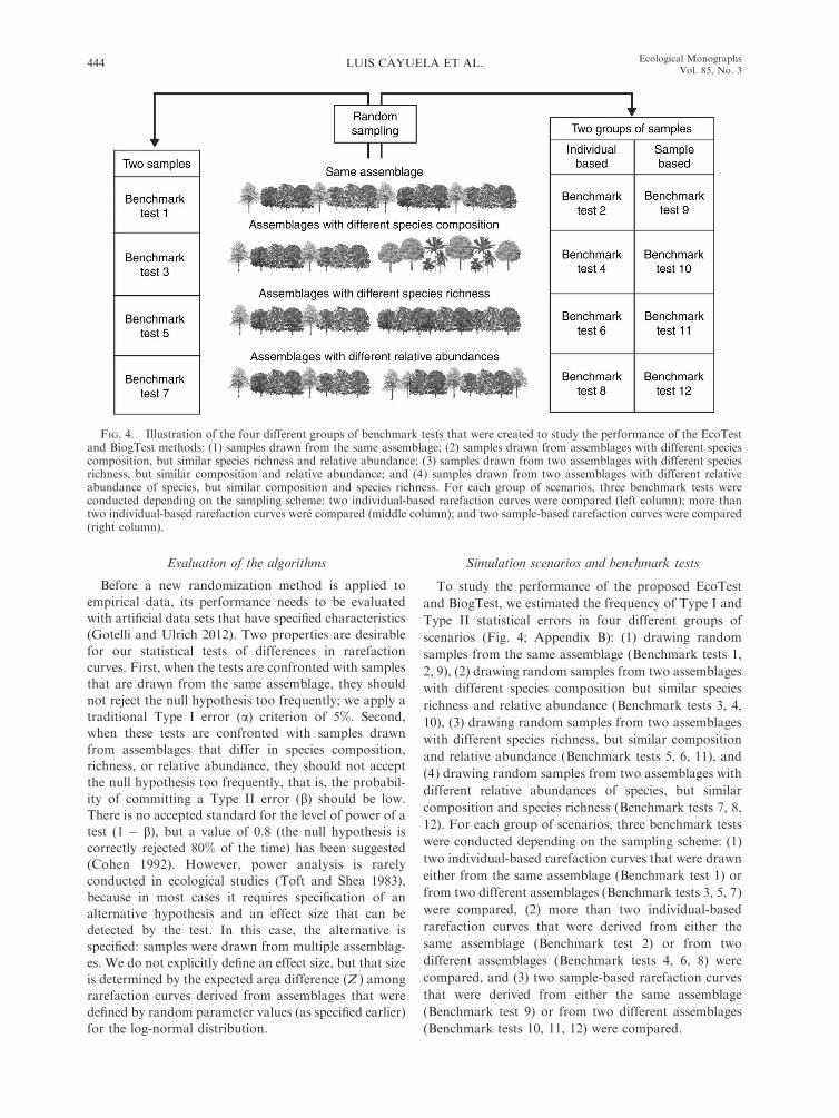
To study the performance of the proposed EcoTestand BiogTest, we estimated the frequency of Type I andType II statistical errors in four different groups ofscenarios (Fig. 4; Appendix B): (1) drawing randomsamples from the same assemblage (Benchmark tests 1,2, 9), (2) drawing random samples from two assemblageswith different species composition but similar speciesrichness and relative abundance (Benchmark tests 3, 4,10), (3) drawing random samples from two assemblageswith different species richness, but similar compositionand relative abundance (Benchmark tests 5, 6, 11), and(4) drawing random samples from two assemblages withdifferent relative abundances of species, but similarcomposition and species richness (Benchmark tests 7, 8,12). For each group of scenarios, three benchmark testswere conducted depending on the sampling scheme: (1)two individual-based rarefaction curves that were drawneither from the same assemblage (Benchmark test 1) orfrom two different assemblages (Benchmark tests 3, 5, 7)were compared, (2) more than two individual-basedrarefaction curves that were derived from either thesame assemblage (Benchmark test 2) or from twodifferent assemblages (Benchmark tests 4, 6, 8) werecompared, and (3) two sample-based rarefaction curvesthat were derived from either the same assemblage(Benchmark test 9) or from two different assemblages(Benchmark tests 10, 11, 12) were compared.

FIG. 4. Illustration of the four different groups of benchmark tests that were created to study the performance of the EcoTestand BiogTest methods: (1) samples drawn from the same assemblage; (2) samples drawn from assemblages with different speciescomposition, but similar species richness and relative abundance; (3) samples drawn from two assemblages with different speciesrichness, but similar composition and relative abundance; and (4) samples drawn from two assemblages with different relativeabundance of species, but similar composition and species richness. For each group of scenarios, three benchmark tests wereconducted depending on the sampling scheme: two individual-based rarefaction curves were compared (left column); more thantwo individual-based rarefaction curves were compared (middle column); and two sample-based rarefaction curves were compared(right column).


We created sets of artificial data matrices for eachscenario and sampling scheme, for which carefullyselected, contrasting parameter combinations were used(Table 1). For those tests in which no rejection of thenull hypothesis was expected, we estimated the proba-bility of incorrectly rejecting H0 as the proportion ofmatrices for which P values were below the standard0.05 threshold, based on 200 randomizations of eachmatrix (i.e., Type I error). For those tests in whichrejection of the null hypothesis was expected, weestimated the probability of incorrectly failing to rejectH0 as the proportion of matrices for which P values wereabove the standard 0.05 threshold, based on 200randomizations of each matrix (i.e., Type II error).Although it is common to use 1000 or more random-izations in null model tests (Manly 2006), we foundconsistent results with 200 randomizations.Parameters of the simulated artificial assemblages

such as the mean species richness or evenness (measuredas the standard deviation of the log-normal) were fixedin some scenarios, but in others were allowed to varyrandomly among the artificial matrices (Table 1). Fixedvalues of richness of 50 and 150 species were used for

Scenarios 5, 6, and 11, which were designed to test fordifferences in species richness. Note that these speciesrichness levels refer to the assemblage from which thesamples were drawn. Differences in species richnessamong the sampled matrices (which have fewer individ-uals or samples than the entire assemblage) were muchsmaller, with an average difference between pairs ofsamples of 43.7 species and a 95% confidence interval of3–96 species. In other scenarios, species richness variedwithin each matrix, and was selected randomly fromwithin a uniform range of 10–200 species. A fixeddifference of the standard deviation of one unit on a lnscale was used for Scenarios 7, 8, and 12, which weredesigned to test for differences in the rank abundancedistribution. In all other scenarios, the standarddeviation of the log-normal did not vary among theassemblages, and was chosen randomly from a uniformrange of 0.1–3.5 on a ln scale (values based on Limpertet al. [2001]).

The extent of sampling was also allowed to varyrandomly to represent realistic sampling differences thatmight be found in typical biodiversity surveys (Table 1).In individual-based scenarios for which only two sites

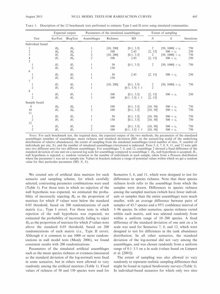
TABLE 1. Description of the 12 benchmark tests performed to estimate Type I and II error using simulated communities.

Test

Expected output Parameters of the simulated assemblages Extent of sampling

IterationsEcoTest BiogTest Assemblages Richness SD N S

Individual based

1 H0 H0 1 [10, 200] [0.1, 3.5] 2 [50, 1000] þ ei 7502 H0 H0 1 100 2.45 [2, 15] 500 þ ei 2503 H1 H0 2 [10, 200] [0.1, 3.5] 2 [50, 1000] þ ei 7504 H1 H0 2 100 2.45 [2, 15] 500 þ ei 25051 H1 H1 1 50 [0.1, 3.5] 2 [50, 1000] þ ei 7502 H1 H1 1 150

61 H1 H1 1 50 2.45 [2, 15] 500 þ ei 2502 H1 H1 1 150

71 H1 H1 1 [10, 200] [0.1, 3.5] 2 [50, 1000] þ ei 7502 H1 H1 1 [0.1, 3.5] 6 1 2

81 H1 H1 1 100 [0.1, 3.5] [2, 15] 500 þ ei 2502 H1 H1 1 100 [0.1, 3.5] 6 1 [2, 15]

Sample based

9 H0 H0 1 100 [0.1, 3.5] [10, 50] 500 þ ei 75010 H1 H0 2 100 [0.1, 3.5] [10, 50] 500 þ ei 750111 H1 H1 1 50 [0.1, 3.5] [10, 50] 500 þ ei 7502 H1 H1 1 150 [0.1, 3.5] [10, 50] 500 þ ei 750

121 H1 H1 2 100 [0.1, 3.5] [10, 50] 500 þ ei 7502 H1 H1 2 100 [0.1, 3.5] 6 1 [10, 50] 500 þ ei 750

Notes: For each benchmark test, the required data, the expected output of the two methods, the parameters of the simulatedassemblages (number of assemblages, mean richness and standard deviation [SD; on the natural-log scale] of the underlyingdistribution of relative abundances), the extent of sampling from the simulated assemblages (total number of sites, N, number ofindividuals per site, S ), and the number of simulated assemblages (iterations) is indicated. Tests 5, 6, 7, 8, 9, 11, and 12 were splitinto two different tests for two different assemblages. For assemblages 7, 8, and 12, assemblage 2 showed a fixed difference of thestandard deviation of one unit on a natural-log scale for assemblage compared to assemblage 1. H0, null hypothesis is accepted;H1,null hypothesis is rejected; ei, random variation in the number of individuals in each sample, taken from a Poisson distributionwhere the parameter k was set to sample size. Values in brackets indicate a range of potential values within which we get a randomvalue for that particular parameter (SD, N, S ).


were compared (Scenarios 1, 3, 5, 7), the number ofindividuals per site was chosen randomly between 50and 1000 individuals in each artificial matrix. Inindividual-based scenarios for which more than twosites were compared (Scenarios 2, 4, 6, 8) and forsample-based scenarios (9, 10, 11, 12), the number ofindividuals was set constant at 500 per site. To includesome realistic sampling variation, we added a Poissonerror to the number of individuals in each sample, wherethe parameter k of the Poisson distribution was set tosample size. The number of artificial matrices generatedfor each benchmark test was set at 250 (Scenarios 2, 4, 6,8) or 750 (Scenarios 1, 3, 5, 7, 9–12). In all, 24 variationsof benchmark tests (6 for EcoTest and 18 for BiogTest)were conducted for each artificial matrix to account for(1) individual- or sample-based vs. coverage-basedrarefaction curves, (2) different Hill numbers (q ¼ 0, q

¼ 1, q¼ 2), (3) the use of the EcoTest and BiogTest, and(4) different distributions of null assemblages for theBiogTest (Table 2).In summary, we set up four different groups of

scenarios, with three sampling schemes each, generatedeither 250 or 750 artificial data matrices for eachcombination of scenario and sampling scheme, andapplied 24 benchmark tests (Appendix B). All theanalyses were conducted in R (R Development CoreTeam 2013) and run at the Bioportal server, a web-basedportal for data analysis that allows for parallelprocessing. Computation time for the suite of differentbenchmark tests ranged from two days (for comparisonof sample-based rarefaction curves) to four weeks (forcomparison of multiple individual-based rarefactioncurves). Overall, running all benchmark tests on thedifferent sets of artificial matrices required more thantwo months of processing time at the Bioportal server.However, the analysis of a typical data set on a personalcomputer can be completed in reasonable amounts oftime. For example, on a 64-bit Intel Core laptop with 7.8GB of memory (Intel, Santa Clara, California, USA), acomparison with 200 iterations of two individual-basedrarefaction curves for tropical trees with ;20 000 and15 000 individuals, and 226 and 173 species, respectively,took 30 min for the EcoTest and 19 min for theBiogTest. The R code used to run all benchmark tests isavailable in the Supplement.

Description of case studies

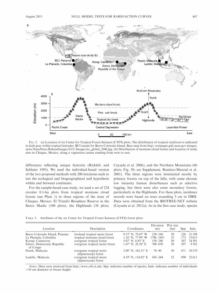
In addition to the benchmark tests with artificial datasets, we also applied the methods to two empirical datasets, one with abundance data (i.e., individual-basedrarefaction curves) and one with incidence data (i.e.,sample-based rarefaction curves). For the individual-based case study, we used tree data from six 20–52-haplots established at several tropical sites around theworld: two plots in South America, two in Africa, andtwo in Southeast Asia (Fig. 5a and Table 3). Species listsand abundances for these plots are available at theCenter for Tropical Forest Sciences (CTFS) website. Wepooled the plot data from each site, and analyzed theabundance of individual trees exceeding 10 cm indiameter at breast height (DBH). The CTFS projectuses the taxonomy of the Angiosperm Phylogeny Groupfor the orders and families of flowering plants (Angio-sperm Phylogeny Group 2009). All species names wereadditionally cross-checked against The Plant List usingthe Taxonstand R package (Cayuela et al. 2012b) toavoid the use of synonyms and to correct typographicalerrors (The Plant List database is available online).6 Wecompared individual-based rarefaction curves for Hillnumbers q ¼ 0 (i.e., species richness), q ¼ 1, and q ¼ 2using either sample size (i.e., number of individuals) orsample coverage. Continental patterns may reflectconstraints imposed by similar climates as well as

TABLE 2. Variations of the ecological and biogeographical nullmodel tests run on simulated matrices in each benchmarktest.

Test type (x-axis),Hill number order (y-axis),

and methodDistribution ofnull assemblages

Individual- or sample-based

q ¼ 0

EcoTest NABiogTest log-normalBiogTest geometricBiogTest broken stick

q ¼ 1

EcoTest NABiogTest log-normalBiogTest geometricBiogTest broken-stick

q ¼ 2


Coverage-based

q ¼ 0


q ¼ 1


q ¼ 2


Note: NA, not applicable. Hill numbers were given differentorders (q); q ¼ 0, (c, d) q ¼ 1, and (e, f ) q ¼ 2; q of the Hillnumber determines the weighting given to more commonspecies, with species richness defined by q ¼ 0, the exponentialShannon index shown by q¼ 1, and the inverse Simpson indexshown by q ¼ 2.

6 http://www.theplantlist.org


differences reflecting unique histories (Ricklefs andSchluter 1993). We used the individual-based versionof the two proposed methods with 200 iterations each totest the ecological and biogeographical null hypothesiswithin and between continents.

For the sample-based case study, we used a set of 224circular 0.1-ha plots from tropical montane cloudforests (see Plate 1) in three regions of the state ofChiapas, Mexico: El Triunfo Biosphere Reserve in theSierra Madre (100 plots), the Highlands (38 plots;

Cayuela et al. 2006), and the Northern Mountains (86plots; Fig. 5b; see Supplement; Ramırez-Marcial et al.2001). The three regions were dominated mostly byprimary forests on top of the hills, with some chroniclow intensity human disturbances such as selectivelogging, but there were also some secondary forests,particularly in the Highlands. For these plots, incidencerecords were based on trees exceeding 5 cm in DBH.Data were obtained from the BIOTREE-NET website(Cayuela et al. 2012a). As in the first case study, species

FIG. 5. (a) Location of six Center for Tropical Forest Sciences (CTFS) plots. The distribution of tropical rainforest is indicatedin dark gray within tropical latitudes. BCI stands for Barro Colorado Island. Base map from http://eoimages.gsfc.nasa.gov/images/news/NasaNews/ReleaseImages/LCC/Images/lcc_global_2048.jpg. (b) Distribution of montane cloud forests and location of studysites in Chiapas, Mexico, along a vegetation catena running from west to east.

TABLE 3. Attributes of the six Center for Tropical Forest Sciences (CTFS) forest plots.

Location Description CoordinatesElevation

(m)Plot size(ha) Spp. Inds.

Barro Colorado Island, Panama lowland tropical moist forest 9.158 N, 79.858 W 120–160 50 226 21 198La Planada, Colombia tropical montane cloud forest 1.168 N, 77.998 W 1796–1891 25 173 15 013Korup, Cameroon evergreen tropical forest 5.078 N, 8.858 E 150–240 50 307 24 591Edoro, Democratic Republicof Congo

evergreen tropical moist forest 1.478 N, 28.588 E 700–850 20 207 9 382

Pasoh, Malaysia evergreen tropical moist(dipterocarp) forest

2.988 N, 102.318 E 70–90 50 671 28 279

Lambir, Malaysia evergreen tropical moist(dipterocarp) forest

4.198 N, 114.028 E 104–244 52 990 32 611

Notes: Data were retrieved from http://www.ctfs.si.edu. Spp. indicates number of species, Inds. indicates number of individuals.10 cm diameter at breast height.


names were standardized and typographical errors werecorrected using The Plant List through the TaxonstandR package (Cayuela et al. 2012b). Distances betweenregions ranged from ;50 km (the Highlands andNorthern Mountains) to ;250 km (Sierra Madre andNorthern Mountains). Despite differences in elevationamong these forests, ;53% of the total species occur intwo or more of the forests. Thus, our null hypothesiswas that the three regions should display similarpatterns of species composition, richness, and relativeabundance of species. We used the sample-basedversion of the two proposed methods with 200iterations each to test the ecological and biogeograph-ical null hypotheses between regions.

RESULTS

Benchmark performance of EcoTest

For species richness (q ¼ 0), the EcoTest had Type Ierrors of ;5% for both individual- (Scenarios 1 and 2)and sample-based rarefaction (Scenario 9). The EcoTestalso had very low Type II errors (always less than 1%),so the null hypothesis was almost always rejected whendata were generated from two different assemblages,and then pooled to generate a null distribution fortesting (Table 4, Benchmark tests 3–8, 10–12).For Hill numbers q ¼ 1 and q ¼ 2, Type I error rates

were slightly higher (Appendix B: parts a and b), but stillranged from only 5% to 9%. Type II errors for Hillnumbers q ¼ 1 and q ¼ 2 were very infrequent (alwaysless than 1%). For coverage-based analyses, Type I errorrates for the EcoTest with Hill numbers q¼ 0, q¼ 1, andq¼2 were between 4% and 14% (Appendix B: parts c–e),somewhat higher than the rates for individual- orsample-based rarefaction curves (Table 4). Type II errorrates for coverage-based analyses were always less than6% for all Hill numbers.

Benchmark performance of BiogTest

The BiogTest creates null assemblages by drawingrandom parameter values (species richness and standarddeviation) to simulate a spectrum of log-normaldistributions of species abundances. It is therefore notsurprising that, for both Type I and Type II error testsfor species richness (q ¼ 0), the BiogTest performs wellwhen the test matrices (which simulate empiricalreference samples) themselves were also drawn from alog-normal distribution (Table 4). In such cases, theerror rates in the different scenarios were less than 9%for Type I error, and less than 12% for Type II error.Similar values for Type I and Type II error rates werefound when the assemblages were drawn from a brokenstick distribution, and then compared to a nulldistribution created from a log-normal (Table 4). Whenthe test matrices were created from a geometric seriesdistribution, Type II error rates for species richnessdecreased as compared to a null distribution createdfrom a log-normal. However, Type I error rates for thegeometric series data sets increased to values between25% and 45% for the various scenarios.For Hill numbers q¼1 and q¼2 (Appendix B: parts a

and b), the best performance for the BiogTest was alsofound for the log-normal and broken stick distributions,with Type I errors ranging between 0% and 8%. Type IIerrors were higher for these distributions and in somecases exceeded 70%. As with species richness (q¼ 0), theworst performance for Type I error occurred whensamples were drawn from a geometric series distribution(Appendix B: parts a and b).Both Type I and Type II error rates for all three Hill

numbers (Appendix B: parts c–e), were usually higherfor coverage-based analyses compared to sample- orindividual-based analyses (Appendix B: parts c–e vs.Table 4).

TABLE 4. Percentage of commission of Type I (incorrect rejection of a true null hypothesis) and Type II error (failure to reject afalse null hypothesis) in 12 different benchmark tests (see Table 1 for a description of these tests) for the two proposed methods(EcoTest, BiogTest).

Benchmarktest

EcoTest

BiogTest

Log-normal Geometric Broken stick

Type Ierror

Type IIerror

Type Ierror

Type IIerror

Type Ierror

Type IIerror

Type Ierror

Type IIerror

1 6.13 5.87 25.47 6.532 7.60 5.20 45.20 5.203 0.00 5.20 22.80 7.334 0.00 2.93 44.35 4.185 0.27 6.67 3.07 6.536 0.00 11.30 2.93 10.047 0.60 5.71 4.07 4.678 0.00 1.67 0.00 1.689 4.80 4.00 30.80 3.8710 0.00 8.67 32.67 10.1311 0.13 6.93 3.20 7.3312 0.00 3.47 1.20 4.00

Note: For the BiogTest method, three different underlying distributions of species relative abundances for the benchmark nullmodel communities were used (log-normal, geometric, broken stick). Cells left blank indicate non-applicable data.


CASE STUDIES

An individual-based comparison of global tropicalrainforests

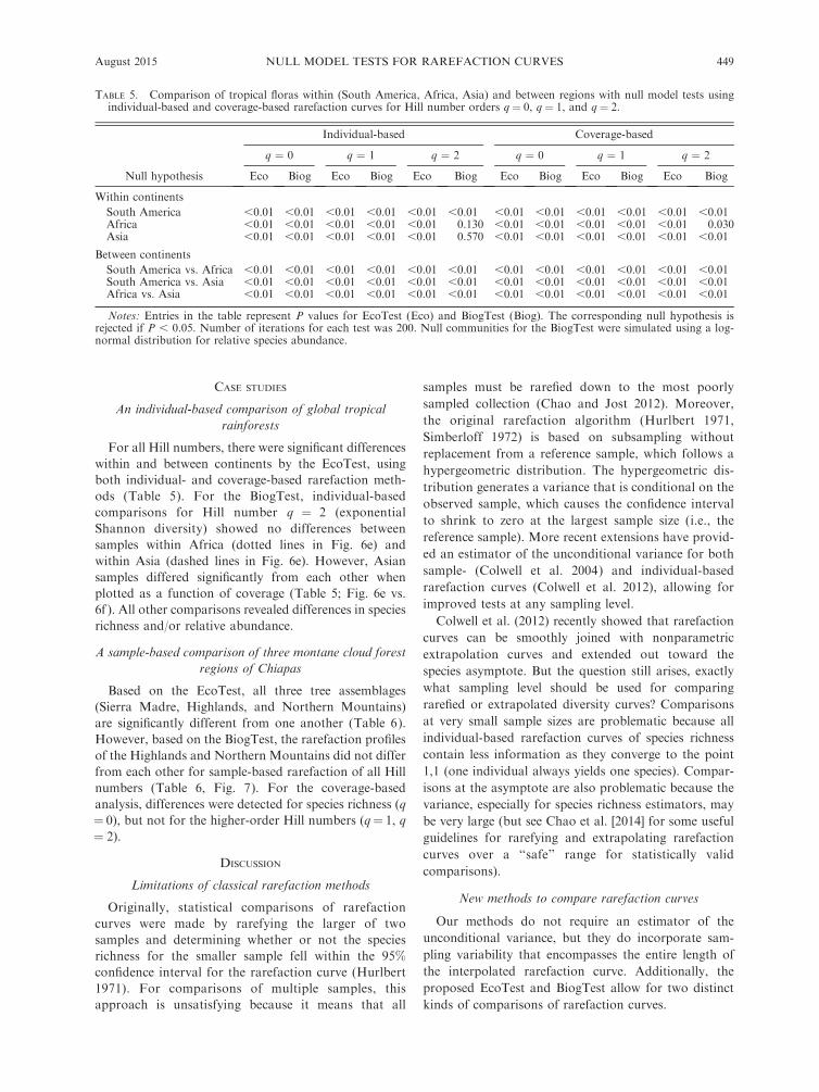
For all Hill numbers, there were significant differenceswithin and between continents by the EcoTest, usingboth individual- and coverage-based rarefaction meth-ods (Table 5). For the BiogTest, individual-basedcomparisons for Hill number q ¼ 2 (exponentialShannon diversity) showed no differences betweensamples within Africa (dotted lines in Fig. 6e) andwithin Asia (dashed lines in Fig. 6e). However, Asiansamples differed significantly from each other whenplotted as a function of coverage (Table 5; Fig. 6e vs.6f ). All other comparisons revealed differences in speciesrichness and/or relative abundance.

A sample-based comparison of three montane cloud forestregions of Chiapas

Based on the EcoTest, all three tree assemblages(Sierra Madre, Highlands, and Northern Mountains)are significantly different from one another (Table 6).However, based on the BiogTest, the rarefaction profilesof the Highlands and Northern Mountains did not differfrom each other for sample-based rarefaction of all Hillnumbers (Table 6, Fig. 7). For the coverage-basedanalysis, differences were detected for species richness (q¼ 0), but not for the higher-order Hill numbers (q¼ 1, q¼ 2).

DISCUSSION

Limitations of classical rarefaction methods

Originally, statistical comparisons of rarefactioncurves were made by rarefying the larger of twosamples and determining whether or not the speciesrichness for the smaller sample fell within the 95%confidence interval for the rarefaction curve (Hurlbert1971). For comparisons of multiple samples, thisapproach is unsatisfying because it means that all

samples must be rarefied down to the most poorlysampled collection (Chao and Jost 2012). Moreover,the original rarefaction algorithm (Hurlbert 1971,Simberloff 1972) is based on subsampling withoutreplacement from a reference sample, which follows ahypergeometric distribution. The hypergeometric dis-tribution generates a variance that is conditional on theobserved sample, which causes the confidence intervalto shrink to zero at the largest sample size (i.e., thereference sample). More recent extensions have provid-ed an estimator of the unconditional variance for bothsample- (Colwell et al. 2004) and individual-basedrarefaction curves (Colwell et al. 2012), allowing forimproved tests at any sampling level.

Colwell et al. (2012) recently showed that rarefactioncurves can be smoothly joined with nonparametricextrapolation curves and extended out toward thespecies asymptote. But the question still arises, exactlywhat sampling level should be used for comparingrarefied or extrapolated diversity curves? Comparisonsat very small sample sizes are problematic because allindividual-based rarefaction curves of species richnesscontain less information as they converge to the point1,1 (one individual always yields one species). Compar-isons at the asymptote are also problematic because thevariance, especially for species richness estimators, maybe very large (but see Chao et al. [2014] for some usefulguidelines for rarefying and extrapolating rarefactioncurves over a ‘‘safe’’ range for statistically validcomparisons).

New methods to compare rarefaction curves

Our methods do not require an estimator of theunconditional variance, but they do incorporate sam-pling variability that encompasses the entire length ofthe interpolated rarefaction curve. Additionally, theproposed EcoTest and BiogTest allow for two distinctkinds of comparisons of rarefaction curves.

TABLE 5. Comparison of tropical floras within (South America, Africa, Asia) and between regions with null model tests usingindividual-based and coverage-based rarefaction curves for Hill number orders q¼ 0, q ¼ 1, and q¼ 2.

Null hypothesis

Individual-based Coverage-based

q ¼ 0 q ¼ 1 q ¼ 2 q ¼ 0 q ¼ 1 q ¼ 2

Eco Biog Eco Biog Eco Biog Eco Biog Eco Biog Eco Biog

Within continents

South America ,0.01 ,0.01 ,0.01 ,0.01 ,0.01 ,0.01 ,0.01 ,0.01 ,0.01 ,0.01 ,0.01 ,0.01Africa ,0.01 ,0.01 ,0.01 ,0.01 ,0.01 0.130 ,0.01 ,0.01 ,0.01 ,0.01 ,0.01 0.030Asia ,0.01 ,0.01 ,0.01 ,0.01 ,0.01 0.570 ,0.01 ,0.01 ,0.01 ,0.01 ,0.01 ,0.01

Between continents

South America vs. Africa ,0.01 ,0.01 ,0.01 ,0.01 ,0.01 ,0.01 ,0.01 ,0.01 ,0.01 ,0.01 ,0.01 ,0.01South America vs. Asia ,0.01 ,0.01 ,0.01 ,0.01 ,0.01 ,0.01 ,0.01 ,0.01 ,0.01 ,0.01 ,0.01 ,0.01Africa vs. Asia ,0.01 ,0.01 ,0.01 ,0.01 ,0.01 ,0.01 ,0.01 ,0.01 ,0.01 ,0.01 ,0.01 ,0.01

Notes: Entries in the table represent P values for EcoTest (Eco) and BiogTest (Biog). The corresponding null hypothesis isrejected if P , 0.05. Number of iterations for each test was 200. Null communities for the BiogTest were simulated using a log-normal distribution for relative species abundance.


The EcoTest addresses the simplest null hypothesis,which is that two samples were drawn from the sameunderlying assemblage, so that any differences in speciesrichness, relative abundance, and species compositionreflect only sampling effects. The EcoTest is a ‘‘distri-bution free’’ test that is based on a pooling of sampledata to generate a null distribution. This test performedvery well in all benchmark comparisons, consistentlydistinguishing samples that were created from distribu-tions that differed in their underlying species richness(Scenarios 5, 6, and 11), relative abundance (Scenarios 7,

8, and 12), or species composition (Scenarios 3, 4, and10; Table 4). The test also had a low Type I error ratewhen data were randomly sampled from a singleunderlying assemblage (Scenarios 1, 2, and 9)

The EcoTest successfully discriminates among sam-ples that differ only in species composition, as expectedaccording to Simberloff (1979). However, it is moreoften the case that multiple samples will contain someshared and some distinct species, as well as undetectedspecies that may also be shared among samples (Chao etal. 2005). Regardless of the similarity of the rarefaction

FIG. 6. Individual- (a, c, e) and coverage-based (b, d, f ) rarefaction curves for the six CTFS forest plots using Hill numbers withweightings (a, b) q¼ 0, (c, d) q¼ 1, and (e, f ) q¼ 2; order q of the Hill number determines the weighting given to more commonspecies, with species richness defined by q¼0, the exponential Shannon index shown by q¼1, and the inverse Simpson index shownby q ¼ 2. Plots from different continents are displayed with different line types: South America with solid lines (Barro ColoradoIsland [black], La Planada [gray]), Africa with dotted lines (Korup [black], Edoro [gray]), and Asia with dashed lines (Lambir[black], Pasoh [gray]). Two hundred iterations were used for each test. Null communities for the BiogTest were simulated using alog-normal distribution for relative species abundance.


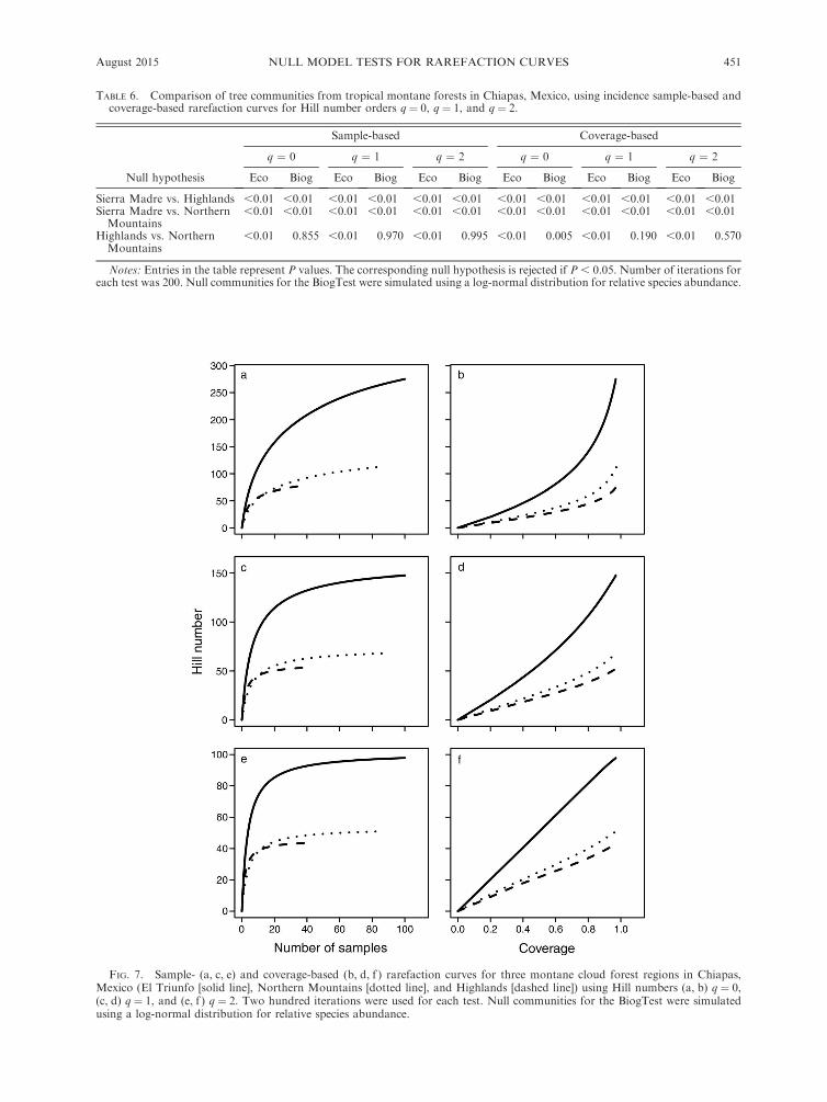
FIG. 7. Sample- (a, c, e) and coverage-based (b, d, f ) rarefaction curves for three montane cloud forest regions in Chiapas,Mexico (El Triunfo [solid line], Northern Mountains [dotted line], and Highlands [dashed line]) using Hill numbers (a, b) q ¼ 0,(c, d) q ¼ 1, and (e, f ) q ¼ 2. Two hundred iterations were used for each test. Null communities for the BiogTest were simulatedusing a log-normal distribution for relative species abundance.

TABLE 6. Comparison of tree communities from tropical montane forests in Chiapas, Mexico, using incidence sample-based andcoverage-based rarefaction curves for Hill number orders q ¼ 0, q ¼ 1, and q ¼ 2.

Null hypothesis

Sample-based Coverage-based

q ¼ 0 q ¼ 1 q ¼ 2 q ¼ 0 q ¼ 1 q ¼ 2

Eco Biog Eco Biog Eco Biog Eco Biog Eco Biog Eco Biog

Sierra Madre vs. Highlands ,0.01 ,0.01 ,0.01 ,0.01 ,0.01 ,0.01 ,0.01 ,0.01 ,0.01 ,0.01 ,0.01 ,0.01Sierra Madre vs. NorthernMountains

,0.01 ,0.01 ,0.01 ,0.01 ,0.01 ,0.01 ,0.01 ,0.01 ,0.01 ,0.01 ,0.01 ,0.01

Highlands vs. NorthernMountains

,0.01 0.855 ,0.01 0.970 ,0.01 0.995 ,0.01 0.005 ,0.01 0.190 ,0.01 0.570

Notes: Entries in the table represent P values. The corresponding null hypothesis is rejected if P , 0.05. Number of iterations foreach test was 200. Null communities for the BiogTest were simulated using a log-normal distribution for relative species abundance.


curves, differences in species composition can lead to astrong rejection of the null hypothesis for the EcoTest(Scenarios 3, 4, and 10). Therefore, it is not surprisingthat, for every empirical comparison of global tropicalrainforests (Fig. 6) and regional montane forests (Fig.7), the EcoTest was always strongly rejected (Tables 5,6).Deviations from the null hypothesis for the EcoTest

can reflect everything from small-scale species interac-tions (which can alter relative abundances amongsample plots; Chase and Leibold 2003) to regionaldifferences in beta diversity (which can reflect turnoverin species composition; Wilson and Tilman 1991,Baldeck et al. 2013) to large-scale differences in speciesrichness (which can reflect differences in evolutionaryrates; Qian and Ricklefs 2008). The sampling nullhypothesis that is made explicit with the EcoTest is thestarting point for comparing rarefaction curves. How-ever, so many forces can affect this test that it is perhapsnot surprising that it will be reliably rejected for well-sampled empirical assemblages such as those in Figs. 6and 7.The EcoTest makes use only of the expected diversity

from the rarefaction curve. For species richness, Li andMao (2012) derived a simultaneous confidence band fora species accumulation curve that can be used toevaluate differences between two accumulation curves,similar to what we have done with the cumulative areaof difference between each rarefaction curve and the

composite curve (Fig. 2c). The randomization algorithmfor the EcoTest is identical to the method of Solow(1993), in which all partitions of the data amongdifferent samples are equally likely, and is similar tothe method developed by Collins et al. (2009) tocompare rank occupancy–abundance profiles (ROAPs).In that sense, the EcoTest belongs to a growing class oftests for differences in b diversity among samples (Cristand Veech 2006, Anderson et al. 2011).In the biogeographic realm, the comparison of interest

is the profile of the rarefaction curve, without regard tothe underlying species composition. In biogeographiccomparisons among distinct regions or continents, it isknown at the outset that there are strong differences inspecies composition, so the EcoTest is not assessing theappropriate null hypothesis. For this question, we werenot able to devise an appropriate algorithm based onpooling of samples to generate a composite distributionfor random subsampling. Because the species names inthe individual samples are not retained, there does notseem to be a reliable way to determine the rank order ofeach species in the full, pooled assemblage. For thisreason, we used a family of log-normal distributions, inwhich the null assemblages were determined fromrandomly chosen parameters for species richness andthe standard deviation, the two underlying parametersof the log-normal.It has long been recognized that both parameter

estimation and the goodness of fit of empirical rank

PLATE 1. Tropical montane forests represent one of the world’s richest repositories of plant biodiversity, and play an importantrole in the provision of regulatory services such as water interception. Photo credit: L. Cayuela.


abundance data are very sensitive to the choice of theunderlying statistical distribution that is used (O’Hara2005, McGill et al. 2007). For this reason, we creatednull distribution data sets using log-normal, geometricseries, and broken stick distributions. The BiogTest hadsatisfactory performance in most cases, although errorrates were unacceptably high when the samples weredrawn from a geometric series (Table 4). In retrospect,the poor fit with the geometric series arises because thedominance fraction D was chosen from a uniform rangeof 0 to 1. For most of this range, the resulting rankabundance distributions fall off very steeply, which doesnot fit well with most log-normal distributions or withmost empirical data sets. In contrast, the rank abun-dance profile of a broken stick series is more even, andthe BiogTest with broken stick and log-normal samplesperforms much better than with geometric seriessamples.

Application to case studies

As we anticipated, the same empirical data set cangive different answers when tested with EcoTest vs.BiogTest. For example, with Hill number q¼ 2, the twoMalaysian forest samples (Pasoh and Lambir; dashedlines in Fig. 6) and the two African forest samples(Edoro and Korup; dotted lines in Fig. 6) differ byEcoTest, but not by BiogTest (Table 5). Visually, thesepairs of curves are nearly coincident in the sample-basedrarefaction plots of Fig. 6e, so it is a sensible result thatthe null hypothesis was not rejected by BiogTest in thesecases. These results are reassuring because the samplesizes underlying these comparisons were very large (9382to 32 611 individuals). In such cases, there is a dangerthat H0 might always be rejected when the sample islarge enough, even when effect sizes are very small.When plotted against coverage, however, the Biog-

Test for these same comparisons is statistically signif-icant (Table 5). Coverage-based analyses do notnecessarily give the same results as traditionalsample- or individual-based rarefaction (Chao and Jost2012), as the shapes of species accumulation curves arevery different when plotted against coverage ratherthan sample size. We note that the coverage-basedrarefaction curves for these data did not overlap as didthe individual-based curves (Fig. 6e vs. 6f ), whichcorresponds to the different outcomes of the statisticaltests.For the smaller-scale comparisons of three mountain

assemblages, the sample-based rarefaction curves for theNorthern Mountains and the Highlands overlappedclosely (Fig. 7a, c, e), and did not differ by the BiogTestfor any of the Hill numbers (Table 6). For the coverage-based analyses, the rarefaction curves again diverged,although only the curves for species richness (Hillnumber q ¼ 0) were statistically significant (Fig.7b, d, f; Table 6). This result is not entirely unexpectedbecause the Sierra Madre and the Chiapas Massif(which includes the Highlands and Northern Moun-

tains) have a different geological history, and wereisolated altitudinally by the Central Depression (Fig. 7b)from the Late Jurassic to the Late Cretaceous (Padilla ySanchez 2007). In addition, the two areas have differenthistories of land use, with the Highlands and NorthernMountains experiencing stronger human impacts fromhunting, logging, and agriculture (Ramırez-Marcial etal. 2001, Cayuela et al. 2006) than the Sierra Madre (N.Ramırez-Marcial, personal communication).

Further prospects

We have presented these analyses in terms of familiardiversity metrics of species richness and higher-order Hillnumbers. However, the same approach could be usedwith any other diversity metric, including univariatemeasures of trait, functional, and phylogenetic diversity.The Chao et al. (2014) procedures could also be used toimprove our tests, but they require asymptotic estima-tors of the diversity metric and its variance, and those areso far available only for Hill numbers (including speciesrichness). Our tests can be applied to any diversity metricthat can be calculated for a reference sample and forbootstrapped random subsamples.

In spite of a long history of use of rarefaction methodsin ecology and evolution, new statistical developmentscontinue to improve the estimation of biodiversitypatterns and statistical inference from sample data.The distinction between the ecological and biogeograph-ic null hypotheses may prove useful in pinpointing howdifferences in species composition, relative abundance,and species richness contribute to biodiversity patterns.

ACKNOWLEDGMENTS

This study was possible thanks to a mobility grant of theSpanish Ministry of Education to L. Cayuela (Jose deCastillejos Programme, CAS 12/00140), and partial fundingby project CGL2013-45634-P. N. J. Gotelli was supported byU.S. NSF DEB 1257625, NSF DEB 1144055, 2, and NSF DEB1136644. R. K. Colwell was supported by Ciencia semFronteiras fellowship (Brazil). Mario Gonzalez- Espinosa andNeptalı Ramırez-Marcial provided part of the plot data for theChiapas data set and valuable comments on the interpretationof the results for this case study. We thank Anne Chao forcomments on the manuscript and for extended correspondenceon rarefaction and asymptotic diversity estimators. We areindebted to the BioPortal for enabling data analyses in theirweb-based portal. Note that the BioPortal no longer exists, as ithas now become the LifePortal. L. Cayuela, N. J. Gotelli, andR. K. Colwell contributed equally to this paper.

LITERATURE CITED

Alroy, J. 2010. The shifting balance of diversity among majormarine animal groups. Science 329:1191–1194.

Amarasekare, P., and R. M. Nisbet. 2001. Spatial heterogene-ity, source–sink dynamics, and the local coexistence ofcompeting species. American Naturalist 158:572–584.

Anderson, M. J., et al. 2011. Navigating the multiple meaningsof b diversity: a roadmap for the practicing ecologist.Ecology Letters 14:19–28.

Angiosperm Phylogeny Group. 2009. An update of theAngiosperm Phylogeny Group classification for the ordersand families of flowering plants: APG III. Botanical Journalof the Linnean Society 161:105–121.


Baldeck, C. A., et al. 2013. Habitat filtering across tree lifestages in tropical forest communities. Proceedings of theRoyal Society B 280:20130548.

Bolker, B. M. 2008. Ecological models and data in R. PrincetonUniversity Press, Princeton, New Jersey, USA.

Brose, U., N. D. Martinez, and R. J. Williams. 2003.Estimating species richness: sensitivity to sample coverageand insensitivity to spatial patterns. Ecology 84:2364–2377.

Cayuela, L., et al. 2012a. The Tree Biodiversity Network(BIOTREE-NET): prospects for biodiversity research andconservation in the tropics. Biodiversity and Ecology 4:211–224.

Cayuela, L., J. D. Golicher, J. M. Rey-Benayas, M. Gonzalez-Espinosa, and N. Ramırez-Marcial. 2006. Effects of frag-mentation and disturbance on tree diversity in tropicalmontane forests. Journal of Applied Ecology 43:1172–1182.

Cayuela, L., and N. J. Gotelli. 2014. rareNMtests: ecologicaland biogeographical null model tests for comparing rarefac-tion curves. R package version 1.0. http://cran.r-project.org/package¼rareNMtests

Cayuela, L., I. Granzow de la Cerda, F. S. Albuquerque, andJ. D. Golicher. 2012b. Taxonstand: an R package for speciesnames standardisation in vegetation databases. Methods inEcology and Evolution 3(6):1078–1083.

Chao, A. 1984. Nonparametric estimation of the number ofclasses in a population. Scandinavian Journal of Statistics11:265–270.

Chao, A., R. L. Chazdon, R. K. Colwell, and T. J. Shen. 2005.A new statistical approach for assessing compositionalsimilarity based on incidence and abundance data. EcologyLetters 8:148–159.

Chao, A., C. H. Chiu, and L. Jost. 2010. Phylogenetic diversitymeasures based on Hill numbers. Philosophical Transactionsof the Royal Society B 365:3599–3609.

Chao, A., R. K. Colwell, C. W. Lin, and N. J. Gotelli. 2009.Sufficient sampling for asymptotic minimum species richnessestimators. Ecology 90:1125–1133.

Chao, A., N. J. Gotelli, T. C. Hsieh, E. L. Sander, K. H. Ma,R. K. Colwell, and A. M. Ellison. 2014. Rarefaction andextrapolation with Hill numbers: a framework for samplingand estimation in species diversity studies. EcologicalMonographs 84:45–67.

Chao, A., and L. Jost. 2012. Coverage-based rarefaction andextrapolation: standardizing samples by completeness ratherthan size. Ecology 93:2533–2547.

Chase, J. M., and M. A. Leibold. 2003. Ecological niches:linking classical and contemporary approaches. University ofChicago Press, Chicago, Illinois, USA.

Clarke, K. R., P. J. Somerfield, and M. G. Chapman. 2006. Onresemblance measures for ecological studies, includingtaxonomic dissimilarities and a zero-adjusted Bray-Curtiscoefficient for denuded assemblages. Journal of ExperimentalMarine Biology and Ecology 330:55–80.

Coddington, J. A., I. Agnarsson, J. A. Miller, M. Kuntner, andG. Hormiga. 2009. Undersampling bias: the null hypothesisfor singleton species in tropical arthropod surveys. Journal ofAnimal Ecology 78:573–584.

Cohen, J. 1992. A power primer. Psychological Bulletin112:155–159.

Collins, C. D., R. D. Holt, and B. L. Foster. 2009. Patch sizeeffects on plant species decline in an experimentallyfragmented landscape. Ecology 90:2577–2588.

Colwell, R. K., A. Chao, N. J. Gotelli, S. Y. Lin, C. X. Mao,R. L. Chazdon, and J. T. Longino. 2012. Models andestimators linking individual-based and sample-based rare-faction, extrapolation, and comparison of assemblages.Journal of Plant Ecology 5:3–21.

Colwell, R. K., and J. A. Coddington. 1994. Estimatingterrestrial biodiversity through extrapolation. PhilosophicalTransactions of the Royal Society B 345:101–118.

Colwell, R. K., C. X. Mao, and J. Chang. 2004. Interpolating,extrapolating, and comparing incidence-based species accu-mulation curves. Ecology 85:2717–2727.

Connolly, S. R., M. Dornelas, D. R. Bellwood, and T. P.Hughes. 2009. Testing species abundance models: a newbootstrap approach applied to Indo-Pacific coral reefs.Ecology 90:3138–3149.

Crist, T. O., and J. A. Veech. 2006. Additive partitioning ofrarefaction curves and species-area relationships: unifyingalpha-, beta- and gamma-diversity with sample size andhabitat area. Ecology Letters 9:923–932.

De Caceres, M., P. Legendre, and F. He. 2013. Dissimilaritymeasurements and the size structure of ecological communi-ties. Methods in Ecology and Evolution 4:1167–1177.

Gotelli, N. J. 2008. A primer of ecology. Fourth edition.Sinauer, Sunderland, Massachusetts, USA.

Gotelli, N. J., and A. Chao. 2013. Measuring and estimatingspecies richness, species diversity, and biotic similarity fromsampling data. Pages 195–211 in S. A. Levin, editor.Encyclopedia of biodiversity. Second edition. Volume 5.Academic Press, Waltham, Massachusetts, USA.

Gotelli, N. J., and R. K. Colwell. 2001. Quantifying biodiver-sity: procedures and pitfalls in the measurement andcomparison of species richness. Ecology Letters 4:379–391.

Gotelli, N. J., and R. K. Colwell. 2011. Estimating speciesrichness. Pages 39–54 in A. E. Magurran and B. J. McGill,editors. Biological diversity: frontiers in measurement andassessment. Oxford University Press, New York, New York,USA.

Gotelli, N. J., A. M. Ellison, and B. A. Ballif. 2012.Environmental proteomics, biodiversity statistics and food-web structure. Trends in Ecology & Evolution 27:436–442.

Gotelli, N. J., and W. Ulrich. 2012. Statistical challenges in nullmodel analysis. Oikos 121:171–180.

Green, J. L., and J. B. Plotkin. 2007. A statistical theory forsampling species abundances. Ecology Letters 10:1037–1045.

Hill, M. O. 1973. Diversity and evenness: a unifying notationand its consequences. Ecology 54:427–432.

Hurlbert, S. H. 1971. The non-concept of species diversity: acritique and alternative parameters. Ecology 52:577–586.

James, F. C., and N. O. Wamer. 1982. Relationships betweentemperate forest bird communities and vegetation structure.Ecology 63:159–171.

Legendre, P., and E. D. Gallagher. 2001. Ecologicallymeaningful transformations for ordination of species data.Oecologia 129:271–280.

Leibold, M. A., et al. 2004. The metacommunity concept: aframework for multi-scale community ecology. EcologyLetters 7:601–613.

Li, J., and C. X. Mao. 2012. Simultaneous confidence inferenceon species accumulation curves. Journal of Agricultural,Biological, and Environmental Statistics 17:1–14.

Limpert, E., W. A. Stahel, and M. Abbt. 2001. Log-normaldistributions across the sciences: keys and clues. BioScience51:341–352.

Losos, J. B. 2010. Adaptive radiation, ecological opportunity,and evolutionary determinism. American Naturalist175:623–639.

Magurran, A. E. 2003. Measuring biological diversity. Wiley-Blackwell, Hoboken, New Jersey, USA.

Magurran, A. E., and B. J. McGill, editors. 2011. Biologicaldiversity: frontiers in measurement and assessment. OxfordUniversity Press, Oxford, UK.

Manly, B. F. J. 2006. Randomization, bootstrap and MonteCarlo methods in Biology. Third edition. Chapman & Hall/CRC Press, Boca Raton, Florida, USA.

McGill, B. J. 2003. Does Mother Nature really prefer rarespecies or are log-left-skewed SADs a sampling artefact?Ecology Letters 6:766–773.

McGill, B. J., et al. 2007. Species abundance distributions:moving beyond single prediction theories to integration


within an ecological framework. Ecology Letters 10:995–1015.

McGill, B. J., B. Maurer, and M. D. Weiser. 2006. Empiricalevaluation of neutral theory. Ecology 87:1411–1423.

O’Hara, R. B. 2005. Species richness estimators: how manyspecies can dance on the head of a pin? Journal of AnimalEcology 74:375–386.

Padilla y Sanchez, R. J. 2007. Evolucion geologica del surestemexicano desde el Mesozoico al presente en el contextoregional del Golfo de Mexico. Boletın de la SociedadGeologica Mexicana 59(1):19–42.

Payton, M. E., M. H. Greenstone, and N. Schenker. 2003.Overlapping confidence intervals or standard intervals? Whatdo they mean in terms of statistical significance? Journal ofInsect Science 3(34):1–6.

Preston, F. W. 1962a. The canonical distribution of common-ness and rarity: part I. Ecology 43:185–215.

Preston, F. W. 1962b. The canonical distribution of common-ness and rarity: part II. Ecology 43:410–432.

Qian, H., and R. E. Ricklefs. 2008. Global concordance indiversity patterns of vascular plants and terrestrial verte-brates. Ecology Letters 11:547–553.

R Development Core Team. 2013. R: a language andenvironment for statistical computing. R Foundation forStatistical Computing, Vienna, Austria. http://www.r-project.org/

Ramırez-Marcial, N., M. Gonzalez-Espinosa, and G. Williams-Linera. 2001. Anthropogenic disturbance and tree diversity inmontane rain forests in Chiapas, Mexico. Forest Ecology andManagement 154(1):311–326.

Ricklefs, R. E., and D. Schluter, editors. 1993. Species diversityin ecological communities: historical and geographicalperspectives. University of Chicago Press, Chicago, Illinois,USA.

Simberloff, D. 1972. Properties of the rarefaction diversitymeasurement. American Naturalist 106:414–418.

Simberloff, D. 1979. Rarefaction as a distribution-free methodof expressing and estimating diversity. Pages 159–170 in J. F.Grassle and G. P. Patil, editors. Ecological diversity in theoryand practice. International Cooperative Publishing House,Fairland, Maryland, USA.

Soberon, J., and J. Llorente. 1993. The use of speciesaccumulation functions for the prediction of species richness.Conservation Biology 7:480–488.

Solow, A. 1993. A simple test for change in communitystructure. Journal of Animal Ecology 62:191–193.

Stevens, M. H. H., and W. P. Carson. 1999. Plant densitydetermines species richness along an experimental fertilitygradient. Ecology 80:455–465.

Sugihara, G., L. F. Bersier, T. R. E. Southwood, S. L. Pimm,and R. M. May. 2003. Predicted correspondence betweenspecies abundances and dendrograms of niche similarities.Proceedings of the National Academy of Sciences USA100:5246–5251.

Tipper, J. C. 1979. Rarefaction and rarefiction; the use andabuse of a method in paleobiology. Paleobiology 5:423–434.

Toft, C. A., and P. J. Shea. 1983. Detecting community-widepatterns: estimating power strengthens statistical inference.American Naturalist 122:618–625.

Tokeshi, M. 1993. Species abundance patterns and communitystructure. Advances in Ecological Research 24:111–186.

Ulrich, W., M. Ollik, and K. I. Ugland. 2010. A meta-analysisof species–abundance distributions. Oikos 119:1149–1155.

Villeger, S., N. W. H. Mason, and D. Mouillot. 2008. Newmultidimensional functional diversity indices for a multifac-eted framework in functional ecology. Ecology 89:2290–2301.

Violle, C., M. L. Navas, D. Vile, E. Kazakou, C. Fortunel, I.Hummel, and E. Garnier. 2007. Let the concept of trait befunctional! Oikos 116:882–892.

Walther, B. A., and J. L. Moore. 2005. The concepts of bias,precision and accuracy, and their use in testing theperformance of species richness estimators, with a literaturereview of estimator performance. Ecography 28:815–829.

Weiher, E., and P. Keddy. 1999. Ecological assembly rules:perspectives, advances, retreats. Cambridge University Press,Cambridge, UK.

Wiens, J. J., and M. J. Donoghue. 2004. Historical biogeogra-phy, ecology, and species richness. Trends in Ecology andEvolution 19:639–644.

Wilson, J. B. 1993. Would we recognize a broken-stickcommunity if we found one? Oikos 67:181–183.

Wilson, S. D., and D. Tilman. 1991. Components of plantcompetition along an experimental gradient of nitrogenavailability. Ecology 72:1050–1065.

Zuur, A., E. N. Ieno, N. Walker, A. A. Saveliev, and G. M.Smith. 2009. Mixed effects models and extensions in ecologywith R. Springer, New York, New York USA.

SUPPLEMENTAL MATERIAL

Ecological Archives

Appendices A and B and the Supplement are available online: http://dx.doi.org/10.1890/14-1261.1.sm


http://dx.doi.org/10.1890/14-1261.1.sm

ecological and biogeographic null hypotheses for...

Documents