ecole de technologie superieure …espace.etsmtl.ca/625/2/anderson_mélissa-web.pdf · invaluable...
TRANSCRIPT

ECOLE DE TECHNOLOGIE SUPERIEUR E
UNIVERSITÉ DU QUÉBEC
MASTER'S THESIS PRESENTED TO ÉCOLE DE TECHNOLOGIE SUPÉRIEUR E
IN PARTIAL FULFILLMENT OF THE REQUIREMENT S FOR A MASTER'S DEGRE E IN MECHANICAL ENGINEERIN G
M.Eng.
BY Mélissa ANDERSON
TUBE HYDROFORMING OF AEROSPACE ALLOYS: MATERIAL CHARACTERIZATION METHOD S
MONTREAL, AUGUST 1 9 2010
' Copyright 2010 reserved b y Mélissa Andersen

BOARD OF EXAMINER S
THIS THESIS HAS BEEN EVALUATED
BY THE FOLLOWING BOARD OF EXAMINERS
M. Philippe Bocher, Thesis supervisor Département de génie mécanique à École de technologie supérieure
M. Zhaoheng Liu, Président of the Board of Examiners Département de génie mécanique à École de technologie supérieure
M. Henri Champliaud, Examine r Département de génie mécanique à École de technologie supérieure
M. Javad Gholipour Baradari, Extemal Examine r National Researc h Council , Institut e fo r Aerospac e Research , Aerospac e Manufactunn g Technologies Center
THIS THESIS HAS BEEN PRESENTED AND DEFENDED
BEFORE A BOARD OF EXAMINERS AND PUBLIC
JULY28 2010
AT ÉCOLE DE TECHNOLOGIE SUPÉRIEUR E

"Behind eveiy success is endeavor...
Behind endeavor, ability...
Behind ability, knowledge...
Behind knowledge, a seeker. "
Mark Twain

ACKNOWLEGMENTS
First, I would lik e t o than k m y supervisor , Professo r Philipp e Boche r fo r hi s suppor t an d
invaluable trus t throughou t thi s master program . I want t o thank him fo r th e opportunity he
gave me to présent my work a t several internationa l an d nationa l meetings an d conférences .
Those two and a half years hâve been great and full of knowledge.
I would lik e t o exten d m y spécia l thank s t o D r Javad Gholipou r Baradar i firom NRC-IAR-
AMTC fo r hi s helpfii l an d insightfu l advic e a s wel l a s hi s constan t availability . Ou r man y
discussions helped me improve my critical thinking abilities, build my profile a s a researcher
and a whole lot more.
I gratefuUy acknowledg e Dr Florent Bridier , researcher at ETS, for being there and providing
me valuable help and support along with expertise and friendship .
I woul d lik e t o than k D r Zhaohen g Li u an d D r Henr i Champliaud , professor s a t ETS , fo r
accepting to be part of my board of examiners.
I also sincerely thank Mr Daniel Chiriac from AMTC for providing technical support .
This work was made possible by the financial support provided by Pratt & Whitney Canada,
the NRC-LAR-AMTC and the NSERC through the CRIAQ. Spécial thanks to Dr Jean Savoie
from Prat t & Whitney Canada for his enthusiastic support and pertinent suggestions ai l along
the Project.
I am particularly gratefu l t o my friends an d coUeague s who put up with me during the hard
times an d th e joyful ones : Ben , Greg , Christophe , Yoann , Vincent , Yann , Félix , JM, Anko,
Hélène, Laetiti a an d ai l th e student s wh o hâv e bee n i n passin g a t ICIA-0I 6 an d AMT C
metallic products group.

V
My spécial thanks go to my parents and sisters: You supported me throughout my studies and
helped me achieve what 1 hâve accomplished s o far. I t would not hâve been possible without
your help. Christelle, Alexandra and Camille, you sometimes believe in me more than I do. I
especially thank you for your everlasting love and encouragement .
Last but not least, I would like to send spécial thanks to Will for always being there for me. I
will always be grateful fo r your patience, love and support.

HYDROFORMAGE D E TUBES EN ALLIAGES AERONAUTIQUES: MÉTHODES DE CARACTÉRISATION
Mélissa ANDERSON
SOMMAIRE
L'objectif d u proje t es t d e développe r de s outil s d e modélisatio n d e procéd é pou r l a fabrication virtuell e d e composant s aéronautique s pa r hydroformag e d e tubes . L'industri e aérospatiale s'intéress e au x possibilité s qu'offr e l a technologi e d'hydroformag e pou r l a fabrication d e pièces aéronautiques . Dan s ce contexte, le s travaux mené s portent su r la mise en place de méthodes appropriées pour caractériser certain s alliages aéronautiques: les aciers inoxydables 321 , 17- 4 P H ains i qu e l e superalliag e base-nicke l Incone l 718 . L e présen t travail cherche à comprendre l e comportement mécanique de ces trois alliages lorsqu'ils sont soumis à de s déformation s d e typ e hydroformag e tel s qu e le s essai s d e tractio n o u d'expansion libre . Le s loi s constitutive s adéquate s pou r chaqu e alliag e son t extraite s selo n différentes géométrie s d'échantillon s e t divers état s métallurgiques . Cett e étud e s'inscri t comme bas e d e donnée s expérimentale s indispensabl e pou r l a constructio n d e modèle s valides e t robustes pou r l a simulatio n numériqu e d u procédé d'hydroformage . D e plus, une méthodologie fiable d e caractérisatio n de s alliage s aéronautique s sou s déformatio n es t développée étap e pa r étape . Enfin , cett e étud e propos e le s coefficient s d'écrouissag e appropriés d e plusieur s loi s constitutive s tenan t compt e d e l'éta t d e déformation . Ce s données pourront être intégrées directement dans les modèles d'analyse pa r éléments finis.
Mots-Clés : Hydroformag e d e tubes , alliage s aéronautiques , traction , expansio n libre , écrouissage

TUBE HYDROFORMIN G O F AEROSPACE ALLOYS : MATERIAL CHARACTERIZATIO N METHOD S
Mélissa ANDERSO N
ABSTRACT
The objectiv e o f th e projec t concern s th e settin g u p o f appropriat e method s t o characteriz e some aerospac e alloy s fo r appropriat e proces s modelin g o f aerospac e component s b y tub e hydroforming. I n fact , th e aerospac e industr y i s intereste d i n th e possibilitie s o f tub e hydroforming technolog y t o manufactur e generi c componen t prototype s becaus e o f it s man y advantages suc h a s weigh t an d cos t réduction . I n orde r t o d o so , understandin g th e mechanical behavio r durin g hydroforming-typ e déformatio n i s considere d critical . Th e materials unde r investigatio n ar e Stainles s Stee l 321 , Stainless Stee l 17- 4 P H an d Superallo y Inconel 718 . At th e end , th e appropriat e constitutiv e law s o f thès e alloy s ar e extracte d according t o severa l spécimens ' geometrie s an d varion s metallurgica l states . Thi s stud y comes a s a n essentia l expérimenta l bas e neede d t o buil d vali d an d robus t materia l model s simulating hydroforming . I n addition , i t develop s a ste p b y ste p reliabl e characterizatio n method. Th e appropriat e hardenin g coefficient s o f severa l constitutiv e law s whic h coul d b e integrated int o the Finite Elément Analysi s wil l be discussed .
Keywords: tub e hydroforming , aerospac e alloys , tensil e tests , fre e expansio n tests , hardening law s

HYDROFORMAGE D E TUBES EN ALLIAGES AERONAUTIQUES : MÉTHODES DE CARACTÉRISATION
Mélissa ANDERSON
RÉSUMÉ
Ce proje t d e maîtrise concern e l a mis e e n place d e méthodes d e caractérisation s d'alliage s
aéronautiques pou r de s application s e n hydroformage . L'hydroformag e d e tube s es t u n
procédé de mise en forme d u métal qui utilise la pression d'un fluide, généralement de l'eau ,
dans un e matric e fermé e pou r déforme r plastiquemen t de s pièce s d'épaisseu r faibl e e t
fabriquer ains i de s composant s tubulaire s d e géométries complexes . C e procédé possède de
nombreux avantage s pa r rappor t au x procédé s traditionnel s d'emboutissag e tel s qu e l a
réduction du poids des pièces car aucun assemblage n'est requis , la diminution des coûts liés
au fai t qu'aucu n consommabl e n'es t utilis é e t qu e tout e pert e d e matièr e es t évité e mai s
également l'excellen t éta t d e surfac e de s pièce s hydroformée s d û à l'utilisatio n d u fluide.
Cependant, malgré tous ces atouts, l'hydroformage rest e un procédé marginal surtou t dans le
domaine aérospatial . À cause du caractère relativement récen t d e la technique mais auss i l e
très haut niveau de fiabilité que nécessitent les composants aéronautiques, l'hydroformage d e
tube e n alliage s aéronautique s es t novateu r e t nécessit e plu s d e connaissance s su r l e
comportement d u matériau pendant le procédé. Très peu d'études on t été menées jusqu'alors,
surtout dans le domaine aéronautique, sur le comportement du matériau au cours du procédé.
De plus, récemment, l a modélisation pa r élément s finis (MEF) a été largement utilisé e pour
réduire les coûts de fabrication e n simulant le procédé pour éliminer les éventuels problèmes
avant d e produir e l a pièc e réelle . Pou r de s simulation s fiables, u n modèl e matéria u juste ,
valide et reflétant l e comportement réel du matériau est nécessaire.
Le but du travail présenté dans ce mémoire est de mettre en place des méthodes adaptées, peu
coûteuses e t qu i reflèten t l e procéd é d'hydroformag e pou r caractérise r d e faço n efficac e l e
comportement d e quelque s alliage s aéronautique s désignés . Ensuite , l a constructio n d'un e
base de données expérimentale fiable des propriétés mécaniques e t coefficients d'écrouissag e
des alliages étudié s es t proposée pour constitue r le s données d'entrée de s futur s modèle s de

IX
simulation de l'hydrofonnage d'alliages aéronautiques . Enfin, u n autre aspect es t d'introduir e
des étape s d e traitement s thermique s a u débu t d u processu s d e déformatio n pou r étudie r
l'impact d e l'état métallurgique du matériau su r sa réponse mécanique et à nouveau proposer
les paramètres matériau appropriés dans chaque état.
Le chapitre 1 , destiné à une revue de littératur e complète , e t s e subdivise e n 3 sous parties.
Dans un premier temps, le phénomène de déformation qu i prend place lors de tout processus
de mise en forme es t détaillé. En effet, l a déformation peu t être définie comm e la réponse du
matériau à une sollicitation extérieure . Cette réponse s e présente sou s forme d e changemen t
de dimension s o u d e form e aprè s applicatio n d e force s externes . Le s essai s mécanique s e t
lois constitutive s son t utilisé s pou r étudier , d'u n poin t d e vu e macroscopique , l e
comportement mécanique d'un matéria u donné . Cependant, tout changement macroscopiqu e
observé est induit par plusieurs petites modifications s e produisant à l'échelle microscopique.
La capacit é de s métau x à s e déforme r plastiquemen t san s ruptur e es t lié e à leu r structur e
composée d'atome s ordonné s mai s auss i grâc e à l a présenc e d e défauts , notammen t le s
dislocations qu i s e déplacent . Plu s elle s peuven t l e fair e facilement , plu s l a capacit é à
déformer d u matéria u diminue . Ainsi , tou t élémen t capabl e d e ralentir , voir e d e stoppe r l e
déplacement de s dislocation s v a contribue r a u durcissemen t d u matériau , e t don c à so n
écrouissage. L e phénomène d'écrouissag e infiuenc e directemen t le s propriété s mécanique s
des matériaux. Elles peuvent être quantifiées à partir de tests mécaniques standardisés tel que
l'essai d e traction . L a courb e contrainte-déformatio n obtenu e à l'issu d e l'essa i d e tractio n
renferme plusieurs propriétés indicatrices du comportement mécanique du matériau telles que
le modul e d'Young , l a limit e élastiqu e o u l a contraint e à l a rupture . Le s loi s constitutive s
sont de s fomiule s mathématique s permettan t d e caractérise r l e comportemen t mécaniqu e
d'un matéria u dans son domaine de déformation plastiqu e uniforme a u travers de paramètres
tel que le coefficient d'écrouissage .
Plusieurs équation s empirique s existen t pou r décrir e l a courbe d'écoulemen t d u matériau e t
seulement cinq des plus connues ont été décrites et traitées dans ce travail :

X
Hollomon équation : c = K H > < Sp "
Ludwik équation : a = <T O + KL K ^ £p"
Swift équation : a = Ks x (80+ 8p)"
Ludwigson équation . • a = K L x Sp" -I- exp (Ki-l-UiSp)
Voce équation : a = <5\- K y ^ exp (nyEp )
Dans la deuxièm e sous-sectio n d u chapitr e I , i l es t questio n d e la différenc e e n matièr e d e
caractérisation entr e u n tub e e t un e feuill e d e méta l rapporté e pa r plusieur s étude s
précédentes. E n effet , à cause des importants niveau x d e déformation atteint s lor s du procéd é
d'hydroformage, la courb e contrainte-déformatio n obtenu e aprè s l'essa i d e tractio n sous -
estimerait l e nivea u rée l d e déformatio n possiblemen t attein t pendan t l'hydroformage . D'o ù
la nécessité d e mener expérimentalemen t différen t test s d e caractérisatio n allan t d e l'essa i d e
traction su r feuill e plat e à l'essa i biaxia l su r tube . Enfin , la 3""" ^ sous-sectio n présent e le s
alliages aéronautique s étudiés . Ceux-c i on t ét é choisi s ca r il s son t représentatif s d e la
production d e PWC . I l s'agi t d e l'acie r inoxydabl e austénitiqu e S S 321 , l'acier inoxydabl e
martensitique S S 17- 4 PH e t le superaUiage base Nickel Incone l 718 .
La procédur e expérimental e es t détaillé e dan s l e chapitr e 2 . Afin d e caractérise r a u mieux l e
comportement mécaniqu e de s matériaux, i l es t indispensabl e d e mesurer d e façon trè s précis e
la déformatio n d u matéria u a u cour s de s essais . Pou r c e faire , deu x méthode s d e mesur e d e
déformation on t ét é testée s : l'extensomètre-vidéo e t l e systèm e d e mesure s d e déformatio n
3D san s contac t Aramis . L'extensomètre-vidé o sui t la déformatio n d e neu f point s tracé s a u
centre d e l'échantillo n a u cour s d'u n essa i d e traction . Cett e méthod e es t trè s utilisé e ca r
facile à mettre e n œuvre . Cependant , le s résultats obtenu s on t montr é une perte important e d e
précision du e à l a positio n de s point s a u centr e d e l'éprouvette . L e systèm e Arami s mesur e
les champ s d e déformatio n d e point s noir s aléatoiremen t vaporisé s su r l'ensembl e d e
l'éprouvette. Cett e méthod e es t définitivemen t plu s exact e e t précis e qu e l'extensomètr e
vidéo ca r ell e donne accè s à une variét é d e méthodes d e visualisation de s donnée s e n plus d e
suivre précisémen t le s champ s d e déformation s locau x ains i qu e d'identifie r précisémen t l e
début d e l a striction . Enfin , l e systèm e Arami s s'adapt e aisémen t à tou t typ e d'essais . Deu x

XI
types d'essai s mécanique s on t ét é menés a u cours du projet. L'essa i d e traction uniaxia l qu i
consiste à applique r un e forc e su r un e éprouvett e jusqu' à l a ruptur e doubl é d u systèm e
Aramis qu i enregistr e l a déformation d e l'échantillon duran t l'essai . De s essai s d'expansio n
libre ont été conduits pour déterminer le s propriétés mécaniques dans un état de déformatio n
biaxial. L'essa i d'expansio n libr e se déroule dans une presse d'hydroformage mai s ave c une
matrice ouverte . Ainsi , l e tub e peu t gonfle r libremen t jusqu' à l a rupture . L'historiqu e d e
déformation d u tub e es t enregistr é pa r l e logicie l Aramis . À l'issu e de s tests , le s courbe s
contrainte-déformation de s matériaux son t obtenues e t les loi s constitutives , nécessaire pour
l'implémentation de s modèles, doivent être identifiées. Pou r ce faire, une méthodologie pour
les extrair e suivan t différent s ca s d e figures à ét é élaborée . Ainsi , le s loi s constitutive s
proposées on t ét é intégrée s dan s u n programm e Matla b qu i ajust e le s coefficient s
d'écrouissage de s lois par rapport au x données expérimentale s pa r la méthode de s moindres
carrés.
Le chapitre 3 se concentre sur les résultats obtenus pour l'acier inoxydabl e 321 et s'intéress e
à l'influenc e d e l a géométri e d e l'échantillo n su r le s propriété s mécanique s e t le s loi s
d'écrouissage. Deu x type s d'éprouvett e d e tractio n on t ét é étudiés . L'éprouvett e plat e
provenant d u méta l e n feuill e e t l'éprouvett e courb e coupé e directemen t dan s l e tube . Le s
essais d e tractio n réalisé s su r le s échantillon s plat s on t permi s d'évalue r l'influenc e d e l a
direction d e laminag e e t le s résultat s on t montr é u n trè s faibl e impac t su r le s propriété s
mécaniques autan t qu e su r le s coefficient s d'écrouissage . Le s essai s conduit s su r de s
échantillons courbes de deux épaisseurs ont démontré un effet trè s net de l'épaisseur. L e tube
à épaisseur plus fine voit ses propriétés mécaniques augmente r par écrouissage. Cette étude a
été l'occasio n d e teste r u n programm e permettan t d'estime r le s courbe s contrainte -
déformation vraie s du matériau à partir des essais d'expansion libr e de tubes. La comparaison
de ce s troi s type s d e géométrie s a dorme des résultat s surprenants . Le s courbe s issue s de s
essais d e tractio n présenten t de s forme s similaire s tandi s qu e le s courbe s calculée s à parti r
des tests d'expansion libre , qui supposément reflètent l a biaxialité de ce test ont menées à des
déformations d e striction e t rupture similaires aux précédentes san s atteindre de plus grandes

XII
contraintes. Pa r contre , le s coefficient s d'écrouissag e obtenu s diffèren t c e qu i sou s ten d u n
comportement d'écrouissag e différen t selo n l e type de tests mécaniques .
La deuxièm e parti e de s résultat s es t présenté e dan s l e chapitr e 4 . L'influenc e d'u n éta t
métallurgique différen t su r l e comportemen t mécaniqu e d u matéria u a ét é étudié e pou r le s 3
alliages aéronautique s e t a u moyen d'essai s d e traction. Pou r l e 321 , un traitemen t thermiqu e
de relaxatio n de s contrainte s a ét é appliqu é à quelque s éprouvette s avan t l'essa i e t son t
comparées à l'éta t reçu . Le s résultat s on t montr é un e amélioratio n d e l a ductilit é d e l'alliag e
ainsi qu e l'augmentatio n d u coefficien t d'écrouissag e n ave c l e traitemen t thermique . Pou r
l'acier 17- 4 PH qu i s e prête bien au x traitements thermiques , deux traitement s thermique s on t
été testé s e t comparé s à l'éta t reçu . L e traitemen t d e recui t d e survieillissemen t a adouc i l e
matériau pa r rappor t à l'éta t reç u ave c un e augmentatio n important e d e la ductilit é couplé e à
une baiss e certain e d e la limit e élastiqu e tandi s qu e l e traitemen t d e durcissemen t pa r
précipitation a permis d'atteindr e de s propriété s intermédiaire s entr e l'éta t reç u trè s du r e t l e
survieillissement trè s doux . D e même , le s coefficient s d'écrouissag e son t grandemen t
modifiés ave c le s traitement s thermique s e t mènen t à de s comportement s d'écrouissag e
distincts pou r chaqu e éta t métallurgique . Enfin , l'incone l 71 8 a sub i u n traitemen t thermiqu e
alternatif d e mis e e n solution . Le s résultat s on t montr é u n lége r durcissemen t d u matéria u
traité thermiquemen t san s modificatio n d u nivea u d e ductilité . D e même , le s coefficient s
d'écrouissage dan s le s deu x cas , son t resté s trè s proches . Dan s l e ca s d u superalliage , l e
traitement thermiqu e test é n e perme t aucu n changemen t significati f d u comportemen t
mécanique.
Le bu t d e l'étud e mené e e t présentée dan s c e mémoire étai t d e mettr e e n plac e un e méthod e
robuste e t valid e d e caractérisatio n de s propriété s mécanique s d'alliage s aéronautique s
destinés à un e mis e e n form e pa r hydroformag e d e tubes . D e plus , afi n d e construir e de s
modèles d e simulatio n valide s e t qu i reflèt e l e procéd é étudié , i l es t primordia l d' y
implémenter de s donnée s exactes . Ainsi , un e bas e d e donnée s expérimentale s fiable
concernant c e typ e d'alliag e a ét é construit e afi n d'alimente r le s futur s modèle s d e
simulation.

CONTENTS
Page
INTRODUCTION 2 5
Hydroforming generalitie s 2 5 Project objectives : fee d simulatio n model s 2 6 Aeronautical constraint s an d aerospac e alloys limitations 2 6
CHAPTERl LITTERATUR E REVIE W 2 8 1.1 Th e phenomenon o f déformation 2 8
1.1.1 Level s o f déformation 2 8 1.1.2 Metallurgica l respons e t o déformation 2 9
1.1.2.1 Plasti c déformation by sli p and dislocation theory 3 0 1.1.2.2 Importanc e o f defects 3 1 1.1.2.3 Strengthenin g mechanism s 3 1
1.1.3 Mechanica l poin t o f view 3 2 1.1.3.1 Mechanica l propertie s définition s 3 2 1.1.3.2 Th e necking phenomenon 3 6 1.1.3.3 Materia l work hardening description 3 6
1.2 Characterizatio n différence s betwee n tubes an d sheet s 3 9 1.3 Aerospac e alloy s 4 1
1.3.1 Stainles s Stee l 32 1 4 1 1.3.1.1 Chemica l compositio n 4 2 1.3.1.2 Mechanica l propertie s 4 2
1.3.2 Stainles s Stee l 17- 4 PH 4 3 1.3.2.1 Chemica l compositio n 4 4 1.3.2.2 Mechanica l propertie s an d microstructure 4 5
1.3.3 Superallo y Incone l 71 8 4 7 1.3.3.1 Chemica l compositio n 4 7 1.3.3.2 Mechanica l propertie s an d microstructure 4 8
CHAPTER2 EXPERIMENTA L PROCES S 5 1 2.1 Déformatio n measurement s method s 5 1
2.1.1 Video-extensomete r metho d 5 2 2.1.1.1 Procédur e 5 3 2.1.1.2 Preliminar y results o n 17- 4 PH 5 4 2.1.1.3 Advantage s / Drawbacks o f video-extensometry 5 6
2.1.2 Strai n field measuremen t metho d by image corrélation of random pattem. . 5 7 2.1.2.1 Descriptio n o f the method 5 7 2.1.2.2 Procédur e 5 9 2.1.2.3 Preliminar y results o n 17- 4 PH 6 1
2.1.3 Characterizatio n metho d choic e 6 4

XIV
2.2 Mechanica l test s 6 4 2.2.1 Tensil e test 6 4 2.2.2 Fre e expansion tes t 6 6
2.2.2J Procédur e 6 7 2.2.2.2 Stress-strai n curves from fre e expansio n tests 6 9
2.3 Hardenin g laws extraction 7 4 2.3.1 Hardenin g équations présentation 7 4 2.3.2 Fittin g method 7 5 2.3.3 Matla b program 7 6
2.3.3.1 Procédur e 7 6 2.3.3.2 Mai n program 7 6 2.3.3.3 Bloc k diagram 7 7
CHAPTER 3 O N THE EFFECT OF SPECIMEN GEOMETRY (S S 321) 7 8 3.1 Fro m sheet s (flatted samples ) 7 8
3.1.1 Stress-Strai n curves and mechanical properties 7 8 3.1.2 Hardenin g équations 8 2 3.1.3 Effec t o f the orientation on the hardening équations 8 6
3.2 Fro m curved spécimens 8 7 3.2.1 Stress-strai n curves and mechanical properties 8 8 3.2.2 Hardenin g équations 9 0 3.2.3 Effec t o f the thickness on the hardening équations 9 3
3.3 Stress-strai n curves from tube s 9 7 3.3.1 Stress - strain curves 9 8 3.3.2 Hardenin g équations 10 1 3.3.3 Effec t o f the thickness 10 2
3.4 Synthesi s 10 4
CHAPTER 4 HEA T TREATMENT IMPACT ON THE MATERIAL CONSTITUTIV E LAWS (S S 321 / SS 17-4P H / INC 718) 10 7
4.1 Stainles s Stee l 321 - . 10 7 4.1.1 Apphe d Hea t treatment 10 7 4.1.2 Stress-strai n curves 10 8 4.1.3 Hardenin g équations 11 0
4.2 Stainles s Stee l 17- 4 PH 11 5 4.2.1 Hea t treatments tested 11 5 4.2.2 Stress-strai n curves comparison 11 7 4.2.3 Hardenin g équations 11 9
4.2.3.1 A s received state (A-R) 11 9 4.2.3.2 Armealin g Overage heat treatment (AO) 12 1 4.2.3.3 Précipitatio n hardening heat treatment (PH ) 12 3
4.2.4 Synthesi s 12 5 4.3 Superallo y Inconel 718 12 8
4.3.1 Stres s Reheve Hea t treatment 12 8 4.3.2 Stress-strai n curves 12 9

XV
4.3.3 Hardenin g équations 13 1 4.3.3.1 A s Received state 13 2 4.3.3.2 Hea t Treatment 2 state 13 3
4.3.4 Synthesi s 13 5
CONCLUSIONS 13 9
ANNEX I STANDAR D TEST METHODS FOR TENSION OF METALLIC MATERIALS 14 2
ANNEX II MATLA B PROGRAM FOR HARDENING EQUATION S
EXTRACTION 14 3
ANNEX III 45 D AND TD SPECIMENS FROM SHEETS DATA 14 6
ANNEX IV 1. 2 mm THICKNESS CURVED SPECIMENS DATA 14 8
ANNEX V 1. 2 mm THICKNESS TUBE SPECIMENS DATA 15 1
BIBLIOGRAPHY 15 4

LIST OF TABLES
Page
Table 1.1 Chemica l composition of SS 321 4 2
Table 1. 2 Typica l tensile properties of stainless steel 321 4 3
Table 1. 3 Chemica l composition ofSS 17- 4 PH 4 4
Table 1. 4 Typica l mechanical properties of 17-4 PH 4 6
Table 1. 5 Chemica l composition of INC 718 4 8
Table 1. 6 Typica l mechanical properties of INC 718 4 9
Table 2.1 Considere d constitutive équations 7 4
Table 3.1 Mechanica l properties of SS 321 flatted samples in 3 directions 7 9
Table 3.2 Bes t fit coefficients o f the tested hardening équations - SS32 1 RD 8 4
Table 3.3 Bes t fit coefficients o f the tested hardening équations - SS32 1 45D 8 7
Table 3.4 Bes t fit coefficients o f the tested hardening équations - SS32 1 TD 8 7
Table 3.5 Mechanica l properties of SS 321 curved spécimens-0.9 mm thick 8 9
Table 3.6 Bes t fit coefficients o f the tested hardening équations SS321 curved spécimens
-0 .9 mm thick 9 2
Table 3.7 Mechanica l properties of S S 321 curved samples- 1.2 mm thick 9 4
Table 3.8 Bes t fit coefficients o f the tested hardening équations SS321 curved spécimens - 1. 2 mm thick 9 4
Table 3.9 Bes t fit coefficients o f the tested hardening équations SS321 tubes 0.9 mm thick 10 2
Table 3.10 Bes t fit coefficients o f the tested hardening equafions - SS32 1 tubes 1.2 mm thick 10 3
Table 3.11 Summarizatio n table of hardening coefficients fo r différent équation s of SS 321 in varions geometries 10 6
Table 4.1 Mechanica l properties of SS 321 flatted samples in A-R and SR states 10 9

XVII
Table 4.2 Bes t fit coefficient s o f the tested hardening équation s S S 321 heat treate d spécimens (SR) 11 2
Table 4.3 Mechanica l propertie s o f S S 17- 4 PH flatted sample s i n A-R , PH an d AO state s 11 8
Table 4.4 Bes t fit coefficient s o f the tested hardening équations - S S 17- 4 PH as received spécimen s (A-R) 12 0
Table 4.5 Calculate d Y S based o n the best fit parameters o f tested hardening équation s - S S 17- 4 PH in A-R stat e 12 1
Table 4.6 Bes t fit coefficients o f the tested hardening équation s - S S 17- 4 PH overag e annealed spécimen s (AO) 12 2
Table 4.7 Calculate d Y S based o n the best fit parameters o f tested hardenin g équation s - S S 17- 4 PH m AO state 12 3
Table 4.8 Bes t fit coefficients o f the tested hardenin g équations SS 17- 4 PH - précipitation hardened spécimen s (PH) 12 4
Table 4.9 Calculate d Y S based o n the best fit parameters o f tested hardening équation s
- S S 17- 4 PH in PH stat e 12 5
Table 4.10 Mechanica l propertie s o f ENC 718 flatted sample s i n A-R an d HT2 state s 13 0
Table 4.11 Bes t fit coefficient s o f the tested hardening equationsIN C 71 8 in A-R stat e 13 3
Table 4.12 Calculate d Y S based o n the best fit parameters o f tested hardening équation s -
INC 71 8 in A-R stat e 13 3
Table 4.13 Bes t fit coefficients o f the tested hardening équation s INC 718 in HT2 stat e 13 4
Table 4.14 Calculate d Y S based o n the best fit parameters o f tested hardening équation s INC 718 in HT2 state 13 5

LIST O F FIGURE S
Page
Figure 0. 1 Step s in typical hydroformin g proces s 2 6
Figure 1. 1 Typica l engineerin g stress-strai n curv e 3 3
Figure 1. 2 Schemati c représentation of the usual hardening équations 3 8
Figure 1. 3 Stress - strain curves o f SS 321 4 3
Figure 1. 4 Stress-strai n curve s o f 17- 4 PH bar a t varions températures 4 6
Figure 1. 5 Stress-strai n curve s of 17- 4 PH a t différent condition s 4 7
Figure 1. 6 Stress-strai n curv e of Incone l 71 8 bar a t varions températures 4 9
Figure 1. 7 Tensil e properties o f aged Incone l 71 8 bar 5 0
Figure 2.1 Locatio n o f sampling fo r tension testing of sheet product s 5 2
Figure 2.2 Positio n an d numbering o f measurement dot s 5 3
Figure 2. 3 Tensil e test with video-extensomete r assembl y 5 4
Figure 2.4 Tensil e engineenn g stress-strai n curve s fo r 17- 4 PH R D direction 5 5
Figure 2.5 17- 4 PH RD broken sample s 5 6
Figure 2.6 Arami s Syste m component s 5 8
Figure 2.7 Exampl e o f a good pattem 6 0
Figure 2.8 Image s extracte d fi^om Aramis a t différent level s of déformation o f a 17- 4 PH spécime n during tensile test 6 2
Figure 2. 9 Tensil e engineerin g stress-strai n curv e fo r 17- 4 PH R D direction (Aramis )
compared t o curves 1 and 6 obtained by Video-Extensometer 6 3
Figure 2.10 Orientatio n o f tensile samples eu t around a tube (curved spécimens ) 6 5
Figure 2.11 Schemati c view o f the free expansio n process 6 7
Figure 2.1 2 Fre e expansion tes t with Aramis se t up 6 8
Figure 2.13 Schemati c diagra m o f the bulge test with the geometrical parameter s 7 0

XIX
Figure 2.14 Th e state of stress at the tip of bulge région 7 1
Figure 2.15 Matla b program interface 7 3
Figure 2.16 Diagra m presenting the Matiab main program 7 6
Figure 2.17 Matla b block diagram to find hardening laws best coefficients 7 7
Figure 3.1 Engineerin g stress-strain curves of SS 321 fiât samples ( 1 m m thickness) in the three directions 7 9
Figure 3.2 Pôl e figures o f SS 321 on respectively { 2 0 0} {2 2 0} { 1 1 1} diffracting plane s 8 1
Figure 3.3 Tru e stress-strain curves of SS 321 spécimens on the 3 directions in the logarithmic scale 8 2
Figure 3.4 Tm e stress-strain curves of SS 321 RD spécimen fitted by calculated hardening équations in the logarithmic scale 8 3
Figure 3.5 Tm e stress-strain curves of SS 321 RD spécimen fitted by calculated hardening équations extended to higher strain levels 8 5
Figure 3.6 Tm e stress-strain curves of SS 321 RD spécimen fitted by calculated hardening équations extended up to 100 % 8 6
Figure 3.7 Engineerin g stress-strain curves of SS 321 curved samples eut around the tube- 0.9 mm thick 8 8
Figure 3.8 Conipariso n of tme stress-strain curves of SS 321 curved samples (0.9mm thick) vs. flat samples (1mm thick) 9 0
Figure 3.9 Tm e stress-strain curve of SS 321 curved spécimen - 0. 9 mm thick fitted by calculated hardening équations in the logarithmic scale 9 1
Figure 3.10 Tm e stress-strain curves of SS 321 curved spécimens - 0. 9 mm thickness fitted by calculated hardening équations extended up to 100 % 9 2
Figure 3.11 Compariso n of engineering stress-strain curves of SS 321 curved samples 0.9 mm vs. 1.2mm thic k 9 3
Figure 3.12 Bes t fit hardening coefficient K of each équation for two différent curve d spécimens (0.9 mm & 1.2 mm thick) 9 5
Figure 3.13 Bes t fit hardening coefficient n of each équation for two différent curve d spécimens (0.9 mm & 1.2 mm thick) 9 6

XX
Figure 3.14 Tru e stress-strai n curve s o f two thicknesses S S 321 curved spécimen s (0.9 m m & 1. 2 mm ) fitted b y calculated hardenin g équation s extended u p to 100 % 9 7
Figure 3.15 Wate r pressure vs . Expansion curv e of SS 321 tubes fro m fre e expansio n test s - 0 . 9 m m thic k 9 8
Figure 3.1 6 Calculate d tm e stress-strain curve s o f SS 321 tubes fro m fre e expansio n test s - 0 . 9 m m 9 9
Figure 3.17 Compariso n o f tme stress-strai n curve s o f SS 321 - shee t ( 1 mm thick) , curved (0. 9 mm thick) , and the calculated on e for tub e (0.9 mm thick ) 10 0
Figure 3.18 Tm e stress-strai n curv e of SS 321 tubes 0.9 mm thic k fitted b y calculate d hardening équation s in the logarithmic scal e 10 1
Figure 3.1 9 Calculate d tm e stress-strain curve s of two thicknesses S S 32 1 tubes (0. 9 m m & 1. 2 mm ) fitted b y calculated hardenin g équation s extended u p to 100 % 10 3
Figure 3.20 Stress-strai n curve s of SS 321 sheets (1mm thick) , curved an d tubes (0.9 mm ) fitted b y calculated hardenin g équations extended u p to 100 % 10 5
Figure 3.21 Stress-strai n curve s of SS 321 sheet s (1 mm), curved an d tubes (1.2 mm )
fitted b y calculated hardenin g équations extended u p to 100% ) 10 5
Figure 4.1 S R performed o n the SS 321 spécimens 10 8
Figure 4.2 Engineerin g stress-strai n curve s of S S 321 flat sample s ( 1 mm thickness ) in As-Received stat e vs. Stress Relieve stat e 10 9
Figure 4.3 Compariso n o f tme stress-strain curve s o f both A- R an d S R spécimen s in logarithmic scal e 11 1
Figure 4.4 Tm e stress-strai n curve s o f SS 321 S R heat treate d spécime n fitted b y calculated hardenin g équation s in the logarithmic scal e 11 1
Figure 4.5 Bes t fit strength coefficien t K of each équatio n fo r as-receive d an d heat treate d spécimens 11 3
Figure 4.6 Bes t fit hardening coefficien t n of each équatio n fo r as-receive d an d hea t treated spécimen s 11 3
Figure 4.7 Tm e stress-strai n curve s o f two S S 321 sheet s (A-R & SR) fitted b y calculate d
hardening équations extended u p to 100% o 11 4
Figure 4.8 Annealin g Overage schedule performed o n S S 17- 4 PH spécimen s 11 6
Figure 4.9 Précipitatio n Hardening schedul e performed o n S S 17- 4 PH spécimen s 11 6

XXI
Figure 4.10 Engineerin g stress-strain curves of SS 17-4 PH flatted samples in A-R, PH and AO states 11 7
Figure 4.11 Tm e stress-strain curves of SS 17-4 PH A-R spécimen fitted by calculated hardening équations in the logarithmic scale 12 0
Figure 4.12 Tm e stress-strain curves of SS 17-4 PH spécimen heat treated by AO fitted by calculated hardening équations in the logarithmic scale 12 2
Figure 4.13 Tm e stress-strain curves of SS 17-4 PH spécimen heat treated by PH fitted by calculated hardening équations in the logarithmic scale 12 4
Figure 4.14 Bes t fit hardening coefficient K of each équation for A-R, AO and PH spécimens of S S 17-4PH 12 6
Figure 4.15 Bes t fit hardening coefficient n of each équation for A-R, AO and PH spécimens ofSS 17-4P H 12 6
Figure 4.16 Tm e stress-strain curves of SS 17-4 PH spécimens (A-R, AO & PH) fitted by
calculated hardening équations extended up to 100% ) 12 7
Figure 4.17 Hea t treatment conducted on the A-R INC 718 spécimens 12 9
Figure 4.18 HT 2 performed o n FNC 718 spécimens 12 9
Figure 4.19 Engineerin g stress-strain curves of INC 718 flatted samples in A-R'and HT2 states 13 0
Figure 4.20 Compariso n of tme stress-strain curves of both A-R and HT2 spécimens in logarithmic scale - FNC 718 13 1
Figure 4.21 Tm e stress-strain curves of INC 718 A-R spécimens fitted by calculated hardening équations in the logarithmic scale 13 2
Figure 4.22 Tm e stress-strain curves of INC 718 HT2 spécimens fitted by calculated hardening équations in the logarithmic scale 13 4
Figure 4.23 Bes t fit hardening coefficient K of each équation for A-R and HT2 spécimens of INC 718 13 6
Figure 4.24 Bes t fit hardening coefficient n of each équation for A-R and HT2 spécimens of INC 718 13 6
Figure 4.25 Tm e stress-strain curves of fNC 718 spécimens (A-R & HT2) fitted by calculated hardening équations extended up to 100% ) 13 7

LIST OF ABREVIATIONS AND ACRONYMS
45D45° Direction
AMTC Aerospace Manufacturing Technology Centre
AO Annealing Overage
A-RAs- Received
ASMAmerican Society of Materials
ASTMAmerican Societ y of Testing Materials
CRlAQConsortium o f Research and Innovation in Aerospace in Québec
DCCDigital Caméra Club
FEMFinite Elément Modeling
FCCFace Centered Cubic
FXFree Expansion
HFHydroforming
HT2Heat Treatment 2
INC718Inconel718
NSERCNatural Science s and Engineering Research Council
NRCNational Research Council of Canada
ODForientation Distribution Function
PHPrecipitation Hardenin g
PWCPratt & Whitney Canada
RDRoUing Direction
SRStress Relief
XXIII
SS 17-4 PHStainless Steel 17- 4 PH
SS321Stainless Steel 321
TDTransverse Direction
THFTube Hydroformin g
XRDX-Ray Diffractio n

LIST O F S Y M B O L S
A % Breakin g strai n (% ) E Youn g Modulu s (GPa) UTS Ultimat e Tensil e Strengt h (Mpa ) N % Neckin g strai n (% ) n Strai n hardenin g coefficien t K Strengt h coefficien t (Mpa) Gp Unifor m plasti c stres s (Mpa) Sp Unifor m plasti c strai n H R B Hardnes s Rockwel l B (HRB) HRC Hardnes s Rockwel l C (HRC) H900 Peak-age d hea t treatmen t H1150 Over-age d hea t treatmen t HT Hea t treatmen t R-value Plana r anisotrop y f Frequenc y (Hz ) Tf° Meltin g température (°K) YS Yiel d strength (MPa )

INTRODUCTION
Hydroforming generalitie s
Sheet méta l formin g i s a relevan t proces s fo r inexpensiv e manufacturin g an d allow s
important cos t réduction compar e t o other methods suc h as machining. Fo r the manufactur e
of thin walled parts, several métal forming methods starting from shee t or tubes are available.
The mos t commo n metho d i s dee p drawin g (Vollertsen , 2001) . Dee p drawin g i s a
compression-tension méta l formin g proces s i n whic h a shee t méta l blan k i s draw n int o a
forming di e b y mechanica l actio n o f a punc h (Douthett , 2006) . Thi s proces s i s well -
established but has some limitations suc h as a non-uniform thicknes s distribution because of
the punch-sheet-die contact or undesirable long process chains with stamping and welding. In
order t o overcom e som e o f thès e disadvantages , formin g method s wit h fluids médi a hâv e
been established (Vollertsen, 2001).
Tube hydroforming (THF ) is a forming process that uses a pressurized fluid (liquid or gas) to
plastically defor m a give n blan k tub e materia l int o a desire d shape . Figur e 0. 1 show s a
typical tub e hydroforming opératio n fo r a simple part . The first stag e i s to place an origina l
tube betwee n th e uppe r an d lowe r die s an d clos e th e dies . Then , th e end s o f th e tub e ar e
sealed wit h two plungers an d the fluid is pressurized insid e the tube to expand i t to take the
shape o f th e di e cavity . Finally , th e die s ope n an d a hydroforme d par t i s obtained . Thi s
process présent s man y advantages : a lowe r weight/rigidit y rati o a s wel l a s reducin g th e
number o f welds i n a n assembl y whic h allow s a considérable weigh t réduction . Moreover ,
hydroforming provide s highe r strengt h an d qualit y i n a par t wit h comple x shape . Thi s
process i s als o know n fo r it s reduce d toolin g an d assembl y costs . Finally , hydroformin g i s
recognized a s a n attractiv e manufacturin g proces s i n man y fields , notabl y i n th e aerospac e
industry.

26
Upper Di e ^
Plunger 5 " • Origina l Tub e
axiai axial
Figure 0.1 Steps in typical hydroforming process. From Koç (2008, p. 2)
Project objectives: feed simulation models
The globa l purpos e o f th e CRIA Q 4. 6 projec t i s t o develo p a proces s modelin g tool s fo r
virtual manufacturin g o f aerospac e component s b y tub e hydroforming . I n othe r words , the
project aim s a t assessin g i f tub e hydroformin g technolog y ca n b e use d t o manufactur e
generic component s fo r th e aerospac e industries . Eve n i f hydroforming i s recognized a s an
attractive manufacturing proces s in many fields such as automotive and marine industries, it
is not ye t the case in the aerospace sector . Because o f the recentness o f the technology an d
also th e hig h accuracy/reliabilit y require d fo r aerospac e components , hydroformin g o f
aerospace alloy s i s challengin g an d require s mor e knowledg e abou t th e materia l behavio r
during the process.
Aeronautical constraints and aerospace alloys limitations
Despite o f ai l th e advantage s i n th e hydroformin g process , i t too k a lon g tim e befor e th e
aerospace industr y go t intereste d i n thi s proces s becaus e aerospac e component s hâv e tigh t

27
tolérances an d us e high-performance material s wit h high strengt h tha t requir e hig h pressures .
In fact , mos t aerospac e material s ar e known to be high strengt h an d hâve limited formability .
Currently, ver y littl e wor k ha s bee n don c experimentall y t o characteriz e th e effect s o f th e
metallurgical an d mechanica l behavio r o f material s unde r th e spécifi e condition s o f
hydroforming (Ahmetogl u an d Altan , 2000 ; Lianf a an d Cheng , 2008) , thoug h thi s ste p i s
essential t o develo p futur e Finit e Elémen t Modelin g simulation s fo r Tub e Hydroformin g
optimization.
The focu s o f th e présen t wor k i s t o develo p appropriat e method s t o characteriz e designate d
aerospace alloy s fo r thi s projec t an d understan d th e materia l behavio r durin g hydroforming -
type déformation . I n othe r words , th e purpos e wa s t o brin g expérimenta l response s t o
aerospace materia l déformatio n b y hydroforming . I n this study , th e first ste p wa s t o develo p
an accurat e methodolog y t o characteriz e properl y som e relevan t aerospac e materials . Th e
next stag e consist s o f studyin g th e formabilit y o f thos e material s an d extractin g th e suitabl e
constitutive law s fo r eac h materia l t o be used i n FE M o f hydroforming processes . This thesi s
présents ste p by ste p the characterization metho d use d fo r extractin g th e constitutive law s fo r
the designate d aeronautica l alloy s t o appl y insid e th e FE M model s takin g int o accoun t th e
déformation state .
The first chapte r présent s a n overvie w o f the literatur e concemin g th e hydroformin g proces s
challenges. Th e déformatio n phenomeno n i n th e cas e o f formin g metallurg y i s detaile d a s
well a s th e characterizatio n method s an d th e studie d aeronautica l alloys . Th e expérimenta l
procédure i s developed i n chapte r 2 . The mechanical poin t o f view, whic h i s the effec t o f th e
spécimen's geometr y o n th e hardenin g coefficients , i s presente d i n chapte r 3 wher e a s
chapter 4 deal s wit h th e impac t o f changin g th e metallurgica l stat e o f th e materia l o n th e
constitutive parameters . Th e result s ar e discusse d directl y i n eac h chapte r an d a conclusio n
groups togethe r a synthesi s an d som e recommendation s fo r futur e wor k o n th e materia l
characterization o f aerospace alloy s fo r hydrofomiing applications .

CHAPTER 1
LITTERATURE REVIE W
This literatur e revie w chapte r deal s wit h th e challenge s encountere d b y th e hydroformin g
process when applied to aerospace alloys. The déformation phenomenon which takes place in
any forming proces s i s deeply analyzed o n the metallurgical an d mechanical points o f view.
Then, th e characterizatio n method s o f sheet s an d tube s ar e examine d an d th e possibl e
différences betwee n bot h type s ar e outlined . Finally , th e designate d aerospac e alloy s
stmctures and properties are presented.
1.1 Th e phenomenon of déformation
In order to form a component, a sheet or tube, known as the raw material, can be deformed t o
obtain the shape of the final part. Dowling (2007 , p. 2) gives an interesting définition o f the
déformation: « A déformation failur e i s a change i n the physical dimension s o r shape o f the
component tha t i s sufficien t fo r it s functio n t o b e los t o r impaire d [...] ; i t i s als o th e
cumulative effec t o f strain s i n a component , suc h a s bend , twist , o r stretc h » . Th e
déformation i s a change in dimensions o r shape as a response of the material under extema l
loads. Ther e ar e tw o kin d o f déformatio n i n metals : th e elasti c déformatio n whic h i s
recovered afte r unloadin g an d th e plasti c déformatio n whic h remain s permanently . Befor e
going deeper in the characteristics of the déformation related to hydroforming, i t is important
to talk about the gênerai metallurgical aspect s of déformation, i.e. forming processes.
1.1.1 Level s of déformation
In forming metallurgy, there are several scales of observation that define the study method of
a deformed material . Many authors distinguish 4 différent scale s of observation (Montheillet ,
2008), (Dowling, 2007):

29
• A macroscopic scal e goe s fro m th e fractio n o f millimeter s t o meter s an d consider s th e
whole pièc e a s a homogeneou s part . I t i s th e domai n o f mechanica l metallurg y tha t
regroups ai l mechanical testin g an d allows the study of the macroscopic behavio r o f the
material, particularly, establish the empirical constitutive laws.
• A mesoscopic scale (from micrometer s to one millimeter) corresponds to the métal grains
level. I t studies o f the déformation a t a crystal level s an d takes into accoun t th e material
as a n aggregate d polycrystalline . Thi s scal e i s generall y relate d t o th e mechanica l
analysis of fracture an d crystallographic textures measurement.
• A microscopi c scal e i s betwee n nanometer s t o on e micromete r an d i s th e leve l o f
crystalline defects . Thi s i s the domai n o f the plasticity based o n the dislocatio n theory .
This ste p allow s th e understandin g o f th e majo r par t o f th e plasti c déformatio n
mechanisms and the establishment o f constitutive laws based on physical considérations .
• A nanoscopi c scale , fro m fractio n o f nanomete r t o on e nanometer , i s calle d th e atom s
level. It steps on the study of the material stmcture and the précipitation mechanisms.
Thèse fou r scale s sho w ho w th e formin g metallurg y enlarge s upo n a widesprea d
investigation domain . A s Dowlin g said: « Knowledg e o f behavio r ove r th e entir e rang e o f
sizes from 1 m down to 10"' ° m contributes to understanding and predicting the performanc e
of machines, vehicles and stmctures » (2007, p. 25).
In th e présen t work , w e ar e intereste d o n th e lin k betwee n th e macroscopi c an d th e
microscopic scales . In other words, we aim at explaining how the empirical constitutive laws
obtained o n th e macroscopi c scal e ca n b e influence d b y modification s occurrin g a t th e
microscopic scale . Nex t section s highligh t th e understanding o f the mechanica l behavio r o f
the materials from th e lower end of the scale upward to the upper scale.
1.1.2 Metallurgica l response to déformation
To stud y the mechanical behavio r o f a material, i t i s necessary t o conside r th e microscopi c
mechanisms whic h sparke d of f th e déformation . Thès e microscopi c change s occu r a t th e
30
molécules or atoms scale. This section will brietly fly over the déformation theory on the side
of metals stmcture and defects. The mam goal of this section is to understand the mechanical
behavior of materials in terms of metallurgical stmctur e in order to improve their mechanical
properties.
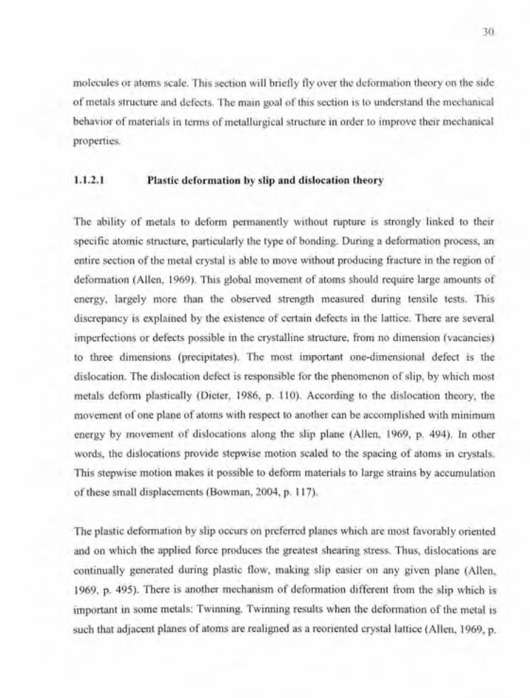
1.1.2.1 Plasti c déformation by slip and dislocation theory
The abilit y o f metal s t o defor m permanentl y withou t mptur e i s strongl y linke d t o thei r
spécifie atomi c stmcture , particularly the type of bonding. During a déformation process , an
entire section of the métal crysta l is able to move without producing fracture in the région of
déformation (Allen , 1969) . This global movement o f atoms should requir e larg e amounts of
energy, largel y mor e tha n th e observe d strengt h measure d durin g tensil e tests . Thi s
discrepancy i s explained b y the existence o f certain defect s i n the lattice . There ar e severa l
imperfections o r defects possibl e i n the crystalline stmcture , fro m n o dimension (vacancies )
to thre e dimension s (précipitâtes) . Th e mos t importan t one-dimensiona l defec t i s th e
dislocation. The dislocation defec t i s responsible for the phenomenon o f slip, by which most
metals defor m plasticall y (Dicter , 1986 , p . 110) . Accordin g t o th e dislocatio n theory , th e
movement o f one plane of atoms with respect to another can be accomplished with minimum
energy b y movemen t o f dislocation s alon g th e sli p plan e (Allen , 1969 , p . 494) . I n othe r
words, th e dislocation s provid e stepwis e motio n seale d to th e spacin g o f atom s i n crystals .
This stepwis e motion makes i t possible to deform material s to large strains by accumulatio n
of thèse small displacements (Bowman, 2004, p. 117).
The plastic déformation by slip occurs on preferred plane s which are most favorably oriente d
and o n which th e applie d forc e produce s th e greates t shearin g stress . Thus, dislocations ar e
continually generate d durin g plasti c flow, makin g sli p casie r o n an y give n plan e (Allen ,
1969, p . 495) . There i s anothe r mechanis m o f déformation différen t from th e sli p which i s
important i n some metals: Twirming. Twinning results when the déformation o f the métal i s
such that adjacent planes of atoms are realigned as a reoriented crysta l lattice (Allen, 1969 , p.

31
497). The mechanis m wil l no t be developed hèr e because i t i s not th e mechanism mvolve d i n
the studied materials .
1.1.2.2 Importanc e o f defect s
As discusse d earlier , th e plastic déformatio n o f crystal s i s directly linke d t o the movement o f
dislocations. Bowma n (2004 ) notifie s tha t nearly perfec t crystal s (wit h ver y few dislocations )
hâve a very hig h résistance to plastic déformation , bu t defor m a t relatively lo w stresse s afte r
dislocation multiplicatio n take n place . That i s to say , the capacit y to defor m a métal dépend s
on th e eas e o f dislocation s movement . So , i f th e dislocatio n encounter s a régio n wher e th e
atoms ar e displace d from thei r usua l positions , a highe r stres s i s require d t o forc e th e
dislocation t o pas s th e région . Discontinuitie s i n material s suc h a s vacancies , dislocations ,
grain boundaries , an d précipitâtes serve a s "stop signs " for dislocation s (Askelan d an d Phulé ,
2003, p . 159) . The strengt h o f a metallic materia l can , therefore , b e controlle d by controllin g
the numbe r an d typ e o f imperfections . Thus , strengthenin g mechanism s represen t th e ke y o f
the understanding fo r the déformation o f polycrystalline materials .
1.1.2.3 Strengthenin g mechanism s
There ar e three différent strengthenin g mechanisms based o n the three catégorie s of "defects "
in crystals . Th e poin t defect s suc h a s interstitia l atom s dismp t th e perfectio n o f th e crysta l
stmcture an d slo w dow n th e dislocatio n whic h ha s t o encounter . B y introducin g
substitutional o r interstitia l atom s a solid-solutio n strengthenin g i s caused . A s well , surfac e
imperfections suc h a s grai n boundarie s caus e th e sam e effect . A t eac h grai n boundary , th e
movement o f dislocation s i s blocke d an d highe r stresse s ar e neede d t o kee p slippin g th e
dislocation. Increasin g th e numbe r o f grain s lead s t o a n increas e o f grai n boundarie s so , a
grain-size strengthenin g take s plac e (Askelan d an d Phulé , 2003 , p . 160) . Finally , th e thir d
strengthening method , mos t commo n i n metalli c material s come s from dislocatio n defects .
The présenc e o f dislocation s alter s th e perfectio n o f th e crysta l an d thei r multiplicatio n
causes mor e sto p point s fo r th e dislocatio n motion . Thi s strengthenin g mechanis m durin g

32
defomiation b y increasin g th e numbe r o f dislocations i s called Strai n Hardenin g (Bowman ,
2004, p . 157) . Knowing tha t dislocatio n motio n cause s plasti c déformation , whe n ther e ar e
too man y dislocations , the y interfèr e wit h thei r ow n motion s i n additio n t o th e interactio n
with th e précipitâtes . Th e resui t i s a n increase d strength , henc e strai n hardenin g (Dicter ,
1986). Th e strai n hardenin g a s wel l a s th e amoun t o f précipitâte s influence s directl y th e
mechanical properties of the material.
1.1.3 Mechanica l point of view
Previously, materia l defomiatio n ha s bee n presente d wit h a metallurgica l poin t o f view . I t
has bee n show n tha t th e mechanica l propertie s o f metal s dépen d o n thei r metallurgica l
stmcture an d t o well-understan d thos e properties , i t i s necessar y t o understan d th e
relationship betwee n mechanica l behavio r an d microstructure . Now , th e mechanica l
properties ar e approache d a t the othe r en d o f th e scale : th e macroscopic level . A commo n
way to study the mechanical behavior of material is through standardized mechanical test s to
measure the properties.
1.1.3.1 Mechanica l properties définition s
The tension tes t is the most commo n method used to evaluate the résistance of a material t o
déformation an d failure . I t consist s o n stretchin g a uniform tes t spécime n alon g it s centra l
axis an d records simultaneousl y the increase of the uniaxial tensil e forc e an d the elongatio n
of the spécimen. Hère , a highlight i s made on th e response obtained afte r suc h a test. Mor e
détails abou t th e tes t i n practic e ar e availabl e o n sectio n 2.2.1 . Th e stress-strai n curv e i s a
représentation o f th e performanc e o f th e spécime n a s th e applie d loa d i s increase d
monotonically t o fracture (Moosbmgger , 2002) . Figur e I. I présent s a typica l stress-strai n
curve fo r a méta l obtaine d from th e load-elongatio n measurement s mad e o n th e tes t
spécimen.

33
/
E=S./s; (
i ' r
B là
/ ' l ;
1 !
1 ' II II r
Strair
Unifoirn strai n
'
""••"-YS (offset yi e d
strength}
iG fra cture
° - " - ^ ' ^ - ^ - * ' ' '
Necking begins
T e n stren
• - • u
~~'"- ~- L . 1
X 1 1
3i'e gih
Fracture
V A
f • • " 1
Fracture stress
0.202 Engîneeinng stra'n. e
Figure 1. 1 Typical engineering stress-strain curve. From Moosbmgger (2002)
The engineerin g stres s (S ) plotte d i n thi s diagra m correspond s t o th e averag e longitudina l
stress in the tensile spécimen obtained by dividing the applied load by the original area of the
cross sectio n o f th e spécimen . The engineerin g strai n (e ) i s th e averag e strai n obtaine d b y
dividing the elongation of the gauge length of the spécimen by its original length.
The engineering stress-strai n diagra m ca n be separated i n three parts. The linear segmen t o f
curve goes fro m th e origin, 0 to point A and i s called the elastic région. I n this portion , the
stress i s linearl y proportiona l t o th e strai n an d whe n th e stres s i s removed , th e strai n goe s
back to zéro. The most important elastic property is:
• The modulus ofelasticity or Young modulus (E): it corresponds to the slope of the elastic
part o f the stress-strain curve . I t is a measure of the stiffhess o f the material. The young
modulus i s relate d t o th e bindin g force s betwee n atoms . So , i t i s considere d
microstmcture insensitiv e sinc e it s value i s dominated b y th e strengt h o f atomi c bonds ,
which canno t b e modifie d b y microstmctur e features . O n th e othe r hand , i t ca n b e

34
affected b y crystal orientations . Heat treatments and cold work can modify E only if they
affect th e crystallographic orientations texture.
The second part of the stress-strain curv e corresponds to the uniform plasti c déformation .
In thi s région , fro m poin t A (o r B ) t o ultimat e tensil e strengt h (Su) , th e spécime n i s
permanently deformed eve n if the load is released to zéro. For most materials, the point at
which plasti c déformatio n begin s i s difficul t t o defin e wit h précisio n (Dicter , 1986 , p.
278). Various criteria for the beginning of yielding are used as shown in Figure 1.1:
• The proportional limit (A) is the leve l o f stres s abov e which th e relation betwee n stres s
and strain is no more linear
• The elastic limit (B) is the maximum stres s tha t ca n be applied t o the spécimen withou t
permanent déformation . I n othe r words , i t i s th e critica l stres s valu e neede d t o initiat e
plastic déformation . I n metals , thi s i s usuall y th e stres s require d fo r globa l dislocatio n
motion.
• The yield strength (YS) i s th e stres s require d t o produc e a smal l specifie d amoun t o f
plastic déformatio n usuall y define d a t a n offse t strai n valu e o f 0.2% . I t i s th e mos t
common paramete r use d t o defin e th e yiel d point . A s depicte d i n Figur e 1.1 , a lin e
starting wit h thi s offse t valu e o f strai n an d paralle l t o th e elasti c par t o f th e curv e i s
drawn. The stress value corresponding to the intersection o f this line and the engineering
stress-strain curv e is defined a s the offset yiel d point. The yield strengt h obtaine d by an
offset metho d i s widel y use d fo r desig n an d spécification s purposes , becaus e i t avoid s
subjective estimation of the plastic déformation starting point.
The strain hardening i s th e increas e i n th e déformatio n résistanc e o f th e materia l wit h
increasing strain . Th e volum e o f th e spécime n remains constan t durin g plasti c déformatio n
and a s th e spécime n elongates , i t cross-sectiona l are a decrease s uniforml y alon g th e gaug e
length. Durin g th e unifor m plasti c déformation , th e strai n hardenin g compensâte s fo r thi s
decrease in area and the engineering stress continues to rise with increasing strain . When the
stress reache s a maximum, th e decreas e i n spécime n cross-sectiona l are a become s greate r
than the increase in déformation load arising from strai n hardening and the neck occurs.

35
The lates t portio n o f th e stress-strai n diagra m goe s fro m S u t o fracture . I n thi s section ,
detonnation doe s not remain uniform . Som e properties ar e linked wit h thi s part :
• The Tensile Strength (Sj or Ultimate Tensile Strength (UTS) i s the stress obtained fo r th e
highest applie d force , whic h automaticall y correspon d t o th e maximu m stres s o n th e
engineering stress-strai n curv e fo r ductil e materials . Thi s valu e ha s onl y a littl e
ftindamental significanc e wit h regar d t o th e strengt h o f a materia l a s i t shoul d onl y b e
regarded a s th e measur e o f th e maximu m loa d tha t i t ca n withstan d unde r th e ver y
restrictive condition s o f uniaxia l loadin g (Dicter , 1986 , p. 278) . The neckin g effec t tend s
to distor t th e measurements sinc e i t i s difficul t t o compensat e fo r i t to calculat e th e actua l
local stres s strain values .
• The Necking strain (N %): A t som e point , a régio n deform s mor e tha n th e other s an d a
significant loca l decreas e i n th e cross-sectiona l are a occurs . Thi s phenomeno n i s know n
as neckin g an d wil l b e develope d i n sectio n 1.1.3.2 . Th e déformatio n reache d whe n
necking start s i s evaluate d a s th e neckin g strain , whic h correspond s t o th e strai n a t th e
tensile strength a s the elastic retum i s negligible in the studied materials .
• The Elongation (ef) or Breaking strain (A %) i s on e o f th e conventiona l measure s o f
ductility. Ductilit y measure s th e amoun t o f defomiatio n tha t a materia l ca n withstan d
without breaking . Th e elongatio n describe s th e permanen t plasti c déformatio n befor e
failure an d correspond s t o the engineering strai n a t fracture .
Others importan t concept s o n th e mechanica l behavio r o f material s hâv e t o b e define d i n
order to well-understand th e entire material déformatio n phenomenon :
• The true stress-true strain curve use s th e instantaneou s dimension s o f th e spécime n a t
each poin t durin g th e tes t fo r th e propertie s évaluatio n wher e a s th e engineerin g stress -
strain curv e use d th e initia l dimension s o f th e spécime n i n th e calculations . Beyon d th e
point o f maximum load , th e méta l continue s t o strai n harden s u p t o fracture. So , the tm e
stress increase s afte r neckin g because , althoug h th e loa d require d decreases , th e are a
decreases eve n more . Th e tm e stress - tm e strai n curv e i s ofte n calle d "flo w curve " whe n
considering onl y th e unifor m plasti c déformatio n zone . Th e équation s use d t o calculat e

36
the tm e stres s strai n value s ar e base d o n th e volum e constanc y assumptio n an d ar e
expressed i n the foUowing terms :
<7ti-ue = (7eng( l + ^eng ) ( 1 - 1 )
£tme = l n ( l + S e n g ) ( 1 . 2 )
1.1.3.2 Th e neckin g phenomeno n
Necking ca n b e define d a s a non-unifor m o r localize d plasti c déformatio n resultin g i n a
localized réductio n o f cross-sectiona l are a o f a tensil e spécimen . Thi s phenomeno n i s see n
only in a tensile tes t an d corresponds , i n most cases , to a mechanical instabilit y in tension an d
not a damage problem. The necking begins a t maximum loa d where the increase i n stress du e
to decreas e i n th e cross-sectiona l are a o f th e spécime n become s greate r tha n th e increas e o f
stress du e t o strai n hardening . Th e formatio n o f a neck i n th e tensil e spécime n introduce s a
complex triaxia l state of stress in that région .
1.1.3.3 Materia l work hardenin g descriptio n
In orde r t o easil y describ e th e stress-strai n curve s an d strai n hardenin g behavio r o f metalli c
materials, flow curve s o f metal s ar e usuall y describe d b y mathematica l expressions . I n th e
case o f col d working , th e hardenin g o r constitutiv e équatio n i s expresse d a s foUow s ap =
f{£p). Th e mos t commo n expressio n describin g th e strai n hardenin g behavio r i s a simpl e
power la w relation between tm e stress an d tme plastic strain :
a = Kxsp" (1.3 )
Where n i s the strain hardening exponen t an d K th e strength coefficient .
Based o n th e powe r la w équatio n an d afte r severa l calculations . Dicte r (1986 , pp . 289-292 )
suggests a simple relationship fo r th e strain a t which neckin g occurs :
£u = n (1.4 )
Where £„ is the tme uniform strai n and n is the strain hardening exponent .

37
• The strain hardening coefficient (n) i s define d a s a paramete r tha t describe d th e
susceptibility o f a material t o work harden . I t évaluâtes the effec t tha t strai n ha s o n th e
resulting strengt h o f th e material . Thi s dimensionles s coefficien t i s calculate d b y th e • d{lna) , • „ , , ratio — (Kleemol a and Nieminen , 1974).Th e parameter n is schematically the slope
a{lnE)
of the plastic portion of the tme stress-tme strain curve when plot on a logarithmic scale.
The strain hardening exponen t value s vary between 0 and 1 , from perfectl y plasti c solid
to an elastic solid.
• The strength coefficient K i s a n expérimenta l constan t compute d from th e fit o f dat a t o
assume power curve according to the American Societ y for Testing and Materials (2000).
It i s equa l t o th e tm e stres s a t Sp=l.Th e strengt h coefficien t doe s no t hâv e a physi c
meaning, it is just a fitting parameter with units of stress.
Déviations from E q 1. 3 ar e frequentl y observed , particularl y a t lo w an d hig h strains . A s a
resuit, severa l empirica l équation s hâve been proposed t o describe expérimenta l stress-strai n
curves. Hère, five of the most common relations hâve been treated and are presented below:

38
YS* K
YS / '
0 a ) Hollomon 1 ^ b ) Ludwik 1
« i
YS À
i
.....-.^,„.,.,.......,.^...„.^^
^ : ï ï
a
UTS
YS
-eOO c ) Swift 1 • - B
K + exp(Kl-nl)
exp(Kl)f
'•' "-'//i-M»'*^^^'^;
0 d ) Voce 1 ' • e
0 . . . 1 e) Ludwigso n
..„ e
Figure 1.2 Schematic représentation of the usual hardening équations. adapted from Montheille t (2008)
• The Hollomon équation (Figure 1.2-a):
a = KH^ep" (1.5 )
The Hollomon équatio n is équivalent to the power équation given above . The yield strengt h
associated to this relation is nuU because it corresponds to sp=0. This very simple équation is
suitable for low to médium carbon steels and low YS alloys (Montheillet, 2008).
• The Ludwik équation (Figure 1.2-b):
a = G o + KLKX£p " (1.6 )
The Ludwi k équatio n allow s t o introduc e a YS criterion (ao ) an d KL K an d n, équivalen t
parameters i n analogy to the Hollomon relation . Actually , the Ludwik curv e is obtained by
translating the Hollomon curve parallel to the stress axis and shift to YS quantity.

39
• The Swift équation (Figur e 1.2-c) :
a = K s X (80+Sp)" (1.7 )
The swif t équatio n propose s anothe r strateg y t o introduc e a no n nul l stres s fo r zér o plasti c
strain. Th e curv e i s obtaine d b y a translation o f th e Hollomo n la w paralle l t o th e strai n axi s
and shif t t o -so quantit y (Montheillet , 2008) . Swif t an d Ludwi k équation s ar e generall y use d
when th e user do not want t o ignore the YS.
• The Voce équation (Figur e 1.2-d) :
a = av - K v X exp (nySp) (1.8 )
Hère, K v an d n y ar e materia l constant s tha t diffe r fro m th e usua l K an d n presente d u p t o
now. (J v represents th e constan t reache d whe n th e strai n goe s t o infinity , i n othe r word s th e
UTS. Thi s équatio n refer s t o th e dynami c recover y mechanism s a t larg e déformation s an d i s
generally used fo r larg e strains and fo r hot working applications .
• The Ludwigson équation (Figur e 1.2-e) :
a = KLX Sp"+exp(Ki+ni£p) (1.9 )
This équatio n i s suitabl e fo r material s whic h deviat e markedl y from équatio n (1.3 ) a t lo w
strains (Dicter , 1986 , p . 288 ) suc h a s austeniti c stainles s steels . Ex p (Ki ) i s approximatel y
equal t o the proportional limi t (Figur e 1. 1 poin t A ) an d n i allow s the déviation o f stress fro m
équation (1.1 ) to be quantified .
Ail th e presente d mathematica l équation s aime d t o describ e th e hardenin g behavio r o f
materials but the y are completely empirica l an d do not contai n an y mechanisms behind them .
1.2 Characterizatio n différence s betwee n tubes an d sheet s
The objectiv e o f th e wor k i s t o characteriz e variou s material s fo r tub e hydroformin g
applications. U p t o now , peopl e use d t o wor k wit h materia l propertie s o f th e flat shee t from
which th e tub e i s made . Th e propertie s ar e measure d fro m tensil e testin g o f th e shee t méta l

40
prior t o roUin g (Sokolowsk i an d al. , 2000) . Bu t th e tub e makin g proces s ma y hâv e a n
influence o n th e mechanical an d microstmctura l properties . I n fact , roUing , welding, sizin g
subséquent opérations consume part o f the formability o f the sheet métal. Thus any material
properties suc h a s flow stress, strain hardening , yiel d strength , etc . may not be the sam e fo r
sheet an d tube eve n i f they com e fro m th e same grade and compositio n shee t (Koç , Aue-u-
lanand Altan , 2001).
Actually, ther e are several methods t o manufacture tube s and depending o n the one chosen ,
the impact on the formability differs :
1. Th e most common, cheapest but wors t method o f producing large quantities of tubes fo r
HF applications is roll-forming foUowed by a welding process. The weld seam in the tube
leads t o a non-homogeneity i n th e materia l propertie s an d i s on e o f th e leas t deforme d
régions of a hydroformed part . Some studies hâve been done on quantifying th e available
formability used up during tube making and hâve been summarized by Koç (2008, p. 96).
He concludes that the method proposed eve n if it provides an approximate assessment of
the amoun t o f formabilit y use d t o for m a flat shee t int o a tube , thi s effec t strongl y
dépends on the tube making method and may vary from on e set-up to the other.
2. Tubes , as in our case, can be made by extmsion. This method is interesting because there
is no weld line but one of its main drawbacks is the non uniformity o f the wall-thickness
around the cross section (Koç , 2008, pp. 95-96). In addition, the extmsion process being
spécifie, i t générâtes errors to use the material properties comin g from a laminated shee t
to attempt characterize an extmded tube.
Another issue with the material characterization metho d for tubes is the testing methods. The
simplest wa y to obtain formabilit y measurement s i s to conduct a tensile test. Tensile testing
on spécimen s eu t from tube s ca n b e on e wa y t o obtai n materia l propertie s o f th e tubes .
However, th e accuracy an d appropriatenes s o f thèse results fo r hydroformin g purpose s ma y
be questionable. Koç and al. (2001) gives thèse three reasons:
In orde r t o tes t th e spécimen s eu t fro m tubes , curvatur e du e t o tubula r for m ha s t o b e
straightened. This would alter the specimen's properties.

41
Tensile testin g i s don e unde r uniaxia l loading , an d henc e uniaxia l stat e o f stres s exist s
whereas in HF biaxial even triaxial state of stress also exists.
The friction conditio n m HF process may not be repeated in tensile testing method.
The différenc e o f th e stat e o f stres s i n tensil e tes t compare d t o th e on e undergoin g durin g
hydroforming lead s t o a n under-estimatio n o f th e strai n localizatio n durin g HF . I n othe r
words, the necking seems to occur prematurely in a tensile test than in a HF. The true stress-
tme strain curve has to be extrapolated in order to try reach the level of déformation expecte d
in HF and a new criterion has to be found .
To b e abl e t o carefull y characteriz e th e aerospac e alloy s fo r H F applications , variou s
characterization methods hâve been tested, from uniaxia l test of flat sheets to biaxial test s on
tubes.
1.3 Aerospac e alloys
In orde r t o stud y th e propertie s o f shee t metal s fo r aerospac e applications , investigation s
were performed o n various material s tha t ar e représentative o f PWC production . Austeniti c
stainless steel s ar e used fo r application s requirin g high mechanica l propertie s an d moderat o
corrosion résistance , while martensitic stainles s steel s ar e used fo r component s designe d fo r
higher températures applications and superalloys as well.
1.3.1 Stainles s Steel 321
Stainless Stee l (SS ) 321 is not a conventional aeronautica l alloy , even i f it can be foun d fo r
particular aerospac e application s (Mokrzyck i an d Savoie , 2006) . Thi s allo y i s a perfec t
candidate for this work as it is relatively easy and cheap to get and can be used to put in place
the characterization methods . Therefore, a complète study has bee n conducte d o n thi s allo y
for both, tubes and sheets.

42
1.3.1.1 Chemical compositio n
SS 32 1 i s a n austeniti c chromiu m - nicke l stainles s stee l stabilize d b y titaniu m agains t
intergranular chromiu m carbid e précipitation . I n thi s typ e o f steel , carbo n combine s
preferentially wit h titaniu m t o for m harmles s titaniu m carbide s an d leave s chromiu m i n
solution t o maintai n ful l corrosio n résistanc e (Boyer , 1990 , p . 203) . Tabl e 1. 1 give s th e
chemical composition of the SS 321.
Table 1. 1 Chemica l composition of SS 321 From Chandler (1996)
Elément
Carbon
Manganèse
Phosphorus
Sulfur
Silicon
Chromium
Nickel
Titanium
Nitrogen
Iron
%weight
0.08
2.0
0.045
0.03
1.0
17.00-19.00
9.0 - 12.0 0
>5 X %C, < 0.70
<0.I0
balance
1.3.1.2 Mechanical properties
S S 32 1 i s extremel y toug h an d ductile , an d respond s wel l t o dee p drawing , bendin g an d
forming. I t can be harden onl y by cold work . Annealin g hea t treatment s ar e used t o relieve
stresses, increase softnes s an d ductility , a s well a s to provide additiona l stabilizatio n agains t
Chromium carbid e formatio n (Chandler , 1996) . Représentative tensil e propertie s o f S S 32 1
in th e anneale d conditio n a s wel l a s stress-strai n curve s fo r différen t déformatio n

43
températures can be foun d i n the literature (Boyer , 1990) . Table 1. 2 provide s the tension o f
annealed SS 321 at room température. On Figure 1.3 , the stress-strain curves under tension at
various température levels are plotted.
Table 1. 2 Typical tensile properties of stainless steel 321 From Boyer (1990)
SS321 Condition
annealed
0.2% Yield strength (MPa)
240
Tensile strength (MPa)
620
Elongation (%)
45
Elastic modulus
(GPa) 193
Hardness (HRB)
80
80
6-0
^^ 1Â
40
20
T^ :
" o 0,0 8 0.1 6 3trisir<
• 120 0
80 " F <27 ' O
- 40 0 ' F (20 4
aOO "F (42 7 'C
"F (64 9 " O
"O
:>
0,24 0,3 2 , iii./in .
660
420 m O. -a:
2S0
140
0.40
Figure 1.3 Stress- strain curves of SS 321. From Boyer (1990)
1.3.2 Stainless Steel 17-4 PH
Stainless stee l 17- 4 PH i s a very interesting allo y fo r aerospac e application s becaus e o f it s
high toughnes s an d despit e it s limited déformatio n possibilities . Moreover , it s sensitivit y t o
heat treatments makes i t attractive fo r hydroforming. Fo r instance, in the case of multi-stage

44
forming processes , intennediat e hea t treatment s restor e th e fonnabilit y use d u p b y previou s
opérations an d enabl e to envisag e larg e cumulative strainin g an d comple x defomiatio n paths .
Because o f materia l availabilities , th e focu s o f th e wor k wil l b e onl y o n shee t material . Th e
challenge wit h thi s allo y i s t o characteriz e i t i n severa l hea t treate d condition s an d find th e
best metho d t o exten d it s formabilit y t o mak e i t hydroformable . Th e hea t treatment s
experimented wil l be limited to those already in use a t PWC.
1.3.2.1 Chemical compositio n
Table 1. 3 give s the chemica l compositio n o f SS 17- 4 PH.
Table 1. 3 Chemica l compositio n o f SS 17- 4 PH From ASM Internationa l (2002 )
Elément
Carbon
Manganèse
Phosphorous
Sulfur
Silicon
Chromium
Nickel
Copper
Niobium & Tantalu m
Iron
% w t
<= 0.0 7
<= 1.0 0
<= 0.0 4
<= 0.0 3
<= 1.0 0
15.00-17.50
3.00-5.00
3 .00-5.00
0.15-0.45
balance
As show n i n Tabl e 1.3 , th e importan t quantit y o f chromiu m give s t o thi s allo y a hig h
corrosion résistance . I n addition , th e présenc e o f coppe r wil l pla y a n importan t rôl e i n th e
metallurgical behavio r o f thi s alloy . Du e t o it s composition , S S 17- 4 P H i s a précipitatio n
hardening martensiti c stainles s steel . I t ha s th e uniqu e abilit y t o develo p hig h mechanica l

45
strength with relatively simple heat treatments and without any loss of ductility and corrosion
résistance. Thi s i s mad e possibl e b y th e us e o f on e o r both o f th e hardenin g mechanisms :
martensitic fomiation an d précipitation hardening (Peckner and Bemstein, 1977 )
1.3.2.2 Mechanica l properties and microstructure
Alloy 17- 4 P H has a martensitic stmctur e an d possesses th e highes t possibl e yiel d strengt h
among the précipitation hardening stainless steels . This alloy is most often supplie d fro m th e
mill in solution-annealed state (condition A). Its microstmcture i s composed o f a low-carbon
martensite and up to several volume percent of ô-ferrite stringers (Wu, 2003). By subséquent
précipitation hardenin g treatment s o n th e solutio n anneale d condition , a wid e rang e o f
mechanical propertie s ca n be obtained. Severa l studie s o n précipitation mechanis m o f 17- 4
PH stainless stee l are based on the fact tha t its précipitation seems to be essentially the same
as i n Fe-C u an d Fe-Cu- X allo y (Russe l an d Brown , 1972 ; Youl e an d Ralph , 1972) .
Précipitation start s wit h th e formatio n o f cohéren t coppe r rich clusters , which, afte r furthe r
aging, transfor m int o incohéren t FC C s-coppe r précipitâtes . 17- 4 P H ca n b e variousl y
hardened t o obtai n th e desire d properties . Mos t commo n hea t treatment s lea d t o unage d
(condition A) , peak-age d (H900 ) an d over-age d (H1150 ) conditions . Tabl e 1. 4 give s th e
mechanical properties of 17-4 PH for thèse différent conditions .

46
Table 1.4 Typical mechanical properties of 17-4 PH From Peckner and Bemstein (1977)
Form
Sheet cold
flattened
Condition
Condition A H 9 0 0 / r
H1150/4"
0.2% yield strength (MPa)
1000 1379 1034
Tensile strength (MPa)
1103 1448 1103
Breaking Elongation
(%)
5.0 7.0 11.0
Elastic modulus
(GPa)
-199.9 200.6
Hardness (HRC)
35 45 35
Figure 1. 4 provide s stress-strai n curve s of a SS 17- 4 PH bar from room températur e (24°C)
to elevate d température s (48 2 °C) . Figure 1. 5 als o présent s the stress-strai n curve s o f 17- 4
PH alloy in the various heat treated conditions specified i n Table 1.4.
175
150
125
100
75
50
25
75 •F (? 4 - C )
- ' TOO "
"•" 9 0 0 -
F (20 4 °C )
'- (37 1 ' O
= (48 2 " O
1050
700
4 6 8 Strain, 0,00 1 in,,1n .
Figure 1.4 Stress-strain curves of 17-4 PH bar at various températures.
From Boyer (1990)
* Hardening at 900T ± 15° F (482°C ± 9°C) (iuring Ih . " Hardenin g at 1150 T ± 15 T (621°C ± 9°C) during 4 h.

47
Q_
35
1200
1000
800
600
400
200
-
/
7 / 1
y^-*^'*-'"^
1
—
-mi r
----
'¥
" "—*v„^
C" H 1 1 50
1
-f H90 D
Condi t ion A ' ' M J , ,
17-4 P H Stroke Rat e - 0 5 mm,'n-i n 300 " C
1 1 1 0.00 0.06 0 0 9
Strain (mm/mm )
Figure 1.5 Stress-strain curves of 17-4 PH at différent conditions.
From Wu (2003)
The main observation extracted from thèse results is that in this alloy the necking occurs very
early (aroun d 4% ) and an importan t déformatio n afte r neckin g i s observed . Th e strai n
reached befor e nec k seem s t o be the highest i n condition A but significant serration s are
observed on the condition A curve. Thèse serrations wer e interprete d by Wu (2003) durin g
his thesis as dynamic strain aging in 17-4 PH.
1.3.3 Superalloy Inconel 718
Inconel 71 8 (nSfC7I8) i s the only superallo y studie d i n thi s work . I t is one of the most
widely-used nicke l superalloy s an d ha s excellen t physica l propertie s whic h mak e i t
interesting for extensive use in aerospace components.
1.3.3.1 Chemical composition
INC718 exhibits excellent physical an d mechanical properties , which remain from cryogénie
to elevate d température s (0.8xT°f) . I t maintain s hig h strengt h an d excellen t corrosio n

48
résistance at high températures (Song and Huh, 2007). The chemical composition o f INC718
is presented in Table 1.5 .
Table 1. 5 Chemical composition of INC 718 From Boyer (1990)
Elément
Carbon
Silicon
Manganèse
Copper
Nickel
Chromium
Niobium & Tantalu m
Molybdenum
Aluminum
Titanium
%wt
<=0.10
<= 0.7 5
<= 0.5 0
<= 0.7 5
50.00-55.00
17.00-21.00
4 .50-5 .75
2 .80-3 .30
0 .20-1 .00
0 .30-1 .30
1.3.3.2 Mechanical properties and microstructure
INC 718 superalloy consists of an FCC y-matrix with intergranular (3-precipitates , (Nb, Ti) C
carbides an d a hig h volum e fractio n o f embedde d y ' an d y " précipitâte s (Son g an d Huh ,
2007). Thès e précipitâte s impar t reasonabl y hig h tensil e an d cree p strengt h a t elevate d
températures while maintaining adéquate ductility, fractur e toughnes s an d fatigue properties .
According t o th e literatur e (Slam a an d Cizeron , 1997) , th e variou s hardening carbide s ar e
formed jointly or successively depending on the température range and the aging time.
The tensil e propertie s o f rNC71 8 allo y a t roo m températur e chang e accordin g t o différen t
heat treatment conditions , as presented in Table 1.6 .

49
Table 1.6 Typical mechanical properties of INC 718 From Boyer (1990)
Conditions
Cast& *
Age-Hardened Annealed Annealed &
Age-Hardened
0.2% yield strength (MPa)
828
414
1034
Tensile strength (MPa)
1000
897
1310
Breaking Elongation (% )
10
45
25
Elastic modulus
(GPa)
-
204
-
The stress-strain curv e of INC718 armealed and aged bar a t room an d elevated température s
is presented in Figure 1.6 and his tensile properties as a function o f température in Figure 1.7.
240
200
160
120
14 )C ' F {7 f 0 -C )
70 " F ( :
12(
.1 -C )
JO ' F (64 9 'C )
1680
840
560
0 2 4 6 8 Strain. %
10 1 2 1 4 1 6
Figure 1.6 Stress-strain curve of Inconel 718 bar at various températures.
From Boyer (1990)
' Age-Hardenin g a t 1325"? (718°C) during 16h
" Annealin g at 1750T (955°C) during I h

50
200 (1379)
160 (1103)
Q.
— 12 0 j£ (327 ) </> (fi
" 8 0 (552)
40 (275)
0
93
.
0 20 0
Température, ° C
20^ 31 6 42 7 53 a 64 9 { 1 1 1 1
Tensile strength — - ^
Yield strength ~ ' " " ' \
Elorîgation
1 1 1
400 60 0 80 0 100 0 120 0 Température, ° F
760
1400
871 1
1600
982
) 1800
1093
\
-
2000
200
160
120 1 m en c: o
UJ 80
40
0
Figure 1.7 Tensile properties of aged Inconel 718 bar. From Spécial Metals Corporation (2007)
As can be seen from thèse figures, INC718 has a wide plastic range which is interesting fo r
déformation by hydroforming.
INC7I8 is the most concemed material in the global project. It s complex microstructure with
several précipitâtes is interesting to study, notably thanks to the effects o f heat treatmen t on
its micro structures and hardening potential. However, it is very expensive and difficult t o get.
So, very little work has been conducted on this material available only in sheet form.

CHAPTER2
EXPERIMENTAL PROCES S
The expérimenta l test s wil l allo w documenting th e mechanical behavio r o f each material. I t
is therefore ver y importan t t o track precisel y sampl e déformations durin g th e tests. For tha t
reason, tw o différen t method s fo r déformatio n measuremen t hâv e bee n tested . A video -
extensometer, availabl e a t ETS, was used to measure déformation by tracking the movement
of some dots marked on the spécimen and an Aramis system, an optical grainy pattem image
corrélation throug h a 3 D déformatio n measurement , whic h wa s se t u p a t AMTC . Also ,
différent mechanica l testin g methods use d i n the présent work ar e presented i n this section ,
namely: uniaxial tensile testing and free expansion testing also called hydro bulge testing.
2.1 Déformatio n measurements methods
Tensile tests hâve been chosen to compare both déformation trackin g methods as it is one of
the most commonly used tests for evaluating mechanical behavior of materials under uniaxial
loading. I t consist s o f slowly pulling a sample of materia l i n tension unti l i t breaks . Durin g
the test , force-displacemen t dat a ar e monitore d an d recorde d t o provid e a quantitativ e
measure o f ho w th e tes t ite m defomi s unde r a n applie d tensil e force . Bot h video -
extensometer an d Arami s syste m giv e informatio n o n th e specimen' s extensio n b y using a
slight différent way .
The video-extensomete r measure s th e displacemen t betwee n dot s wherea s Arami s record s
the déformation o f th e points painte d o n the sample . The video-extensomete r canno t repor t
accurately th e occurrenc e level , intensit y an d origi n o f strai n localization . Th e déformatio n
dépends o n th e positio n o f th e failure . Thi s inaccurac y ma y generat e error s an d infer s
imprécision around the video-extensometer method. The Aramis method covers a larger zone
of déformatio n whic h wil l includ e inevitabl y th e failure . However , th e frequency o f th e
images recor d i n th e cas e o f Arami s i s limite d b y th e capacit y o f th e compute r use d an d
becomes fa r les s tha n i n th e video-extensometer . Thi s ma y b e a drawbac k o f th e Arami s

52
method. Th e classica l extensometer s hâv e no t bee n teste d becaus e o f thei r mai n drawbac k
which i s th e possibl e damag e o f th e sampl e du e t o th e contact . T o se t u p th e bes t
characterization metho d i n ou r case , i t i s importan t t o compar e bot h déformatio n
measurement method s i n orde r t o choos e th e appropriat e one . Th e latte r wil l b e use d t o
extract th e strain s whic h wil l allo w th e évaluatio n o f th e hardenin g coefficient s i n fiirther
constitutive équations.
To illustrat e th e différen t déformatio n measuremen t methods , dat a plotte d i n thi s sectio n
comes from results obtained on 17- 4 PH spécimens extracted from sheets in the as received
state (Conditio n A ) a s specifie d i n AST M Spe c A 8 (ANNE X I) . The teste d sample s wer e
taken along the rolling direction (RD) of the sheet. Figure 2.1 shows the relative direction of
the samples to the processing geometry.
SîieelorSîrip ,^~. QumWfWMh
/ \ Locatio n
WT^ CoM Safflpf e
D " T 0
^ v .
Dîip
t
" t = 3 \ X \ ^•r
icale Spesiraens
41 m i T
L = Longitudinal
D = Diagonal (45^)
T = Transverse
Figure 2.1 Location of sampling for tension testing of sheet products
2.1.1 Video-extensometer metho d
A vide o extensomete r i s use d fo r no n contac t an d accurat e déformatio n measurement s
without th e drawback s o f contac t extensometers . Furthermore , i t allow s t o documen t usua l
tensile properties (yield strength, ultimate tensile strength and elongation).
" Selected stamping and formability measurements : http://www.a-sp.org/database/viewsec.asp?sec=59 4

53
2.1.1.1 Procédure
The video-extensomete r use d i s a Messphysi k ME-46 . Th e syste m comprise s a vide o camér a
DCC, severa l lenses , a compute r wit h th e applicatio n software . Prio r t o test , th e width s an d
thicknesses o f the spécimens are measured a t three différen t location s alon g the gauge lengt h (a t
both end s an d a t th e middl e o f th e gaug e length ) usin g a caliper . Then , nin e dot s ar e draw n
manually wit h a permanent marke r a t the middle o f the gauge lengt h wit h a spécifie pattem a s
presented r n Figure 2.2 . During the tensile test, the position i n 2D of each dot i s recorded wit h
a hig h spee d camér a (registere d marks) . Wit h th e ai d o f measuremen t softwar e (Do t
Measurement), the points are numbered, digitized and so that the distance between points 1 and 3
is always equal to one. In order to get valid results, contrast between the dots and the background
is maximized. Fo r that reason, light intensity has to be adjusted usin g a lens diaphragm.
/ ^
l»1 • .
u Figure 2.2 Positio n an d numberin g
of measurement dots .
The test s wer e conducte d o n a MI S machin e (série s 810 ) wit h hydrauli c fixtures , availabl e a t
ETS. Amplificatio n module s wer e use d fo r a maximu m loa d o f lOOk N an d a maximu m
displacement o f 10 0 m m (Figur e 2.3) . Th e positio n o f dot s an d th e forc e / displacemen t
parameters o f the tensile machine are recorded a t 33 Hz whereas the position of points along both
axis ar e recorde d i n the directio n o f the applie d loa d ( X axis ) an d i n the transvers e directio n ( Y

54
axis) i n a tex t file a t th e rat e o f 4 Hz . The loadin g rat e i s 0.06 m m pe r second . Thès e number s
hâve been chose n t o remain consisten t compar e t o previous wor k done by PWC (Mokrzyck i an d
Savoie, 2006) . The différenc e betwee n th e recording frequencie s ma y affec t th e précision o f th e
test but the relatively slo w testin g rat e compensâtes for th e loss of data. The load i s recorded an d
will be used to calculate the stress . The position o f dots will be used for strai n calculations. Thèse
data will allow the évaluation of stress-strain curves .
MTS machine
Light
Video-extensometer
Tripod
Figure 2.3 Tensile test with video-extensometer assembly .
2.1.1.2 Preliminary result s on 17- 4 PH
The test s hâv e bee n conducte d o n si x 17- 4 P H sample s i n rollin g directio n (RD ) randoml y
chosen. The stress-strai n curve s obtained ar e presented i n Figure 2.4 .

55
1400
1200
m 2 1000
01
tu) _C 'C Ci 01
c
800
ÔOO
~ 4'"» 0
c UJ
200
0.02 0.0 4 0.0 6 0.0 8 0. 1 0.1 2 0.1 4
Engineering strai n
Figure 2.4 Tensile engineering stress-strain curves for 17-4 PH RD direction.
The behavior of the tested samples is reproducible from th e elastic part up to the YS. But, a
big différence betwee n th e firs t five samples (RD- I t o RD-5) an d the sixth on e is observed .
The stress-strai n curve s ar e quit e différen t afte r th e nec k poin t an d th e mptur e strai n goe s
from 5 % t o almos t 1 2 % fo r th e sam e material , th e sam e direction . Th e onl y différenc e
between thos e sample s i s th e positio n o f th e neckin g relativ e t o dot s locatio n a s show n i n
Figure 2.5.

56
Figure 2.5 17-4 PH RD broken samples: 1) Failure outside the dots (RD-1) 2) Failure inside the dots (RD-6).
If the necking appears between the 9 dots, the distance between the upper dots and the lower
ones increases dramaticall y an d the recording strain s take into account th e necking strai n in
addition t o th e conventiona l plasti c déformation . Thi s issu e cause s a significan t an d no n
negligible erro r i n th e évaluatio n o f th e neckin g strain . Fo r instance , th e neckin g strai n
obtained in the case of sample RD-6 is about 6.5% when in sample RD-1 we hardly reach to
3%. I n fact , i f mpture takes place outside the dots, the recorded déformation coul d be lower
than the actual déformation sinc e it can be far from th e recorded part of the sample. This can
suggest tha t a failur e eithe r insid e o r outsid e th e dot s doe s no t reflec t th e rea l plasti c
déformation.
2.1.1.3 Advantages / Drawbacks of video-extensometry
The video-extensomete r i s a widel y use d metho d t o measur e déformation . It s principa l
advantage is the easy set up. It takes generally les s than an hour to prépare a test. I t is also a
very accurate method for calculating some mechanical properties such as the elastic modulu s
and th e yiel d strength . However , thi s metho d présent s on e importan t drawbac k concemin g
the évaluation of the necking strain . The stress-strai n curv e shape obtained a t the end of the
test widely dépends on the position of the failure (insid e or outside the dots). This aspect will

57
bring important error s on the évaluation of the hardening laws since a maximum précisio n is
required on the déformation measurement .
To counte r pass thèse issues, the Aramis® system , which ca n be considered a s an improved
video-extensometer wit h tw o caméra s instead o f onl y one , has bee n teste d o n th e 17- 4 PH
spécimens.
2.1.2 Strai n fîeld measurement method by image corrélation of random pattern
The Aramis system is a non-contact optical 3D déformation measuring system. It documents,
analyzes, and calculâte s the distribution o f material déformation . Th e graphica l présentatio n
of the measured variable s pro vides a convenient understandin g o f the sample' s behavior . I t
can be used fo r tensil e testing or more comple x formin g processes , suc h a s free expansion .
The Arami s syste m ha s quit e a wid e rang e o f applications . I t ca n recor d dat a wit h loca l
resolution, high 3D strain field accuracy under static and dynamic loading.
2.1.2.1 Descriptio n of the method
The Aramis system consists of a sensor with two CCD caméras (for 3 D set up), a trigger box
to synchroniz e image s wit h othe r proces s parameter s a t a hig h fram e rate s an d a hig h
performance P C syste m wit h Arami s applicatio n software . Figur e 2. 6 show s th e différen t
parts of the Aramis system.

58
Right light
2 caméras
Tripod
Figure 2.6 Aramis system components.
The Arami s softwar e permit s th e specimen' s surfac e geometr y t o b e recognize d b y digita l
images and allocates coordinates to the image pixels. The first coordinates are gathered when
recording th e référenc e condition . Thi s imag e i s th e undeforme d stat e o f th e spécimen .
During sample déformation, further image s are recorded. Aramis observes the déformation of
the spécimen through th e images by means of a large number of square image détails called
facets. A face t i s a smal l squar e o f 1 5 x 1 5 pixels whic h i s approximatel y th e siz e o f on e
black dot. Each image is divided into many facets. The facets ar e identified b y the individual
gray level stmcture s o f the individual pixel s within the facet. Th e system détermines the 2D
coordinates o f th e facet s fro m th e corne r point s an d th e resultin g centers . Usin g

59
photogrammetric methods , th e 2 D coordinate s o f a facet , observe d b y th e lef t an d right
caméras, lea d t o th e calculatio n o f the 3' ' ' dimensional coordinate . A color spra y pattem o n
the spécime n surfac e i s necessary , especiall y fo r homogeneou s surfaces ' spécimens . I f th e
speckle patte m i s sufficientl y stochastic , eac h face t présent s a unique patte m o f a few dot s
within the image so that the software ca n calculate the position as well a s the déformation o f
the facets alon g the test through the recorded images. The spécimen déformation i s calculated
by comparing the dots position an d shape on the déformation stage s to their position o n the
first imag e correspondin g t o n o déformation . Arami s syste m i s use d t o measur e wit h hig h
temporal and local resolution a s well as high accuracy, 3D déformation and strain in material
spécimens.
2.1.2.2 Procédur e
The Aramis se t up procédure is divided in four steps : painting, calibration, the test itself and
the computation.
Painting
The Aramis ability to capture strains during the déformation i s closely bounded to the quality
of the paint applied to the samples. The biggest issue is to obtain maximum contrast between
the white paint an d the black dot s randomly spraye d o n ail samples . The white paint shoul d
be flat to avoid reflection an d thin enoug h to avoid unsticking . A distance o f approximatel y
15 cm shoul d be considered betwee n th e sprayer an d the sampl e i n order t o ge t th e desired
layer of paint. To apply the black dots, an airbmsh i s used instead of a black spray . To obtain
a goo d contrast , th e operativ e pressur e o f th e airbms h shoul d b e aroun d 20 0 Kp a (3 0 Psi )
with a distanc e o f abou t 2 meter s fro m th e sample . Otherwis e th e dot s migh t b e to o big .
Figure 2.7 shows an example of a good painting pattem.

60
Figure 2.7 Example of a good pattern.
Calibration
The secon d concern i s the calibration o f the Aramis system. This step allows calibrating the
software wit h the proper distance s between th e caméras and the sample a s well a s adjustin g
the caméras ' angle . I n other words , the calibration ste p allows the syste m t o be a t a known
distance fro m th e sampl e an d i t shoul d observ e clearl y the whol e spécime n durin g th e ful l
test. Th e lightin g i s als o a n importan t paramete r t o take int o accoun t fo r prope r results . I n
fact, th e entir e spécime n ha s t o b e uniforml y enlightene d wit h n o par t i n th e darknes s t o
avoid some missing data . This part is very critical and should be conducted ver y carefully t o
get the best out o f the system. Also, whenever the calibration i s done, nor the tripod nor the
caméras should be moved during the test, otherwise the calibration has to be redone.
Test procédure
After th e calibration , th e tes t can be carried out . The Aramis procédure for both tensil e an d
free expansio n tests is quite similar and only the procédure of the tensile test is detailed hère .
The sample is fixed onto the tensile machine. The test is started manually at the same time on
both: the tensile machine and the Aramis system. Aramis captured images at the frame rate of
3 Hz . A t th e en d o f th e test , ai l the stage s (correspondin g t o each image ) i s compute d an d
post processed in order to extract the desired data; for example the strains values. The images
could be assembled to record a movie or just to see the strain localization (necking) . The load
levels ar e obtained b y extracting data from th e tensile machine an d i n order to calculate th e
local stress field .

3D Computation
At th e en d o f th e test , a computatio n i s neede d t o extrac t th e déformation . Fo r face t
computation, th e définitio n o f the startin g poin t i s required . Th e startin g poin t i s manuall y
chosen o n th e first imag e (n o déformation ) b y th e operator . I n bot h camér a image s thès e
points are marked. The computation par t consists on putting together the images captured by
each camér a t o reac h a 3 D leve l an d calculat e th e strain s base d o n th e displacement s an d
shapes of the facets inside the images.
2.1.2.3 Preliminar y results on 17-4 PH
Two R D spécimen s o f 17- 4 P H hâv e bee n teste d usin g Arami s syste m fo r metho d
comparison. Thèse spécimens were extracted from th e same batch as the samples tested with
the video-extensometer . Th e stress-strai n curve s obtaine d usin g Arami s syste m ar e
reproducible and close to each other. Interestingly, the strain distribution alon g the spécimen
can be tracked in live through the images extracted from Aramis as shown in Figure 2.8.

62
Figure 2.8 Images extracted from Arami s at différent level s of déformation o f a 17-4 PH spécimen during tensile test
a) During uniform plasti c déformatio n b) showing the neck location c) just before rupture .

63
Figure 2. 8 show s thre e stage s o f déformation . Th e first stag e i s th e unifor m elasto-plasti c
déformation afte r a strain o f 2.5%, the secon d corresponds t o the appareance o f the neckin g
after a global strai n o f 4.8% and the third i s a t mpture . The stresse s ar e calculated wit h th e
load dat a fro m th e tensil e machine . Th e recorde d dat a o f th e loa d an d th e strai n map s
obtained fro m Arami s ar e synchronize d i n orde r t o obtai n th e stress-strai n curves . Th e
engineering curve s obtaine d fro m bot h test s ar e ver y closed . Figur e 2. 9 represent s th e
average stress-strain curve of the samples compared to video-extensometer results .
1400 ^
1200 -
1000 -m 0. S T 8 0 0 -m tt w «* M
c^GOO -*c V c •« 40 0 -UJ
200 -
n
c
i i ; 1
! 1
j j •jà
- \ ff
""il";—
-V \ I 1 I
L Ï •J i • ; I i J '
J J 1 i 1 ' l " ^
j ; ;
i
; i i 1 1
! ;
^ ^ — i —
' T " "
" " j " - -1 j J
; 1
: j ^ ; 1 i 1
j ; 1
j
—1"-
'—r""
—1"-
i 1
! i i
;
1 i i I 1 i 1 i
^% —ï"j""i—
1
. . J L .
"" f - f " ; 1
-i i -1 ;
1 i
i 1
•j i -; ; ; ; 1 1
-j i -; ; 1 :
„.J_Ck>.d
1 i 1 ; 1
.
Mramis- n u
1 ! - - -V ideo -Ex tensomete r -RD- 1 ! ; ...J . . i . . — • ^\f\t\fin-^it\fin^rtn\fi^tiT-VlVi-Ç\
7 ^ " ^ ^ ^ ^ ^ 1 ! 1 ; ; ; ; :
^ ^ ^ , ^ 1
i 1 i i i ^ T ^ ' i l ! i !
—j"4-;--4"4"j"-; : ; : : :
: 1 1 : : ;
: : ; : : : 1 i 1 i '• '.
1 1 : 1 \ \
1 1 1 ; : 1
; : ; : : : j 1 1 i j 1 1 1 ! i ; 1 ^ 1 1 1 1 1 1
iné^FÏijiglstfain i i ; > 1 i
: : : :
- 'T""T " 'V " ^ %
....j...|...j...|...
; 1 : :
! 1 ! 1 : : 1 1 : : : 1
; 1 1 1
*" ^ . . .
1
i
1 j J 1 i 1 1
! : ; [
T
T
) 0.0 2 0.0 4 0.0 6 0.0 8 0. 1 0.1 2 0 . 14
Figure 2.9 Tensile engineering stress-strain curve for 17-4 PH RD direction (Aramis) compared to curves 1 and 6 obtained by Video-Extensometer (Figure 2.4).
The strai n reache d a t th e en d o f th e tes t i s aroun d 7 % . As th e Arami s metho d cover s th e
entire gaug e lengt h o f th e spécimen , i t i s possibl e t o follo w th e spatia l localizatio n o f th e
déformation an d the progressive apparition and development of the necking.

64
For S S 17- 4 P H spécimens , th e elasti c portio n i s larg e bu t i t i s no t th e cas e fo r ai l th e
materials and this low frequency i s an issue due to the lower number of Aramis data points in
the elastic part.
2.1.3 Choic e of the characterization method
The video-extensomete r metho d i s a modem évolutio n o f the conventiona l proces s t o track
the larg e déformatio n wit h mechanica l extensometers . I t can be very efficien t an d usefu l i f
the objectiv e i s just t o extrac t stress-strai n curve s b y drawin g th e dot s i n th e cente r o f th e
spécimen and reducing the distance between the caméra and the sample, the targets are well-
defined durin g the entire tes t an d accurat e dat a i n the rang e o f uniform déformatio n ca n b e
obtained. Th e larg e numbe r o f measure s bring s additiona l précisio n t o th e calculatio n o f
some mechanica l propertie s suc h a s E o r YS . O n th e contrary , i f on e want s t o cove r th e
whole specimen' s gaug e lengt h an d documen t th e neckin g location , th e numbe r o f dot s
should increas e significantl y an d th e distance t o th e sampl e a s well . Consequently , a lot o f
précision is lost which is not interesting for our purposes.
The Aramis syste m i s definitively mor e accurat e i n the plastic domain , précise an d fit very
well t o ou r work . It s numerous functionalitie s giv e acces s t o a n optimize d dat a acquisitio n
and strain s map s visualization . Fo r materia l characterization , th e loca l an d globa l
déformation ca n b e tracke d precisel y an d th e onse t o f th e neckin g ca n b e identifie d
accurately. Eve n if, th e setting up is time consuming, this method i s definitely more accurate
for material characterization when it is essential to track precisely the necking location.
2.2 Mechanica l tests
2.2.1 Tensil e testing
The tensil e testn g i s on e o f th e mos t commonl y use d test s fo r materia l characterization . I t
consists o f pullin g a sampl e slowl y unti l i t breaks . Durin g th e process , force-displacemen t

65
data, a quantitative measure of how the test item deforms unde r an applied tensil e force , ar e
monitored an d recorde d (Miles , 2006) . I t i s use d t o détermin e th e stress-strai n curve s o f
materials. For shee t metals , the spécimen is eut to dimensions specifie d b y ASTM Spe c A8
(ANNEX I) . For tubes, tensile spécimens are eut around the tube in the same way specifie d
by ASTM. Tubes were eut in 90° intervais as shown in Figure 2.10.
Figure 2.10 Orientation of tensile samples eut around a tube (curved spécimens).
The test s wer e conducte d o n a MT S 81 0 hydrauli c tensil e machin e unde r displacemen t
control. Th e tes t procédur e come s from previou s test s conducte d a t AMT C o n simila r
materials and consists on a stretch velocity about 0.04 mm/s until the yield strength and 0.16
mm/s from tha t poin t t o the fracture. This receip t ha s bee n applie d t o material s wit h mor e
than 40 % elongation . Fo r th e others , a loadin g rat e o f 0.0 4 mm/ s unti l mptur e ha s bee n
practiced. Thi s jump o n the loadin g rate resulted i n a tiny jump i n the stress-strai n curves .
During the test , the time, the axia l displacemen t a s well a s the axia l force ar e recorded. B y
using th e time , forc e dat a from th e tensil e machin e an d th e strai n dat a from Arami s ar e
correlated in order to evaluate the stresses and strain and build stress-strain curves.
The mechanica l propertie s ar e evaluate d base d o n th e engineerin g stress-strai n curve . T o
obtain th e Young' s modulu s E , th e elasti c par t i s identifie d goin g from 0 t o a poin t jus t
before the curve slope changes from linear to curve. The slope of this part corresponds to E.
A line is plotted parallel to the elastic part and YS is identified a s the cross point between this
line and th e data points. In the case of S S 321 , th e elasti c par t was very shor t a s YS i s low
and the record frequency of the data points associated to the Aramis System was also low. As

66
a resuit the number of points in the elastic part is too small and this affects a lot the précision
in th e évaluatio n o f E . I n fact , i n thi s case , th e calculatio n o f Y S ha s bee n don e usm g a
constant E = 193 GPa as given by the literature (Table 1.2).
The necking strain is evaluated a s the strain reached a t the UTS since the strain of the elastic
retum, for the studied materials, is small compare to global strain .
The tensile tes t i s the simples t wa y to obtain quantitative measure o f a material formability .
Even if the déformation during a tensile test is only in one direction, it gives a very good idea
of th e mechanica l propertie s o f th e materia l shee t o r tube . I n addition , i t i s ver y eas y an d
inexpensive t o carr y out . A s th e objectiv e o f thi s wor k i s t o fee d materia l model s t o
hydroforming simulatio n an d compar e th e predicte d result s wit h expérimenta l data , i t i s
essential to perform characterizatio n test s which are as close as possible to the hydroformin g
process. Thus, some free expansion test s hâve been conducted i n addition to the tensile tests
to find the biaxial behavior of the material.
2.2.2 Fre e expansion test
In th e cas e o f hydroforming , th e déformatio n o f th e tub e i s i n tw o directions . So , man y
authors (Chen , Soldaa t an d Moses , 2004 ; Gholipour , Worswic k an d Obviera , 2004 ; Koç ,
Aue-u-lan and Altan, 2001; Kuwabara an d al. , 2003; Levy , Van Tyne and Stringfield , 2004 )
consider that a flow curve (stress-strain curve ) representing the biaxial behavior of the entire
tube is more reliable than the extrapolation o f a flow curve obtained from a tensile test . The
free expansion test is used to détermine mechanical properties in a biaxial state of strain. This
process coul d be used fo r shee t a s well a s for tubes . But a s the test procédures should be as
close as possible to the hydroforming process only the material properties of tubes hâve been
tested.

67
2.2.2.1 Procédure
The fre e expansio n tes t ar e performed i n a hydroforming press . I n free expansio n test , th e
tube is placed between the upper and lower dies, and closed using the hydraulic press. During
the experiment , th e tub e i s pressurize d intemall y an d th e unclampe d régio n deform s unti l
burst. Figur e 2.1 1 présent s schematicall y th e différen t step s o f a free expansio n test.Th e
internai hydrauli c pressure i s measured continuousl y throug h th e press contro l system . Th e
bulge height an d the tube déformation ar e recorded with the Aramis system. Thèse data can
be use d t o détermin e the effectiv e stres s versu s th e effectiv e strai n o f th e tub e materia l i n
order to build the flow curves of the tube.
.A H CI Ff ce E.xp.ijiMo n
^ ^ R f m ^ ^ « b « _ | PJ^, -i i
1 !
-Fa
Bcfoic F I ce Exp.iiisio n liniacd Tul) e
Figure 2.11 Schematic view of the free expansion process. Adapted from Sanchez and Gholipour (2008)
Two type s o f test s ca n b e performed . Whe n a n axia l forc e (Fa ) i s applied , i t i s a free
expansion tes t wit h End-feed . Th e tub e expansio n i s the n du e t o th e combinatio n o f axia l
displacement an d interna i pressur e wherea s withou t end-feedin g th e axia l displacemen t i s
blocked. Wit h a tes t wit h End-feedin g highe r déformatio n i s reache d whic h i s ver y
interesting bu t i t i s very difficul t t o se t up. I n our case , only no end-feedin g free expansio n
tests were mn.
The hydroforming press used i s locate d a t AMTC. I t i s a n Interlake n lOOO-To n press wit h
60 000 ps i (41 3 MPa ) pressur e intensifier s t o hydrofor m shee t o r tube . A programmabl e
pressure an d positio n contro l ensure s repeatabilit y o f th e process . Th e associat e contro l
System give s acces s t o th e proces s parameters . Durin g th e test , th e Arami s syste m i s

68
positioned i n fron t o f th e tube , a s show n i n Figur e 2.12 , an d record s image s a t a rate o f 6
frames pe r second . Th e frequenc y o f th e frame s coul d b e increase d fo r th e fre e expansio n
tests because the déformation close to burst is much faster than the tensile test.
Aramis system Hydrofomiing press
Free expansion die
Tube with painted
Figure 2.12 Free expansion test with Aramis set up.
From the Aramis, it is possible to extract the strain distribution alon g the tube during the test
as well as the bulge heigh t increas e a s a function o f the time. The hydroforming pres s give s
us the water pressure during the test. By correlating thèse two pièces of information, w e can
find the déformation history of the tube in term of stress versus strain data.
The Arami s syste m procédure applied fo r fre e expansio n test s i s similar to what i s done fo r
the tensile test s except tha t i n the case of fre e expansio n tests , the bulge heigh t i s extracte d
for th e calculations . Th e déformatio n map s hâv e bee n extracte d t o observ e th e strai n
distribution during the test.

69
2.2.2.2 Stress-strai n curves from free expansion test s
The stress-strai n curv e extractio n i s essentia l fo r materia l characterization . Severa l work s
hâve been don e based o n analytica l method s t o obtai n biaxia l stress-strai n curve s fro m th e
bulge heigh t a s a flinctio n o f th e intema l pressur e extracte d from th e fre e expansio n test s
(Hwang, Lin and Altan, 2007; Koç, Aue-u-lan and Altan, 2001; Sokolowski an d al., 2000). A
matlab procédur e based o n thèse articles i s developed t o extrac t th e stress-strai n curve s fo r
FX tests . I t i s importan t t o not e tha t th e détail s concemin g th e équation s use d fo r curve s
extraction presente d hèr e wer e no t withi n th e purpos e o f th e présen t wor k an d hâv e bee n
taken from Falc o thesis (2008).
Theory
Several methods can be used to détermine the tubular material properties : analytical method ,
finite élément itérative method, energy balance method. The aforementioned author s reported
différent analytica l methods based on force equilibrium theory. The one developed a t AMTC
draws its inspiration from Hwang and al. (2002); (2004); (2007).
Considering the bulge as an arc of ellipse, the two ends of the tube are fixed completely (no
end-feed) an d onl y th e bulg e heigh t ha s t o b e measured . Figur e 2.1 3 présent s a schemati c
diagram of the tube bulging geometry including the main parameters took into account in the
analysis.

70
fez Die
^ ^ ^ '
Tube / before forniins
" • % \ R.
^
» ypn
Contact région
Figure 2.13 Schematic diagram of the bulge test with the geometrical parameters.
Adapted from Hwang, Lin, and Altan (2007)
The tube s end s bein g fixed, the strain s a t the pôle are in th e hoop an d thicknes s direction s
and are evaluated by the following équations:
£0 = I n (2.1)
£, = l n ( ^ ) (2.2 )
with Rp the half length of the minor axes of the elliptical tube surface, tp the tube thickness at
the pôle and R o and t o respectively th e initia l tub e outer radius an d th e initia l thickness . tp is
evaluated a t ever y déformatio n step s usin g a n itérativ e metho d an d R p i s calculate d fro m

71
geometrical considération s involving the coordinates of the contact point e , between the tube
and the die:
Rp = ^ Rg (R e + Ze t a n 0e) (2.3)
From th e vo n Mise s yieldin g criterio n an d th e volum e constancy , th e effectiv e strai n i s
obtained as:
£ = ; | j £ e + £e£ t + £t (2.4)
For th e calculations , i t i s assume d tha t th e tube s ar e thin-wall . So , th e stres s stat e ca n b e
considered as a plane stress state. Figure 2.14 explained the state of stress at the bulge pôle.
N.. l " ^
^X'*!»
i
i t
* r
f
î î
y
' • ' , * •
i i r
:,'4
r.^
0^4
C ^ h
" • * / /
ÎLL
1/ /
s*: / '
•'' / i / y f
«z A
/ /LJ-*"^ I
t ^y
Figure 2.14 The state of stress at the tip of bulge région. Adapted from Koç, Aue-u-lan and, Altan (2001)
The effective stres s is then:
- L.2 f = Jf^ e -(7eCf( p + CT$ (2.5)

72
To calculat e th e stresses , i t i s necessar y t o tak e int o accoun t th e thicknes s réduction . Som e
mathematical équation s are then require d sinc e the measurement o f the thickness a t each ste p
of the déformation i s not available :
The force equilibriu m fo r th e élément a t the pôle of the elliptical surface :
^ - F ^ = ^ (2.6 ) Pcpp Pe p t p
The volume incompressibl e condition :
£e -f £ t + £c p = 0 ^ £ ^ = (-£ e - h £t ) (2.7 )
The Lévy-Mise s plasti c équation :
(2.8)
with Se , St, S(p respectively th e hoop , radial , an d longitudina l strains , an d oe , Oi , G,^ th e hoop ,
radial, an d longitudina l stresses . (pep,P(pp ) ar e th e radi i i n meridia n an d tangentia l direction s
at the pôle P and Pi the intemal pressure .
Based o n ai l thèse équations , the biaxial stresse s an d strain s ca n no w b e calculate d fro m free
expansion tests .
Matlab cod e
A matla b progra m i s develope d t o obtai n stress-strai n curv e wit h th e AMT C s method tha t
needs th e following dat a a s inputs:
o tub e geometry: tub e radius an d initia l thickness ;
o di e geometry: di e radius (Rd) and distance between th e dies (1) (dies fre e expansio n zone) ;
o pressur e an d axia l forc e (i f necessary): output files fro m th e press;
o bulg e height: outpu t file fro m Aramis .
The progra m read s directl y th e outpu t files an d th e othe r value s an d start s th e analysis . Thi s
program i s full y describe d i n th e maste r thesi s o f Falc o e t al . (2008) . A user-friendl y
interface ha s bee n buil t t o allo w th e extractio n o f a stress-strai n curv e fro m th e free
expansion test . Th e inpu t dat a ar e entere d directl y o n th e interfac e a s show n i n Figur e 2.15 5

73
and the outpu t files ar e uploaded insid e a folder an d the Matlab progra m interfac e plot s th e
calculated stress-strain curve.
MPa 900
800
700
600
T r u e .50 0 Stress
400
300
. 200
10O
y
- /
/
0 05 0 1
.y
0 15 0 2 0 25 0 3
True Strai n
.K ' " X
1
035
_^
04
-
_
Material Marne
Tube Radiu s 75 4 m m
Tube Thicknes s 0.9
Die Radiu s
[ 1 1 ::. .
mm
mm
Die Distanc e 152.4
- „ ™ , , . ^
mm
, ... Stress Strain Curve;
0.45
Figure 2.15 Matlab program interface.
The Matlab code is in development to increase the accuracy of the biaxia l stress-strain curves
by improvin g th e bulg e heigh t measurement , readin g th e thicknes s value s from Arami s
during the test, and reducing the number of assumptions.
The stres s strai n curves obtained by the mechanical test s are used to generate the hardening
équations essentia l fo r th e FE M simulations . I n orde r t o automat e thei r extractio n an d
generate th e appropriat e hardenin g coefficient s i n eac h déformatio n case , a methodolog y
developed to extract the necessary data from the curves is described in the next chapter .

74
2.3 Hardenin g laws extraction
This sectio n wil l explai n th e proces s develope d t o extrac t th e appropriat e hardenin g
coefficients i n eac h materia l la w t o se e whic h on e bes t fit th e stress-strai n dat a obtaine d
either by the tensile tests or calculated based on the free expansion tests for the materials.
2.3.1 Hardenin g équations
Many constitutiv e équation s were proposed t o describ e the work hardenin g behavior o f the
material. They ar e empirical relationships between th e tme stres s an d the plastic tme strain .
The hardening laws chosen to describe the flow behavior of the studied aerospace alloys hâve
been presented in 1.1.3.3 and are listed below:
Table 2.1 Considered constitutive équations
Name
HOLLOMON
LUDWIK
LUDWIGSON
VOCE
SWIFT
Flow Relationship s
a = K H X £p "
a = G o + KL K X £p "
G = K L X sp" + exp(Ki+niSp )
u = Oy- K v X exp(nv£p)
G = K s X (£0 + Sp)"
In thès e équations , K an d n represen t th e strengt h coefficien t an d th e strain-hardenin g
exponent respectively. G Q and exp(Ki) correspond to the yield strength and in the Ludwik and
Ludwigson équation s respectively an d EQ , in Swift , ca n be conside r a s the amoun t o f strai n
hardening tha t th e materia l receive d prio r t o th e tensio n tes t (Datsko , 1966 , pp . 18-20) . I n
Ludwigson, n i i s a parameter abl e to quantif y th e déviation o f stres s fro m th e conventiona l

75
power la w (Hollomon) (Datsko , 1966 ; Moosbmgger, 2002) . The Voce's coefficients K y and
Uv are defined a s materials constants.
2.3.2 Fittin g method
The fitting method used in this work is the least squares one. This method i s widely used fo r
régression analysis . I t consist s on minimizing th e différence betwee n expérimenta l dat a an d
modeled data in the least square sensé. In other words, the best fitted model will hâve its sum
of square d residual s minimize d (th e residua l i n bein g th e différenc e betwee n a n observe d
value and the value provided by the model). In other words, the residual is a fitting error. The
objective o f a fitting analysi s is to adjust th e parameters of a model function t o best fit ail the
data i n a given set . In our case, the models ar e ail the potential hardening équation s and the
data se t i s th e stress-strai n dat a obtaine d from tensil e o r fre e expansio n tests . Th e variou s
steps of the least-squares fitting methods are detailed below for the Hollomon équation:
• le t (Gi,£i ) , i= l,..,. n be a data se t with S i as an independent variabl e an d G i a dépendant
variable. (Gj,Si) is considered as a pair;
• le t choose the Hollomon équation as the model function: G H = K * SH" where K and n are
the adjustable parameters;
• th e residual o f eac h pai r o f data ca n be calculated : r^ = ai — (J^Qii{Kffoi,n) where O i is
the expérimental data and OHOI, I is the predicted strain with the Hollomon model;
• th e su m o f th e residual square s hâv e to be minimized fo r bes t fittin g i n a least square s
sensé: S - R = 'Z?=ifi",
• th e optimized K and n parameters are found a s well as the best fitted calculated stress.
Since ai l th e stress-strai n curve s d o no t contai n th e sam e numbe r o f dat a point s o n th e
uniform plasti c déformatio n range , t o evaluat e an d compar e th e qualit y o f th e fit, a ne w
parameter S/N, which corresponds to S divided by the number of points, is introduced.

76
2.3.3 Matlab program
In order to automate the characterization process notably the fitting step and apply it to ail the
coUected data, a Matlab program has been implemented.
2.3.3.1 Procédure
The inputs fo r th e Matlab program ar e the tme stres s data an d the corresponding tm e strai n
data, as well as the starting point for the coefficients t o lead the itérations. The outputs are a
plot o f the G-s data as well a s the fitted curves, a table of the coefficients o f each law and a
file containing the calculated stresses for each law using the obtained best-fit coefficients .
2.3.3.2 Main program
The entire program can be found in ANNEX IL The program flowchart is resumed in Figure
2.16.
Matlab function Isqcurvefit solves non linear least squares problems
I.e : îmn{sun{{f{xdata)~ydatayl
functionf accepts xdata as inputand returns function valuesf{xdata) evaluated at xdata
^Mitpût]^1sqœrvéfit (f, initialConditions, strain_data, stress_dat3)
I Param = coefficients to find surtires = squared-2-norm of the residual : sum [f(xdata)-ydataf Output = structure returning the nunnberof itérations and the algorithm used among others
f -: non linear function (hardeninglaws) initialConditions = starting coefficients as inputs Strain_data, stress_data=input expérimental data
Figure 2.16 Diagram presenting the Matlab main program.

77
The Matla b fimctio n used , Isqcurvefit, solves no n linea r leas t square s problems . Th e inpu t
arguments ar e the n eac h non-linea r hardenin g équation , th e startin g coefficients , an d th e
expérimental tme stres s an d strain data . The starting coefficient s giv e a starting point to the
program and , when they ar e good-chosen, allo w a réduction of the calculation tim e an d the
number o f itérations . The outpu t argument s ar e a matrix containin g the coefficients t o find,
the su m o f th e square d residual s o f th e bes t solutio n an d th e outpu t stmctur e whic h giv e
information o n the optimization itsel f
2.3.3.3 Block diagram
The diagram show n in Figure 2.17 simplifies th e procédure used inside the Matlab program.
The hardening équations are placed insid e subroutines called one after th e other. The results
of the fitting are written in a table.
Read true stress dat a and true strain dat a from Excel
J îlnsert read data into Matrix N
Convert s and a into 8p et ap
Y MAIN
Find the best coefficients for F,
' " F, = Fi, i i=1 ^ 5
Fi = Hollomon F2= Ludwigson
FjS Ludwi k F4= Swift F5 = Voce
Write the results as a table (coefficients, calculated stresses, sumres) in excel sheet
Figure 2.17 Matlab block diagram to find hardening laws best coefficients .

CHAPTER 3
ON THE EFFECT OF SPECIMEN GEOMETRY (SS 321)
This chapte r i s conceme d wit h th e se t u p o f th e mechanica l characterizatio n fo r
hydroforming. A s detaile d i n sectio n 1.2 , th e mechanica l tes t perfonne d t o obtai n th e
material propertie s a s wel l a s th e spécime n geometr y ar e cmcia l élément s fo r appropriat e
future materia l models . Variou s spécimens ' geometries , fro m flat shee t t o tube , hâv e bee n
tested o n one aerospace allo y to study the impact o f the spécimen geometry on the obtained
hardening équations . The characterizatio n metho d conducte d i s enforce d ste p by step . Thi s
approach i s completel y opposit e t o a batch t o batc h compariso n an d i s relevant t o find th e
appropriate characterizatio n method . Bot h tensil e an d free expansio n test s bav e bee n
performed an d onl y th e Arami s syste m ha s bee n chose n t o recor d th e déformatio n o f th e
spécimens. AU the tests hâve been performed a t AMTC.
3.1 Fro m sheets (flat samples)
Flat samples are particularly relevant fo r anisotrop y measurements. The samples tested hâve
been eu t i n th e thre e direction s o f a give n shee t a s presente d i n Figur e 2.1 . The studie d
directions ar e the Rolling Direction (RD) , the Transverse Direction (TD ) which is 90° fro m
the RD and the 45° Direction (45D) which is between the RD and the TD. The objective i s to
study ho w th e propertie s ca n b e différen t from on e directio n t o th e nex t an d wha t i s th e
repercussion on the hardening laws.
3.1.1 Stress-Strai n curves and mechanical properties
Figure 3.1 présents the engineering stress-strain curve s obtained in the three directions using
Aramis. Ever y tes t i s repeate d twic e an d a third tes t i s eventuall y performe d i f significan t
variations are found. The curves displayed correspond to the average of two to three tests.

700
100
79
' ' L [ • • . •
-TD
-45D
-RD
0.1 0.2 0.3 0. 4 Engineering Strain
0.5 0.6
Figure 3.1 Engineering stress-strain curves of SS 321 flat samples (1 mm thickness) in the three directions.
The elastic zones of the curves are similar and the plastic zones are slight différent eve n if the
curves shap e remain s th e same . The effec t o f th e directio n i s mor e visibl e beyon d th e Y S
until the mpture. The différences can be quantified bette r with Table 3.1.
Table 3.1 Mechanical properties of SS 321 flatted samples in 3 directions
321-RD
321 - 45D
321 - T D
E (GPa)
183
193
165
YS (MPa)
230
229
241
UTS (MPa)
592
564
584
Necking strain
0.453
0.488
0.518
Breaking strain
0.515
0.578
0.594

80
A significan t variatio n o f E i s observe d i n Tabl e 3.1 . As mentione d i n sectio n 2.2.1 , th e
procédure used t o extrac t E does not allo w it s précise évaluation. Som e improvements hâv e
to b e considere d suc h a s th e increas e o f th e Arami s frame rat e i n orde r t o increas e th e
number of data recorded particularly in the elastic part or the addition of a laser extensometer
for th e sam e purpose . Th e évaluatio n o f YS , conducte d wit h a constan t E seem s t o b e
unaffected b y the material anisotropy : approximately, 2% différences ar e notified.
In addition , som e texture s measurement s hâv e bee n conducte d t o brin g ou t th e possibl e
présence of som e morphological textures . Texture i s the distribution o f the crystallographi c
orientation o f grains constitutin g a given polycrystalline material . This measurement allow s
the évaluatio n o f th e anisotrop y o f materia l properties . I n othe r words , th e valu e o f a
measured property could dépend on the crystallographic direction in which it is measured. By
measuring the texture, we can notice i f a polycrystal possesse s preferred grain s orientations .
The common way of representing textures is to project the crystal orientation into the sample
coordinates syste m i n a pôle figure. The Orientatio n Distributio n Functio n (ODF) , which a
three dimensiona l représentatio n o f orientation s distributio n i s require d fo r quantitativ e
évaluation of textures.
XRD textur e wa s measure d o n a polishe d surfac e o f sample s usin g BRUKE R D 8 X-ra y
diffractometer equippe d wit h a cobalt-targe t tub e (>^=1.78°A) . Three measure d incomplèt e
pôle figures o f {111} , {200 } an d {220 } wer e analyze d an d th e OD F an d complèt e pôl e
figures were recalculated b y TextTools software . TextViewe r softwar e wa s used t o analyz e
the texture results. Figure 3.2 displays the pôle figures obtained for thèse planes.

81
RD
45D
TD
é'
y -^^
/ -- -
r^\ T D l U
\ / '
X >_ -{2 0 0} ^ ^
RD — ' ' ^ " " ^ ^ ' • N ^
•- ~ ^ ^ ^ " " ^ S .
J \ J" - \
< = i ^ f " A
cç£^ 1 ^
——-_
/
zz:^=^:---^-~y^
Max 1 4
1 m — 1.1 0 — 12 0
1.30 1.30
Figure 3.2 Pôle figures of SS 321 on respectivel y {2 0 0} {2 2 0} {111} diffracting planes .

82
Whatever th e crystallographi c directio n considered , th e crystallographi c texture s measure d
are very weak. The maximum intensity on pôle figures is 1.5 which is too low to consider an
effect o f th e orientation . Th e randomnes s o f th e textur e confirm s tha t th e youn g modulu s
should bave been the same in any direction. The différences observe d among the mechanical
properties coul d no t b e du e t o a crystallographi c texture . Th e grai n siz e an d shap e ca n
generate some dispersion in the mechanical properties.
3.1.2 Hardening équations
The plasti c stress-strai n curve s o f spécimen s o n th e 3 directions bav e bee n plotte d int o a
logarithmic scal e a s show n b y Figur e 3. 3 i n orde r t o evaluat e directl y th e hardenin g
coefficients.
0.01
o.
(A
rue
Stre
s
H
—- i - j - ^--4-- -
'
i i i i i
TD 45 D R D
True Strai n ' ' '
— ^ 1 0 0 0 ^
i—i—Liooi-
0.1
Figure 3.3 True stress-strain curves of SS 321 spécimens on the 3 directions in the logarithmic scale.

83
The data, when plotte d i n the logarithmic scale , doesn't sho w an y significant différence . So ,
to présent the détail steps of the hardening équations extraction, the section wil l focus on the
RD direction spécimens only. Figure 3.4 présents the SS 321 RD data fitted by the hardening
équations.
iPa)
re
ss(IV
Tr
ue s
t
— ...... -4'-
iT \ 1
ru e; H
itrain 1 '
•^^-\ - -
1
—|—-
1UUU
^100
•
•
0.01 0.1 1 • H o l l o m o n ^Ludwingso n — L u d w i k —^Swif t ^—Voc e Dat a
Figure 3.4 True stress-strain curves of SS 321 RD spécimen fitted by calculated hardening équations in the logarithmic scale.
Ail th e hardenin g équation s see m t o wel l fit th e stress-strai n data . Som e dispersio n i s
observed onl y o n th e strai n rang e u p t o 4 % (th e beginnin g o f th e plasti c strain) . Thi s
différence ca n be attributed t o the instabilities observed a t the beginning of the plastic strai n
région. In fact , the transfer fro m th e elastic part to the plastic zone is performed graduall y in
most of metallic materials. Thus, the use of a fixed point (offset yiel d strength) as the starting
point o f th e plasti c zon e lead s t o som e variation s a t th e beginnin g o f th e curve . Tabl e 3. 2
gives the hardening coefficients o f ail the équations that fit the stress-strain data of SS 321 in
the rolling direction.

84
Table 3.2 Best fit coefficients o f the tested hardening équations - SS32 1 RD
RD
K
n
S/N
Hollomon a = K Ep"
1333.7 0.4460
42
Ludwigson o= Kep" + exp(Ki+ni£p)
1348.1 0.4542
K,=5.739S nl=-73.8085
20
Ludwik a = ao + K £p"
1312.8 0.4900
an=51.98
37
Swift CT = K (£0+ £)"
1356.9 0.4700
En =0.0077
33
Voce CT = CTv- Kv exp(nv£p)
K =900.4 n„=-3.2968
CT„=1117.9
2
The S/ N give n int o Tabl e 3. 2 show s roughi y th e qualitativ e fitting erro r o f th e best-fi t
équations. The lower is the S/N the better is the fitting. Based on Figure 3.4 and Table 3.2, it
seems tha t th e Voc e équatio n represent s th e best-fi t équatio n foUowe d b y th e Ludwigso n
équation. The Ludwik an d Swif t équation s are équivalents and the Hollomon leads to be the
least accurate . In the same manner, the S/N follow s th e number of fitting parameters , that i s
to sa y the mor e parameter s th e équatio n contain s th e best wil l b e the fitting. Even i f som e
différences betwee n th e S/ N o f th e équation s ar e observed , nothin g ca n discriminat e on e
équation t o th e othe r a t thi s level . A U the coefficient s foun d fit properl y th e expérimenta l
data.
In order to predict th e appropriate équations in the levels of déformation reached durin g the
hydroforming process , th e strai n ha s bee n increase d u p t o 100 % i n Figur e 3. 5 usin g th e
équations. Thi s extensio n i s ftindamenta l fo r FE M needs because o f the underestimation o f
the déformatio n durin g a tensil e tes t compare d t o th e on e produce d b y hydroformin g a s
detailed in section 1.2.

85
_ Q.
M M 4> ^ «
True
- - - - ] - - - — - [ f — ; j - -
! L î ! !
- - - i r f r i ] 1 . j . [ \ —
i i i i i
; ; : : • : : ; 10QO0 ; i
! : ! ! ! ' ' i . ] 1 i i l ! 1 i i i i i i i i î I Deforhiation|Ëxteinsi(i»n- t 60% ! 1 ! 1 i i i 1 i 1 i !
! Il i ^ ' " 1 — i " " " j j 1
' I l L-^i**' ^
... ...|..] ^^^^^^^?!^......|—|..._.^.....i-..-j-..j-. .
- t i \ f-i---!—-i—[....f...i-.i.. .
M i i ! i 1 1 M 1
True strain i i 1 1—i—i__j i LJ— i i—i— i ioo
0.01 0.1 •Data —Ho l lomo n •——Ludwingso n Ludwi k Swif t — '—Voce
Figure 3.5 True stress-strain curves of SS 321 RD spécimen fitted by calculated hardening équations extended to higher strain levels.
When the fitting result s are extended up to 100% , a small divergence i s observed. The fitted
stress-strain curve s hâv e been plotte d i n th e norma l scal e t o evaluate bette r th e différence s
observed for différent hardenin g équations as shown in Figure 3.6.

86
iKon IDUU
1400 -
1200 -
1000 -
9-800 -0.
«600 -
3400 •
200 •
u
1 1 1 1 i ; ; ' ; ; ; ; ; : 1 . 1 1 1 1 ' 1 1 1 ;
. 1 ] ['""i t h i I 1 j 1 ^ j . j . . . [ . . . DefQi -mat iQ n E x t e n s i o n .. ! .. . ! 1 ! ; 1 ; i ; 1 ] ] ] ! 1 i ; ; 1 J ; ; ; • L . r f ! ^ ^ ^
i 1
^
J^P^^ 1 ; 1 i i '•^^/^^^ ! ! ! ! ! !
\ j . .j . j j . \ j i \ j . + j ^ ^ ^ ^ . . — i ^ ^ ^ ^ _ ^ j _ ^ ^ ; ^ J . ^ i i \^—\ 1 - - j } -
\ \ \ \ \ \ '. \ \ . j 0 ^ ^
S f ^^—--|-—-i j f \ r i—— t -i"—— i ; 1 ] 1 [ ] 1 ! ^^^'•
i i i . ' ' ^^f^ ' i ' J i . 1 i L J i 1 J i . _ L i l i i 1 ..^T ! i ! ! ! ! i i i i i ' • ' ' ' ' ' ' 1 1 i j ^ ^ ^ 1 1 1 ! 1 1 ! 1 1 1 ! I ! ! 1 1 : 1 1 i i jK^ ! i i ! i i i i i i i i i i i 1 i ! 1 1
\^^ ' ! i i i ' i i i i ' i i i i : i i i i i j Jr 1 1 1 1 I I 1 ! 1 1 1 1 1 1 1 ! ! 1 1 1 1 1
-...x^i-.-l-..l.....l......l......f.....l l-.-. j J j - J i - J - i i - i i J _ j
: ' ! 1 ! 1 ! ! i ! ! ' ! I l ! 1 ! 1 1 1 ! ! 1 1 1 1 : 1 ) 1 1 : 1 ! 1 : 1 ! : 1 I I ! 1 1 1 1 1 1 1 : 1 1 1 1 : T.....1 i.....T.....i......j:.....:......î.....!:.....lT r je Strain . .U- i - - i - - I - - i - -4-- I - -î \ \ 1
1 1 1 1
0 0. 2 0. 4 0. 6 C. 8 1
iioiiomon Luawingso n Luav i K owi n voc e ~ ~ uai a
Figure 3.6 True stress-strain curves of SS 321 RD spécimen fitted by calculated hardening équations extended up to 100%.
Except th e Voc e curve , ai l the othe r curve s remai n close d t o each other . Dependin g o n th e
équation chose n t o build th e materia l model , the extended curv e wil l be ver y différent . So ,
only th e FE M simulation s wil l b e abl e t o differentiat e on e constitutiv e équatio n fro m th e
others.
3.1.3 E^ect of the orientation on the hardening équations
The sam e wor k presente d i n sectio n 3.1. 2 fo r th e R D directio n ha s bee n conducte d o n
spécimens on the other directions (45 D & TD) an d the results are presented i n ANNEX III .
The best fit coefficients obtaine d fo r thèse directions are presented respectively in Tables 3. 3
and 3.4.

87
Table 3.3 Best fit coefficients o f the tested hardening équations - SS32 1 45D
45D
K
n
S/N
Hollomon CT = K £p "
1255.2 0.4432
44
Ludwigson CT = K£p"+ exp(Ki+nisp)
1274
0.4555
Ki=5.3838 nl=-51.5864
7
Ludwik CT = CTO + K £ p "
1214.6
0.5291
CTn=92.53
24
Swift CT = K ( £0 + s ) "
1287.8 0.4857
8n=0.0153
19
Voce CT = CTv - K v exp(nv£p)
K„ =918.7
n„=-2.7230
CT„=1145.4
1
Table 3.4 Best fit coefficients o f the tested hardening équations - SS32 1 TD
TD
K
n
S/N
Hollomon CT = K £ p "
1301.6 0.4509
71
Ludwigson CT = K £ p " + exp (K i+n i£p )
1330.4 0.4692
Ki=5.1262 nl=-38.1935
3
Ludwik CT = CTO + K £p "
1253.4
0.5783
CTn=129.44
19
Swift CT = K ( 80 + £ ) "
1349.6 0.5146
En =0.0232
14
Voce CT = CTv - K v exp(nvep)
K„=1014
n„=-2.4022
CT„=1151.9
1
As observe d fo r th e mechanica l properties , th e materia l anisotrop y seem s no t t o hâv e a n
important effec t o n the hardening coefficients . Thi s material ca n be considered a s isotropic.
Nevertheless, n o conclusion s ca n be done abou t th e choice of the best équatio n to describ e
the material behavio r durin g multiaxial loading because an y différences i n coefficients ma y
affect th e subséquent material behavior in HF.
3.2 From curved spécimens
This section will focus on the mechanical properties of curved spécimens in comparison with
flatted one s an d als o o n th e impac t o f th e tub e thicknes s o n th e hardenin g équation s
extraction.
Tensile spécimens hâve been prepared fi-om 50.8 mm (2") outside diameter seamles s SS 321
tiibes wit h tw o différen t wal l thicknesses : 0. 9 m m (0.035" ) an d 1. 2 m m (0.049") . Thès e
"curved spécimens " hâve been machine d firo m a tube a t position s locate d b y th e angle s a s

88
shown i n Figure 2.10. Most likely i t is roU forming wit h floating mandrel. Because the tubes
are seamless, it is expected tha t they do not bave any différences regardin g the position of the
spécimen in the tube. Thus, the manufacture labe l being the only written thing on the tube, it
has bee n chose n a s the référenc e an d se t a s 0° position . Thi s choic e i s completely rando m
and d o no t bav e an y physi c cxplanation . Th e cuttin g orientation s ar e i n 90 ° interva l i n
clockwise rotation starting at the written label-front .
3.2.1 Stress-strain curves and mechanical propertie s
Two test s hâv e bee n conducte d i n eac h position . A s th e result s concemin g th e absenc e o f
angular variations are similar for both thicknesses, they hâve been plotted ail only for 0.9 mm
in Figure 3.7 (ail the data for the 1.2 mm spécimens are presented i n ANNEX IV).
700 -
(>00 -
- . 50 0 -
Q.
^ 40 0 -«> «> • ^ 30 0 • a» c « 20 0 -«
c 10 0 •
0 -0
90°
180°
270'
0.1 0. 2 0. 3 0. 4 0. 5 O. G 0 Engineering Strai n
7
Figure 3.7 Engineering stress-strain curves of SS 321 curved samples eut around the tube - 0. 9 mm thick.

89
The curved spécimens présent the same mechanical behavior. Only the 270° spécimen seems
slightiy unde r shift . Th e mechanica l propertie s presente d i n Tabl e 3. 5 bav e bee n obtaine d
with less than 5% error in each case.
Table 3.5 Mechanical properties of SS 321 curved spécimens- 0.9 mm thick
0.9 m m
thick
3 2 1 - 0 °
3 2 1 - 9 0 °
321 - 180 °
321 - 270 °
Average
Standard Déviation
YS (MPa )
269
263
271
261
266
4.64
UTS (MPa )
641
637
633
623
633
7.61
Necking strai n
0.405
0.413
0.391
0.407
0.404
0.009
Breaking strai n
0.472
0.488
0.461
0.470
0.473
0.011
The stress-strain curve s a s well a s the mechanical propertie s extracte d fro m th e four tensil e
tests around a tube are very closed to each other. An average curve has been plotted in Figure
3.8 t o represen t th e behavio r o f th e curve d spécimen s an d compar e i t t o shee t spécime n
behavior.

90
1000
900
800
700
^ 6 0 0
«> </> « 50 0
• 2 40 0
300
200
100
•
•
;
•
J •
• /^y
- ' • ' '
i
i
j ^ ^ LX ^
!
j
^ - ''' n,,.--''''''''
i
1
—— Sheet - RD -1 mm •
— C u r v e d - RD -0.9mm
; t 1 1
i
j i
' ' ' ' i ' ' ' '
1 ,. 1
i i
' ' ' ' i ' ' ' ' 0.05 0. 1 0.1 5 0. 2 0.2 5 0. 3 0.3 5 0. 4
True strain 0.45
Figure 3.8 Comparison of true stress-strain curves of SS 321 curved samples (0.9mm thick) vs. flat samples (1mm thick).
The stress-strai n curve s présen t a simila r shape . Th e curv e fo r th e flat sample s i s 5 0 MP a
lower than the curve for the curved samples. This différence coul d be explained by a possible
différence i n grain size.
3.2.2 Hardening équations
To make easier the extraction o f the hardening équations fo r curve d spécimens , the averag e
tme stress-strai n curv e ha s bee n considered . Th e calculate d curve s wit h th e bes t fit
coefficients ar e plotted in Figure 3.9.

91
<9
a. S
3 H
^ r , ^ r
! 1 1 1 ! i 1 j^^^ î
1 1 t 1
True Strain i '—'—' ' ' 1 ' ' ' ' '— ^100
0.01 0.1 -Hollomon Ludwigso n Ludwi k Swif t Voc e •Data
Figure 3.9 True stress-strain curve of SS 321 curved spécimen - 0. 9 mm thick fitted by calculated hardening équations in the logarithmic scale.
As for the flat samples, the hardening équations fit very well the data except a t the beginning
of th e plasti c strai n range . Th e coefficient s o f th e bes t fitted équation s fo r th e curve d
spécimens are presented i n Table 3.6 . The calculated coefficient s allo w th e extrapolation o f
the stress-strai n curve s o f th e curve d spécimen s u p t o 100 % déformatio n a s presente d i n
Figure 3.10.

92
Table 3.6 Best fitted coefficients of the tested hardening équations SS321 curved spécimens - 0.9 nom thick
0.9 curved
K
n
S/N
Hollomon a = K ep"
1382.8
0.4097
100
Ludwigson o = Kep"+ exp(Ki+niep)
1415.8
0.4269
Ki=5.3368 nl=-55.14887
21
Ludwik
a = ao + K ep"
1339.8
0.5248
an=134.16
53
Swift a = K (eo+ e)"
1442.0
0.4634
en=0.0169
43
Voce a = a v - Kv exp(nvep )
K,, =912.2
n„=-3.3857
a„=1178.5
4
1600 •
1400 -
1200 -
1000 -
•J800 -
S 60 0 -
* 40
5 40 0 -
200 -
0 -
(
:4;;;4;;i;;tR::]:::r:::^ï4::t^i:;f:H4:ï;:M;:ï4::i::^-î^e .
1 : i l 1 : 1 ! 1 ! : ^ ^ • Ç ^ . ^ - ' - f^ : : l ! l : ; : l
^4...i..4_4.4.-j.--}--|--i.----H---i.--i--|--j.-4-H^(g^r4--j-H--4--j-H^^
1 1 1 ! 1 ! 1 1 ! ! ^^fr 1 1 1 ! 1 ! 1 1
.:i^.\..\.A^.}^.\^j^.....\..L:Yf-fff^^^
-4-H---i---ij(F|--4--f--i------f--i---f--f--i--4--f--i--4--f4--j--f" ^...i..4-4.-i...i.,^..|_4.4_-4.4 -
...»i...|..4—j—j—j-4—j. j...i..4.-|-.|.-4-4--4-4--|-4-4--|-4-4-4-.4.4-4-.4.4-4- ^ ""I 1 1 î 1 1 î 1 1 1 i " ! 1 f t 1 1 t 1 1 î i î " î 1 1 î 1 I " î 1 1 i 1 1 1 1 î 1 1 î 1 1 î 1 1 î
1 1 ; ! 1 i 1 : 1 ; 1 1 : ! : ; [ 1 ! : 1 [ ; i : 1 : ; ! 1 1 1 1 i ; : : i i i : i i i ; : ; _4..H..4.4..-!.4-4-4--4----4--4-4--|-4-4-4--4-4-4.-4-4-4-.-H4-4--4.4-4^^^^ —1_4_4.4,.4.4.4.,|.4_4_.4.4. . ^4.4..4.4..-i-4-4-4--4—^_.4.4_4„4.4_4..4.4.4.-1„L-J..JL-.L_J...L4.4..4.4.4_.4.4_4..4—^-„i.,4.4-.4.4.4.„i..4_4„4„i-.
» 0. 1 0. 2 0. 3 0. 4 0. 5 0. 6 0. 7 0. 8 0. 9
Figure 3.10 True stress-strain curves of SS 321 curved spécimens - 0.9 mm thickness fitted by calculated hardening équations extended up to 100%.
The extrapolation conducted in the case of curved spécimen s shows more dispersion among
the equafions . The Voce équatio n goe s apar t wherea s th e other équation s remai n clos e to
each other even if différences ar e visible.

93
3.2.3 Effect of the thickness on the hardening équations
In order to esfimate th e importance o f the thickness, an identical procédure has been applie d
to 1. 2 m m thickness curved spécimens . To be able to compare both thicknesses , the average
stress-strain curve s o f both geometrie s bav e been plotte d i n the same grap h i n Figure 3.11 .
The mechanical properties of the 1. 2 mm thickness spécimens hâve been sorted in Table 3.7.
700
600
500
<o û. 400 S i/> «> | 3 0 0
C
2 i,\m • »
C UJ
100
0.1 0.2 0. 3 0. 4 Engineering Strai n
•
j
•
y
/ X 1 1
i 1
1
i j
i !
Curved-1.2mm
Curved -0.9m m
1 1 ' ' ' ' i ' ' ' i ' '— —•—
0.5 o.e 0.7
Figure 3.11 Comparison of engineering stress-strain curves of SS 321 curved samples 0.9 mm vs. 1.2mm thick.

94
Table 3.7 Mechanical properties of S S 32 1 curved samples- 1.2 mm thick
1.2 mm thick YS (MPa) UTS (MPa) Necking strain Breaking strain
321-0° 224 585 0.529 0.590
321-90° 218 587 0.535 0.583
321-180° 229 617 0.528 0.586
321-270° 219 595 0.545 0.593
Average 223 596 0.534 0.588
Standard Déviation
5,09 14,51 0.008 -7^7 .'4f^^///,, . , s - , •
. - N ; ^ . - . . • ' . . . .
0.004
The thickness o f the tube has an important impac t on the stress-strain curve , particularly on
the mechanical properties . Indeed , the curves seem to follow th e same trend but divergence s
appear a t the yield point and increase with the déformation. The YS of the 0.9 mm spécimen
is 19 % higher tha n th e 1. 2 mm on e wherea s th e neckin g strai n decrease s by 24%. Thèse
différences coul d be explained by the process of tubes fabrication i f those had been rolled. In
this case , the y ar e extmded . Probably , th e extmsio n proces s whic h require s plasti c
déformation of the métal has a différent impac t depending on the die (thin of thick).
The influence o f thickness has been also investigated on the hardening coefficients. Th e best
fit hardening coefficients obtaine d hâve been compiled in Table 3.8.
Table 3.8 Best fit coefficients o f the hardening équations for SS321 curved spécimens - 1. 2 mm thick
1.2 curved
K
n
S/N
Hollomon a = K £p
1354.5 0.4793
174
Ludwigson a = K SP" + exp(Ki+nisp)
1440.3 0.5342
Ki=4.9084 nl=-17.1100
1
Ludwik a = ao + K 8p"
1334.7
0.7072
(Jn=186.14
6
Swift a = K (EO + E) "
1449.0
0.6160
Sn=0.0481
3
Voce a = av - K v exp(nvEp )
K„=1354
n„=-1.5912
a„=1599.0
2

95
Figures 3.1 2 an d 3.1 3 show respecfivel y th e strength coefficien t K and the strain-hardenin g
coefficient n values obtaine d i n eac h équatio n fo r th e différen t thicknesses . The y highligh t
the effect o f the geometry on the hardening coefficients . Th e Voce equafion i s not presented
because it s hardening coefficient s (K y and ny) do not represent th e same material realit y as
the K and n values of the other équations.
1500
1450
1400
1350
-.lîOO
=^1200
1150
1100
1050
1000
1
l=HoHomon
Hardening Equation s
2 ? .
2= Ludv/igson 3=Liidwi k
• ^
4 1.2m m A0.9mm
4
4=Svvift
Figure 3.12 Best fit hardening coefficient K of each équation for two différent curved spécimens (0.9 mm «& 1. 2 mm thick).

96
1 0.9 0.8 0.7 0.6 0,5 0.4 0.3 0,2 p.l
0
,.•... ,,A,„.
• 1,2m m à. 0 9m m
Hardening Equations
1 2 î
l=HollonK)n 2 = Ludwigso n 3=Ludv/i k 4=Sv^ift
Figure 3.13 Best fit hardening coefficient n of each équation for two différent curved spécimens (0.9 mm «& 1. 2 mm thick).
The K coefficien t i s alway s aroun d 140 0 MPa an d doe s no t see m t o dépen d muc h o n th e
specimeii's thickness . The différenc e betwee n th e calculate d K of the différen t thicknes s i s
very smal l (les s tha n 2%) . Mor e significan t variation s ar e notice d i n th e n-value . Th e n
values for the 1. 2 mm spécimens are higher than fo r the 0.9 mm spécimens. This means that
larger degrees of strengthening are reached for the 1.2-thick spécimens. It seems that a higher
thickness leads to a delay in the necking.
The calculated flow curves extrapolated up to 100%) , presented in Figure 3.14, show that fo r
higher strains the 0.9 mm and 1. 2 mm curves merge and no more significant différence s ar e
found.

97
1600
1400
1200
1000
800
600
400
200
i : i : : i i ; : < .
-H-j-i-l--f-|-(—i— - f - | - j - | -
(B i i 0. L i S U-(0 ; 'T "
rue
Str«
-t-i-f
-i-
-f-j-|-JJ
M
-(•-i-j-i— -j-f-j-i— -f-|-f-[--i—i-f-i—
-|-|-f-j— -[-f-i-[—
._ -- -i—i-i-
t 1 1
! ' ! !
- f - | - i ^ ^
^
"XJC"'^ m-_ ^ ^ .
! 1 i
-i-i-H—i--i-}-(—i-
1.:
—0:9 -[—[-l-[-
-i—j-j-j— ! 1 ! !
_4.|.|__j..H
! ' ' !
l mm
-mm
""ft't'fTt't'i""!""'
-I-i—f-i-
- j - M - 4 -
- i - i - j - ] --l-[—[—(--I-I—1—f-
! ' ' '"^ i^ag^»w^
•"ti"i""h
f^w'-f
* ë r . • r 1 : ! 1 1 ! Jdl^^''r\ i iJ._i__LiJ_ _
-]-[—1—[-
-f-j—f-f-! J ! !
- + - l - l - [ —
-i—i-l-i-
•- i - f - i - i -—i—i-i-i—
-T-f-r-T--True Strain [ 1
-i-i—i—i-
- l - [ — l - j -
1 1 1 1
-+-•[-(—[-'
—j—j-j-4—
-i-f-j-i-
--f--l-H"j—
?ss? ..L1..J—1.-
i L J i
-f-[—[-}-- f - [ - | - t -
- f - [—[ - j -
-[-'[-H-t--f-i—i-t-
-[4-f-l-
i ; :
—l-+-h-.>
; ; ; [ î j j [
i ! ! i
— i - i - i - f -
—i-i-[-f-
-f-|-j-]-—i-j-i-f-
- r - T - T - T -
. . , 0,1 0,2 0,3 0,4 0,5 0,6 0,7 0,8 0,9
Figure 3.14 True stress-strain curves of two thicknesses SS 321 curved spécimens (0.9 mm & 1.2 mm) fitted by calculated hardening équations extended up to 100%.
As demonstrated , the thickness of spécimen for the same materia l ha s a considérable effec t
on th e hardening équations . A s a resuit , eac h material , i n its particular shape , shoul d be
treated separately with its own material data during simulation process.
3.3 Biaxial stress-strain curves from tubes
Similarly to sheet métal samples, free expansion tests as presented in section 2.2.2 were done
on the two tubes thicknesses (0.9 mm & 1.2 mm) to document the effect o f biaxial strain and
stress.

98
3.3.1 Stress - strai n curves
Like th e previou s section , onl y th e tru e stress-strai n curve s o f 0. 9 m m tube s base d o n fre e
expansion test s data are shown hère. The results obtained with the 1. 2 m m tubes are detailed
in ANNEX V. The raw data extracted from th e FX test, coupled with the Aramis system, are
the pressure versu s the bulge heigh t a s presented i n Figure 3.15 . Thèse are the resui t o f two
tests that gave very similar results.
r 350 0 -1
[ 300 0 -
i • ? 250 0 -
<t>
1 2 200 0 -M «
S 150 0 -
\ i \ 100 0 1
1 50 0 j
i • • • 0
—•—0.9 mm thick
^^,•-4'-^'^^'^
J/f
• J'
• 1 1
t Dom e Height (mm — i — 1 — i — i — \ — . — . — . — . — j — 1 — 1 — . — 1 —
^ —*" !
j
—,—,—,—,—1—,—,—,—,—1
10
Figure 3.15 Water pressure vs. Expansion curve of SS 321 tubes from free expansion tests - 0. 9 mm thick.
The calculation s detaile d i n sectio n 2.2.2. 2 fo r th e flow curv e o f tube s fro m F X test s us e
thèse data to extract the true stress-strain curve shown in Figure 3.16.

99
1200 n
1000 •
800 •
"S" CL.
Eooo • ti>
«
IJOO 3 u H
200 -
- T — r
. [ i
1
" 4 " 1 . .;,— j - - r — 1
l ^ - i F i 1
M—!
(
-[._^4-|-^4..j..|..j..[. —'—O.G rrm thick
| - - ! - ! -h- ! -T-h^- ' - [ -^ ..J 1 ; ',. [.._i_. l 1 i._ H 1 [ 1 1 J i 1 1 ^ U -
-i—t—i—i—i-i-i—1-4-i-t J.4-(—j- i- i - f - f - i - j - H — ^ - [ - ^ — h - ( - 1 — ; — t - H - H - ^ — ^ _ | . - ) — i — ^ - ^ - J — h - ,
1 1 1 1 1 1 1 1 1 1 1 I I . - H — 1 — h - 1 — i — ( - i — i — ^ - ^ - ^ • H—! —
J 1 [ 1 i_i J i 1 _ j _ j _ _ ; 1 ^
"1"~i""t~i'l^!'^^T~î"-i-
"i><'M""j"!"]—,^"f~!-^ 1 r . - - r - - y - - | - - - T - - i - - - r —T —T-
î—i*«fH-\ -j-f -f f - T -
-, i—\—
1 '-" 1
j ' L i j l . i J J , i j J . j j _
- H — 1 — l - H — 1 — t - i — ; — t - H -
1 1 1 1 1 1 1 1 1 1
.,H-_|—(.4.-)...i..j-J.-}.^.
-•r H - + -1 1 1
•i- J — i —
•" i \"l -J—j—[- -
- ; - 4 -
„ . ; . . ^ . . ; ; . .^ ._ .L- .^ -J_._L_-—-^.^- . , -' . . . - . l . - L . i _ . j . . . L . - L . J . . . L - . { - i , J — . . .
._j_.4..|..|..|_.j..[...|...|.-^.|.-[-|-i-.(.
— .L..1.--J l_-'.--i-- J 1 i-.H--.[.--i—.j-.-L-.i.- J ^-- . -; ] ] ] ; ; 1 1 1 i J^^ T ! [ i [ ! 1
_+..j._.j-J^.|...i-.|^>»:^:..i.-j_-^
^1--i—
-i—i—i—i—i-4—i—i-4-..j...j-.i._^...•^.-^..^-.J.-i... "î"4"f~1—t-["i—h-'j--—i—f—l—i~i—r—i—r—j—
„ ^ . . ^ . . . ( . _ ^ . . ^ . - ^ - ^ _ . l - . | . _ .
1 1 1 1 1 1 1 1 1 — H - H - t — ; — H - ( - H — h - l -
y i " i i " r I : r r ' 1 t-. l— J L. i_ . j . . . l L.
—i-4-4-4—i-4-4-4-i-" -f-j—t—:—h-f-H^—l—j— -4-4-i- j-.. l-4-J—l-l—, "i—t—j—t—j—T-1—f—j— —!—1—t—1—t- t -H—H-h-H
i i 1 i i i i i ) 1 : i i i 1 i i ;
l 1 L J J. i J ^ l î 1 L j j - L i j L i _ J
„ l „ ^ . . . | . _ ^ _ . . | . . . ^ - ^ _ J . . . | . . . ^ - J ^ . | . - ( . . . ; . . . ^ „ f . . ^ . . . l - . J . . . 1 1 1 1 1 1 1 1 1 1 1 1 1 1 1 1 1 1 1
-j-.;—i,_j—^-l-j_4—|..,j..j-4.4-.|...j.4..4...j.-i_..
— H - f - + - l — 1
1 1 1 1 I — 1—t- f- + - r -
[ 1 T T i ^_.1.,J 1 I
-4-4—f-i-i-—H-t—j-+-t-— 1 — 1 — l - j — j , -— t — î — j — j — j -
r î T T , 1 ! 1 1 !
— 1 - 4 — 1 — r - l -1 1 1 1 1
—i—i-4-4—*'
> 0.0 5 "). 1 0.1 5 0. 2 0.2 5 O. î 0.3 5 O.i 0. -Tru9 Strain
15
Figure 3.16 Calculated tru e stress-strain curve s of SS 321 tubes from free expansion test s - 0. 9 mm.
The stress-strai n curv e o f tubes afte r calculation s ha s a similar tren d a s a usual tensil e tes t
curve (Figur e 3.17) . Th e YS seem s t o appea r a t aroun d 24 0 MPa. The true stress-strai n
representing th e uniform plasti c déformatio n zone , the necking seem s to appear aroun d 40% .
However, becaus e thès e curves are not obtained directi y fro m experiments , i t is questionabl e
to use them to estimate the mechanical propertie s o f the material i n the biaxial loading .

100
'i'ycïCï
ifUVt -
ftAO .
-5-600
s
Stre
ss
§
• 3 ^ 9n n -
0 ] (
•
-
--
y ^ -^yT '! i
i,,,,
j
'^^
) 0.0 5
î
\^^
_Xn ; j !
j
0.1 0.15
^
1
1 1
— Shee t - R D -1 mm — Curved-R D -0.9m m
Tube-RD-0.9mm
0.2 0.2 5 0. 3 True Strain
1
0.35 0.4 0.45
Figure 3.17 Comparison of true stress-strain curves of SS 321 - shee t (1 mm thick), curved (0.9 mm thick), and the calculated one for tube (0.9 mm thick).
The comparison between th e true stress-strain curves of the différent spécimen s shows many
similarities bu t als o som e confusing divergences . Conceming th e similarities , ai l the curve s
remain in the same window. That is to say the levels of stress and strain reached either in the
uniaxial or in the biaxial state are very close. Nevertheless, the calculated curve for tubes has
différent hardenin g behavior . Th e biaxia l curv e i s positione d betwee n th e uniaxia l curves ,
doser t o the shee t one . The tubes ' curv e reache s neithe r highe r déformation s tha n uniaxia l
curves no r ver y significan t stresses . This observatio n goe s completely agains t th e commo n
thought (Hwang , Lin and Altan, 2007; Koç, Aue-u-Ian and Altan, 2001; Sokolowski an d al.,
2000) an d ar e différen t t o ou r expectations . Severa l hypothèse s ca n explaine d thos e
unexpected results . Our expérimental procédure could be reviewed. In fact , th e FX test goes
very quickl y particularl y betwee n th e beginnin g o f th e expansio n an d th e burs t an d i t i s
almost impossible t o capture the necking starting point , a key point in forming processes . In
Also, a subséquent disadvantag e i s that the curve s compare d abov e d o no t sto p a t the sam e

101
moment. W e ca n bette r tak e advantag e o f th e optica l imag e corrélatio n syste m use d t o
measure continuously th e bulge heigh t by increasing the frequency o f the images record and
thus improve the précision of the data measurements . Also, the method use d to calculate the
true stress-strain curve s from F X tests exhibits some strong assumptions which could lead to
an underestimatio n o f th e stres s an d strai n reached . Finally , th e materia l studied , S S 32 1
which is a very deformable on e could be insensitive to the effect o f the spécimens' geometr y
in a biaxial state.
3.3.2 Hardening équations
The average stress-strain curv e from 0. 9 mm tubes has been fitted and the calculated curve s
which bes t fit th e dat a ar e plotte d i n Figur e 3.18 . Also , th e bes t fit coefficient s o f th e
hardening équations for 0.9 mm thick tubes as presented in Table 3.9.
0.0O1
1300T-I
•10O-H
1 -Hollomon Ludwigeo n Ludwi k Swif t Voc s -Data
Figure 3.18 True stress-strain curve of SS 321 tubes 0.9 mm thick fitted by calculated hardening équations in the logarithmic scale.

102
Table 3.9 Best fit coefficients o f the tested hardening équations SS321 tubes 0.9 mm thick
0.9 tube
K
n
S/N
Hollomon a = K 8p"
1342.1
0.4198
1268
Ludwigson CT= K 8p"-i - exp(Ki-i-niEp)
1986.8 0.7855
K,=5.4136 nl=-3.8336
2
Ludwik a = ao -^ K cp
1665.8 0.8422
an=238.4
6
Swift a = K (so- ^ £)"
1745.9 0.7352
8n=0.0713
14
Voce a = au-Kv exp(nu£p )
K =2010.0 n„=-1.1529
CT„=2266.5
27
The calculate d stress-strai n curve s ar e abl e t o fit correctl y th e expérimenta l dat a wit h th e
exception o f the Hollomon équation . Thèse results are différent fro m wha t has been notifie d
in the tensile tests o f curved spécimen s based o n the S/ N criteria . Thi s contradictio n ca n be
explained by two hypothèses. Either, the uniaxial tensile test does not reflect th e déformation
undergone durin g a fre e expansio n tes t an d th e tw o set s o f dat a carmo t b e compare d (th e
hardening curve s obtaine d i n bot h case s ar e independent) ; or , th e stress-strai n curve s
calculated base d o n fre e expansio n test s ar e no t ye t représentativ e o f th e reality . Thi s
statement has to be considered since the program used is not yet in its final state.
3.3.3 Effect o f the thicloiess
In orde r t o compar e th e effec t o f th e tub e thicknes s o n th e loadin g behavior , th e bes t fit
hardening coefficient s fo r th e 1. 2 mm thickness tubes are also presented i n Table 3.10 . The
extended stress-strai n curve s obtaine d wit h th e best fit coefficient s fo r both thicknesse s ar e
presented in Figure 3.19.

103
2500 ^
2000
1500
1000
500 -
0 -
(
1 I 1 1 ! 1 ï
-f-l—l--t--l—j-j--
i i i 1 i i 1 - -M i-j44-i-. s ; ! 1 i i
stre
ss (
- Tr
ue
—j—
f-
-i-i—i-i-i—i-><
Àblr\
P-j—;r-i-|-f-j— 1 ! 1 1 [ 1 1
--i--j--i--M--i-|-i--i--f-!---|--f--j--i-i--- 1 1 1 1 1 1 1 1
1 1 ) 1 1 1 1 1 1 : ! 1 ! 1 1 1 1 1 ! 1 1 1 ! 1 1
i i i i i i i i i i i i i i i i i i i i i i i i i 1
iJiJ..iJ..UJ.lJ-i^ ! ! ! 1 r 1 1^*
i j ^ l ^ ^ 1 ' T 1 1 1 —[—1 — r~-ca
j - i t> r r i i i j > < >^ i ' i ' ' i ' i i i i i i i i i i i i i 1 1 1 ''^„^9Î^'
"'î't'i"i"'1"!"t"t"t"1""l'"t"f't't"i't"t"ti"i'"',;j<^^"1"" ! ! i 1 i i i ! ! i i i i i 1 i
'TTÎT4TTmTTT'L>* "'iT'î'1'T'i'T'i ' i \^ '*i*"i i ; -i-f-i-i—i-i-!-i-i—i-:i>'^-j—!-b
-i-l-i-l-i-iv^'^îkiî'!^-^
1 l ^ f c ^ T < i 1 ' . ^ 1 ^
-t-ji^^S^^i" :^^4!!l*-é!^c^55^
î ' i i 1 1 i i 1 î '
l ! ! ! J ! ! î ! ! l ! l ! ! !
î ! ! ! i I I ; 1 1 I ! ; 1 ; 1 ~\-\.~\^\AA-^•A-^•AA-\--\~^•AA••
! 1 ! ! ! 1 ! ! ! ! ! ! ! ! ! i
-- 1. 2 m m
—079-mm 1 i 1 i i I ; i ! ; i ; i i 1 ! i 1
—i-—
i—i—
j-
1 l
1 L
.
J 0, 1 0, 2 0, 3 0, 4 0,5 ^ . 0, 6 0, 7 0, 8 0, 9 1 True Strain
Figure 3.19 Calculated true stress-strain curves of two thicknesses SS 321 tubes (0.9 mm & 1.2 mm) fitted by calculated hardening équations extended up to 100%.
The arrows represent the end of the expérimental data.
Table 3.10 Best fit coefficients o f the tested hardening équations SS321 tubes 1.2 mm thick
1.2 tube
K n
S/N
Hollomon a=Kep"
1562.9 0.4128
4362
Ludwigson a = K ep" -^ exp(Ki+niep)
2375.9 0.7462
Ki=5.5282 nl=-7.4394
14
Ludwik o = ao + K ep"
2099.1 0.8894
an=275.11
55
Swift a=K(eo-t-er
2179.6 0.8124
en =0.0812
83
Voce o = Ov - K v exp(nvep)
K„ =3732.4 n„=-0.7031
a„=4020.5
108
For both thicknesses , th e curve s follo w th e sam e trend . However , conversel y t o the result s
for curve d spécimen , the 1. 2 m m thick tube s come to higher stresse s than th e 0.9 mm ones.
The main coefficients K and n are higher in the case of the thin tube than the thick tube.

104
In Figur e 3.19 , th e hardenin g behavio r wa s extrapolate d t o 8 = 1 . Excep t th e Hollomo n
curves (blu e curves) , whic h remain s i n a lowe r rang e o f stress , compare d t o thos e i n th e
curved spécimens , the other équation s reach very larg e stresses . The leve l o f stress reached
after extensio n i s very clos e to what was expected . A t significan t level s o f déformation, th e
stress require d t o defor m i n a biaxial stat e o f strai n seem s highe r compare d t o th e uniaxia l
state (Bortot , Cerett i an d Giardini , 2008) . However , som e questioning s remai n concemin g
the validity of the hardening coefficients calculate d based on the stress-strain curves of tubes.
In fact , fo r bot h thicknesses , th e n-valu e calculate d i s betwee n 0.5 3 an d 0.8 4 i n th e
considered hardenin g équation s which i s superior to the typical n-valu e of metals and alloy s
known as been between 0.1 and 0.5.
3.4 Synthesi s
In thi s chapter , th e effec t o f th e spécimens ' shap e ha s bee n discussed . I n th e cas e o f flat
spécimens, limite d anisotrop y hâv e been reporte d o n th e mechanica l properties , hardenin g
coefficients a s well a s crystalline texture. The thickness impact has been analyzed o n curved
tensile spécimens and tubes. On the contrary, a significant effec t o f the tube thickness on the
stress-strain curve s an d th e hardenin g coefficient s wer e found . Th e estimatio n o f th e tru e
stress-strain curve s based o n the F X tests showe d unexpecte d results . The biaxia l tes t doe s
not see m t o lea d t o highe r leve l o f strain . Also , th e flow curve s d o no t follo w th e simila r
hardening behavior. Before confirmin g thos e results, the expérimental procédure foUowed a s
well as the calculations program bave to be reexamine and improve if necessary.
This wor k wa s focuse d o n developin g a method t o extrac t systematicall y ai l th e hardenin g
coefficients fro m severa l hardenin g équations . Th e extrapolate d stress-strai n curve s u p t o
100% déformatio n fo r ai l geometrica l configuration s ar e compare d respectivel y i n Figure s
Figure 3.20 an d Figure 3.21 . Also, Table 3.11 summarizes the différent hardenin g équation s
in function o f the geometry, the thickness and the yield strength .

105
2500 ^
2000
1500
1000
500
0,1 0,2 0,3 0,4 0,5 0,6 0,7 0,8 0,9
Figure 3.20 Stress-strain curve s of SS 321 sheets (1mm thick), curved and tubes (0.9 mm) fitted by calculated hardenin g
équations extended up to 100%.
2500
2000
1500
1000
500
0,1 0,2 0,3 0,4 0,5 0,6 0,7 0,8 0,9
Figure 3.21 Stress-strain curve s of SS 321 sheets (1 mm), curved an d tubes (1.2 mm) fitted by calculated hardenin g équations extended up to 100%.

106
•a -4—»
S o D Où
O •C >
00
on fi
'.4—»
3 cr fi <u 1-1
c2
c
<u o o Où fi
• f i
-fi O
ê s s
00
ro
H
w
"a
1 b
b
g i i II b
c
5 + 3 b - • M
b
— u c + = S. 7
Wig
SG
exp(
l
•o + 3 = 1
w •^ II b
c c 0 = 1 £ " 0 ^
1 'i
> b
> c
^ ^
u
c
:
o b
c
1 ^
iT
^
c
^
c
^ t n
>
(N
U l l/ï
en r iH
rH
S en PsJ rô
_ o o en
r-rs. o q d
fs.
^ d
(n • i) i n m TH
00 o^ t-i m
o ^ d
00 r j H m H
\r\ 00 o 00 ni r»
m 0^ m rv \r\
(N
^ \r\ ^ d
T H
00
^ m T-\
yo
^ ^ d
rv rn m m rH
O ro r i
Û C£
^ i n
^ TH »H
m N rv f>j
r s
oô H Cï
m in rH o d rs in 00
^ d 00 rC 00 (N T^
m i n (N Oï
rH en (N in d l â <T rH (N rH
^ VO 00 in rH \r\
00 m 00 frt i n
u i n i n
^ d
^ r» fM rH
n m t t
^ d
(N in m N rH
0^ (N N
O in ^
laaHS
(T) rH tn rH rH
fM rg O
^ (S
^ rH O rH
(M fO fM O
d U)
^ rH i n
d IX) ci <* ro rH
"* _ d fN
rH
ro 00 r» in d
^ fO \f\ (N rH
u ro 01 yr\
oô ro
N \Si (N rH i n
(N f5\ \£i
. d
<* d ro ro rH
a i o in ^ d
l Û rH o m H
rH
^ (N
Û 1-
in oô p^
^ rH
i n 00 ro ni
r j N rH a>
Cï lA rH
q d ^ ro l Û
^ d
(N
^ ^ rH
i£> H
<* m r-\
OO
"* rM in d 00
d m m rH
00 00
<* rH ui Ul
00 <X) m ro in
01 LO fM
^ d
00
in rH
^ rH
r» 01 O <a; d
00 fM 00 m rH
II> \S> (S
q d
q d o\ i n rH
(N rH O^ i n
r-i
o ^ i n m ^ «H 00
^ o d o U) rH
q d
q d ^ <* rH
^ rH
d 00 r-\
fM Pv O P^
d PN
^ m m rH
o o rH rH r rH
^ 00 o Ol
^ fM
^ m i n
d
ni d ^ «* rH
m en p^
^ d
in ^ \f\ m r^
m (N (N
(N rH
QBAyna
i n
d ^ (N ( N
01 fM i n T-K T-\
O rH O (M
m r-K pN
q d fM i n m 1 ^
d
q i n
^ pN rH
^ oô ro ( N
fM (N t 00
d 00 i n l£>
^ rH
u> m m q ffi
« m tH
** i n
i n i n 00 p^
d
q d 00 <n rH
00 O l rH
^ d
rH
(si <J m rH
q d
q d (N o ^ rH m o f^
d
^ (M m PN
m
(N *H M q d ^ (N rH
q d
q d r rH (N
rH rH
iri pN (N
^ Ol 00
q d rH
d 01 o fM
«* 01 m ^ p^
(N 00 PN( q ui
(M <X> «ï pN
d q in p*. fO (N
00 (M H «ï d
q fs) <Xl Ul H
fNj rH
3801

CHAPTER 4
HEAT TREATMENT IMPACT ON THE MATERIAL CONSTITUTIVE LAWS (SS 321/SS 17-4PH/INC718 )
The purpos e o f thi s chapte r i s t o enforc e th e characterizatio n metho d pu t i n plac e i n th e
previous sectio n t o various aerospac e alloys . Moreover , th e metallurgica l par t i s underline d
as th e impac t o f différen t hea t treatment s o n th e materia l mechanica l propertie s an d
hardening behavio r i s studied . Th e uniaxia l tensil e tes t ha s bee n chose n t o conduc t thi s
campaign becaus e i t i s th e easies t mechanica l test . Also , onl y flatted spécimen s i n th e R D
direction hâv e been use d fo r cos t an d availabilit y reasons . Th e hea t treatment s sectio n ha s
been performe d a t PWC . I n additio n t o th e évaluatio n o f th e mechanica l propertie s o f th e
materials in the différent metallurgica l states , the hardening coefficients bav e been extracted .
Beyond the mathematical fitting of the hardening équations, it has been important to validate
if the y bav e a physica l sensé , i n othe r words , i f th e coefficient s calculate d reflec t th e
mechanical reality. To reach that goal, the YS has been calculated for each équation based on
the assumption that it corresponds to the stress when the plastic strain reaches the offset poin t
(ep = 0.002). Th e YS calculations , just giv e anothe r criteri a wit h whic h w e ca n classif y th e
équations.
4.1 Stainles s Steel 321
As S S 32 1 has been widel y studie d i n the previous chapte r i n it s as-receive d stat e o f strai n
(A-R), only the results conceming an alternative heat treated state are detailed in this section.
For the comparisons, the reader will be send back to the appropriate table or figure.
4.1.1 Applie d Heat treatment
SS 321 i s an alloy hardened onl y by cold working. A Stress Reliev e hea t treatmen t (SR ) i s
generally used to recover the material and increase the ductility (Chandler, 1996 , p. 753). The

108
SR treatmen t ha s bee n performe d o n th e as-receive d spécimen s prio r t o defonnation . Th e
heat treatment schemati c i s presented i n Figure 4.1 an d consist s o f one hour holding time at
982°C and a rapid cooling at minimum 19°C/min .
982°C
2 5 °
60 mi n
19°C/min o r +
538°C
Any coolin g rat e 25 ° C
Figure 4.1 SR performed on the SS 321 spécimens.
4.1.2 Stress-strain curves
For compariso n wit h th e A- R state , two S R spécimen s wer e tested . Th e averag e curve s o f
two uniaxial tensile tests are plotted in Figure 4.2.

109
700
600 -
500
400
5300 -
«200 c
100
-
-
-
/ .
y/
\ \
1 - ^ A - R 1 S R \
::S=i-d i
Engineering Strain ' ' ' ' ' i ' ' ' ' i ' ' ' ' i ' ' ' ' i ' ' ' ' i ' ' ' ' i ' ' ' ' i
0.1 0. 2 0.3 0.4 0.5 0.6 0. 7
Figure 4.2 Engineering stress-strain curves of SS 321 flat samples (1 mm thickness) in As-Received state vs. Stress Relieve state.
The stress-strai n curve s hâv e the same shape , however, th e YS i s lower afte r hea t treatmen t
whereas th e breaking strai n increases . To compare int o détails , the mechanica l propertie s o f
both spécimens bave been inserted in Table 4.1. the Young modulus hâve not been evaluate d
because of a lack of data points obtained in the elastic part as explained p. 62.
Table 4.1 Mechanical properties of SS 321 flatted samples in A-R and SR states
SS321
A-R
SR
E (GPa)
183
-
YS (MPa)
230
156
UTS (MPa)
592
547
Necking strain
0.453
0.531
Breaking strain
0.515
0.603
The properties obtained in the A-R state are closed to the ones given by the literature (p . 42).
Significant variation s are observed between thèse two curves. After SR , the material gain s in
ductility. Th e A- R materia l i s no t i n it s softes t condition . So , th e applicatio n o f thi s hea t

110
treatment systematically before startin g any déformation wil l be envisaged i n order to always
start the THF process in a the softest materia l condition .
4.1.3 Hardenin g équations
The true stress-strain curve s of both tests hâve been plotted in the logarithmic scale as shown
in Figur e 4. 3 i n orde r t o extrac t thei r hardenin g coefficients . Th e expérimenta l tru e stress -
strain curve and its best fitted curves bave been plotted in Figure 4.4.

II
1 M
• 3 l i i . l -
0. 01
- - | " j -
-
Tirue strain
1 ! i
0.1
OOOr
""f 1
i.inni-
SR-Data noHT-Dat a 1
Figure 4.3 Comparison of true stress-strain curves of both A-R and SR spécimens in logarithmic scale.
0.01 0.1 True Strain
"S" 1 lA
• b • 3 t-
" - 4 f - „._.|.....f...
uuu
-1 m
-Hollomon —•—Ludwingso n • Ludwi k Swif t —•—Voc e Dat a
Figure 4.4 True stress-strain curve s of SS 321 SR heat treated spécime n fitted b y calculated hardening équations in the logarithmic scale.

112
The hardening équation s ai l fit wel l th e data . Som e tin y différence s ar e observe d a t th e
beginning, particularl y fo r th e Hollomo n curv e bu t aroun d 7 % plastic déformation , ai l th e
équations converg e t o a relative straigh t line . The sam e conclusion s ha d bee n don e o n th e
fitting o f th e A- R tru e stress-strai n curv e i n sectio n 3.1.2 . Th e bes t fit coefficient s o f th e
studied hardening équations of the SR spécimen are presented i n Table 4.2 (fo r comparison .
Table 3.2 presented the same data for the A-R curves).
Table 4.2 Best fit coefficients o f the tested hardening équations SS 321 heat treated spécimens (SR)
SR
K
n
S/N
Hollomon a = K £p"
1283.8 0.5030
50
Ludwigson G- K8p " + exp(Ki+niep)
1307.9 0.5193
Ki=4.7817 nl=-32.7513
11
Ludwik a = OO + K £p "
1256.1 0.6004
an=88.64
22
Swift a - K (so+ s)"
1320.1 0.5563
En=0.0186
18
Voce a = av - K v exp(nvep)
K„ =1076.8 n„=-2.1552
a„=1266.6
3
The YS has been evaluated by each équation using the best fit coefficients an d the results are
presented in Table 4.3.
Table 4.3 Calculated YS based on the best fit parameters of tested hardening équations - S S 321 in A-R and SR states
YS A-R SR
Hollomon YSH = 0
83 56
Ludwigson YSL= exp(Ki)
348 164
Ludwik YSLK= a o
114 119
Swift YS5=K(eo)"
154 152
Voce YSv = av - Kv
223 194
Expérimental
240 -
In order to understand the influence o f the heat treatment on the hardening behavior, the two
important hardenin g coefficient s ( K & n ) bav e bee n compare d a t eac h équatio n fo r bot h
states in Figure 4.5 and Figure 4.6.

113
1500
1450
1400
1350
__1?.00
| l 2 5 0
^ 1 2 0 0
1150
1100
1050
1000
• A- R • S R
Hardening Equations
0 1 2 3 4
l=Holloiiion 2 = LudvvJg$on î=Ludv/i k 4=S«yif t
Figure 4.5 Bes t fi t strengt h coefficien t K of each équatio n for as-receive d an d heat treated spécimens .
Figure 4.6 Bes t fit hardening coefficien t n of each équatio n for as-receive d an d heat treated spécimens .
1 • A- R AS R l
0 , 8 — "•' " '• • "
0.6
c 0. 5
„ _ , „ „., , , A — .
•
0.4
0>3
o.î 4 — n î y 1
0
Hardening Equations
1 2 î
l=Hol lomon 2 = Ludwigson :=Lu(lvvi k
4
4=Sv./!ft
5
The Voc e équatio n i s no t plotte d becaus e it s hardenin g coefficient s (K v & ny ) d o no t
represent th e sam e materia l concep t a s i n th e othe r équations . Otherwise , th e strengt h
coefficients différence s betwee n bot h curve s ar e regula r an d see m almos t no t t o dépen d o n

114
the type of équation. The decrease in K varies between 2 and 4% after th e SR heat treatment .
Contrastingly, th e n values increas e by the sam e amount . Tha t i s to say , fo r eac h equafion ,
the S R hea t treatmen t lead s t o a smal l bu t almos t constan t increas e o f th e strai n hardenin g
coefficient mos t probabl y du e t o th e restoratio n o f th e materia l conducte d b y th e hea t
treatment. Indeed , th e S R a s it s nam e suggest s i s use d t o reliev e previou s stresse s i n th e
material. Th e hea t treatmen t implie s a réductio n o f th e numbe r o f dislocation s insid e th e
material; hence, an increase of strain hardening i s observed an d so does the strain fo r whic h
necking happons, and thus the ductility.
To evaluate th e behavior o f both material s a t higher leve l o f strain , extrapolated tru e stress-
strain curves fitted by the best hardening équations hâve been plotted in Figure 4.7.
1400 -
1200 -
1000 -
800
600 -
400 -
200 -
C
-
-~
" -
' ... Ta a.
'SS
(M
^
True
st
i t
f. A
^ ^
-
-
A
- J
f
...
—
\ j ! 1 A-R
—SR-
- • - -
fà
-
f ^
...
^
-
<
-
\ \
»'
-'
"
l \
-
"
-
-
-
- -
^
-
- -
-
^ It I' -
•
V \
-
.'
-
>«
-
^•
_._
True s t ra i n 1
\-l VA l-l-L -1 1 I î 1 ' 1
^ «
-
•-, 1
_
^ ^^^ ;
-
-
-
...
-
-
^ ^ " 1 ~
- _...
) 0, 1 0, 2 0, 3 0, 4 0, 5 0, 6 0, 7 0, 8 0, 9 1
Figure 4.7 True stress-strain curves of two SS 321 sheets (A-R & SR) fitted by calculated hardening équations extended up to 100%.
The arrows represent the end of expérimental data.
At very high levels of strain, the curves start to coïncide and no more différences ar e noticed
between A-R and SR.

115
4.2 Stainles s Steel 17- 4 PH
As fo r S S 321 , uniaxial tensil e test s hâve been performe d o n R D sheet s fo r 17- 4 PH. Thi s
part develop s th e effec t o f hea t treatment s o n th e mechanica l propertie s an d hardening
behavior ofSS 17- 4 PH.
4.2.1 Hea t treatments
The specificit y o f S S 17-4P H i s its sensitivity to heat treatments . I n fact , it s most importan t
strengthening mechanism i s by précipitation. Thus, two différen t hea t treatment s bav e been
tested and compared to the as received (A-R) condition. The A-R condition, according to the
literature consist s on the solution treating heat treatment followe d b y an oil quenching or an
air cooling to below 33°C. It is known as the hardest state of SS 17-4 PH (Wu, 2003).
The first one , presented i n Figure 4.8 i s an Annealing Overag e hea t treatmen t (AO ) an d i s
supposed to generate the softest conditio n of the heat treatment recipes available at PWC.

116
1038°C
Solutiofi treating
25°C
760°C 2hrs
25°C Annealing overage 1
Cold treat i n freeze r y(-15°C) fo r 12 0 mi n
25°C
621°C 4hrs
Annealing overage 2
25°C 25°C 25°C
Figure 4.8 Annealing Overage schedule performed on SS 17-4 PH spécimens.
The secon d hea t treatmen t performe d i s called Précipitatio n Hardening (PH ) an d lead s t o
an intermediate hardening state of the material compare to the AO state which is soft an d the
A-R stat e (conditio n A ) whic h i s ver y hard . I t i s considere d a s a goo d alternativ e t o
Condition A in terms o f formin g a s i t i s softe r (AS M International. , 2001) . The schedule i s
presented in Figure 4.9.
25''C
1038°C 60 min "y
Solution îreaîin g Cold treat i n freezer (-15°C) fo r 12 0 mi n
25°C
621°C
4hrs
25 / j Précipitatio n hardening 25°C
Figure 4.9 Précipitation Hardening schedule performed on SS 17-4 PH spécimens.

117
The PH heat treatment performed i s closed to the Hl 150 heat treatment briefl y introduce s in
section 1.3.2.2 .
Hardness measurements ar e used to track precisely the material softenin g betwee n eac h hea t
treatment steps.
4.2.2 Stress-strain curves comparison
Figure 4.1 0 présent s th e engineerin g stress-strai n curve s o f S S 17- 4 P H spécimen s afte r
various heat treatments schedules presented above.
1400
1200 -
0.02 0.0 4 0.0 6 0.0 8 0. 1 0.1 2 0.1 4 0.1 6 0.1 8
Figure 4.10 Engineering stress-strain curves of SS 17-4 PH flatted samples in A-R, PH and AO states.
Any hea t treatmen t applie d t o thi s allo y influence s th e mechanica l properties . Th e A- R
material présent s a very high strengt h combined wit h a limited plasti c déformation . Th e AO

state give s th e mos t ductil e behavio r wit h a certain decreas e i n strengt h bu t a huge gai n i n
ductility. Fmall y th e P H hea t treatmen t lead s th e materia l t o a n intermediat e behavio r
between the previous ones. The decrease in strength is not significant wherea s the increase in
strain remain s no n negligibl e compare d t o th e A- R material . Tabl e 4. 4 summarize s th e
mechanical properties of SS 17-4 PH in the three states.
Table 4.4 Mechanical properties of SS 17-4 PH flatted samples in A-R, PH and AO states
SS 17- 4 PH
A-R
AO
PH
E (GPa )
199
181
191
YS (MPa )
1087
727
951
UTS (MPa )
1168
926
1013
Necking strai n
0.028
0.112
0.077
Breaking strai n
0.064
0.169
0.142
When th e mechanica l propertie s ar e compare d t o thos e give n b y th e literatur e (p.44) , th e
initial stat e of the spécimen is confirmed a s Condition A whereas the PH heat treatment ca n
be considered a s an alternative to the Hl 150. In addition, the young modulus does not change
significantly wit h the heat treatment a s in Table 1.4 . After th e AO heat treatment , the YS as
well a s the UTS dropped by 33% and 20% respectively. Thi s decrease i s quite interesting as
it comes alon g with a greater potential fo r plasti c déformation . I n fact , th e gai n i n ductilit y
can b e appreciate d a s th e neckin g strai n increas e b y 300% . Thi s allo y présent s th e
particularity t o kee p deformin g a lot afte r neckin g before rupture . Th e no n unifor m plasti c
strain zon e i s useless i n our cas e as necking apparitio n becomes th e appropriate property to
evaluate th e ductility . Thus , comparin g A- R an d A O spécimens , th e A O hea t treatmen t
allows trebling the necking strain.
The PH treatment brings an important increase of the ductility with less loss of strength. This
intermediate hea t treatment has been tested as it may hâve an effect o n the necking. The YS
drop, between the A-R and PH spécimens, is about 12.5 % whereas the UTS différence i s less
than 5% ) and, th e necking strai n reache s 175 % the A-R neckin g strain . Finally , the P H hea t
treatment i s tumed ou t to be a very interesting compromise in terms of strength and ductility .

119
The gain i n Y S i s important, abou t 23 % and the loss in the necking apparition dela y i s low,
30%. Nevertheless , the hardening behavior o f both hea t treated spécimen s does not see m to
follow th e same trend. So , both states bave to be studied independently in terms of hardening
behavior.
4.2.3 Hardenin g équations
In order to stud y the hardening équation s of the severa l metallurgica l state s o f S S 17- 4 PH,
the true stress-strai n curve s o f the designated spécimen s i n the uniform plasti c strai n rang e
bave been plotted i n a logarithmic scale . Then, the best fit hardening coefficient s bav e been
extracted and the results obtained are presented in this section.
4.2.3.1 A s received state (A-R)
The A- R stat e o f th e materia l i s th e hardes t on e wit h maximu m strengt h bu t th e lowe r
ductility. The uniform plasti c strain région is very small and the necking appears a t about 3%
of déformation. Figur e 4.11 présents the true stress-strai n curv e of the A-R spécime n i n the
logarithmic scale.

120
a.
m
Str
True
, . . ^ . ^ ; ^- ^ 1 0OOÛ-] 1 1 ! 1 1 1 1 1 1 r " ! T " i l T T T Î ! : ! ! 1 ! ! i 1
r 1 T * ! 1 ! " T T 1 1 S i i I 1 ! ! 1
i î î i i î i ! i ! : ! 1 1 : 1 1 1
L j - L - l i u - L - L
1 1 1 1 1 1 1 1
1 I 1 1 1 1 1 1
1 • 1 1 1 1 1 1
( • 1 I 1 1 1 I
- - - - ! . - - , - _ - J , - . . . _ _1 _ . J . . , . . ! , _ . . - L 1 -L -
\ 1 Tru 9 Strain
1000 -
1 1 0 0 -0005 0.05
•Hollomon •Ludwingson • Ludwik • Swift •Voce * Dat a
Figure 4.11 True stress-strain curves of SS 17-4 PH A-R spécimen fitted by calculated hardening équations in the logarithmic scale.
One can se e tha t th e expérimental dat a point s o f th e A- R spécime n o n th e log-lo g diagra m
are disseminated even if the number of expérimental points is very limited. This is due to the
fact tha t the A-R uniform plasti c déformation cover s a very small région. As a conséquence,
the fitting process does not seem to work well as seen in Table 4.5 and some divergences are
notified.
Table 4.5 Best fit coefficients o f the tested hardening équations - S S 17- 4 PH as received spécimens (A-R)
A-R
K
n
S/N
Hollomon a = K ep"
1461.6 0.0553
49
Ludwigson a = K ep" + exp(Ki+niep)
2169.8 0.2490
K,=6.3020 nl=-806.32
18
Ludwik o = ao + K ep"
2316.5 0.0393
an=-806.32
74
Swift a=K{eo+e)"
1328.2 0.0275
e„ =-0.0067
7
Voce o = Ov - K v exp(nvep)
K„ =344.6 n„=-170.9277
CT„=11193.5
1

121
The Voc e an d Swif t équation s posses s th e lowes t S/ N whic h mean s tha t thos e model s ar e
very clos e t o th e rea l data . I n fact , thès e tw o équation s ar e th e onl y one s whic h présen t a
concave curvatur e a s the expérimenta l dat a does . Ai l th e othe r équation s ar e straigh t lines .
Table 4.6 group s the evaluated YS by the hardening équations using the best fit coefficient s
and the offset strain .
Table 4.6 Calculated YS based on the best fit parameters of tested hardening équations - S S 17-4 PH in A-R state
A-R
YS
Hollomon a = K ep"
1037
Ludwigson a = K 8p"+ exp(Ki+ni8p)
985
Ludwik a = ao + K EP
1009
Swift a = K (EO + E)"
1146
Voce a = Gv-Kv exp(n«sp )
949
Expérimental
1087
The calculatio n o f YS based o n the coefficient s o f the various hardenin g law s show s som e
variations. Eve n i f the data curv e seem s t o be best fitted with a smallest S/N , thi s doe s not
mean tha t thi s équatio n give s th e bes t hardenin g coefficient . I n fact , i n th e cas e presente d
hère, the Voce équation, with its lowest S/N does not give the most interesting YS. The Swif t
équation is the only one which combines a good S/ N with calculated YS close to the reality.
Also, the Hollomon équation suggests very interesting calculated YS, very close to the reality
at 8p = 0.002.
4.2.3.2 Annealing Overage heat treatment (AO)
AO i s th e softes t conditio n o f S S 17- 4 PH. This hea t treatmen t lead s t o a n increas e o f th e
ductility, in other words, a delay in the necking apparition. Thus, the number of data points in
the uniform plasti c déformation range is increased a lot compared t o the A-R spécimen . The
fitted true stress-strain curve of the AO spécimen is presented in Figure 4.12.

122
a. 2. M • h .
3
1 -
1 : •. 1 1 : ^-^. : 1 0 0 0 0 - n 1 T l i r i T l T 1 1 j 1 \ - j i-—J-....i.-.-i.- l 1 j — . i 1 1 i i 1 i i i i i i T 1 1 1 i T i T i j i i i 1 1 1 ! i i 1 !
j 1 1 1 1 j 1 I 1 i
^••' '••• '*"^^^^^^^^" j
1 1 ; ; ;
i l i i
l a u ^ ^ ^ M ^ ^ * " " ^ ' ^ " 'lOO O -i i i - -H—' -
I I I 1 !
True Strain : \ \ \ \ —\—L_L_i \ L ino -
0.005 0.05
-AO-Holloinon -AO-Swift
-AO-LudwIgson -AO-Voce
AO-Ludwik X AO-Dat a
Figure 4.12 True stress-strain curves of SS 17-4 PH spécimen heat treated by AO fitted by calculated hardening équations in the logarithmic scale.
First o f ail , th e dat a point s seem s completel y bes t fitted wit h ai l th e hardenin g équations .
Also, the true stress-strain curve in the logarithmic scale is doser t o a straight line than in the
A-R state. Table 4.7 detailed the best fit hardening coefficients obtaine d for the AO curve.
Table 4.7 Best fit coefficients o f the tested hardening équations - S S 17- 4 PH overage annealed spécimens (AO)
AO K
n
S/N
Hollomon a = K ep "
1373.1 0.1306
83
Ludwigson a = K ep" + exp(Ki+niep)
1520.0 0.4977
Ki=6.4321 nl=-1.4386
28
Ludwik c = ao + K ep"
1029.5 0.3429
an=553.11
31
Swift o = K (eo+ e)"
1477.2 0.1673
£0=0.0097
22
Voce o = Ov - K v exp(nvep )
K =392.9 n„=-15.5469
CT„=1103.8
5

123
Based o n th e S/ N parameter , th e Hollomo n équatio n seem s ver y fa r fro m th e dat a wherea s
the Voce équation is again the best fit. The other équations remain very close to each other.
The calculated Y S from the hardening équations bave been evaluated a s well and the results
are presented in Table 4.8. The estimated YS of ail the équations are doser to the reality than
in the cas e of the A-R spécimen . However , ai l équation s underestimated th e YS. The Voc e
équation which possesses the lowest S/ N i s the closest i n terms of calculated Y S with 0.5% )
error on the YS estimation. In the other side, the Hollomon équation présents a high S/N an d
évaluâtes the YS 16 % under the expérimental data.
Table 4.8 Calculated YS based on the best fit parameters of tested hardening équations - S S 17-4 PH in AO state
AO
YS
Hollomon a = K SP "
610
Ludwigson a = K EP" + exp(Ki+nisp )
689
Ludwik a = ao + K £p"
675
Swift a = K (£0 + e)"
702
Voce a = av - K v exp(nv£p)
723
Expérimental
727
4.2.3.3 Précipitation hardening heat treatment (PH)
The PH is an intermediate heat treatment between the condition A and the annealing overage.
It allows a good increase o f the ductility withou t a n important los s o f strength . Figur e 4.13
represents the true stress-strain curv e of the PH spécimen fitted by the designated hardenin g
équations.

124
OL
3
_4 ( 1 1—+—| .
...J. J 1 [ — y - r i I i i i
-10000-1
:'iMMWMklàiaÉipMMiî#M
Tru* Strai n
O.OOL IM. •PH-Hullur(u(i •PH-Swif:
•PH-Ludwiusjun •PH-Voce"
FH-Ludwik •X FH-Dat a
Figure 4.13 True stress-strain curves of SS 17-4 PH spécimen heat treated by PH fitted by calculated hardening équations in the logarithmic scale.
As in the AO spécimen case, the number of expérimental process points fo r the PH curve is
in appréciabl e quantity ; thi s wil l contribut e t o improv e th e fitting. The y als o ten d t o a
horizontal straigh t line . Ail the équations seem to fit very wel l the data . Table 4.9 holds the
best fit coefficients o f the studied hardening équations.
Table 4.9 Best fit coefficients o f the tested hardening équations SS 17- 4 PH - précipitation hardened spécimens (PH)
PH K
n
S/N
Hollomon o = K ep"
1265.7 0.0591
37
Ludwigson o = K ep" + exp(Ki+niep)
1175.0 0.6273
Ki=6.8210 nl=-0.8994
4
Ludwik o = ao + K ep"
632.9 0.4704
an=901.28
4
Swift O = K (eo+ e)"
1381.1 0.1026
e„ =0.0233
3
Voce O = Ov - K v exp(nvep)
K„ =219.5 n„=-14.0267
CT„=1165.7
2

125
The S/ N paramete r i n th e cas e o f P H spécimen s i s quit e lo w fo r ai l équations . Excep t th e
Hollomon équation which has the higher S/N, ai l the others remains at the same level and can
be considere d équivalent . Th e Voc e équation , anew , présent s th e smalles t S/N . Th e Y S
mechanical propert y has been estimate d based o n each équatio n and the resulting dat a bav e
been consigned in Table 4.10.
Table 4.10 Calculated YS based on the best fit parameters of tested hardening équations - S S 17- 4 PH m PH state
PH
YS
Hol lomon a = K EP "
877
Ludwigson a = K£p"+ exp(Ki+niEp )
939
Ludwik a = ao + K £p "
935
Swift a = K (£0+ £)"
947
Voce a = av - K „ exp(nv£p)
952
Expérimental
951
The YS calculated by ail the équations are very close to the experimentally measured YS. In
fact, th e les s clos e Y S t o th e realit y come s fro m th e Hollomo n équatio n whic h i s onl y 7 4
MPa under the expérimental data, that is less than 8 % underestimated. I n the other side , the
Voce équation reaches 0.1% error on the estimation of the YS.
4.2.4 Synthesis
The hardenin g behavio r o f S S 17- 4 P H spécimen s i n variou s metallurgica l state s
differentiated b y severa l hea t treatment s has been studie d separately . Now, the effec t o f the
heat treatmen t o n th e hardenin g coefficient s i s highlighted . Fo r that , th e mos t importan t
hardening coefficient s ( K & n) obtained i n each stat e and calculated fo r eac h équatio n bave
been plotted (except Voce's équation) respectively in Figures 4.14 and 4.15.

126
2500
2000
— ÎSOO û.
s 100 0
500
0
«•A-R
A A O
• P H
#
Hardening Equations
0 1 2 3 4 5 l=Hollomon 2 = Ludwigson :=Lud..vi k 4=Swif t
Figure 4.14 Best fit hardening coefficient K of each équation for A-R, AO and PH spécimens of SS 17-4 PH.
1 0.9 0,8 OJ 0,6
c 0, 5 0.4 0.3 0.2 0.1
0
A-R
,.A0
PH
Hardening Equations 4
1 2 3
l=Hollonion 2 = Ludwigso n ?=Ludwi k
4
4=$wift
Figure 4.15 Best fit hardening coefficient n of each équation for A-R, AO and PH spécimens of SS 17-4 PH.
The strength coefficient K is very high in ail the équations, higher than 100 0 MPa for most of
the cases . Th e A- R spécime n reache s ver y hig h leve l o f stress . I t i s difficul t t o extrac t a
tendency concemin g th e heat treatment s impac t o n this hardening property . Th e divergenc e

127
of n values among the équations is very significant, fro m 0.03 to 0.6. But, in the majority, th e
n values are low, under 0.2.
In order to evaluate the impact o f the heat treatments on large leve l o f déformation, th e true
stress-strain curve s o f ai l th e spécimen s bav e bee n extende d u p t o 100 % déformatio n an d
plotted in the same graph as shown in Figure 4.16.
2500
2000
1500
1000
500
1 1 1 A-R
AO
PH
\ . ^«••'^ ^
^.<^ r , « . ^ î
r^T \ \
—" .S " Z^-è^-^frk.»
- " 1 ' *
1 1
T-'^l"! u;
frue Stra i
y T ? ? » ^
^ ^ ^
n
— — î .T - . . T. n .
_ — -r. r^.r\-^ •
• — — -
0,1 0,2 0,3 0,4 0,5 0,6 0,7 0,8 0,9
Figure 4.16 True stress-strain curves of SS 17-4 PH spécimens (A-R, AO & PH) fitted by calculated hardening équations extended up to 100%.
The arrows represent the end of expérimental data.
The extende d tru e stress-strai n curve s o f ai l th e spécimen s star t t o diverg e a s soo n a s th e
expérimental dat a ar e stoppe d tha t i s t o sa y afte r les s tha n 10 % déformation. Beyon d thi s
point ai l th e curve s ar e mixe d an d an y valuabl e différence s ca n b e extracted . Th e onl y
exception concern s th e Ludwigso n équatio n fittin g th e A- R spécime n whic h increase s

128
drastically an d diverge s completel y fro m th e othe r curves . Onl y F E modelin g wil l giv e a
possibility t o know, with n o doubt , which équatio n gives the best fit.
4.3 Superallo y Incone l 71 8
Inconel 71 8 i s th e mos t interestin g materia l a s i t i s widel y use d i n th e aerospac e field.
Because o f it s lo w availabilit y an d hig h cost , onl y fe w test s bav e bee n performed . IN C 71 8
does no t ow n a proper softenin g hea t treatment . So , i n othe r t o tes t a différen t metallurgica l
state, a hea t treatmen t calle d HT 2 ha s bee n use d an d studied . HT 2 ha s bee n conducte d o n
tensile spécimen s eu t fro m sheet s i n the rolling direction. Th e influence o f a différent startin g
state o n th e mechanica l propertie s a s wel l a s th e hardenin g behavio r o f IN C 71 8 i n thès e
cases i s studied .
4.3.1 Stres s Reliev e Hea t treatmen t
The hea t treatmen t conducte d o n IN C 71 8 spécimen s t o chang e th e microstructur e o f th e
material prio r t o déformatio n i s detailed i n Figur e 4.18 . Th e heat treatmen t undergon e befor e
receiving th e A- R spécimen s ha d no t bee n reveale d b y th e supplier . However , w e suppose d
that the y bav e bee n subjecte d t o a classica l solutio n treatin g followe d b y tw o step s o f agin g
as depicte d b y Figur e 4.17 . HT 2 correspond s t o th e S T hea t treatmen t bu t wit h a faste r
cooling rate . I t ha s bee n chose n becaus e i t i s th e onl y alternativ e hea t treatmen t recip e
available a t PWC .

129
/ i
Solut o n
955°C j ,
I h l l 20 "C/min 4 720° C
8h
j ;
Treating Precip i
,„.,..,.„, , ,«* ,
*N,J^°C/min
1 i
ta t ion 1 Prec
620°C
8 h
pi ta t ion I I
VL5°C/min
"^ 315° C
Figure 4.17 Heat treatment conducted on the A-R INC 718 spécimens.
/
/
25°C
955°C 60 min
„ ,« ^
S^ ~40°C/mi n
25°C
Figure 4.18 HT2 performed on INC 718 spécimens.
The HT2 heat treatment corresponds to the annealed state depicted in section 1.3.3.2 whereas
the A-R state does not correspond to any heat treatment given by the literature.
4.3.2 Stress-strain curves
Figure 4.1 9 présent s th e engineerin g stress-strai n curve s o f IN C 71 8 o n bot h states . I t i s
important to remind that each plotted curve represents an average of two tensile tests.

130
1200 -T
1000
800
a.
•^600
S v> M
=400 « e
Ul 200 -
0 -
(
_
Z/'
. ,
) 0.0 5 0.1
Enginasring Strain
0.15 0.2 0.2 5 0. 3 0.35
"—N
—A-R
—HT2
1
i
1
j
0.4 0.4 5 0. 5
Figure 4.19 Engineering stress-strain curves of INC 718 flatted samples in A-R and HT2 states.
Both curves show a very similar trend. Even i f the HT2 curve reaches higher stresse s i n the
plastic strai n régio n tha n th e A- R curve , th e neckin g strai n a s wel l a s th e breakin g strai n
remains ver y close. Also, the elastic part s of both curves ar e coincided. Table 4.11 présents
the mechanical properties of INC 718 spécimens measured for both states.
Table 4.11 Mechanical properties of INC 718 flatted samples in A-R and HT2 states
INC 718
A-R
HT2
E (GPa)
179
-
YS (MPa)
496
541
UTS (MPa)
915
974
Necking strain
0.409
0.380
Breaking strain
0.440
0.431
In this case also, we could not evaluate the Young modulus for the same reasons as in the SS
321 case . Whe n th e mechanica l propertie s obtaine d experimentall y ar e compare d t o th e
literature data , one can observed tha t the A-R an d the HT2 spécimens presented both close d

131
data t o th e anneale d stat e properties . But , in the tw o cases , th e spécimen s reac h highe r Y S
and UTS than those suggested by the literature.
4.3.3 Hardening équations
In order to compare th e hardenin g behavio r of both metallurgica l state s of INC 718 , thei r
plastic true stress-strain curves bave been plotted in the logarithmic scale on Figure 4.20.
0.001 0.01 0.1
Stre
ss (M
Pa)
True
' ; : ; ; ; : : 1 : : ; ; : : : : : r -^10000- i I j î ' î j 1 L Î L ' Î L ! !
[ f.-.4...|-.f.|4.|_. j i _.-_.;.._|.4 -4.f |
[ 1
! !..... .
1 1 ; ; 1 ; i i i i ; : ; ; ;
i-f-|-i-H - j [-.--l.- j - f i f fi
A - R H T 2
- - | i
1 1 1 ) 1 1 ) 1 1 1 < ) ) 1 )
• ] 1
"-!—'r4-
-\ \
000 l-
—1 1 1 r — j - - T - - T - - ( . -
^ . , _ , _ , _ _ , _ _ _ , _ . ^ _ , . . j . .
T r u « S t r a i n i i ! — i i i i i i '< < ~ —' ' ' ' ' i ^ '' ' —^^ -ïnn-^
Figure 4.20 Comparison of true stress-strain curves of both A-R and HT2 spécimens in logarithmic scale - INC 718.
The plastic strain région took up by both materials is almost the same. The HT2 curve is just
a litfle shifted u p compared to the A-R. Each curve has been fitted a s previously to extract the
best fit hardening coefficients .

132
4.3.3.1 As Received state
The plastic true stress-strain curv e o f IN C 718 in the a s received stat e has been fitted using
the implemented method . The best fitted coefficient s obtaine d allowe d the plot of hardenin g
curves which best fit the expérimental data curve as shown in Figure 4.21.
0.001 0.01 G.1 -A-R_Hollomon -A-R Swif :
-A-R_ljudwigson -A-R Voc e
lOOGOrn
A-R_Ludwik X A- R dat a
Figure 4.21 True stress-strain curves of INC 718 A-R spécimens fitted by calculated hardening équations in the logarithmic scale.
Most of the studied équations fitted wel l the expérimental curve. Only the Hollomon curve is
in disagreemen t wit h th e data a s i t cannot fit correctiy th e curve fo r strain s lowe r tha n 4%.
Beyond tha t point, ail the curves fitted perfectl y th e data as the alloy behavior becomes quit e
linear. Table 4.12 summarized the best fit coefficients obtaine d for each hardening équation.

133
Table 4.12 Best fit coefficients o f the tested hardening équations INC 718 in A-R state
A-R
K
n
S/N
Hollomon a = K £ p
1803.2
0.3443
1641
Ludwigson a = K £p"+ exp(Ki+ni£p )
2065.0
0.8117
K,=6.1390 nl=-0.12
65
Ludwik a = ao + K £p "
1914.1
0.7479
an=440.39
35
Swift a = K (£0+ e)"
2146.6
0.5702
en=0.0699
18
Voce a = a v- K v exp(nv£p)
K =1604.9
n„=-2.0427
a„=2086.6
9
The S/ N paramete r calculate d return s som e différence s firo m on e équatio n t o th e other . A s
expected, th e Hollomon équatio n has the largest S/N . Th e Ludwigson équatio n follows, but
with an S/N 2 5 times smaller . Finally , ai l the other équations seem more or less closed with
the smallest S/N for the Voce équation.
The Y S estimate d b y th e équation s i s i n accordanc e wit h th e expérimenta l calculate d Y S
except fo r th e Hollomo n équatio n (Tabl e 4.13) . However , ai l th e équation s underestimate d
the reality. I f the Voce équation, which is the closest parameter, i s about 1.6 % less than the
measured YS , the others ar e up to 7.5% less than what i s expected excep t Hollomo n whic h
has its YS half underestimated. Based on thèse results, one can conclude that the coefficient s
extracted well represent the expérimental case.
Table 4.13 Calculated YS based on the best fit parameters of tested hardening équations - INC 718 in A-R state
A-R YS
Hollomon a = K EP "
212
Ludwigson a = K SP" + exp(Ki+niEp )
477
Ludwik CT = ao + K EP "
459
Swift CT = K (EO + S) "
478
Voce a = CTv- Kv exp(nvEp )
488
Expérimental
496
4.3.3.2 HT2 heat treatment
The plasti c tru e stress-strai n curv e o f IN C 71 8 spécime n ha s bee n fitte d b y th e hardenin g
équations a s presente d i n Figur e 4.2 2 an d Tabl e 4.1 4 detaile d th e bes t fit coefficient s

134
extracted fo r each hardenin g équation . The same observation s a s for the A-R spécimen can
be made since both curves were very close.
CL
-\- r r i-f-i- i- i-
- - i - ^.-j-f.j-i-i-j -
- ----- î - i - - ! - . - ^ - ^ ^ - ^ - ^ ^ | - - -- ; - .
- -| - [—[---j---i - j - i--i-
-- f--j-|-.f-fi4 i
^731—10000-7
; " f
--| j i - i - ' i - j M- i —- j -+—h- j -
True Strai n 1 '• '• —'•—'•— ' ' ' i • '• —'•—'•—' inn-
0.001 0.01 0.1
•HT2_Hollomon •HT2 Swif t
• HT2_Ludwigson •HT2 Voc e
-HT2 Ludwi k K HT 2 dat a
Figure 4.22 True stress-strain curves of INC 718 HT2 spécimens fitted by calculated hardening équations in the logarithmic scale.
Table 4.14 Best fit coefficients o f the tested hardening équations INC 718 in HT2 state
HT2
K
n
S/N
Hollomon a = K ep "
1862 .2
0 .3119
1982
Ludwigson 0 = K ep" + exp(Ki+niep )
2042.6
0.7518
Ki=6.2382 nl=-0.1435
46
Ludwik 0 = oo + K ep"
1930.2
0.7181
an=499.92
38
Swift 0 = K (eo+ e) "
2215.3
0.5207
En =0.0654
2 6
Voce 0 = Ov - K v exp(nvep)
K„ =1500.3
n„=-2.3611
a„=2049.5
23
The Swift an d Voce equafions ar e very closed but Voce's équation présents the smallest S/N.
Then again , the Hollomon curve , because of the straightness of its équation on such a graph
is the worst fit in terms of S/N parameter. The Ludwigson and Ludwik équations follow wit h
S/N more than 40% less in relation to the Hollomon one.

135
The estimation of YS has also been performed an d the results consigned in Table 4.15.
Table 4.15 Calculated YS based on the best fit parameters of tested hardening équations INC 718 in HT2 state
HT2
YS
Hollomon a = K £ p
268
Ludwigson a = K £p"+ exp(Ki+ni£p )
531
Ludwik a = ao+ K £p "
522
Swift a = K (£0 + £)"
544
Voce CT = CTv- K v exp(nv£p )
556
Expérimental
541
The estimated YS with the hardening coefficients calculate d are very close to the reality. The
Voce and Swif t équation s overvalued a little the YS, about 2.8% and 0.5%o respectively. Ai l
the othe r équation s underestimate d th e yield . Excep t fo r th e Hollomo n équation , th e
hardening équation s presente d fitte d ver y wel l th e expérimenta l dat a an d neithe r th e S/ N
parameter no r th e YS estimatio n ca n be abl e to discriminat e on e équatio n compare d t o th e
other.
4.3.4 Synthesis
In orde r t o evaluat e th e impac t o f th e hea t treatmen t o n th e hardening équations , th e mos t
important coefficient s ( K & n) of each équation except Voce in both states bave been plotted
respectively in Figures 4.23 and 4.24.

2500
2000
-1500
^1000
500
A,-R
AHT2
Hardening Equation s
0 1 2 3 4 5 1=Hollomon 2 = Ludwigson E = Ludv/ik 4=Svvif t
Figure 4.23 Bes t fit hardening coefficien t K of each équatio n for A-R an d HT2 spécimen s o f INC 718 .
136
1 0,9 0,8 0,7 0,6 0,5 04 0,î 0.1 0.1
0 Hardening Equation s
A"R
AHTII
0 î 2 3 4 5 l=HoHonion 2 = Ludwigson ; = Lu(kvik 4=Sv,'if t
Figure 4.24 Bes t fit hardening coefficien t n of each équatio n for A-R an d HT2 spécimen s o f IN C 718.
Only, th e hardenin g coefficien t n carrie d a tin y impac t o f th e hea t treatment . I n fact , th e
hardening strengt h K i n ai l th e équation s i s ver y hig h an d i s aroun d 200 0 MPa . Fo r a give n
équation, n o différenc e i s observe d o n K whe n th e metallurgica l stat e i s changed . Fo r ai l
équations, th e A- R n value s ar e a litti e highe r tha n th e HT 2 n value s (abou t -^0.05) . Th e

137
mechanical propertie s o f bot h material s a s wel l a s th e hardenin g coefficient s see m ver y
closed. Som e différence s ca n b e observe d o n th e strai n hardenin g coefficien t n whic h
decreased when an HT2 heat treatment is applied on the spécimen.
To evaluate the heat treatment influenc e o n high levels of strain, the true stress-strain curve s
of both A-R and HT2 spécimens hâve been extended up to 100 % déformation in Figure 4.25.
ouuu
9*500 -
1500
0
"îô" Q. S, 10 (0
True
Str
€
^ "f^
f
A-R
HT2
^<^^ \^^
\
^ »^^^^
^
1 1
^
rue Strait 1 1
1
^ ^
< ^«*^
ô"*^^^
^3^ êS^ ':SS^
0,1 0, 2 0, 3 0, 4 0, 5 0, 6 0, 7 0, 8 0,9
Figure 4.25 True stress-strain curves of INC 718 spécimens (A-R & HT2) fitted by calculated hardening équations extended up to 100%.
The arrows correspond to the end of expérimental data.
The extende d tru e stress-strai n curve s présen t a smal l divergenc e o n th e expérimenta l dat a
range. Beyon d tha t section , ai l th e curve s star t t o merge . I n bot h cases , th e Voc e an d
Hollomon équations do not predict strain hardening whereas the others continue to increase.

138
The study of différent metallurgica l state s of INC 718 in terms of mechanical propertie s an d
hardening behavio r lead s t o severa l conclusions . Firs t o f ail , th e propose d hea t treatmen t
performed doe s no t bav e a significan t influenc e o n th e mechanica l propertie s o f IN C 718 .
Then, th e hardenin g behavio r i n bot h case s i s ver y close . Th e smal l différence s observe d
coming fro m th e hea t treatmen t affecte d th e strai n hardenin g coefficien t n . Afte r th e hea t
treatment, th e n value increase s slightiy . Finally , th e hea t treatmen t applie d doe s no t brin g
any additional ductilit y to the material. Thus, it could be costly and not really interesting fo r
the material.

CONCLUSIONS
The purpos e o f th e présen t wor k wa s t o defin e characterizatio n method s o f particula r
aerospace alloy s fo r tub e hydroformin g applications . Hydroformin g i s widel y use d m th e
automotive industr y bu t quit e unknow n i n th e aerospac e field becaus e o f th e lac k o f
knowledge concemin g th e formabilit y o f aerospac e materials . Thus , th e formabilit y o f
designated aerospac e alloy s has been documented i n the présent wor k wit h th e objective o f
building material models for FEM simulations of tube hydroforming o f aerospace parts.
The studie d material s wer e th e stainles s steel s S S 321 , SS 17- 4 PH , an d th e nickd-base d
superalloy IN C 718 . Th e mechanica l test s wer e mainl y uniaxia l tensil e test s an d fre e
expansion tests . The latter wer e chosen fo r thei r closenes s t o the hydroforming process . AU
the test s bav e bee n conducte d usin g a n automate d digita l image s corrélatio n system ,
Aramis®, t o recor d th e déformatio n i n the cas e o f tensil e test s an d th e bulge heigh t i n th e
case offi-ee expansio n tests.
The result s wer e use d i n combinatio n wit h a systemati c methodolog y t o extrac t th e
constitutive équation s which describe the hardening behaviour o f the material. The effec t o f
the spécimens' geometrie s and directions has been evaluated in the case of SS 321 as well as
the impac t o f a différent startin g metallurgical stat e on the formabilit y o f ai l the alloys . O n
one hand , i n orde r t o conside r th e potentia l influenc e o f th e laminate d direction , tensil e
spécimens o f S S 32 1 bav e been eu t fro m shee t i n thre e directions , i.e. , RD , 45D, TD . The
results bave show n tha t a limited impac t o f the direction i s observed fo r thi s allo y eithe r i n
the mechanica l propertie s o r o n th e hardenin g coefficients . O n th e othe r hand , th e test s
performed o n curve d spécimen s hâv e show n a significan t effec t o f th e thicknes s o n bot h
mechanical propertie s an d hardenin g behavior . Sinc e th e thinne r tub e ha d undergon e a
différent formin g path , it s mechanica l propertie s bav e been modified . Tha t means tha t i t i s
essential t o take into account the previous lif e of the material t o be able to better understand
its mechanical behavior .

140
This par t o f th e wor k ha s als o bee n th e occasio n t o tes t a progra m whic h allow s th e
estimation o f true stress-strai n curve s fro m fre e expansio n tests . Thus, the true stress-strai n
curves fro m flat sheets , curve d spécimen s an d th e calculate d curve s fro m tube s wer e
compared. The curved an d flatted tensile spécimens bave given simila r curve shapes but the
calculated curve s which are supposed to reflect th e biaxiality of the free expansio n tests bave
led similar necking strain without reaching higher stresses, which is quite surprising. Severa l
hypothèses bav e bee n propose d t o confin n o r infir m thos e results . First , th e expérimenta l
procédure to extrac t th e bulge height coul d be improved. Then , th e Matlab program use d t o
evaluate the stress and strain and which contains severa l assumption s coul d be reviewed an d
confirmed. Finally , othe r test s coul d be conducte d o n différen t material s t o defin e i f thi s i s
not linked to the material properties.
The impac t o f variou s metallurgica l state s o n th e mechanica l behavio r o n th e materia l
properties ha s bee n studie d fo r th e 3 différen t alloy s unde r investigation . Th e as-receive d
state has been compare d t o other starting metallurgical states . On the S S 321 , a stress relie f
heat treatment has been conducted . The results bave shown that this heat treatment increase s
the ductilit y o f th e materia l a s wel l a s it s strai n hardenin g coefficient . However , whe n th e
strains ar e extrapolate d t o highe r level s o f strains , n o significan t différence s ar e observed .
Conceming th e S S 17- 4 PH, two hea t treatment s bav e been teste d an d compare d t o the as -
received hardened state . The so-called annealing overage (AO) heat treatment conducts to the
softest conditio n wit h lowe r yiel d stres s an d UT S bu t lea d t o highe r ductility . Th e
précipitation hardening (PH) heat treatment leads to conditions between the as-received ver y
hard stat e and the AO. In ai l the cases, the heat treatment applie d lead s to a modification o f
the mechanical propertie s a s well a s the hardening behavior of the material. Finally, the FNC
718 ha s bee n subjecte d t o a solution treatin g treatment . I n thi s case , th e applicatio n o f th e
heat treatmen t doe s no t brin g an y majo r change s wit h just th e strai n hardening coefficien t
decreasing a little after the heat treatment.
This stud y ha s bee n a n investigativ e wor k an d ha s brough t ou t severa l researc h paths . A s
ftiture work, i t wil l be interesting t o generalize the stud y conducted o n SS 321 t o the other s

[41
aerospace involve d i n thi s research . Then , ai l th e develope d constitutiv e équation s shoul d b e
implemented i n th e FE M an d compare d t o experiment s t o find th e optimize d materia l
parameters fo r H F applications . Finally , th e effec t o f multistage formin g proces s t o improv e
the formabilit y o f aerospac e alloy s shoul d b e investigated . Th e metallurgica l phenomen a
which ar e tak e plac e durin g th e hea t treatment s correlate d wit h th e multistag e processe s
should b e study more deepl y to be able to predict th e mechanical behavior .

ANNEXI
STANDARD TEST METHODS FOR TENSION O F METALLIC MATERIAL S
ASTM E 8 - 0 4 - Extra d
E 8 - 0 4
I B —- * n
- i R
"Tr - -
1-. n u u
Spécimen 1
m.
G—Gage lengl h W—Width (Note 1) 7—Thickness f?—Radius of fillet , mi n A—Length o f reduce d
section, mi n 6—Length o f gri p sec -
tion, min (Note 2) C—-Width of gri p sec-
tion, approximat e (Note 3 )
2.000 :<: 0.00 5 0.500 ± 0.01 0 measured thicknes
21-4

ANNEX II
MATLAB PROGRAM FOR HARDENING EQUATIONS EXTRACTION
clear ail close ail % Excel file reading % --> Ail the data are inserted in N matrix nom_fichier='C:\Documents and Settings\ah61490\Mes documents\Maitrise_CRIAQ\Hardening laws\174-0-2-2.xlsm' ; N = xlsread(nom_fichier, 'Hardening law', 'A3 :B20'); % True strain is represented by the matrix N first column ( x data) strain_data = N(:,1); % True stress is represented by the matrix N second column ( y data) stress_data = N(:,2);
% Display figure subplot(1,1,1),loglog(strain_data, stress_data, '*' ) grid on title{'True stress-strain data curve','FontSize',9,'Color','blue'); xlabeK'Strain'),ylabel('Stress (MPa)') ;
l O O G G O O O O O O O G O f
% % Program which fit the best law to the aforementionned data % % Q.Q.0 O O O O O O O O 0 Q-2.Q.Q.Q.S.Q-Q.Q.Q.Q.Q-9.Ô.9.S.9.9-9.9.9.9-2.9-9.9-9.9-9-9.9-9-2.9-9-9-9.9-9-9.9.9.9.9-9-9-2-Q.5.Q.Q-Q.Q.9.0 o o o o o o c ^ O ' S ' S ' S ' S ' S ' S ' S ' S ' S ' O ' O ' O O O O G O O O G O O O O O O O O O O Q O O O O G O O O G O O O O O G O O G G O O G O O O O O O O G G G D ' O ' O ' S ' S ' Ô ' Ô ' Ô ' i
% Initial conditions for the wanted values --> order of magnitude for K & n values (hardenin g coefficients) %InitialConditions = [0.0000000 1 0.00000001]; options = optimset('Maxiter',10000); options.MaxFunEvals = 10e90;
% "newParameters" is a table containing the optimum values which will % generate the curve that best-fit strain_data and stress_data % "sumres" is the sum of residual squares. Smaller is sumres, better is the fitting
0 0 0 0 0 0 0 0 0 0 0 0 0 0 0 0 0 0 0 . 0 , 0 . ^ 0 . 0 . 0 . 0 . 0 . 0 . 0 U P i T T H M P l M 9 - S - 9 - 9 - 9 - 2 - 9 - 9 - 9 - 9 - 9 - 9 - 9 . & - & 9 - 9 - a - 3 - 0 . o . o . Q , g . o Q , o o 'o'o'o'à'o'o'o'Q'ô'ô'ô'ô'o'^'o'ô'ô'o'o'o'o'o'o'ooocioo n ' ^ l j J j W L i W L N 0 0 0 0 0 0 0 0 0 0 0 0 0 0 0 0 0 0 0 0 0 0 ' 0 ' 0 " 0 ' 0 ' 0 ' 5
InitialConditions = [179 0 0.1]; Ib = [lOe-1 5 lOe-15]; ub = [10e4 5 10e45] ; [newParametersl, sumresl, residuall, exitflagl, outputl] = Isqcurvefit(SHollomon, InitialConditions, strain_data, stress_data);
% Use of the new parameters to obtain new values for curve plot (output ) yl = Hollomon(newParametersl, strain_data); Kh = newParametersl(:,1); nh = newParametersl(:,2);

144
stress__Hollomon=yl ;
LUDWIGSON InitialConditions = [190 0 0.1 5 -20]; Ib = [ 0 0 0 -1000]; ub = [2000 0 1000 1000 0]; [newParameters2, sumres2, residual2, exitflag2, output2] = Isqcurvefit(@Ludwigson, InitialConditions, strain data, stress data)
% Use of the new parameters to obtain new values for curve plot (output ) y2 = Ludwigson(newParameters2, strain_data); Kl ni Kl ni
newParameters2( newParameters2 ( newParameters2( newParameters2 (
,1) ,2) ,3) ,4)
stress_Ludwigson=y2 ;
• 9 . 9 . 2 . T n n r A Î T T k ' 9 - 9 - 9 - 9 - 9 - 9 - 5 - 9 - 9 - S - 9 - 9 - ' i 9 . 9 & 9 . 9 9 - 9 . 9 . 9 . ° ° 9 . ° 0 9 . o l o o o J _ i U i J v v X i \ o o o o o o o o o o o o o o o o o o o o o o o o o o o o o
InitialConditions = [170 0 0.1 50]; Ib = [lOe- 9 lOe-9 lOe-9]; ub = [10e3 7 10e37 10e37] ; [newParameters3, sumres3, residual3, exitflag3, outputS] = Isqcurvefit(QLudwilc, InitialConditions, strain data, stress data)
% Use of the new parameters to obtain new values for curve plot (output ) y3 = LudwiJc (newParameters3, strain data); Kk = newParameters3( nk = newParameters3( SO = newParameters3( stress Ludwik=y3;
,1) ,2) ,3)
G G C O O G O O l
InitialConditions = [900 0 0.8 0.05] ; Ib = [lOe- 9 lOe-9 lOe-9] ; ub = [10e3 7 10e37 10e37] ; [newParameters4, sumres4, residual4, exitflag4] InitialConditions, strain data, stress data)
Isqcurvefit(@Swift,
% Use of the new parameters to obtain new values for curve plot (output ) y4 = Swift(newParameters4, strain_data); Ks = newParameters4(:,1); ns = newParameters4(:,2); EpsO = newParameters4(:,3); stress Swift=y4;
i% VOCE InitialConditions = [50 0 -100 1000] ;
Ib = [lOe- 9 lOe-9 lOe-9] ; ub = [10e3 7 10e37 10e37] ; [newParameters5, sumres5, residualS, exitflagS, output5] = Isqcurvefit(@Voce, InitialConditions, strain_data, stress data);

145
% Use of the new parameters to obtain new values for curve plot (output ) y5 = Voce(newParameters5, strain data) ; Kv = newParametersS( nv = newParametersS( Sv = newParametersS( stress Voce=yS;
, 1); ,2); ,3);
% Display of the real data (blue ) and the calculated data % Hollomon = red / Ludwigson = green / Ludwik = magenta / Swift % Voce = cyan
black /
hold
semilogx(strain_data, yl, 'r' semilogx(strain_data, y2, 'g' semilogx(strain_data, y3, 'm' semilogx(strain_data, y4, 'k' semilogx(strain_data, yS, 'c'
h = legend('Data', 'Hollomon' , 'Ludwigson', 'Ludwik', 'Swift' , 'Voce' , 6); set(h,'Interpréter','none')
% The coefficients as well as the calculated stress data are written into % the excel sheet
DATA=[strain^data stress_data stress_Hollomon stress Ludwigson •stress_Ludwik stress_Swift stress_Voce] ; d = xlswrite(nom_fichier,DATA, 'matlab','A3') ;
coef={'Laws', 'Hollomon' , 'Ludwigson' , 'Ludwik' , 'Swift' , 'Voce';'K' Kh Kl Kk Ks Kv; 'n ' nh ni nk ns nv;'Kl/SO/EpsO/sigmaV 0 Kl SO EpsO Sv; 'ni ' 0 ni 0 0 0; 'sumres ' sumresl sumres2 sumres3 sumres4 sumresS}; s = xlswrite(nom fichier,coef, 'matlab','17') ;
function fonc_Hollomon = Hollomon(param, input) % the calculating parameters are given to the program Kh = param(1); nh = param(2); • % Equation to solve sigma = Kh.*input.^(nh) ; fonc Hollomon = sigma;

ANNEX m
45D AND TD SPECIMENS FROM SHEETS DATA
0.01 0.1 -Hollomon •Ludwigson - Ludwik • Swift
1 :
i_-_-; . . . „ .
i ^
. . ; , , • : : ^ - ^ 1 OOOr- , ;- - 1 1 ; j 1 - - i - .a^"4-—H—-1 - - j
- f-f- i-i j \ ^--[-.- f —— - i
T r u e Strai n — ' ' • ' i '• '• '•• ' • • — ' — ^ 1 0 0 ^
•Voce -Data
Figure-A III. l Stress-strai n curv e of SS 321-45D fitted by calculated hardenin g équations in the logarithmic scale.
1400
1200
1000
800 - -
600 -
400
200
0.1 0.2 0.3 0.4 0.5 0.6 0.7 0.8
•Hollomon •Ludwingson -Ludwil< -Swift -Voce
1 1 1 i
î j J [ i I l I [ î ^ w i ^^^
<o i .^^ i k. _ ^ ^
. - y. .^., , , -
j j i T r u e
1
_ ^^^gj! 15 •— ' 1
Strain i 1 i 1
1 — • • • • 1
0.9
•Data
Figure-A-III.2 Stress-strain curve s of SS 321-45D by calculated hardening équations extended up to 100%.

0.01 0.1
lOCOr
•Hollonricn -uciwingson -Ludwik —"—Swif t — ' — V o c e • Dat a
147
Figure-A-III.3 Stress-strain curv e of SS 321-TD fitted by calculated hardening équations in the logarithmic scale.
louu
14C0 -
1200 -
10C0 -
800 -
600 •
400 -
?nft •
(
.. Q_ 2
i
True
\^^^ 1
t 0. 1
1 Inl lnm on
^ , ^ * * r
1 1
True Strain
0.2 0. 3
Ludwingson
0.4
i^gj jp^^
i i
0.5 O. G OJ
-Ludwik Swif t
0.8
-Voce —
0.0
— Data
Figure-A-III.4 Stress-strain curve s of SS 321-TD by calculated hardenin g équations extended up to 100.

ANNEXIV
1.2 mm THICKNESS CURVED SPECIMENS DATA
700
(00
^ 50 0
i «> 40 0 <» • t . Si O, OOO _c « 4> £ 20 0 o> c UJ
100
0 h 0.1 0. 2 0. 3 0. 4
Engineering Strain 0.5 0.6
•
•
• J^
i 1
^ — , , 1 , . . — ^ - 4 — — - - — —
' — • • ^
^ ^
0°
90°
180°
270°
0.7
Figure-A-IV.l Engineerin g stress-strai n curve s o f S S 32 1 curve d sample s eut ail over the tube - 1. 2 mm thick.
Table-A-IV.l Mechanica l properties of S S 32 1 curved samples- 1. 2 mm thick
1.2 thick curved
321 - 0 ° 321 - 90 °
321 - 180 ° 321 - 270 ° Average
YS (MPa)
224 218 229 219 223
UTS (MPa)
585 587 617 595 596
Necking elongation
0.529 0.535 0.528 0.545 0.534
Break elongation
0.590 0.583 0.586 0.593 0.588

ress
(MPa
) Tr
ue S
t 1 1 1 1 1 1 ] 1 L ^ 1
: ^ -^
- J--4- -
- n 10,00
—^100 0.01 0.1
True Strain
•Hollomon • Ludwigson -Ludwik • Swift -Voce -Data
149
Figure-A-IV.2 Stress-strain curve of SS 321 curved spécimen 1.2 mm thick fitted by calculated hardening équations in the logarithmic scale.
Table-A-IV.2 Best fit coefficients o f the tested hardening équations SS321 curved spécimens - 1. 2 mm thick
1.2 curved
K
n
S-R
Hollomon a = K SP"
1354.5 0.4793
89801
Ludwigson a= Kep"- ^ exp(Ki-i-niep)
1440.3 0.5342
K,=4.9084 nl=-17.1100
744
Ludwik a = ao -•• K ep"
1334.7 0.7072
On=186.14
2871
Swift O = K (eo-f e)"
1449.0 0.6160
En =0.0481
1583
Voce o = Cv - K v exp(nvep)
K„=1354 n„=-1.5912
a„=lS99.0
1037

150
16V0
14C0
1200
lOflO
g 0(< 0
O « i : GC O
«
I - 4(' 0
2(>0
!
1
i j
1 1 1
j
\^^^
i
j
i
True strain
1 i 1 i 1 i 1
^ j ^
i 1
1 i
0.1 02 CD 0.4 0.5 O.C 9.7 0.» 0.9
-HolloTion •Ludvingson -Ludwik -Swift -Voce -Data
Figure-A-IV.3 Stress-strain curve s of SS 321 curved spécimens 1.2 mm thickness fitted by calculated hardenin g équations extended up to 100%.

ANNEX V
1.2 mm THICKNESS TUB E SPECIMENS DAT A
1400 n
1200
iiOO
«00 •
ftOO •
400
ÎOO
U " 1
(
-r-T-r-r -.i--J-..l.-J-
1.2thick-1 1.2thick- 2
>-.}...j_.4...i...j..4._.j..
-i-t-i--1-1-4-4-« - f
: | : i 1 1 ;
— r — T - 1 -
0> J i ; J W \ l ] \ <» ' T T " 1 T "
( / ) - • ]—J—T--y -« - - • ,—;---y--y -
.4. H,-H -
1 L J
j J '
l J 1 1 t 1
! 1 ; 1 1 ï ( J i 1 1 1 ! ^
[ 1 1 t 1 î T r " î T 1 i T r 1 T M T r 1 T r 1 T r " 1 T
1 ^
1
i i 1 "î
-i—1—i—i—1—i—1—-i—-i—l—i—i—t—i—h
f iH"r'rrf"rî"i"i"t-r"i"î ! 1 ; 1 1 ; 1 : : ! ; 1 ; ! i
-[•"T—|—i"-j—t—j—j—f" t--f--f—T-'i—r 1 ; 1 1 1 1 : 1 1 1 ; 1 ! 1 1 : ! 1 1 1 : 1 ! ! 1 1 I : ; I 1 i 1 1 : 1 : 1 ! 1 i 1 1 ; î
-1—1—j—-i---!—i-"i-—i"4-—i—i—i—itj f l ^ ^ ^ i 1
p T ï 1 ; 1 1 ! 1 1 1 1 1 1 i 1 1 1 1 1 1 1 ; 1 1 1 1 : 1 1
ff-f-f-\-r-f-f-f--\--f-f--hf-j 4--i--r"l-"i-l-4--f4"l'-f4-4--f-4 1 ! 1 1 i 1 : 1 1 1 ! 1 I f 1 f ! 1 r i T r 1 T 1 1 T I 1 r 1 1 ! : 1 : : 1 : 1 ! : 1 1 ; 1 ; : 1 ! 1 : ; : 1 1 1 . —
- j | . u
1 ; L i J L j J
4—i—i—i—i-4—i—i—i—
f'f-r-i-Tr-rf-î-1 1 i 1 j _ ! 1 J _ I l
-j--f " r - j -T-- i - j^( i^^-
^. ]
4— 4 - , -f— 4—
1
! 4...
i 1
»SI
^ : : i 1 1 1 :
---J.—J—4—j.—J—4-"j—
l 1 1 1 1 1 i
-4—i~^-4~H—j—i— ^.4.4..j;_4.4...|..4... —H—]—1—1—]—j—f— ...j..4...|_4.4„4._4...
: 1 1 : 1 1 ; 1 ; 1 : : : 1
—r-i—1—r--i—1—i— .-f-i-Ll-Li-L.
1 1 1 : 1 1 1 "" f 1 y [ " 1 T i " "
i 1 : 1 1 1 1 . . ! : i 1
ram 4::i;:T;:r -
-.|..4,.,|..4.4.-i—i.-4-j|—j-4—j.--i—)—i—i—|—i—i—j—i—j-4—j— .4..;..|.4.4..j;..4^_^-j-4—(.-.4.4..J...|.„}^^^î:-J—^.^-4-
4-jj^i0lfÇf-ff-i-l-\--j-^ ^f^l _ [ L i i l i i L J l - j — j - T - i — j — t — 1 — 1 — 1 — 1 — 1 ' — r -
: ; : : 1 1 : 1 1 1 1 ! : : : : : 1 : : : : : : : : : : : : 1 : : 1 1 :
--J.-J—|—j—j—i—U4—j—j—1—j--
! 1 < 1 1 i 1 î 1 I ! 1
[ j T u I T f j T r ] [ -i—(-+-4-1—i— -1—t-f-i—t-f-
r—i—!—i—i-4-- •1—1—)—]—1—
l î T i t I , [ V ''' r 1 1 1 1 1 1 1 ! 1 ! ! ! i l : : : ! : : 1 : : :
..L.j..i..l...i..i..LJ.-|..LJ.-.L.
. . L4 .4 . . L . i - i . .U i - | - l J - L . ! ! 1 1 1 ! 1 ! 1 1 1 ; ' ' T f l T ^ l T r i t [ i T r i T ' i T r i i r î T ^ î T r i T r i r r T T r i T r i T r i r
» 0.0 5 0. 1 0.1 5 0. 2 0.2 5 0. 3 0.3 5 0. 4 0 . 15
Figure-A-V.l Engineering stress-strain curve s of SS 321 tube samples eut ail over the tube - 1. 2 mm thick .

152
CL
S v> • *^ (/> « 3 w t-
0.0
inn-in
I I _^gJ^3t^'^ ^
: 1 i 1 i ' ' I I - •^-»a*»^ " • •
^ Ti " LU-'''''' "
01
" j IlODO l
i i 1 ' : - 1 -in :
0.01 Tru « Strain 0 1 • I I ! I l - > 1 - 1 r- t r 1 >
1 lulluinui i • Luuwiiiijsu M ^ Ludwi k " Swif t • Voc e - • — D a t a
1
Figure-A-V.2 Stress-strain curve of SS 321 tube spécimen 1.2 mm thick fitted by calculated hardening équations in the logarithmic scale.
Table-A-V. 1 Bes t fit coefficients o f the tested hardening équations SS321 curved spécimens - 1. 2 mm thick
1.2 tube
K
n
S-R
Hollomon a = K ep"
1562.9 0.4128
449247
Ludwigson a = K ep" -H exp{Ki-Kniep)
2375.9 0.7462
Ki=5.S282 nl=-7.4394
1396
Ludwik a = ao -^ K ep"
2099.1 0.8894
an=275.11
5684
Swift a = K (eo-^ e)"
2179.6 0.8124
e„ =0.0812
8533
Voce G = Ov-Kv exp(nvep)
K„ =3732.4 n„=-0.7031
a„=4020.5
11096

153
3000
2500
2000
1500
1000 -
500
1 1 MPa
)
m 1
1
True
i 1
True Strain 1 i 1
^^^^^
1 1 i 1
0.1 0. 2 0.3 0.4 0.5 0. 6 0.7 0.8 0. 9
•Hollomon •Ludwingson Ludwi k •Swift •Voce •Data
Figure-A-V.3 Stress-strain curve s of SS 321 tube spécimens 1.2 mm thicknes s fitted b y calculated hardening équations extended u p to 100%.

BIBLIOGRAPHY
Ahmetoglu, M. , an d T . Altan . 2000 . « Tube hydroforming : state-of-the-ar t an d futur e trend s ». Journal of Materials Processing Technology, vol . 98 , n° 1 , p. 25-33 .
Allen, Del l K . 1969 . Metallurgy theoiy and practice. Chicago : America n Technica l Society , 663 p.
American Societ y fo r Testin g an d Materials . 2000 . Standard Test Method for Tensile Strain-Hardening Exponents (n-values) of Metallic Sheet Materials. AST M E646-00 . Wes t Conshohocken (PA) : ASTM International , 7 p.
Askeland, Donal d R. , an d Pradee p Prabhaka r Phulé . 2003 . The science and engineering of materials, 4th . Pacific Grove , Cali f : Thomson Brooks/Cole , xxviii , 100 3 p.
ASM International . 2001 . Alloy Digest data on worldwide materials and alloys : J952-2000, Version P C and MAC . Materials Park , Ohio : ASM International , 1 cédérom p .
ASM International . 2002 . ASM alloy center online. Coll . « AS M material s informatio n » . Materials Park , OH: ASM International .
Bortot, P. , e t al . 2008 . « Th e déterminatio n o f flo w stres s o f tubula r materia l fo r hydroforming application s » . Journal of Materials Processing Technology, vol . 203 , n° 1-3 , p. 381-388.
Bowman, Keit h J . 2004 . Mechanical behavior of materials. Hoboken , NJ : Joh n Wiley , xi , 334 p. <http://www.loc.gov/catdir/toc/wilev04 1 /2004299135.htm .
Boyer, Howar d E . 1990 . Atlas of stress-strain curves. Metal s Park , Ohio : ASM International , XX, 630 p . <http://products.asmintemational.org/datasheets/index.isp> . Consult é l e Novembe r 14th2008.
Chandler, Harr y E . 1996 . Heat treater's guide : practices and procédures for nonferrous alloys. Material s Park , Ohio : ASM International , viii , 669 p.
Chen, K . K. , e t al . 2004 . Free expansion bulge testing of tubes for automotive hydroform applications. SA E technical pape r No. 2004-01-0832. Warrendale , Pennsylvania .
Datsko, Joseph . 1966 . Material properties and manufacturing processes. Ne w York : Wiley , 543 p.
Dicter, Georg e EUwood . 1986 . Mechanical metallurgy, 3r d éd . Coll . « McGraw-Hill série s i n materials scienc e an d engineerin g » . Ne w York : McGraw-Hill , xxiii , 75 1 p . <http://www.loc.gov/catdir/toc/mh023/85018229.html>.

155
Douthett, Joseph . 2006 . Metalworking : Sheet forming, Forming of stainless steel. E n ligne . ASM International .
Dowling, Norma n E . 2007 . Mechanical behavior of materials : engineering methods for déformation, fracture, and fatigue, 3rd . Uppe r Saddl e River , N.J. : Pearson/Prentic e Hall, xvii , 912 p . <http://www.loc.gov/catdir/toc/fv0705/2006281523.html> .
Falco, Simone . 2008 . « Behaviou r o f hydroforme d tubes : Numerica l model s vs . Expérimental result s » . Napoli, Université degli stud i d i Napol i "Federic o II" , 81 p.
Gholipour, Javad , e t al . 2004. Application of damage models in bending and hydroforming of aluminum alloy tube. SA E technica l pape r No . 2004-01-835 . Warrendale , Pennsylvania.
Hwang, Yeong-Maw , an d Yi-Ka i Lin . 2002 . « Analysis an d finit e élémen t simulatio n o f th e tube bulge hydroforming proces s » . Journal of Materials Processing Technology, vol . 125-126, p. 821-825.
Hwang, Yeong-Maw , e t al . 2007. « Evaluation o f tubula r material s b y a hydraulic bulge tes t ». International Journal of Machine Tools and Manufacture, vol . 47, n° 2, p. 343-351 .
Hwang, Yeong-Maw , e t al . 2004 . « Stud y o n formin g limi t o f tubula r material s » . Key Engineering Materials, vol . 274-276, n° I, p. 391-396.
Kleemola, H . J. , an d M . A. Nieminen. 1974 . « On the Strain-Hardenin g Parameter s o f Metal s ». Metallurgical transactions. A. Vol . 5 , n° 8, p. 1863-1866 .
Koç, Muammer . 2008 . Hydroforming for advanced manufacturing. Coll . « Woodhea d publishing i n materials » . Cambridg e
Boca Raton : Woodhea d publishin g ; CRC Press , 396 p.
Koç, Muammer , e t al . 2001 . « On th e characteristic s o f tubula r material s fo r hydroformin g -expérimentation an d analysi s » . International Journal of Machine Tools and Manufacture, vol . 41, n" 5, p. 761-772 .
Kuwabara, T. , e t al . 2003 . « Yield locu s an d wor k hardenin g behavio r o f a thin-walled stee l tube subjecte d t o combine d tension-intema l pressur e » . J. Phys. IV France, vol . 105 , p. 347-354 .
Levy, B . S. , e t al . 2004 . « Characterizing stee l tub e fo r hydroformin g application s » . Journal of Materials Processing Technology, vol . 150 , n° 3, p. 280-289.

.56
Lianfa, Yang , an d Gu o Cheng . 2008 . « Détermination o f stress-strai n relationshi p o f tubula r material with hydraulic bulge tes t » . Thin-Walled Structures, vol . 46, n" 2, p. 147-154 .
Miles, M . 2006 . « Formabilit y testin g o f Shee t metal s » . I n Metalworking : Sheet forming, 9th. Online . Vol . 14B , p . 673-696 . Coll . « AS M handboo k » . Materia l Park , Ohio : ASM Internationa l ; . <http://products.asmintemational.org/hbk/index.isp> . Consulte d on Apri l 3r d 2008.
Mokrzycki, Marcin , an d Jea n Savoie . 2006 . Reproducibility of sheet métal properties for aerospace applications. Coll . « Prat t & Whitne y Canad a technica l report s » . Longueuil (QC) : Prat t & Whitney Canada , 6 2 p.
Montheillet, Frank . 2008 . « Métallurgie de mise en forme à froid » . In Mise en forme. Online . Techniques d e l'ingénieur. Consulte d o n November, lOth .
Moosbmgger, Charles . 2002 . « Représentation of Stress-Strai n Behavio r » . In Atlas of stress-strain curves, 2nd . p . iv , 816 . Material s Park , Ohio : AS M International . <http://www.loc.gov/catdir/toc/fv035/2002027674.html>.
Peckner, Donald , an d I . M . Bemstein . 1977 . Handbook of stainless steels. Ne w York , N.Y. : McGraw-Hill, 1 v. 110 7 p.
Russel, K . C , an d L . M . Brown . 1972 . « A dispersio n strengthenin g mode l base d o n differing elasti c modul e applie d t o th e copper-iro n syste m » . Acta metallurgica, vol . 20, p. 969-974.
Sanchez, F , and Java d Gholipour . 2008 . Simulation study of hydroforming of sharp angles. Coll. « Nationa l Researc h Counci l Canad a report s » . Montréa l (QC) : NRC-LAR -AMTC, 2 2 p.
Slama, C , an d G. Cizeron . 1997 . « Stmctural behaviour o f INC 71 8 Etude d u comportemen t stmctura l d e l'alliag e N C 1 9 F e N b (Incone l 718 ) » . Journal de
physique. III, vol . 7 , n° 3, p. 665-688.
Sokolowski, T. , e t al . 2000 . « Evaluatio n o f tub e formabilit y an d materia l characteristics : Hydraulic bulg e testin g o f tube s » . Journal of Materials Processing Technology, vol . 98, n ° l , p . 34-40 .
Song, Jun g Han , an d Hoo n Huh . 2007 . « Th e effec t o f strai n rat e o n th e materia l characteristics o f nickel-base d superallo y incone l 71 8 » . Key Engineering Materials, vol. 340-34 1 I , p. 283-288.
Spécial Metal s Corporation . 2007 . Inconel alloy 718. Online . <http://www.specialmetals.coni/documents>. Consult é l e Apri l 3r d 2008 .

157
Vollertsen, F . 2001 . « Stat e o f th e ar t an d perspective s o f hydrofomiin g o f hydroformin g o f tubes an d sheet s » . Journal of Materials Science and Technology, vol . 17 , n " 3 , p . 321-324.
Wu, Jui-Hung . 2003 . « Hig h températur e mechanica l properties , fatigu e an d fractur e behavior o f 17- 4 P H stainles s stee l » . Thesi s dissertation , Taiwan , Nationa l centra l university, 13 4 p.
Youle, A. , an d B . Ralph . 1972 . « A stud y o f th e précipitatio n o f Coppe r fro m a-iro n i n th e pre-peak t o peak hardness range of aging » . Métal science journal, vol . 6 , p. 149-152 .