eco 211 microeconomics yellow pages answers … 211 – microeconomics yellow pages answers unit 2...
TRANSCRIPT

Fall 2012
ECO 211 – Microeconomics
Yellow Pages
ANSWERS
Unit 2
Mark Healy
William Rainey Harper College
E-Mail: [email protected]
Office: J-262
Phone: 847-925-6352

Price Elasticity of Demand
Calculate the price elasticity of demand for the following price ranges:
P1 = $2.40 Q1 = 7.5 P1 = $2.00 Q1 = 9.5 P1 = $1.50 Q1 = 12
P2 = $2.30 Q2 = 8 P2 = $1.90 Q2 = 10 P2 = $1.40 Q2 = 12.5
Ed = 1.5 Ed = 1 Ed = 0.6

Price Elasticity of Supply
Calculate the price elasticity of supply for the following price ranges:
P1 = $2.20 Q1 = 13 P1 = $2.00 Q1 = 11 P1 = $1.80 Q1 = 9
P2 = $2.10 Q2 = 12 P2 = $1.90 Q2 = 10 P2 = $1.70 Q2 = 8
Es = 1.7 Es = 1.9 Es = 2

Elasticity – Quick Quiz
PRICE ELASTICITY OF DEMAND
1. Suppose that as the price of Y falls from $2.00 to $1.90 the quantity of Y demanded
increases from 110 to 118. Then the price elasticity of demand is:
1. 4.00.
2. 2.09.
3. 1.37. 4. 3.94.
2. The price elasticity of demand of a straight-line demand curve is:
1. elastic in high-price ranges and inelastic on low-price ranges. 2. elastic, but does not change at various points on the curve.
3. inelastic, but does not change at various points on the curve.
4. 1 at all points on the curve.
3. Suppose that the above total revenue curve is derived from a particular linear demand
curve. That demand curve must be:
1. inelastic for price declines that increase quantity demanded from 6 units to 7
units. 2. elastic for price declines that increase quantity demanded from 6 units to 7 units.
3. inelastic for price increases that reduce quantity demanded from 4 units to 3 units.
4. elastic for price increases that reduce quantity demanded from 8 units to 7 units.
4. If the University Chamber Music Society decides to raise ticket prices to provide more
funds to finance concerts, the Society is assuming that the demand for tickets is:
1. parallel to the horizontal axis.
2. shifting to the left.
3. inelastic. 4. elastic.

5. The demand schedules for such products as eggs, bread, and electricity tend to be:
1. perfectly price elastic.
2. of unit price elasticity.
3. relatively price inelastic. 4. relatively price elastic.
6. The demand for autos is likely to be:
1. less elastic than the demand for Honda Accords. 2. more elastic than the demand for Honda Accords.
3. of the same elasticity as the demand for Honda Accords.
4. perfectly inelastic.
7. Which of the following generalizations is not correct?
1. The larger an item is in one's budget, the greater the price elasticity of demand.
2. The price elasticity of demand is greater for necessities than it is for luxuries.
3. The larger the number of close substitutes available, the greater will be the price
elasticity of demand for a particular product.
4. The price elasticity of demand is greater the longer the time period under
consideration.
8. A demand curve which is parallel to the vertical axis is:
1. perfectly inelastic. 2. perfectly elastic.
3. relatively inelastic.
4. relatively elastic.
9. If the coefficient of price elasticity is less than 1 but greater than zero, demand is:
1. perfectly inelastic.
2. perfectly elastic.
3. relatively inelastic. 4. relatively elastic.
10. Studies of the minimum wage suggest that the price elasticity of demand for teenage
workers is relatively inelastic. This means that:
1. an increase in the minimum wage would increase the total incomes of teenage
workers as a group. 2. an increase in the minimum wage would decrease the total incomes of teenage workers
as a group.
3. the unemployment effect of an increase in the minimum wage would be relatively
large.
4. the cross elasticity of demand between teenage and adult workers is positive and very
large.
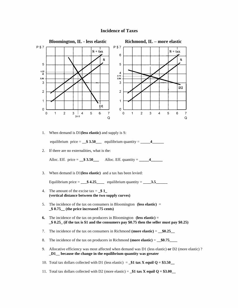
Incidence of Taxes
Bloomington, IL - less elastic Richmond, IL – more elastic
1. When demand is D1(less elastic) and supply is S:
equilibrium price = __$ 3.50___ equilibrium quantity = _____4______
2. If there are no externalities, what is the:
Alloc. Eff. price = __$ 3.50___ Alloc. Eff. quantity = _____4______
3. When demand is D1(less elastic) and a tax has been levied:
Equilibrium price = ___$ 4.25____ equilibrium quantity = ____3.5______
4. The amount of the excise tax = _$ 1_
(vertical distance between the two supply curves)
5. The incidence of the tax on consumers in Bloomington (less elastic) =
_$ 0.75__ (the price increased 75 cents)
6. The incidence of the tax on producers in Bloomington (less elastic) =
_$ 0.25_ (if the tax is $1 and the consumers pay $0.75 then the seller must pay $0.25)
7. The incidence of the tax on consumers in Richmond (more elastic) = __$0.25__
8. The incidence of the tax on producers in Richmond (more elastic) = __$0.75____
9. Allocative efficiency was most affected when demand was D1 (less elastic) or D2 (more elastic) ?
_D1__ because the change in the equilibrium quantity was greater
10. Total tax dollars collected with D1 (less elastic) = _$1 tax X equil Q = $3.50__
11. Total tax dollars collected with D2 (more elastic) = _$1 tax X equil Q = $3.00__
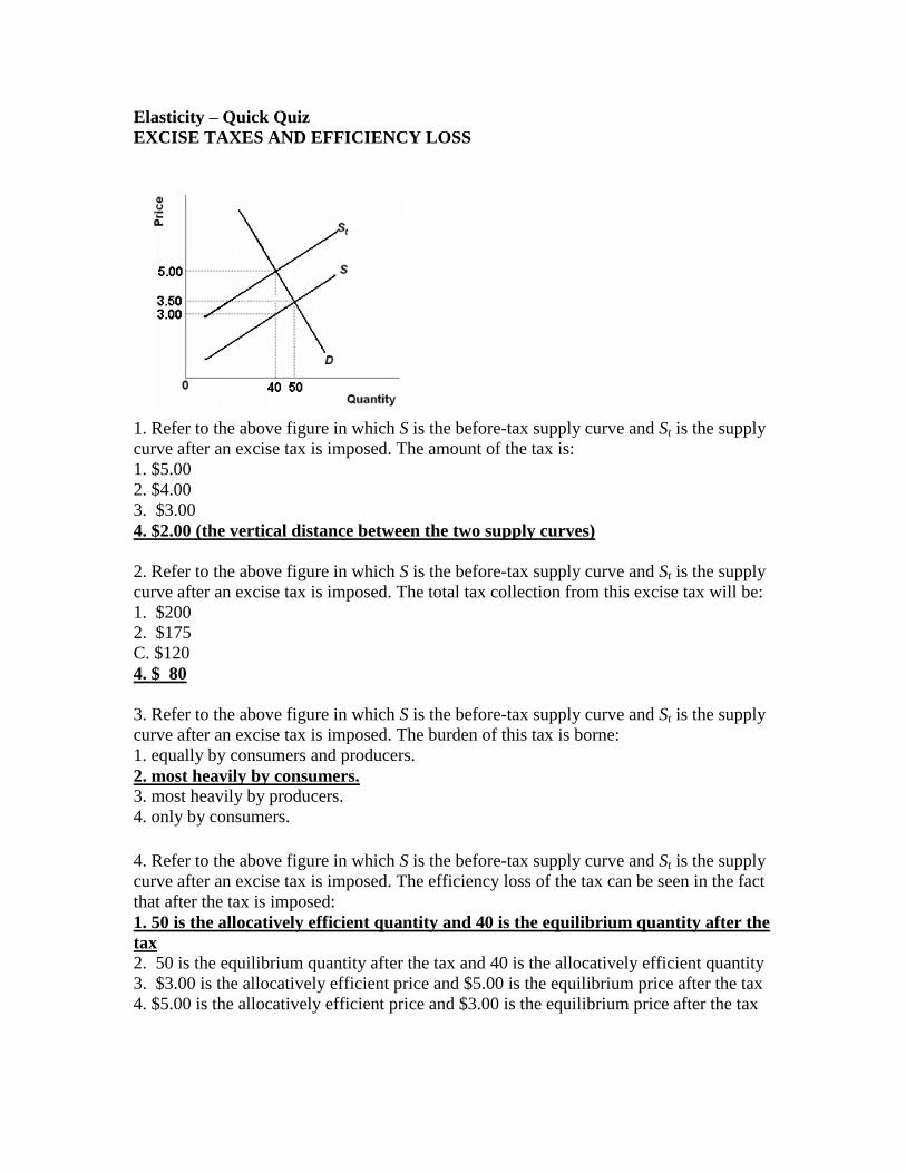
Elasticity – Quick Quiz
EXCISE TAXES AND EFFICIENCY LOSS
1. Refer to the above figure in which S is the before-tax supply curve and St is the supply
curve after an excise tax is imposed. The amount of the tax is:
1. $5.00
2. $4.00
3. $3.00
4. $2.00 (the vertical distance between the two supply curves)
2. Refer to the above figure in which S is the before-tax supply curve and St is the supply
curve after an excise tax is imposed. The total tax collection from this excise tax will be:
1. $200
2. $175
C. $120
4. $ 80
3. Refer to the above figure in which S is the before-tax supply curve and St is the supply
curve after an excise tax is imposed. The burden of this tax is borne:
1. equally by consumers and producers.
2. most heavily by consumers. 3. most heavily by producers.
4. only by consumers.
4. Refer to the above figure in which S is the before-tax supply curve and St is the supply
curve after an excise tax is imposed. The efficiency loss of the tax can be seen in the fact
that after the tax is imposed:
1. 50 is the allocatively efficient quantity and 40 is the equilibrium quantity after the
tax 2. 50 is the equilibrium quantity after the tax and 40 is the allocatively efficient quantity
3. $3.00 is the allocatively efficient price and $5.00 is the equilibrium price after the tax
4. $5.00 is the allocatively efficient price and $3.00 is the equilibrium price after the tax
5. The incidence of a tax pertains to:
1. the degree to which it alters the distribution of income.
2. how easy it is to evade the tax.
3. who actually bears the burden of a tax. 4. the progressiveness or regressiveness of tax rates.
6. If the demand for a product is perfectly inelastic and the supply curve is upsloping, a
$1 excise tax per unit of output will:
1. raise price by less than $1.
2. raise price by more than $1.
3. raise price by $1. 4. lower price by $1.

Elasticity – Quick Quiz
PRICE ELASTICITY OF SUPPLY
1. Suppose the supply of product X is perfectly inelastic. If there is an increase in the
demand for this product, equilibrium price:
1. will decrease but equilibrium quantity will increase.
2. and quantity will both decrease.
3. will increase but equilibrium quantity will decline.
4. will increase but equilibrium quantity will be unchanged.
2. Suppose that the price of product X rises by 20 percent and the quantity supplied of X
increases by 15 percent. The coefficient of price elasticity of supply for good X is:
1. negative and therefore X is an inferior good.
2. positive and therefore X is a normal good.
3. less than 1 and therefore supply is inelastic. 4. more than 1 and therefore supply is elastic.
3. Price elasticity of supply is:
1. positive in the short run but negative in the long run.
2. greater in the long run than in the short run. 3. greater in the short run than in the long run.
4. independent of time.
4. The supply of known Monet paintings is:
1. perfectly elastic.
2. perfectly inelastic. 3. relatively elastic.
4. relatively inelastic.

Elasticity – Quick Quiz
INCOME AND CROSS ELASTICITY
1. Suppose the income elasticity of demand for toys is +2.00. This means that:
1. a 10 percent increase in income will increase the purchase of toys by 20 percent. 2. a 10 percent increase in income will increase the purchase of toys by 2 percent.
3. a 10 percent increase in income will decrease the purchase of toys by 2 percent.
4. toys are an inferior good.
2. The formula for cross elasticity of demand is percentage change in:
1. quantity demanded of X/percentage change in price of X.
2. quantity demanded of X/percentage change in income.
3. quantity demanded of X/percentage change in price of Y. 4. price of X/percentage change in quantity demanded of Y.
3. Which type of goods is most adversely affected by recessions?
1. Goods for which the income elasticity coefficient is relatively low.
2. Goods for which the income elasticity coefficient is relatively high. 3. Goods for which the cross-price elasticity coefficient is positive.
4. Goods for which the cross-price elasticity coefficient is negative.
4. Cross elasticity of demand measures how sensitive purchases of a specific product are
to changes in:
1. the price of some other product. 2. the price of that same product.
3. income.
4. the general price level.
5. We would expect the cross elasticity of demand between Pepsi and Coke to be:
1. positive, indicating normal goods.
2. positive, indicating inferior goods.
3. positive, indicating substitute goods. 4. negative, indicating substitute goods.
6. Suppose that a 20 percent increase in the price of good Y causes a 10 percent decline
in the quantity demanded of good X. The coefficient of cross elasticity of demand is:
1. negative and therefore these goods are substitutes.
2. negative and therefore these goods are complements. 3. positive and therefore these goods are substitutes.
4. positive and therefore these goods are complements.

ELASTICITY WORKSHEET
1. Use the graph below for the question that follows.
Assume that the current price is $70. The seller wants to increase its revenues and has
decided to increase the price to $80. Is this a good idea?
It is a good idea ONLY IF demand is price inelastic (if the coefficient is less than 1),
because if demand is price inelastic and the price increases, then the total revenues
will increase. (If demand in elastic and the price increases the total revenue will go
down). So you have to calculate the coefficient of price elasticity of demand.
P1 = $ 70; Q1 = 40 and P2 = $ 80; Q2 = 30
-10 / 35
Ed = -------------- = .286 / .133 = 2.2
10 / 75
NO, they should not increase the price. Since Ed > 1, demand is price elastic and if
they raise the price their total revenues will go down.
-----------------------------------------------------------------------------------------------------------

2. Based on the determinants of elasticity as discussed in the text, guess what the price
elasticity of demand of the following products would be (elastic or inelastic?) and state
which determinant supports your guess.
(a) ballpoint pens – inelastic(?)
Number of Substitutes: many, so demand is more elastic
Product Price as a Proportion of Income: small, so demand is less elastic
Luxuries or Necessities: I don’t know if this really applies
Overall, I am not really sure. I would guess that demand is inelastic. If the
price goes up, I don’t think many people will cut back a lot on their
purchases of ballpoint pens.
(b) Crest toothpaste -- Elastic
Number of Substitutes: many, so demand is more elastic. All of the other
brands of toothpaste are substitutes for Crest brand.
Product Price as a Proportion of Income: small, so demand is less elastic
Luxuries or Necessities: Crest brand toothpaste is not a necessity, so demand is
more elastic
The demand for Crest toothpaste is probably price elastic since there are
many other brands to substitute for Crest, but the demand for toothpaste in
general is probably inelastic.
(c) diamond rings -- Elastic
Number of Substitutes: many, so demand is more elastic
Product Price as a Proportion of Income: large, so demand is more elastic
Luxuries or Necessities: luxury, so demand is more elastic
(d) sugar -- Inelastic
Number of Substitutes: few, so demand is less elastic
Product Price as a Proportion of Income: small, so demand is less elastic
Luxuries or Necessities: necessity, so demand is less elastic
(e) refrigerators -- Inelastic
Number of Substitutes: few, so demand is less elastic
Product Price as a Proportion of Income: somewhat large, so maybe demand is
more elastic
Luxuries or Necessities: necessity so demand is less elastic

3. Use the information in the table below to identify the type of cross elasticity
relationship between products X and Y and whether demand is cross elastic or cross
inelastic in each of the following five cases, A to E.
Percent change
Percent change in quantity Substitute or Cross Elastic
Cases in price of Y demanded of X Complement? or Inelastic?
A 5 7 substitutes 7/5 > 1, elastic
B –9 –6 substitutes 6/9 <1, inelastic
C 5 –5 complements = 1, unit elastic
D 3 0 independent ____0______
E –2 10 complements 10/2 > 1. elastic
If the coefficient of cross elasticity of demand is + then the products are
substitutes.
If the coefficient of cross elasticity of demand is + then the products are
complements.
If the coefficient of cross elasticity of demand is 0 then the products are
independent goods.
4. Use the information in the table below to identify the income elasticity type of each of
the following products, A to E.
% change Normal elastic,
% change in quantity or inelastic,
Product in income demanded Inferior or unit elastic
A 9 12 normal good 12/9 > 1, elastic
B –6 6 inferior good 6/6 = 1, unit elastic
C 3 3 normal good 3/3 = 1, unit elastic
D 6 –3 inferior good 3/6 < 1, inelastic
E –2 –1 normal good 1/2 < 1, inelastic
If the coefficient of income elasticity of demand is + then the products are
normal goods.
If the coefficient of income elasticity of demand is + then the products are
inferior goods.
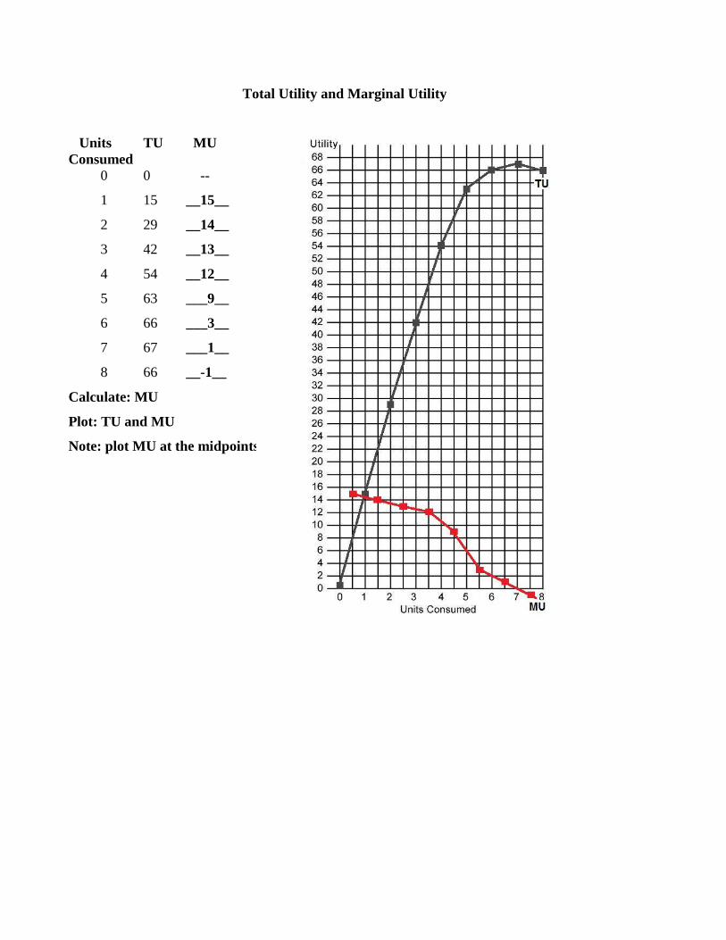
Total Utility and Marginal Utility
Units TU MU
Consumed
0 0 --
1 15 __15__
2 29 __14__
3 42 __13__
4 54 __12__
5 63 ___9__
6 66 ___3__
7 67 ___1__
8 66 __-1__
Calculate: MU
Plot: TU and MU
Note: plot MU at the midpoints

Utility Maximizing Rule
You have $10
The price of beer is $1 per bottle
The price of a steak sandwich is $3
The utility received from consuming beer and steak is given below.
PROBLEM: How many beers and steak sandwiches should be bought to maximize utility?
Number
of
Beers
TU
beer
MU
beer
MU/P
beer
Number
of
Steaks
TU
steaks
MU
steaks
MU/P
steaks
0 0 -- -- 0 0 -- --
1 15 15 15 1 24 24 8
2 24 9 9 2 45 21 7
3 32 8 8 3 63 18 6
4 39 7 7 4 75 12 4
6 45 6 6 5 84 9 3
7 47 2 2 6 87 3 1
Calculate utility maximizing quantities of beer and steak sandwiches when income equals
$10 and the price of beer is $1 and the price of steak sandwiches is $3 using the utility maximizing rule.
You have $10 to spend. You should spend your money on the product that gives you the most satisfaction per
dollar (MU/P). So when the waitress comes to the table what do you buy first on beer or one steak? Since the
beer gives you 15 units of satisfaction per dollar and the steak gives you only 8 per dollar, buy the first beer.
What do you buy next? Since the second beer gives you 9 units of satisfaction per dollar (MU/P) and the first
steak gives you only 8, you should buy another beer. Next you should buy one of each since they both give 8
units of satisfaction per dollar.
How much have you spent? So far you have bought three beers for $1 each and one steak for $3 which is a
total of $6. Since you have $10 what do you buy next? You should buy the fourth beer and the second steak
since they both give you 7 units of satisfaction per dollar.
What do you buy next? Nothing, because you have spent your $10 and you are out of money.
So to maximize your utility you should buy 4 beers and 2 steak sandwiches.
Calculate the TOTAL UTILITY received.
4 beers give you 39 units of satisfactions and 2 steaks give you 45 for a total of 84. There is no other
combination of beer and steak that you can buy with your $10 that will give you more satisfaction. Try it.
You could afford 1 beer and 3 steaks and you can afford 7 beers and 1 steak. If you calculate the total utility
received from these combinations it will be less than the 84 that you got from 4 beers and 2 steaks.
CHAPTER 7: REVIEW -Consumer Behavior and Utility Maximization
What is UTILITY?
The want-satisfying power of a good or service; the satisfaction or pleasure a consumer obtains
from the consumption of a good or service (or from the consumption of a collection of goods and
services).
Define MARGINAL UTILITY and give its FORMULA.
The extra utility a consumer obtains from the consumption of one additional unit of a good or
service;
equal to the change in total utility divided by the change in the quantity consumed.
MU = TU / Qconsumed
What is the LAW OF DIMINISHING MARGINAL UTILITY?
As a consumer increases the consumption of a good or service the marginal utility obtained from
each additional unit of the good or service decreases.
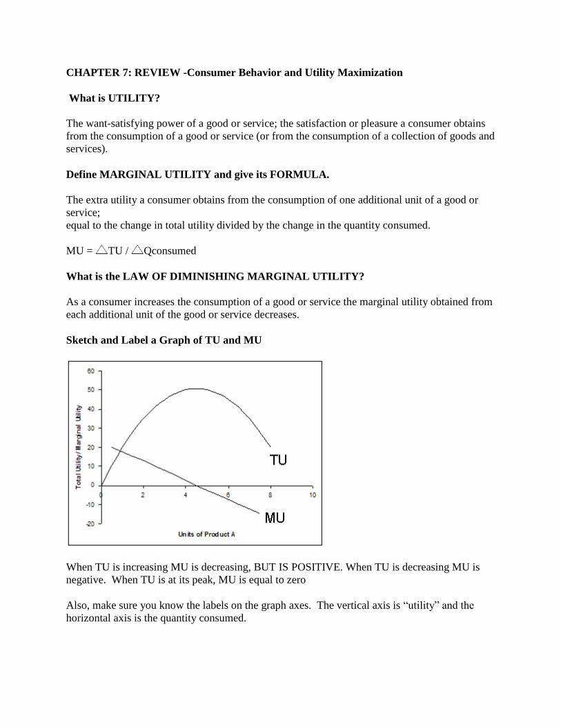
Sketch and Label a Graph of TU and MU
When TU is increasing MU is decreasing, BUT IS POSITIVE. When TU is decreasing MU is
negative. When TU is at its peak, MU is equal to zero
Also, make sure you know the labels on the graph axes. The vertical axis is “utility” and the
horizontal axis is the quantity consumed.

Can utility be measured?
No, utility cannot be measured, but it can be compared. I know that I like Butterfinger candy
bars more than Snickers candy bars, but I can’t how much utility I get from a Butterfinger candy
bar.

Write the Benefit-Cost Analysis formula
select all where: MB > MC
up to where: MB = MC
but never where: MB < MC
MB = MC
Write the utility maximizing rule formula
MUx / Px = MUy / Py = MUz/Pz
Explain why the utility maximizing rule is really a version of Benefit-Cost Analysis.
According to benefit-cost analysis the best answer is where MB = MC
The marginal benefit that we receive from consuming one more dollar’s worth of product x is:
MBx = MUx/Px The MB of product X can be measured by finding the MU per dollar spent on
product X. The MC of product X can be measured by finding the MU that you are not receiving
from a dollar's worth of your next best alternative (product Y): MCx = MUy/Py
Therefore: MB = MC or MUx / Px = MUy / Py
To obtain the greatest utility the consumer should allocate money income so that the last dollar
spent on each good or service yields the same marginal utility.

PROBLEM 1
Assume that a consumer purchases a combination of products A and B. The MUa is 5 and
the Pa is $5. The MUb is 6 and the Pb is $6.
What should this consumer do to maximize utility?
To maximize utility we use the utility maximizing rule:
MUa / Pa = MUb / Pb
The MUa /Pa = 1. The MUb /Pb = 1. The consumer is maximizing utility and should make no
changes in consumption patterns. The marginal utility per dollar is the same for both products.
PROBLEM 2
Assume that a consumer purchases a combination of products Y and Z. The MUy is 50 and
the Py is $25. The MUz is 20 and the Pz is $5.
What should this consumer do to maximize utility?
To maximize utility we use the utility maximizing rule:
MUy / Py = MUz / Pz
The MUy/Py = 2. The MUz/Pz = 4. The consumer should consume more of product Z and less
of product Y until the marginal utility per dollar is the same for both products

PROBLEM 3
Columns 1 through 3 in the table below show the marginal utility which a particular
consumer would get by purchasing various quantities of products a, b, and c.
Qa MUa MUa/Pa
Qb MUb MUb/Pb Qc MUc MUc/Pc
1 18 9 1 39 13 1 12 12
2 16 8 2 36 12 2 10 10
3 14 7 3 33 11 3 9 9
4 12 6 4 30 10 4 8 8
5 10 5 5 27 9 5 7 7
7 8 4 6 24 8 6 5 5
7 6 3 7 21 7 7 3 3
If the prices of a, b, and c are $2, $3, and $1, respectively, and the consumer has $26 to
spend on these three products, what combination of the three products should be
purchased in order to maximize utility and what is the maximum utility possible?
To maximize utility we use the utility maximizing rule:
MUa / Pa = MUb / Pb = MUc/Pc
So the first thing you have to do is calculate the MU/P = marginal utility per dollar
Then “go shopping” and buy each product in order of which one gives you the most
MU for each dollar that you spend. What do you buy first? The first b gives you 13
units of satisfaction per dollar which is more than the first a or c. So buy one b.
What do you buy next? The second b and the first c both give 12 units of satisfaction
per dollar, so buy them. What do you buy next? The third b since it gives more
satisfaction per dollar (11) than the others.
Keep shopping until you have spent all of your money ($26). The end result will be 2
units of a, 6 units of b, and 4 units of c.
To get the maximum utility possible you must add up all of the marginal utilities.
For a: 18 + 16
For b: 39 + 36 + 33 + 30 + 27 + 24
For c: 12 + 10 + 9 + 8
Total: 262 units of satisfaction is the maximum possible given the data.

Quick Quiz
CONSUMER BEHAVIOR
1. Refer to the above data. The value for Y is:
1. 25.
2. 30.
3. 40.
4. 45.
2. Refer to the above data. The value for X is:
1. 15. 2. 5.
3. 55.
4. 10.
3. Refer to the above data. The value for W is:
1. 15.
2. 20. 3. 25.
4. 30.
4. Refer to the above data. The value for Z is:
1. -5. 2. +5.
3. -10.
D. zero.
5. Marginal utility is the:
1. sensitivity of consumer purchases of a good to changes in the price of that good.
2. change in total utility obtained by consuming one more unit of a good. 3. change in total utility obtained by consuming another unit of a good divided by the change in
the price of that good.
4. total utility associated with the consumption of a certain number of units of a good divided by
the number of units consumed.

6. Where total utility is at a maximum, marginal utility is:
1. negative.
2. positive and increasing.
3. zero. 4. positive but decreasing.
7. Newspapers dispensing devices seemingly "trust" people to take only a single paper but the
devices actually rely on the law of:
1. supply.
2. increasing opportunity costs.
3. demand.
4. diminishing marginal utility.
8. Suppose that Ms. Thomson is currently exhausting her money income by purchasing 10 units
of A and 8 units of B at prices of $2 and $4 respectively. The marginal utility of the last units of
A and B are 16 and 24 respectively. These data suggest that Ms. Thomson:
1. has preferences that are at odds with the principle of diminishing marginal utility.
2. considers A and B to be complementary goods.
3. should buy less A and more B.
D. should buy less B and more A.
9. Refer to the above data. Assume the price of X is $2 and the price of Y is $1 and there is a
total of $9 to spend. What quantities of X and Y should be purchased to maximize utility?
1. 2 of X and 1 of Y
2. 4 of X and 5 of Y
3. 2 of X and 5 of Y 4. 2 of X and 6 of Y
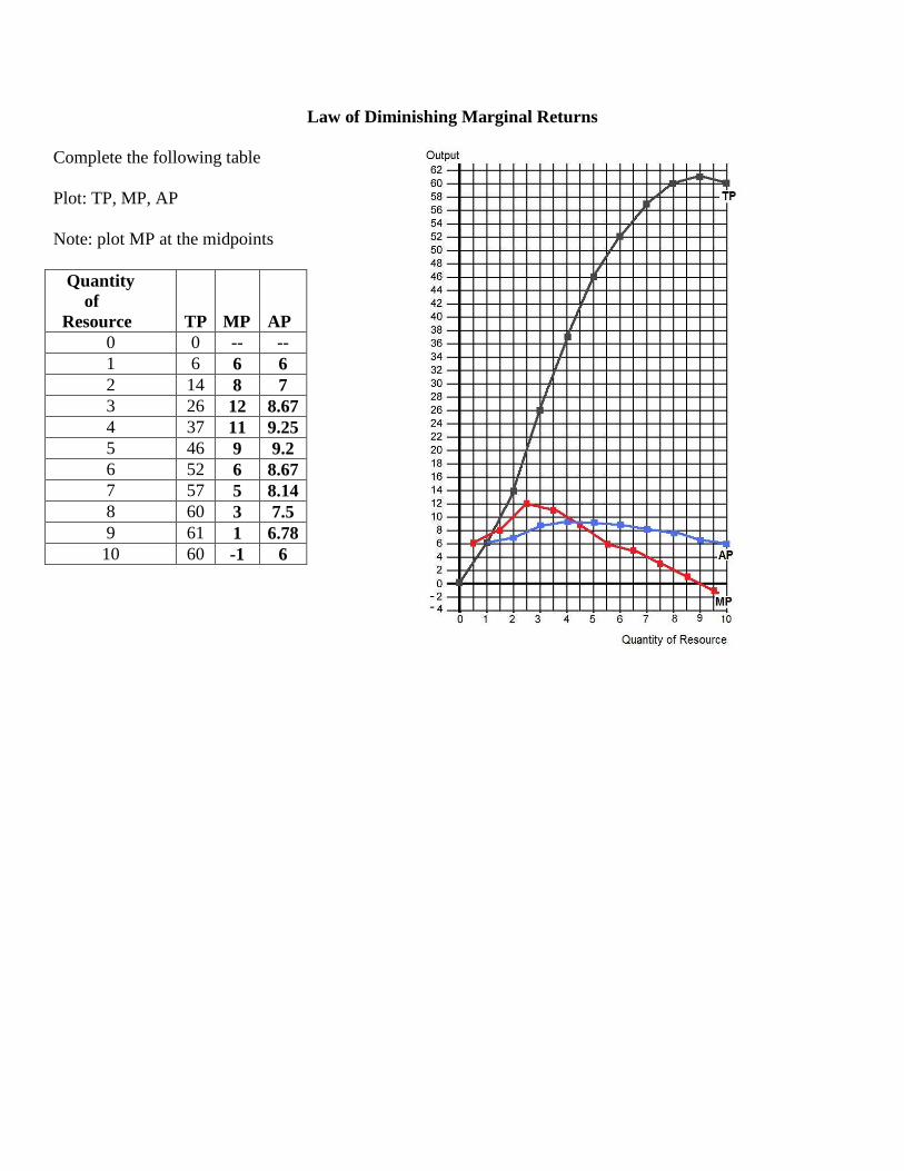
Law of Diminishing Marginal Returns
Complete the following table
Plot: TP, MP, AP
Note: plot MP at the midpoints
Quantity
of
Resource
TP
MP
AP
0 0 -- --
1 6 6 6
2 14 8 7
3 26 12 8.67
4 37 11 9.25
5 46 9 9.2
6 52 6 8.67
7 57 5 8.14
8 60 3 7.5
9 61 1 6.78
10 60 -1 6

Costs of Production – Quick Quiz
PRODUCTION FUNCTION
1. Accounting profits are typically:
1. greater than economic profits because the former do not take explicit costs into account.
2. equal to economic profits because accounting costs include all opportunity costs.
3. smaller than economic profits because the former do not take implicit costs into account.
4. greater than economic profits because the former do not take implicit costs into account.
2. Suppose that a business incurred implicit costs of $200,000 and explicit costs of $1 million in
a specific year. If the firm sold 4,000 units of its output at $300 per unit, its accounting profits
were:
1. $100,000 and its economic profits were zero.
2. $200,000 and its economic profits were zero. 3. $100,000 and its economic profits were $100,000.
4. zero and its economic loss was $200,000.
3. The basic characteristic of the short run is that:
1. barriers to entry prevent new firms from entering the industry.
2. the firm does not have sufficient time to change the size of its plant. 3. the firm does not have sufficient time to cut its rate of output to zero.
4. a firm does not have sufficient time to change the amounts of any of the resources it employs.
4. Which of the following represents a long-run adjustment?
1. a farmer uses an extra dose of fertilizer on his corn crop
2. unable to meet foreign competition, a U.S. watch manufacturer sells one of its branch
plants 3. a steel manufacturer cuts back on its purchases of coke and iron ore
4. a supermarket hires four additional clerks
5. If in the short run a firm's total product is increasing, then its:
1. marginal product must also be increasing.
2. marginal product must be decreasing.
3. marginal product could be either increasing or decreasing. 4. average product must also be increasing.
6. The law of diminishing returns describes the:
1. relationship between total costs and total revenues.
2. profit-maximizing position of a firm.
3. relationship between resource inputs and product outputs in the short run. 4. relationship between resource inputs and product outputs in the long run.

Answer the next question(s) on the basis of the following output data for a firm. Assume that the
amounts of all non-labor resources are fixed.
7. Refer to the above data. Diminishing marginal returns become evident with the addition of
the:
1. sixth worker.
2. fourth worker.
3. third worker. 4. second worker.
8. When total product is increasing at a decreasing rate, marginal product is:
1. positive and increasing.
2. positive and decreasing. 3. constant.
4. negative.

Short-Run Cost Schedules and Curves
Q TFC TVC TC AFC AVC ATC MC
0 $ 25 $ 0 $ 25 $ -- $ -- $ -- $ --
1 25 10 35 25 10.00 35 10
2 25 16 41 12.50 8.00 20.50 6
3 25 20 45 8.33 6.67 15.00 4
4 25 22 47 6.25 5.50 11.75 2
5 25 24 49 5.00 4.80 9.80 2
6 25 27 52 4.17 4.50 8.67 3
7 25 32 57 3.57 4.57 8.14 5
8 25 40 65 3.125 5.00 8.125 8
9 25 54 79 2.78 6.00 8.78 14
10 25 75 100 2.50 7.50 10.00 21
Plot: ATC, AVC, and MC
Plot: TC, TVC, and TFC

Plot: ATC, AVC, and MC
Plot: TC, TVC, and TFC

REVIEW – Short Run Costs
(a) How can you tell if these cost curves are
for the short run or the long run?
The ATC, AVC, and MC curves are for one
size of plant. In the short run, there are fixed
costs and variable costs. In the long run, all
costs are variable.
So since you see both ATC and AVC it means
that you must have some fixed costs and
therefore these are short run curves.
(b)
(1) AVC at 6,000 units is $4.00.
(2) ATC at 6,000 units is $5.50.
(3) AFC at 6,000 units is $1.50.
(4) TVC at 6,000 units is $24,000 ($4.00 x 6,000).
(5) TFC at all levels of output is $9,000.
(6) TC at 6,000 units is $33,000.
(7) Diminishing marginal returns set in at 3,000 units.
(4) TVC at 6,000 units of output and show on
graph?
(6) TC at 6,000 units of output and show on
graph?
(5) TFC at all levels of output and show on
graph?
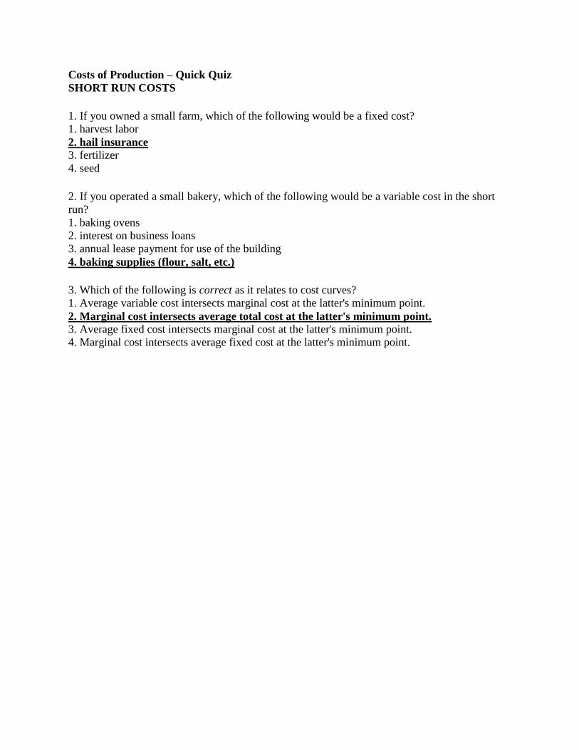
Costs of Production – Quick Quiz
SHORT RUN COSTS
1. If you owned a small farm, which of the following would be a fixed cost?
1. harvest labor
2. hail insurance 3. fertilizer
4. seed
2. If you operated a small bakery, which of the following would be a variable cost in the short
run?
1. baking ovens
2. interest on business loans
3. annual lease payment for use of the building
4. baking supplies (flour, salt, etc.)
3. Which of the following is correct as it relates to cost curves?
1. Average variable cost intersects marginal cost at the latter's minimum point.
2. Marginal cost intersects average total cost at the latter's minimum point.
3. Average fixed cost intersects marginal cost at the latter's minimum point.
4. Marginal cost intersects average fixed cost at the latter's minimum point.

4. Refer to the above diagram. At output level Q total variable cost is:
1. 0BEQ. 2. BCDE.
3. 0CDQ.
4. 0AFQ.
5. Refer to the above diagram. At output level Q total fixed cost is:
1. 0BEQ.
2. BCDE. 3. 0BEQ - 0AFQ.
4. 0CDQ.
6. Refer to the above diagram. At output level Q total cost is:
1. 0BEQ.
2. BCDE.
3. 0BEQ plus BCDE. 4. 0AFQ plus BCDE.
7. Refer to the above diagram. At output level Q average fixed cost:
1. is equal to EF.
2. is equal to QE.
3. is measured by both QF and ED. 4. cannot be determined from the information given.
8. Refer to the above diagram. At output level Q:
1. marginal product is falling. 2. marginal product is rising.
3. marginal product is negative.
4. one cannot determine whether marginal product is falling or rising.

Answer the next question(s) on the basis of the following cost data:
9. Refer to the above data. The total variable cost of producing 5 units is:
1. $61.
2. $48.
3. $37. 4. $24.
10. Refer to the above data. The average total cost of producing 3 units of output is:
1. $14.
2. $12.
3. $13.50.
4. $16.
11. Refer to the above data. The average fixed cost of producing 3 units of output is:
1. $8. 2. $7.40.
3. $5.50.
4. $6.
12. Refer to the above data. The marginal cost of producing the sixth unit of output is:
1. $24.
2. $12.
3. $16.
4. $8.

Costs of Production – Quick Quiz
LONG RUN COSTS
1. Economies and diseconomies of scale explain:
1. the profit-maximizing level of production.
2. why the firm's long-run average total cost curve is U-shaped. 3. why the firm's short-run marginal cost curve cuts the short-run average variable cost curve at
its minimum point.
4. the distinction between fixed and variable costs.
2. In the long run:
1. all costs are variable costs. 2. all costs are fixed costs.
3. variable costs equal fixed costs.
4. fixed costs are greater than variable costs.
3. The above diagram shows the short-run average total cost curves for five different plant sizes
of a firm. The shape of each individual curve reflects:
1. increasing returns, followed by diminishing returns. 2. economies of scale, followed by diseconomies of scale.
3. constant costs.
4. increasing costs, followed by decreasing costs.
4. As the firm in the above diagram expands from plant size #1 to plant size #3, it experiences:
1. diminishing returns.
2. economies of scale. 3. diseconomies of scale.
4. constant costs.

Use the following data to answer the next question(s). The letters A, B, and C designate three
successively larger plant sizes.
5. Refer to the above data. At what level of output is minimum efficient scale realized?
1. 30
2. 40
3. 50 4. 60
6. Economies of scale are indicated by:
1. the rising segment of the average variable cost curve.
2. the declining segment of the long-run average total cost curve. 3. the difference between total revenue and total cost.
4. a rising marginal cost curve.
7. If an industry's long-run average total cost curve has an extended range of constant returns to
scale, this implies that:
1. technology precludes both economies and diseconomies of scale.
2. the industry will be a natural monopoly.
3. both relatively small and relatively large firms can be viable in the industry.
4. the industry will be comprised of a very large number of small firms.
8. Diseconomies of scale arise primarily because:
1. the short-run average total cost curve rises when marginal product is increasing.
2. of the difficulties involved in managing and coordinating a large business enterprise. 3. firms must be large both absolutely and relative to the market to employ the most efficient
productive techniques available.
4. beyond some point marginal product declines as additional units of a variable resource (labor)
are added to a fixed resource (capital).

9. Refer to the above diagram. Minimum efficient scale:
1. occurs at some output greater than Q3.
2. is achieved at Q1. 3. is achieved at Q3.
4. cannot be identified in this diagram.
10. Suppose a firm is in a range of production where it is experiencing economies of scale.
Knowing this, we can predict that:
1. the long-run average total cost curve is upsloping.
2. a 10 percent increase in all inputs will increase output by less than 10 percent.
3. a 10 percent increase in all inputs will increase output by more than 10 percent. 4. the firm is encountering problems of managerial bureaucracy because of its size.