ECIV 720 A Advanced Structural

Mechanics and Analysis

Lecture 10: Solution of Continuous Systems –

Fundamental Concepts

• Mixed Formulations• Intrinsic Coordinate Systems

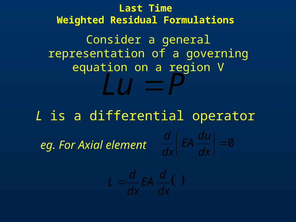
Last TimeWeighted Residual Formulations

Consider a general representation of a governing equation on a region V

PLu L is a differential operator

0

dx

duEA

dx

deg. For Axial element

dx

dEA

dx

dL

Last TimeWeighted Residual Formulations

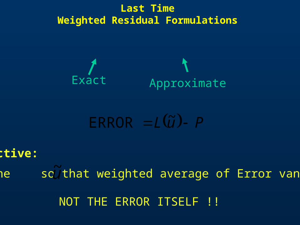
Exact Approximate

PuL ~ ERROR

Objective:

Define so that weighted average of Error vanishesu~

NOT THE ERROR ITSELF !!

Last TimeWeighted Residual Formulations

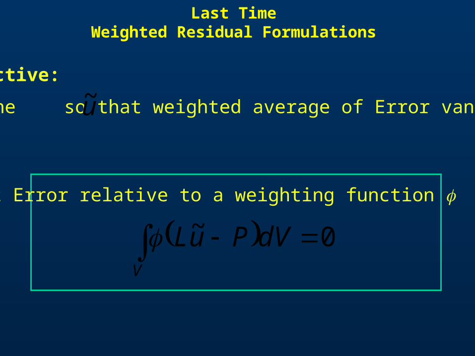
Set Error relative to a weighting function

0~ V

dVPuL

Objective:

Define so that weighted average of Error vanishesu~

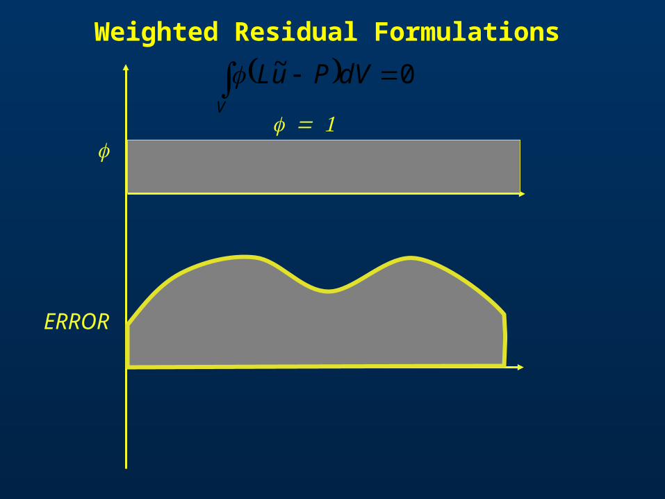
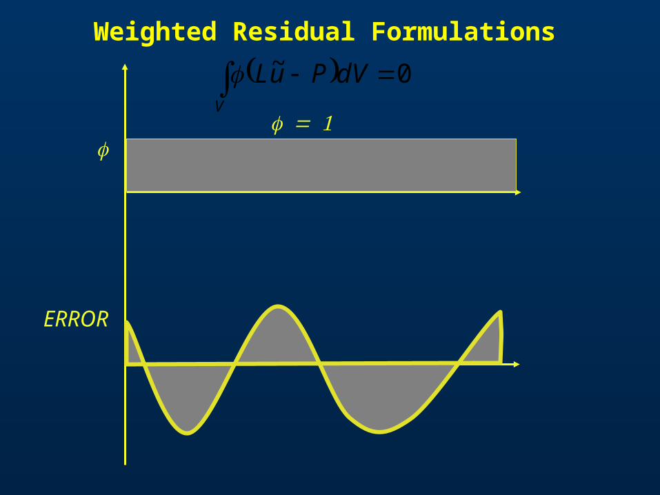
Weighted Residual Formulations

ERROR

0~ V

dVPuL

Weighted Residual Formulations

ERROR

0~ V

dVPuL

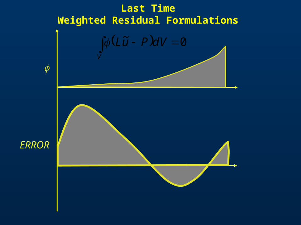
Last TimeWeighted Residual Formulations

ERROR

0~ V

dVPuL

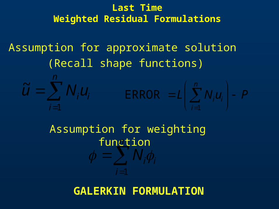
Last TimeWeighted Residual Formulations

Assumption for approximate solution

(Recall shape functions)

n

iiiuNu

1

~PuNL

n

iii

1

ERROR

Assumption for weighting function

n

iiiN

1

GALERKIN FORMULATION

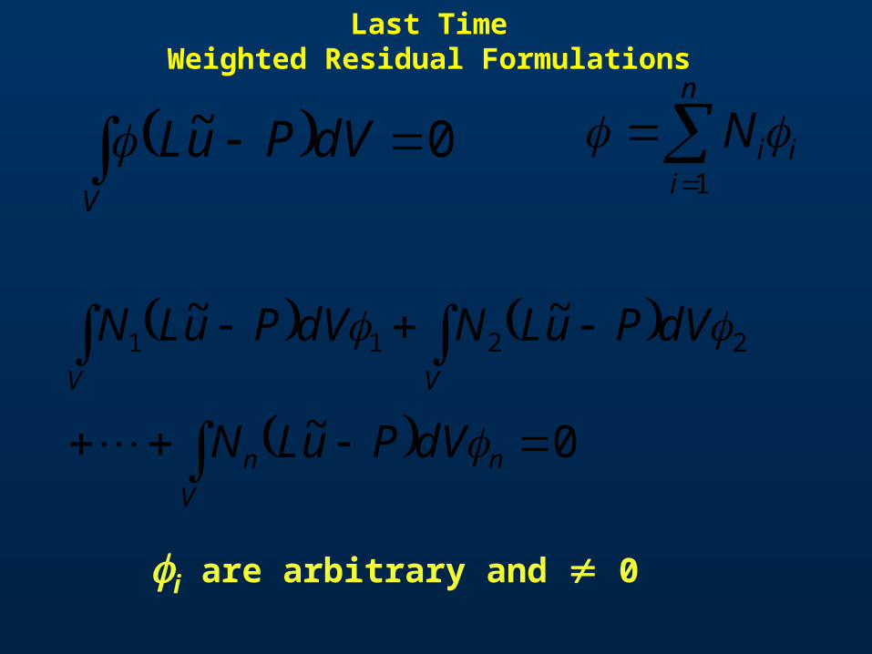
Last TimeWeighted Residual Formulations

0~

~~2211

n

V

n

VV

dVPuLN

dVPuLNdVPuLN

0~ V

dVPuL

n

iiiN

1

i are arbitrary and 0

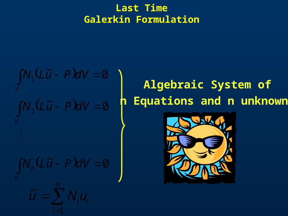
Last TimeGalerkin Formulation

Algebraic System of

n Equations and n unknowns

0~

1 V

dVPuLN

0~2

V

dVPuLN

0~ V

n dVPuLN

n

iiiuNu

1

~

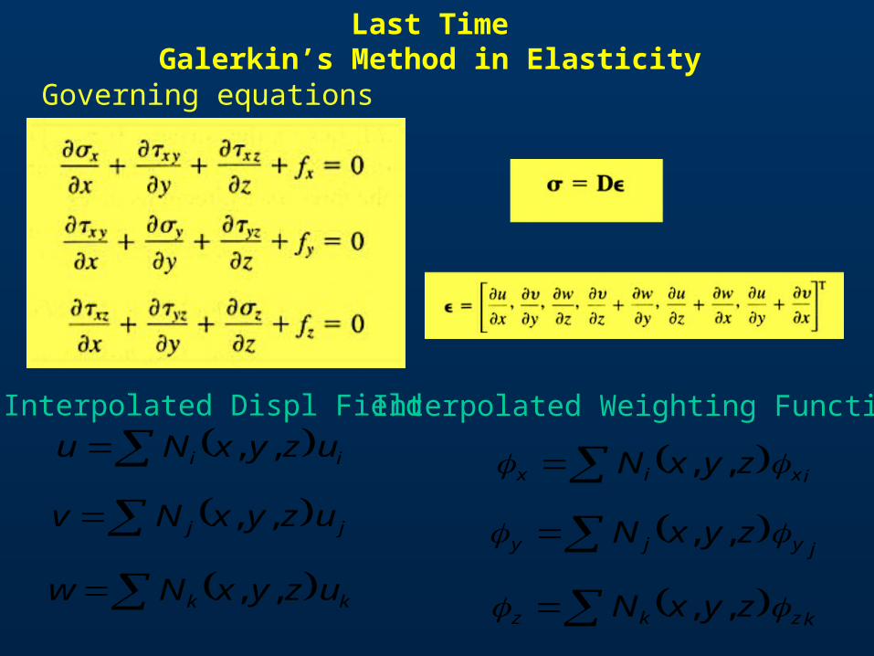
Last TimeGalerkin’s Method in Elasticity

Governing equations

Interpolated Displ Field

ii uzyxNu ,,

jj uzyxNv ,,

kk uzyxNw ,,

Interpolated Weighting Function

ixix zyxN ,,

jyjy zyxN ,,

kzkz zyxN ,,

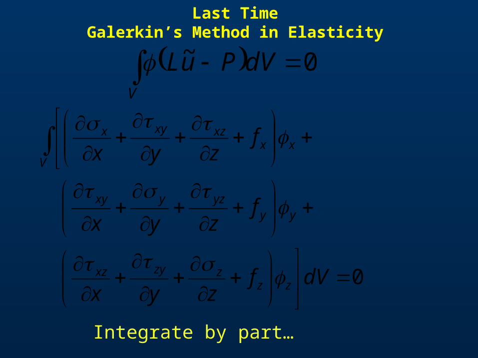
Last TimeGalerkin’s Method in Elasticity

0

dVfzyx

fzyx

fzyx

zzzzyxz

yyyzyxy

V

xxxzxyx

Integrate by part…

0~ V

dVPuL

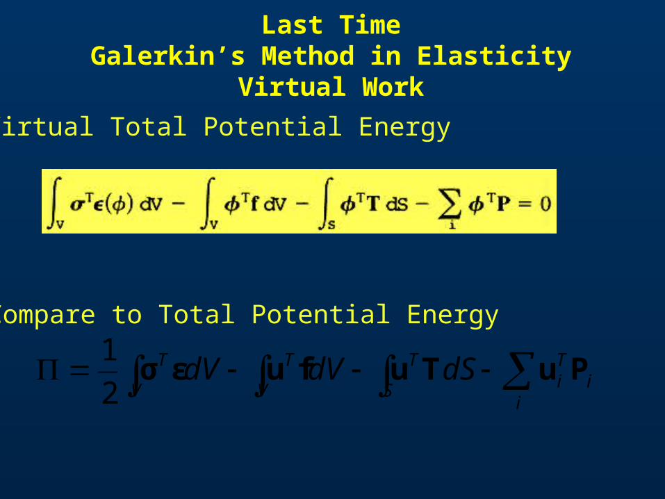
Last TimeGalerkin’s Method in Elasticity Virtual

Work

i

iTiS

T

V

T

V

T dSdVdV PuTufuεσ2

1

Compare to Total Potential Energy

Virtual Total Potential Energy

Last TimeGalerkin’s Formulation

•More general method

•Operated directly on Governing Equation

•Variational Form can be applied to other governing equations

•Preffered to Rayleigh-Ritz method especially when function to be minimized is not available.

Mixed Formulation

• Displacement Based FE approximations– Combine subsidiary equations to obtain G.E.– G.E. in terms of displacements– Stresses, Strains etc enter as natural B.C.

• Mixed Formulation– Apply Galerkin directly on subsidiary relations– Nodal dof contain displacements AND other field

quantities

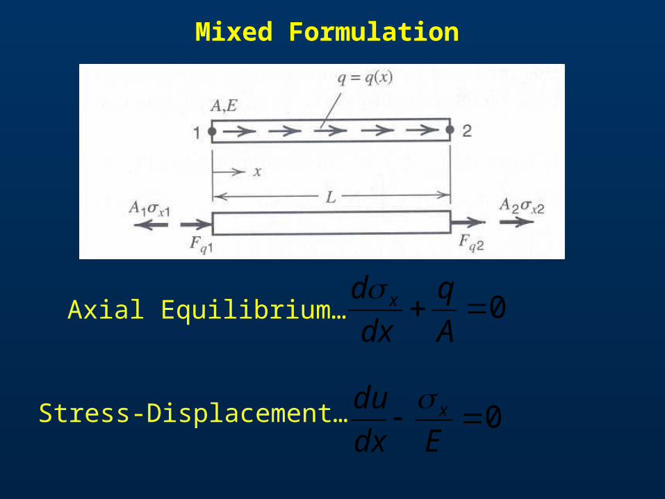
Mixed Formulation

0A

q

dx

d xAxial Equilibrium…

0Edx

du xStress-Displacement…

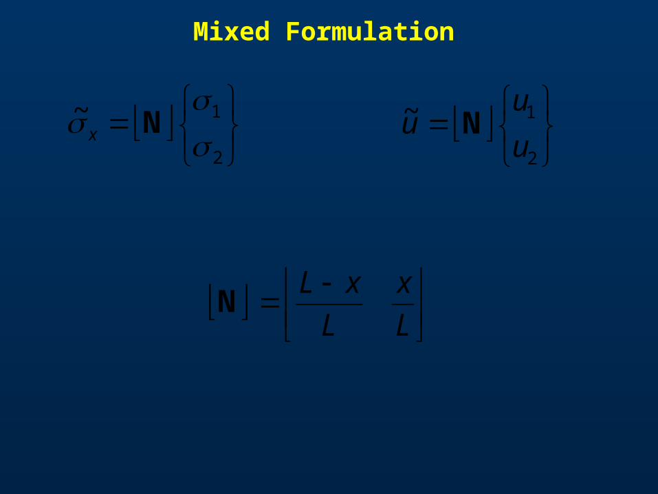
Mixed Formulation

2

1~

Nx

2

1~u

uu N

L

x

L

xLN

Mixed Formulation

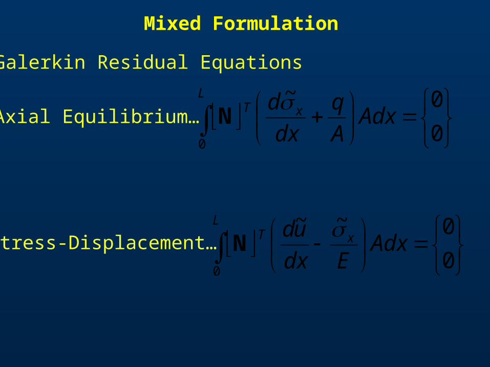
Galerkin Residual Equations

0

0~

0

LxT Adx

A

q

dx

dNAxial Equilibrium…

0

0~~

0

LxT Adx

Edx

ud NStress-Displacement…

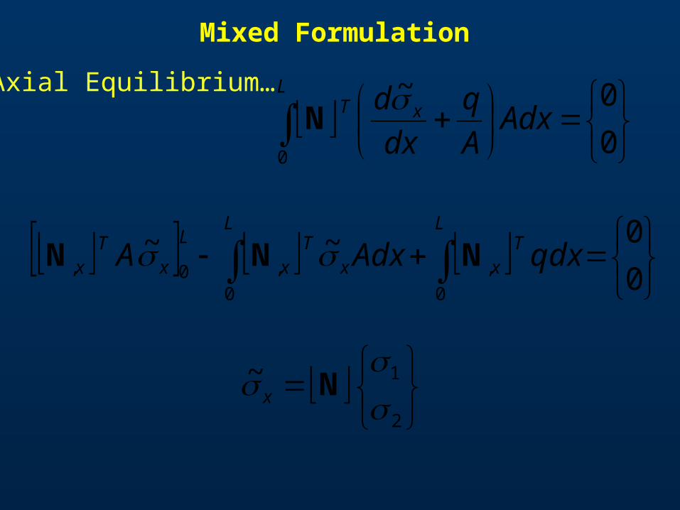
Mixed Formulation

0

0~

0

LxT Adx

A

q

dx

dN

Axial Equilibrium…

0

0~~

0

,

0

,0,

LT

x

L

xT

x

L

xT

x qdxAdxA NNN

2

1~

Nx

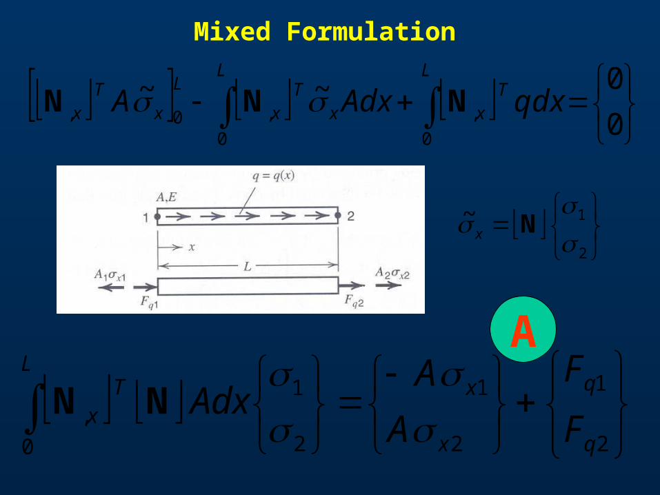
Mixed Formulation

2

1

2

1

2

1

0

,q

q

x

xL

Tx F

F

A

AAdx

NN

0

0~~

0

,

0

,0,

LT

x

L

xT

x

L

xT

x qdxAdxA NNN

2

1~

Nx

A

Mixed Formulation

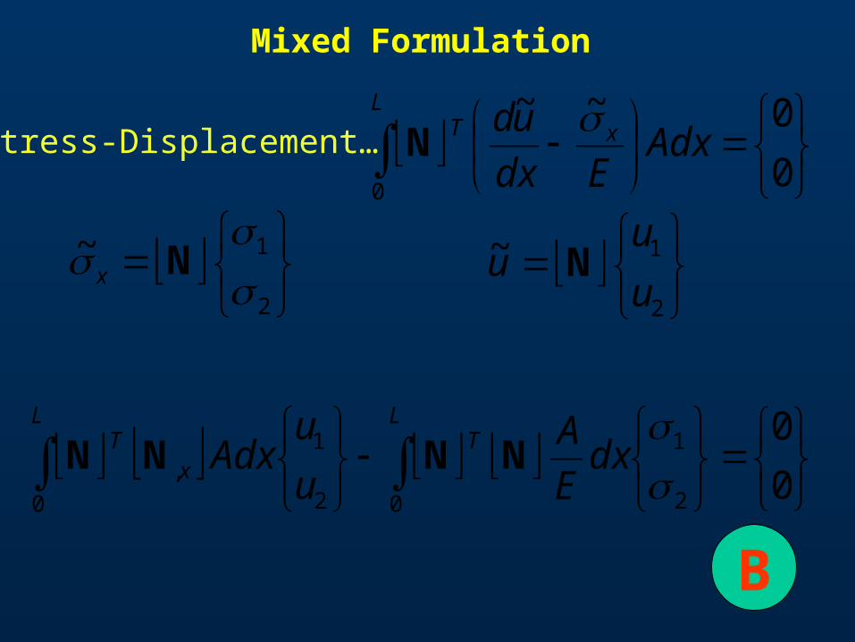
0

0~~

0

LxT Adx

Edx

ud NStress-Displacement…

2

1~

Nx

2

1~u

uu N

0

0

2

1

02

1

0

, L

TL

xT dx

E

A

u

uAdx NNNN

B

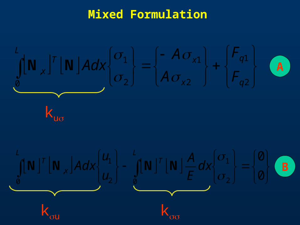
Mixed Formulation

2

1

2

1

2

1

0

,q

q

x

xL

Tx F

F

A

AAdx

NN

0

0

2

1

02

1

0

, L

TL

xT dx

E

A

u

uAdx NNNN

ku

ku k

A

B

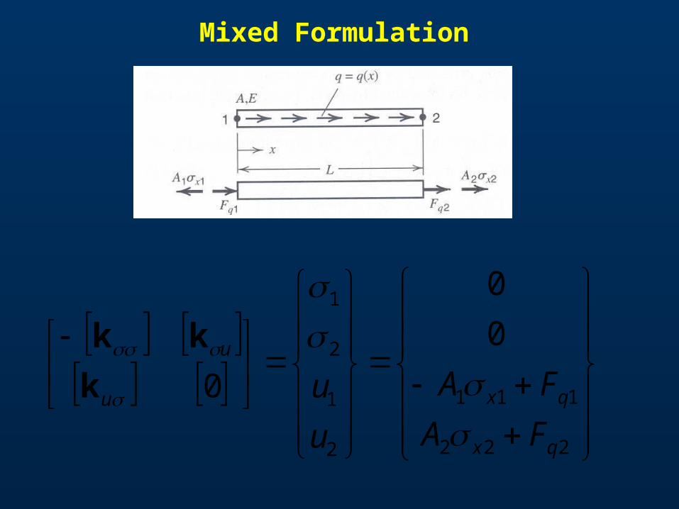
Mixed Formulation

222

111

2

1

2

1

0

0

0

qx

qxu

u

FA

FA

u

u

k

kk

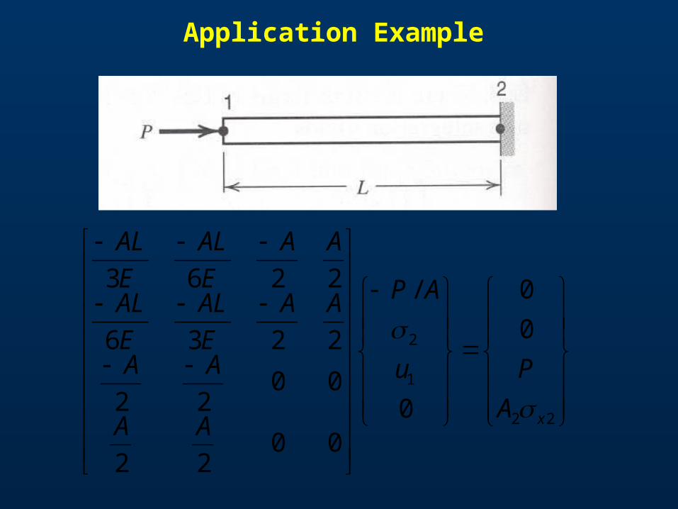
Application Example

22

1

2 0

0

0

/

0022

0022

2236

2263

xA

Pu

AP

AA

AA

AA

E

AL

E

AL

AA

E

AL

E

AL

INTRINSIC COORDINATE SYSTEMS

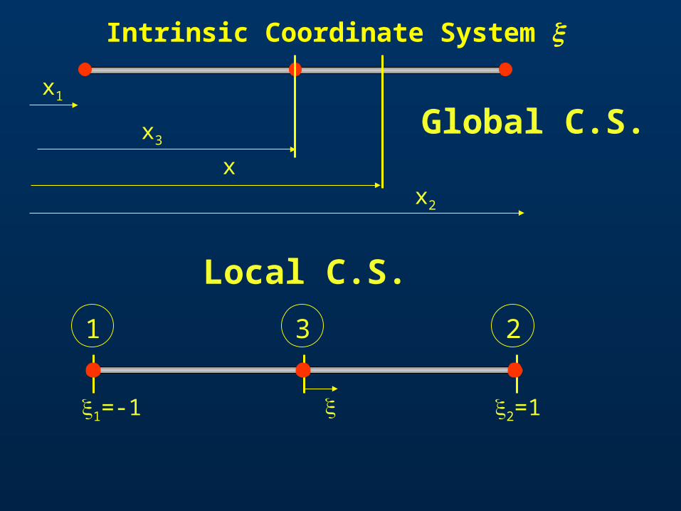
Intrinsic Coordinate System

x1

xx2

x3

1=-1

1

3

2=1

2

Global C.S.

Local C.S.

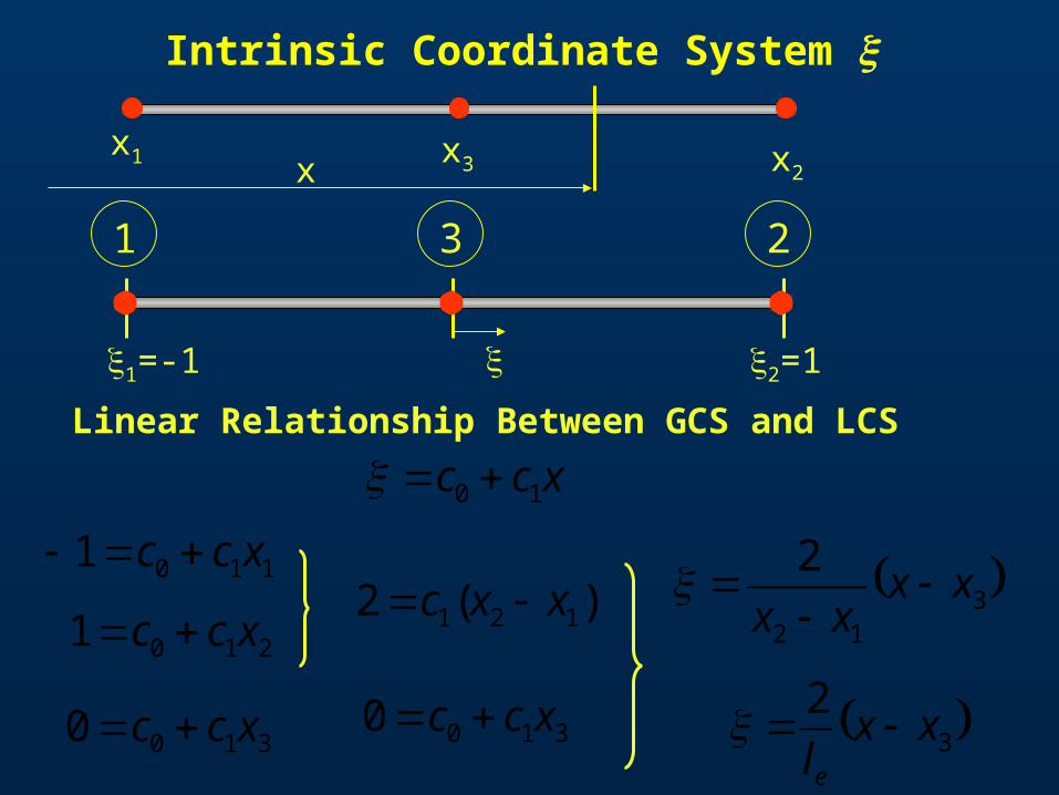
Intrinsic Coordinate System

x1 x x2x3

1=-1

1

3

2=1

2

312

2xx

xx

Linear Relationship Between GCS and LCS

xcc 10

1101 xcc

2101 xcc

3100 xcc

)(2 121 xxc

3100 xcc 3

2xx

le

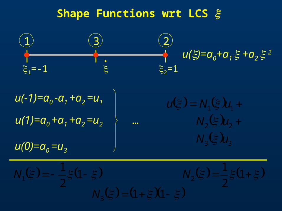
Shape Functions wrt LCS

113N

12

11N 1

2

12N

u(-1)=a0 -a1 +a2 =u1

u(1)=a0 +a1 +a2 =u2

u(0)=a0 =u3

33

22

11

uN

uN

uNu

…

u()=a0+a1 +a2 2

1=-1

1

2=1

3 2

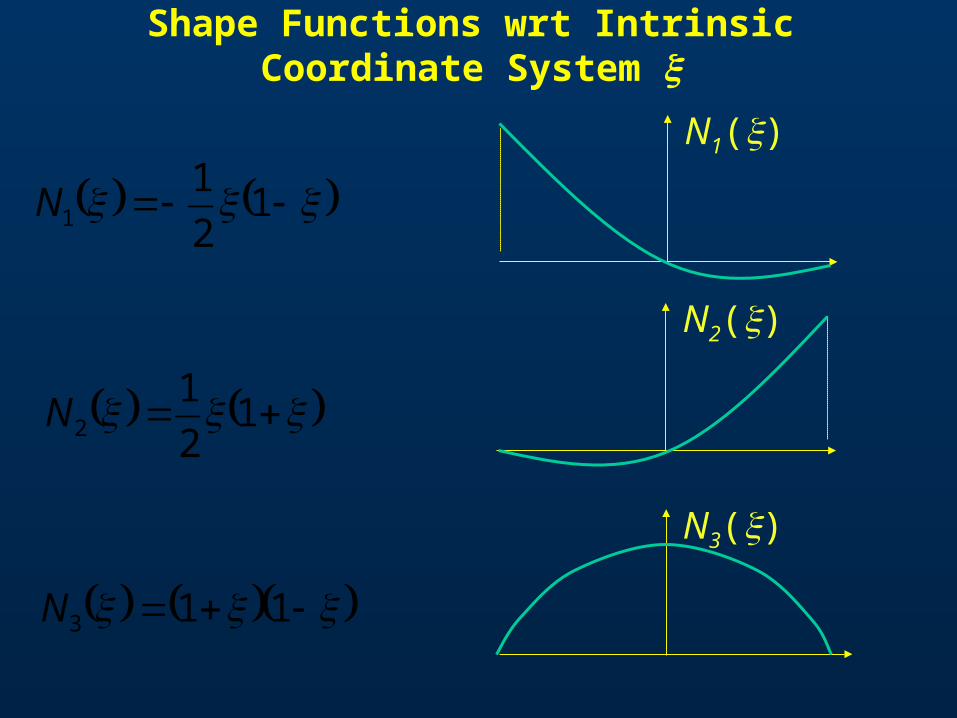
Shape Functions wrt Intrinsic Coordinate System

12

11N

N1()

12

12N

N2()

113N

N3()

wrt

dx

d

d

du

dx

xdu )()(

1

12

22

Jlxxdx

d

e

321 22

21

2

21uuu

d

du

12

11N 1

2

12N 113N

332211 uNuNuNu

Element Strain-Displacement Matrix

321 421211

uuule

3

2

1

421211

u

uu

le

Cast in Matrix Form

e= B ue

e= E B ue

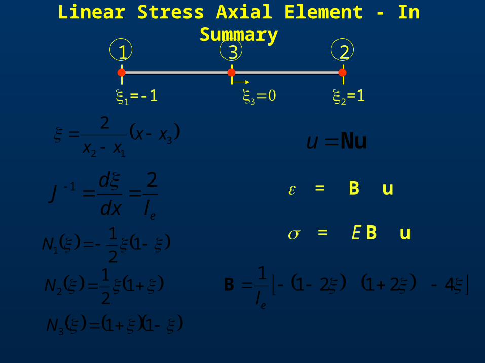
Linear Stress Axial Element - In Summary

312

2xx

xx

= B u

= E B u

Nuu

eldx

dJ

21

12

11N

12

12N

113N

421211

el

B

1=-1

1

2=1

3 2

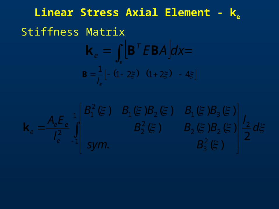
Linear Stress Axial Element - ke

1

1

2

23

2222

312121

2 2)(.

)()()(

)()()()()(

dl

Bsym

BBB

BBBBB

l

EA

e

eeek

421211

el

B

el

Te dxAEBBk

Stiffness Matrix

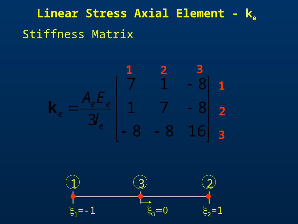
Linear Stress Axial Element - ke

1688

871

817

3 e

eee l

EAk

Stiffness Matrix

1=-1

1

2=1

3 2

1

2

3

1 2 3

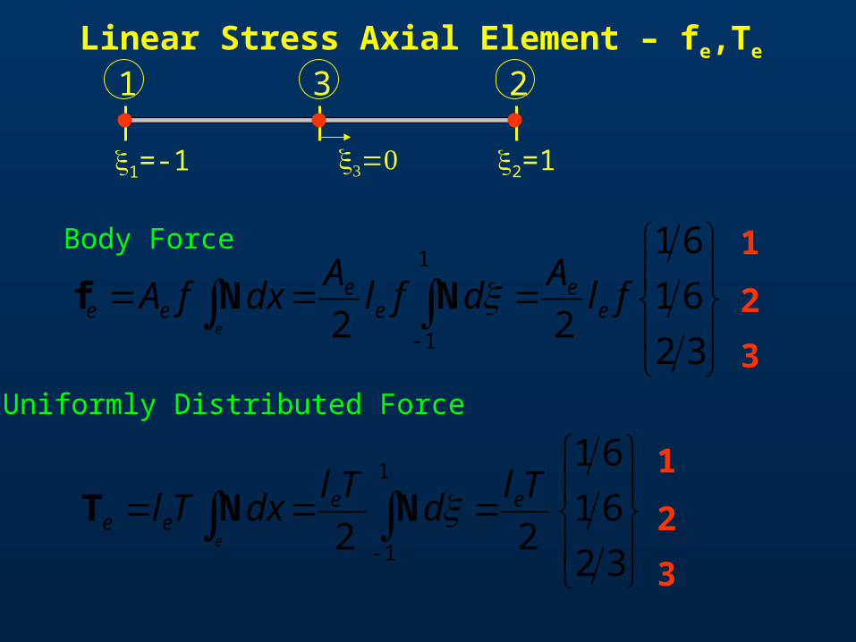
Linear Stress Axial Element – fe,Te

32

61

61

22

1

1

flA

dflA

dxfA ee

ee

leee

NNf

32

61

61

22

1

1

Tld

TldxTl ee

leee

NNT

1

2

3

1

2

3

1=-1

1

2=1

3 2

Body Force

Uniformly Distributed Force