Efficient Algorithms for Path Problemsin Weighted Graphs

Virginia Vassilevska

August 20, 2008

CMU-CS-08-147

School of Computer ScienceCarnegie Mellon University

Pittsburgh, PA 15213

Thesis Committee:Guy Blelloch, Chair

Manuel BlumAnupam Gupta

Uri Zwick (Tel Aviv University)

Submitted in partial fulfillment of the requirementsfor the degree of Doctor in Philosophy.

c©2008 Virginia Vassilevska

This research was sponsored by the National Science Foundation under contracts no. CCR-0122581, no. CCR-0313148, and no. IIS-0121641. The views and conclusions contained in this document are those of the author andshould not be interpreted as representing the official policies, either expressed or implied, of any sponsoring institution,the U.S. government or any other entity.

Keywords: shortest paths, matrix multiplication, bottleneck paths, earliest arrivals

To my parents.

1

2

Abstract

Problems related to computing optimal paths have been abundant in computer science since itsemergence as a field. Yet for a large number of such problems we still do not know whether thestate-of-the-art algorithms are the best possible. A notable example of this phenomenon is theall pairs shortest paths problem in a directed graph with real edge weights. The best algorithm(modulo small polylogarithmic improvements) for this problem runs in cubic time, a running timeknown since the 1960s (by Floyd and Warshall). Our grasp of many such fundamental algorithmicquestions is far from optimal, and the major goal of this thesis is to bring some new insights intoefficiently solving path problems in graphs.

We focus on several path problems optimizing different measures: shortest paths, maximumbottleneck paths, minimum nondecreasing paths, and various extensions. For the all-pairs versionsof these path problems we use an algebraic approach. We obtain improved algorithms using reduc-tions to fast matrix multiplication. For maximum bottleneck paths and minimum nondecreasingpaths we are the first to break the cubic barrier, obtaining truly subcubic strongly polynomial algo-rithms. We also consider a nonalgebraic, combinatorial approach, which is considered more efficientin practice compared to methods based on fast matrix multiplication. We present a combinatorialdata structure that maintains a matrix so that products with given sparse vectors can be computedefficiently. This allows us to obtain good running times for path problems in unweighted sparsegraphs.

This thesis also gives algorithms for some single source path problems. We obtain the firstlinear time algorithm for the single source minimum nondecreasing paths problem. We give someextensions to this, including an algorithm to find cheapest minimum nondecreasing paths.

Besides finding optimal paths, we consider the related problem of finding optimal cycles. Inparticular, we focus on the problem of finding in a weighted graph a triangle of maximum weightsum. We obtain the first truly subcubic algorithm for finding a maximum weight triangle in anode-weighted graph. We also present algorithms for the edge-weighted case. These algorithmsimmediately imply good algorithms for finding maximum weight k-cliques, or arbitrary maximumweight pattern subgraphs of fixed size.

3

4

Acknowledgements

This thesis can be seen as a collective effort of a large group of people. This group includes myadvisor and coauthors, my family and a large number of friends who stood by me during difficulttimes. I am grateful to all of you for your help and for believing in me.

Firstly, I am deeply grateful to my family: to my mother Tanya and my father Panayot wholistened to me (no matter whether I was bragging or complaining, laughing or crying), loved me andsupported me, and gave me an enormous amount of valuable advice half of which I followed and theother half of which I wish I followed. I am thankful to my brother Alexander, to my uncle Yordanand aunt Gergana for their support, and to my grandmother Genka who has always been therefor me. Mili mamo, tatko, Saxo, babo, vu$iqo i Geri, blagodar vi mnogo za neprestannata vipodkrepa i obiq!

Throughout my Ph.D studies I was skillfully guided by my advisor, Guy Blelloch. I am reallygrateful to him for being the perfect advisor for me, giving me wonderful advice and letting mehave freedom to work on my own things whenever I needed to! I would also like to thank the rest ofmy thesis committee, Anupam Gupta, Manuel Blum and Uri Zwick, for agreeing to see this thesisthrough and for giving me valuable advice about various extensions of my work.

I have written many papers (including the majority of the ones in this thesis) with one personwho also happens to be my partner in life, Ryan Williams. I am deeply grateful for his unconditionalsupport and amazing ability to calm me down and cheer me up. Being around him is truly a blessingand this thesis may not have been finished if it had not been for him.

During the last five years, I have had the pleasure to work with several different people on variousprojects: Raphael Yuster, Maverick Woo, Umut Acar, Srinath Sridhar, Daniel Golovin, MichelleGoodstein. Thank you for the awesome ideas and creativity! The Carnegie Mellon computer sciencefaculty has been an invaluable resource for me. In particular, I would like to mention Avrim Blum,Lenore Blum and Gary Miller who gave me a lot of useful advice. I am also grateful to Guy,Anupam, Manuel and Raphael for writing recommendations for me when I was applying for jobs.

I would like to thank all of the friends I have made here at Carnegie Mellon. Hopefully I amnot missing anyone: Liz Crawford, Shobha Venkataraman, Sue Ann Hong, Joey Gonzalez, KatrinaLigett, Noam Zeilberger, Alice Brumley, Sonia Chernova and James Hays, Mike and Kelly Crawford,our champion tennis team – Anne Yust, David Abraham, Gene Hambrick, Sam Ganzfried, MaximBichuch, Dan Wendlandt, Pan Papasaikas, Vijay Vasudevan, . . . Finally, I am really grateful toMrs. Teena Williams, Jialan Wang and Nora Tu for their love and support. You all made my lifewonderful!

5

6

Table of Contents

1 Introduction 91.1 Organization of the Thesis . . . . . . . . . . . . . . . . . . . . . . . . . . . . . . . . . 101.2 Preliminaries and Notation . . . . . . . . . . . . . . . . . . . . . . . . . . . . . . . . 11

2 Matrix Multiplication and Path Problems 132.1 A Brief History of Matrix Multiplication Algorithms . . . . . . . . . . . . . . . . . . 142.2 Generalized Matrix Product . . . . . . . . . . . . . . . . . . . . . . . . . . . . . . . . 152.3 Matrix Products and Graph Paths . . . . . . . . . . . . . . . . . . . . . . . . . . . . 15

2.3.1 Three-layered graphs . . . . . . . . . . . . . . . . . . . . . . . . . . . . . . . . 152.3.2 Paths in general graphs . . . . . . . . . . . . . . . . . . . . . . . . . . . . . . 17

2.4 Semiring Frameworks . . . . . . . . . . . . . . . . . . . . . . . . . . . . . . . . . . . . 22

3 Efficient Algorithms for Some Matrix Products 253.1 Dominance Product . . . . . . . . . . . . . . . . . . . . . . . . . . . . . . . . . . . . 253.2 (+,min)-Product . . . . . . . . . . . . . . . . . . . . . . . . . . . . . . . . . . . . . . 313.3 Generalized Dominance Product . . . . . . . . . . . . . . . . . . . . . . . . . . . . . 333.4 MaxMin Product and (min,≤r)-Product . . . . . . . . . . . . . . . . . . . . . . . . . 343.5 Distance Product . . . . . . . . . . . . . . . . . . . . . . . . . . . . . . . . . . . . . . 363.6 Parallel Algorithms . . . . . . . . . . . . . . . . . . . . . . . . . . . . . . . . . . . . . 37

4 Finding Small Subgraphs 394.1 Unweighted Subgraphs . . . . . . . . . . . . . . . . . . . . . . . . . . . . . . . . . . . 40

4.1.1 Cycles . . . . . . . . . . . . . . . . . . . . . . . . . . . . . . . . . . . . . . . . 404.1.2 k-Clique and Related Problems . . . . . . . . . . . . . . . . . . . . . . . . . . 42

4.2 Weighted Subgraphs . . . . . . . . . . . . . . . . . . . . . . . . . . . . . . . . . . . . 464.3 Maximum Triangles in Edge Weighted Graphs . . . . . . . . . . . . . . . . . . . . . 484.4 Maximum Node-Weighted Triangle in Sub-Cubic Time . . . . . . . . . . . . . . . . . 49

4.4.1 A dominance product based approach . . . . . . . . . . . . . . . . . . . . . . 494.4.2 A rectangular matrix product based approach . . . . . . . . . . . . . . . . . . 514.4.3 The Czumaj and Lingas approach and applications . . . . . . . . . . . . . . . 52

5 Bottleneck Paths 555.1 All Pairs Bottleneck Paths . . . . . . . . . . . . . . . . . . . . . . . . . . . . . . . . . 56

5.1.1 Computing explicit maximum bottleneck paths . . . . . . . . . . . . . . . . . 565.2 All Pairs Bottleneck Shortest Paths . . . . . . . . . . . . . . . . . . . . . . . . . . . . 58

5.2.1 The “Short Paths, Long Paths” method . . . . . . . . . . . . . . . . . . . . . 58

7

5.2.2 APBSP . . . . . . . . . . . . . . . . . . . . . . . . . . . . . . . . . . . . . . . 585.3 Single Source Bottleneck Paths . . . . . . . . . . . . . . . . . . . . . . . . . . . . . . 60

5.3.1 Single source-single destination bottleneck paths . . . . . . . . . . . . . . . . 615.3.2 Single source-single destination bottleneck paths in directed graphs . . . . . . 63

6 Nondecreasing Paths 676.1 All Pairs Nondecreasing Paths . . . . . . . . . . . . . . . . . . . . . . . . . . . . . . 686.2 Single Source Nondecreasing Paths . . . . . . . . . . . . . . . . . . . . . . . . . . . . 706.3 Cheapest Nondecreasing Paths . . . . . . . . . . . . . . . . . . . . . . . . . . . . . . 75

7 Combinatorial Algorithms for Path Problems in Sparse Graphs 797.1 A Combinatorial Approach for Sparse Graphs . . . . . . . . . . . . . . . . . . . . . . 797.2 On the Optimality of our Algorithms . . . . . . . . . . . . . . . . . . . . . . . . . . . 817.3 Related Work . . . . . . . . . . . . . . . . . . . . . . . . . . . . . . . . . . . . . . . . 817.4 Preliminaries and Notation . . . . . . . . . . . . . . . . . . . . . . . . . . . . . . . . 827.5 Combinatorial Matrix Products With Sparse Vectors . . . . . . . . . . . . . . . . . . 827.6 Transitive Closure . . . . . . . . . . . . . . . . . . . . . . . . . . . . . . . . . . . . . 857.7 APSP on Unweighted Undirected Graphs . . . . . . . . . . . . . . . . . . . . . . . . 86

8 Open Problems 89

8

Chapter 1

Introduction

Problems related to computing optimal paths are abundant in computer science; they have beenstudied since the emergence of computer science as a field, and are at the heart of the vast majorityof applications in the real world. Yet for many of these problems we still do not know how far ourtechniques can go, and whether the state-of-the-art algorithms are the best possible. A notableexample of this phenomenon is the shortest paths problem. For instance, for finding a shortestpath between two fixed nodes in a directed graph with nonnegative real weights on the edges, theremight exist an algorithm with running time only linear in the size of the input graph. Yet, the bestknown algorithm for the problem in a general computational model (Dijkstra’s) has a logarithmicmultiplicative overhead. Furthermore, the best algorithm for finding shortest paths between allpairs of nodes in a directed graph with real edge weights runs (modulo small polylogarithmicimprovements) in cubic time, a running time known since the 1960s (by Floyd and Warshall). Ourgrasp of many fundamental algorithmic questions is far from optimal, and the major goal of thisthesis is to find some new insights into efficiently solving different path problems in graphs.

A path in a graph is a sequence of nodes, every consecutive two linked by an edge. A pathproblem in a graph has three variants:

1. single source–single destination (also called s− t): given a graph and two nodes s and t, findan optimal path from s to t,

2. single source: given a graph and node s, for every node t find an optimal path from s to t,

3. all pairs: given a graph, for every two nodes s and t find an optimal path from s to t.

There are many measures for path optimality, depending on the problem. In the simple reach-ability problem, any path is optimal, as long as it exists. In the shortest paths problem, one isgiven a graph with real weights on the edges and a path between two nodes is optimal if it has theminimum weight sum over all paths between the nodes. An obvious application of this problemis automatically finding driving directions between physical locations. Another often used mea-sure is the minimum edge on a path – the so called bottleneck. Maximizing this measure definesthe maximum bottleneck paths problem. One application of this is finding directions between twolocations for which all tunnels have as high a clearance as possible. The problem of minimizingthe largest weight edge, on the other hand, can be applied to find the least congested route in agraph representing traffic patterns. A third measure for optimal paths is the weight of the lastedge on a path, the edge weights on which form a nondecreasing sequence. Minimizing this last

9

edge weight defines the minimum nondecreasing or earliest arrival paths problem. The primaryapplication for this problem is finding an itinerary for a trip between two physical locations thatgets you to your destination as early as possible. In theoretical computer science, these problemshave been studied alongside since the 1950s. They are also very real and applicable today. Otherapplications of path problems include robot motion planning, highway and power line engineering,network connection routing, various scheduling problems, sequence alignment in molecular biology,length-limited Huffman coding, and many many others.

In the most general setting, a path problem on an edge-weighted graph G is characterized bya function that maps the set of edges of each path to a number, so that the path problem on twonodes s and t seeks to optimize its function over all paths from s to t in G. We formalize thisfurther in Chapter 2. All of the problems we consider in this thesis are solvable in polynomial time.NP-hard path problems such as Hamiltonian path do not fall into our framework.

We consider a known algebraic approach to all-pairs path problems that links the path problemto computing a matrix product over a semiring. We extend the framework to allow slightly moregeneral algebraic structures, and outline an approach to reducing a given algebraic structure matrixproduct to matrix multiplication over a ring. We then focus on some particular path problems andobtain exciting new algorithms for them using this algebraic framework. Using algorithms for fastmatrix multiplication [28] we are the first to break the cubic barrier for maximum bottleneck pathsand minimum nondecreasing paths, obtaining truly subcubic strongly polynomial algorithms. Thisresolves two 40–year old open problems.

We also consider a nonalgebraic, combinatorial approach, which is considered more efficient inpractice compared to methods based on fast matrix multiplication. We present a combinatorialdata structure that maintains a matrix so that products with given sparse vectors can be computedefficiently. This allows us to obtain good running times for many path problems in sparse graphsby improving the running times of existing algorithms using our data structure.

This thesis also gives algorithms for some single source path problems. We obtain the firstlinear time algorithm for the single source minimum nondecreasing paths problem. We give someextensions to this, including algorithms to find shortest minimum nondecreasing paths and cheapestminimum nondecreasing paths.

Besides finding optimal paths, we consider the related problem of finding optimal cycles of agiven fixed size. In particular, we focus on the problem of finding a triangle of maximum weightsum in a weighted graph. We obtain the first truly subcubic algorithm for finding a maximumweight triangle in a node-weighted graph, resolving a 30–year old open problem. We also presentalgorithms for the edge-weighted case. These algorithms immediately imply good algorithms forfinding maximum weight k-cliques, or arbitrary maximum weight pattern subgraphs of fixed size.

1.1 Organization of the Thesis

Chapter 2 introduces the algebraic framework for matrix products and path problems. Chapter3 focuses on particular matrix products and presents efficient algorithms for them. Chapter 4considers problems related to efficiently finding cycles (e.g. triangles) and fixed size k-cliquesor other small subgraphs. Chapter 5 focuses on the maximum bottleneck paths problem andsome extensions. Chapter 6 considers the minimum nondecreasing path problem and its variants.Chapter 7 presents our nonalgebraic, combinatorial algorithms based on our efficient data structurefor matrix–sparse vector products. Chapter 8 concludes the thesis, presenting some open problems.

10

1.2 Preliminaries and Notation

All of the graphs we consider in this thesis are directed, unless stated otherwise. We use the termsnode and vertex interchangeably. For directed graphs we use the terms edge and arc interchangeably.The variables m and n refer to the number of edges and nodes in a graph, respectively. Each graph,unless stated otherwise, is considered to be weakly connected, so that m ≥ n− 1. A DAG refers toa directed acyclic graph. A clique is a complete graph, and a clique on k nodes is often referred toas a Kk.

For a positive integer k, we let [k] := 1, . . . , k. We use MT to denote the transpose of a matrixM . O(·) suppresses polylogarithmic factors, i.e. O(f(n)) = O(f(n)polylog(n)). Z and R refer tothe set of integers and reals, respectively.

Models of computation. We use the addition-comparison and word RAM models in differentparts of the thesis. We use the standard addition-comparison computational model, along withrandom access to registers in all of our algebraic algorithms for path problems. The O(log n)-wordRAM model is used partially when discussing combinatorial algorithms, though the majority of ourcombinatorial algorithms work on the pointer machine model as well. The w-word RAM model isonly used in our linear time algorithm for minimum nondecreasing paths, discussed in Chapter 6.

11

12

Chapter 2

Matrix Multiplication and PathProblems

In all branches of mathematics one can find some form of matrix multiplication. The ordinary,algebraic matrix product over a ring (such as the real numbers) is the most prevalent type ofmatrix product. The algebraic product of two n × n matrices A and B is an n × n matrix C sothat for every pair of indices i, j ∈ [n], C[i, j] is given by the dot product of row i of A and columnj of B. Computing the product of two matrices efficiently is a central problem in computationallinear algebra and scientific computing; problems such as solving linear systems, inverting a matrixor computing a matrix determinant are intimately related to computing matrix-matrix products.Moreover, matrix multiplication has surprising applications in many areas of computer science withno immediate relation to linear algebra. Valiant [93] showed that given a context free grammarand a length n string, deciding if the string can be generated by the grammar can be done inasymptotically the same time as n× n matrix multiplication. Itai and Rodeh [54] showed that onecan use fast matrix multiplication to vastly improve the complexity of clique finding. Alon, Galiland Margalit [3] showed that matrix multiplication can be used to obtain a truly subcubic runningtime for all pairs shortest paths in directed graphs with weights in −1, 0, 1. Vaidya [92] showedthat even linear programming can be sped-up by using a subcubic algorithm for matrix products.

Because of its plentiful applications, matrix multiplication is widely studied in computer sci-ence. Until 1969, it was believed that matrix multiplication requires a cubic number of steps.Strassen’s discovery of his O(n2.81) time algorithm [85] was an exciting development in the field ofalgorithms and spawned a long series of new improvements to the running time of matrix multipli-cation algorithms, culminating in the current best of O(n2.376) by Coppersmith and Winograd [28].Interestingly, there is no better lower bound known than the trivial O(n2), the time that it takesto write down the output matrix.

Besides the algebraic matrix product of two matrices one could consider matrix products usingdifferent operations instead of integer sums and products. One such example is the so calleddistance product which instead of + uses a min operation on integers and instead of · uses +on integers. This chapter introduces an algebraic framework for matrix products using differentoperations. In particular, we focus on matrix products that correspond to all pairs path problems.Such frameworks have been proposed before, e.g. the semiring framework, which we describe latein this chapter. However, the known frameworks do not encompass all path problems in this thesis.In particular, they cannot capture the product corresponding to the all pairs nondecreasing paths

13

Figure 2.1: Improving the bound on ω.

problem. Our framework is slightly more general than the semiring framework and unifies the pathproblems considered in this thesis.

We begin with an overview of the algorithmic results on algebraic matrix products which werefer to simply by matrix multiplication. This nice progress on matrix multiplication algorithmsallows us to obtain better algorithms for the rest of the products in this thesis, and it gives amotivation that other matrix products can have good algorithms.

2.1 A Brief History of Matrix Multiplication Algorithms

The study of the algorithmic complexity of (algebraic) matrix multiplication is really about deter-mining the optimal value of the exponent ω for which n×n matrix multiplication is in O(nω) time.Clearly, ω ≥ 2 and Strassen showed that ω < 2.81. The first progress on improving the upper boundon ω after Strassen’s algorithm was obtained by Pan in 1978 who showed that ω < 2.79 [71]. Biniet al. [9] decreased this bound slightly to 2.78. In 1981, Schonhage [80] made another breakthroughproving the so called asymptotic sum inequality for tensors which lead to the bound ω < 2.55.Further research [72, 78, 27] showed ω < 2.50. The laser method of Strassen [86] was the nextbig development. Strassen used it to improve the bound on ω to 2.48, and in 1990 Coppersmithand Winograd used it to achieve the current best known bound of ω < 2.376. In 2003 Cohn andUmans [25] developed a new group-theoretic framework for designing algorithms for matrix mul-tiplication. This framework led to some interesting new algorithms by Cohn et al. [24], the bestof which has the same complexity as Coppersmith and Winograd’s algorithm. The authors madesome group-theoretical conjectures which would imply that ω = 2. A more detailed survey on thehistory of matrix multiplication algorithms can be found in the book by Burgisser et al. [13], or inPan’s survey [70]. Figure 2.1 shows how the bound on ω has changed between 1969 and now.

14

2.2 Generalized Matrix Product

In many applications one needs matrix products which use different operations instead of + and ·.One example is the so called Boolean matrix product in which the matrices A and B have entriesin 0, 1 and the output matrix C is given by C[i, j] =

∨k(A[i, k]∧B[k, j]), where ∨ and ∧ are the

Boolean OR and AND operators respectively. In general, we can define a matrix product over ageneral algebraic structure as follows.

Let R be a set of elements equipped with two operations ⊕ : R × R → R and : R × R → R.Let ⊕ be commutative and associative: for all x, y, z ∈ R, x⊕y = y⊕x and (x⊕y)⊕z = x⊕(y⊕z).Then for any finite set S ⊆ R,

⊕a∈S a is well-defined – we do not have to specify the order in which

the elements are summed.Let n, d, e be positive integers. Let A be an n × d matrix with entries from R and let B be a

d × e matrix with entries from R. We define the (⊕,)- product of A and B as the n × e matrixC given by

C[i, j] =⊕k∈[d]

(A[i, k]B[k, j]),∀i ∈ [n], j ∈ [e].

Fact 1 Let T be an upper bound on the time to evaluate or ⊕ on any two elements of R. Thenthe (⊕,)-product of an n× d by a d× e matrix can be computed in O(ndeT ) time.

Examples. Table 2.1 gives some examples. Two ≤ operators are used:

1. ≤b: R ∪ −∞,∞× R ∪ −∞,∞ → 0, 1 is given by x ≤b y = 1 iff x ≤ y;

2. ≤r: R ∪ −∞,∞ × R ∪ −∞,∞ → R ∪ −∞,∞ is given by x ≤r y = y if x ≤ y and ∞otherwise.

Similar ≥ operators can also be defined.

1. ≥b: R ∪ −∞,∞× R ∪ −∞,∞ → 0, 1 is given by x ≥b y = 1 iff x ≥ y;

2. ≥r: R ∪ −∞,∞×R ∪ −∞,∞ → R ∪ −∞,∞ is given by x ≥r y = y if x ≥ y and −∞otherwise.

Many of the above matrix products have symmetric ones obtained by “inverting” the operators:(∧,∨)-product, (min,max)-product, (max,≥r)-product.

2.3 Matrix Products and Graph Paths

A path or walk in a graph is a sequence of vertices every consecutive two of which are linked by anedge. If the path does not contain any repeating nodes it is called simple. The length of a path isthe number of edges in the path. We give a connection between paths and matrix products.

2.3.1 Three-layered graphs

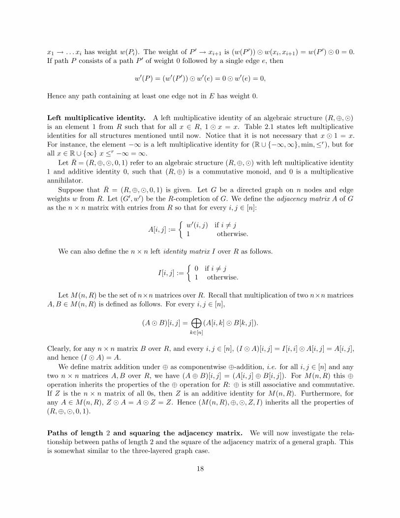
A three-layered graph G = (V,E) is a directed tripartite graph on partitions L = `1, . . . , `|L|,M = m1, . . . ,m|M | and Q = q1, . . . , q|Q|, V = L ∪M ∪ Q. The edge set E of G consists ofL×M and M ×Q. Figure 2.2 shows an example.

15

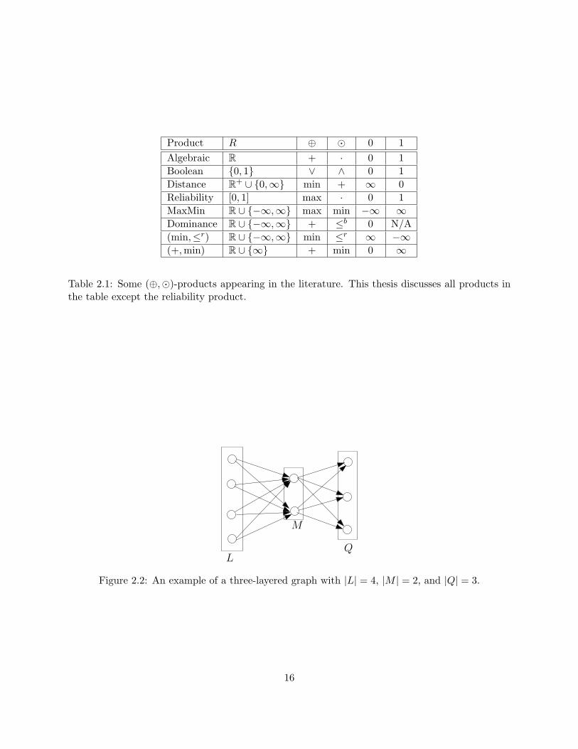
Product R ⊕ 0 1Algebraic R + · 0 1Boolean 0, 1 ∨ ∧ 0 1Distance R+ ∪ 0,∞ min + ∞ 0Reliability [0, 1] max · 0 1MaxMin R ∪ −∞,∞ max min −∞ ∞Dominance R ∪ −∞,∞ + ≤b 0 N/A(min,≤r) R ∪ −∞,∞ min ≤r ∞ −∞(+,min) R ∪ ∞ + min 0 ∞

Table 2.1: Some (⊕,)-products appearing in the literature. This thesis discusses all products inthe table except the reliability product.

L

M

Q

Figure 2.2: An example of a three-layered graph with |L| = 4, |M | = 2, and |Q| = 3.

16

Suppose that G has a weight function w : E → R defined on its edges. Let (R,⊕,) be analgebraic structure defined on R as given in the previous section. For every pair of nodes `i ∈ Land qj ∈ Q, define the length `(`i, qj) of the shortest path from `i to qj as

⊕k∈[|M |](w(`i,mk)

w(mk, qj)).Let A be an |L| × |M | matrix with entries A[i, j] = w(`i,mj). Similarly, let B be an |M | × |Q|

matrix with entries B[j, k] = w(mj , qk). Then the (i, j)th entry of the (⊕,)-product C of A andB is exactly

C[i, j] =⊕

k∈[|M |]

(w(`i,mk) w(mk, qj)) = `(`i, qj).

Hence we have shown a relationship between shortest paths in three-layered graphs with weightsfrom an algebraic structure and matrix products over the same structure.

2.3.2 Paths in general graphs

Let us now consider a general directed graph with edge weights from R. We use the followingrelatively straightforward notation using “→”: for a path P ending and node p and path Q startingat p, we denote by P → Q the path formed by first taking P and then continuing with Q; fornodes x0, x1, . . . , xk such that there is an edge (xi, xi+1) for all i = 1, . . . , k − 1, we denote byx1 → x2 → . . . → xk the path that goes through each xi consecutively, following the edges(xi, xi+1).

We define the weight of a path inductively as follows. If the path has length 0, it has weight0. If path P is just an edge (x, y), its weight w(P ) is defined to be w(x, y). If path P has lengtht > 1, i.e. P = x0 → x1 → . . .→ xt, then its weight is given by

w(P ) = (w(x0 → . . .→ xt−1)) w(xt−1, xt).

Let Pxy denote the set of all finite paths between node x and node y. We would like todefine the shortest distance between x and y as D[x, y] =

⊕P∈Pxy

w(P ). Unfortunately, as Pxy isinfinite, D[x, y] might not be well-defined. We will give some restrictive properties of (R,⊕,⊗) forwhich D[x, y] is well-defined. We note that there has been a lot of work on path algebra/semiringframeworks for path problems (see e.g. [61, 65]) that investigates a restriction of our current setting.See Section 2.4 for more details.

Additive identity and multiplicative annihilator. Suppose that there is an element 0 ∈ Rsuch that (R,⊕, 0) is an Abelian monoid: ⊕ is commutative and associative, and 0 is an identityelement, i.e. x ⊕ 0 = 0 ⊕ x = x for all x ∈ R. Moreover, suppose that 0 x = x 0 = 0 for allx ∈ R, i.e. that 0 is a multiplicative annihilator.

Given a directed graph G = (V,E) with edge weights from R, we will construct a completegraph G′ = (V, V × V ) with edge weights w′ : (V × V ) → R such that paths in G′ consisting ofedges only from E will have the same weights in G′ as in G. Paths containing at least one edgefrom (V × V ) \ E will have weight 0. This means that

⊕P from x to y w′(P ) =

⊕P from x to y w(P )

for all x, y ∈ V , and shortest distances are preserved. We call (G′, w′) the R-completion of G.This is relatively easy to accomplish. We let w′(e) = w(e) if e ∈ E and w′(e) = 0 otherwise.

Then clearly any path with edges in E will have the same weight as in G. Consider a path P withat least one edge not in E. Let (xi, xi+1) be the first edge in P that is not in E. Then P ′ = x0 →

17

x1 → . . . xi has weight w(Pi). The weight of P ′ → xi+1 is (w(P ′)) w(xi, xi+1) = w(P ′) 0 = 0.If path P consists of a path P ′ of weight 0 followed by a single edge e, then

w′(P ) = (w′(P ′)) w′(e) = 0 w′(e) = 0,

Hence any path containing at least one edge not in E has weight 0.

Left multiplicative identity. A left multiplicative identity of an algebraic structure (R,⊕,)is an element 1 from R such that for all x ∈ R, 1 x = x. Table 2.1 states left multiplicativeidentities for all structures mentioned until now. Notice that it is not necessary that x 1 = x.For instance, the element −∞ is a left multiplicative identity for (R ∪ −∞,∞,min,≤r), but forall x ∈ R ∪ ∞ x ≤r −∞ =∞.

Let R = (R,⊕,, 0, 1) refer to an algebraic structure (R,⊕,) with left multiplicative identity1 and additive identity 0, such that (R,⊕) is a commutative monoid, and 0 is a multiplicativeannihilator.

Suppose that R = (R,⊕,, 0, 1) is given. Let G be a directed graph on n nodes and edgeweights w from R. Let (G′, w′) be the R-completion of G. We define the adjacency matrix A of Gas the n× n matrix with entries from R so that for every i, j ∈ [n]:

A[i, j] :=

w′(i, j) if i 6= j1 otherwise.

We can also define the n× n left identity matrix I over R as follows.

I[i, j] :=

0 if i 6= j1 otherwise.

Let M(n, R) be the set of n×n matrices over R. Recall that multiplication of two n×n matricesA,B ∈M(n, R) is defined as follows. For every i, j ∈ [n],

(AB)[i, j] =⊕k∈[n]

(A[i, k]B[k, j]).

Clearly, for any n× n matrix B over R, and every i, j ∈ [n], (I A)[i, j] = I[i, i]A[i, j] = A[i, j],and hence (I A) = A.

We define matrix addition under ⊕ as componentwise ⊕-addition, i.e. for all i, j ∈ [n] and anytwo n × n matrices A,B over R, we have (A ⊕ B)[i, j] = (A[i, j] ⊕ B[i, j]). For M(n, R) this ⊕operation inherits the properties of the ⊕ operation for R: ⊕ is still associative and commutative.If Z is the n × n matrix of all 0s, then Z is an additive identity for M(n, R). Furthermore, forany A ∈ M(n, R), Z A = A Z = Z. Hence (M(n, R),⊕,, Z, I) inherits all the properties of(R,⊕,, 0, 1).

Paths of length 2 and squaring the adjacency matrix. We will now investigate the rela-tionship between paths of length 2 and the square of the adjacency matrix of a general graph. Thisis somewhat similar to the three-layered graph case.

18

A2[i, j] =⊕

k

(A[i, k]A[k, j]) = (2.1)

= (A[i, i]A[i, j])⊕ (A[i, j]A[j, j])⊕⊕k 6=i,j

(A[i, k]A[k, j]) = (2.2)

= (1A[i, j])⊕ (A[i, j] 1)⊕⊕k 6=i,j

(A[i, k]A[k, j]) = (2.3)

= (A[i, j]⊕ (A[i, j] 1))⊕⊕k 6=i,j

(A[i, k]A[k, j]). (2.4)

The first thing we notice is that A2[i, j] is exactly the distance between i and j if we onlyconsider paths of length 2.

Definition 2.3.1 We say that R = (R,⊕,, 0, 1) is 1-monotone if (x⊕ (x1)) = x for all x ∈ R

Using equality (2.4) we also get that if R is 1-monotone, then A2[i, j] gives the distance between iand j when only considering simple paths of length at most 2.

Right distributivity and additive idempotence. We say that R = (R,⊕,, 0, 1) is right-distributive if for all x, y, z ∈ R, (x⊕ y) z = (x z)⊕ (y z). R is idempotent if for all x ∈ R,x⊕ x = x.

Assume from now on that R has all the properties described above and is also right-distributiveand idempotent. In the standard definitions of abstract algebra, R is an idempotent non-associativenear-semiring with a left multiplicative identity, and in which 0 is both a left and a right annihilator.We will call R an algebraic path structure. Formally:

Definition 2.3.2 An algebraic path structure is an algebraic structure R = (R,⊕,, 0, 1) withthe following properties:

• (closure) for all x, y ∈ R, x⊕ y ∈ R and x y ∈ R

• (additive commutativity) for all x, y ∈ R, x⊕ y = y ⊕ x

• (additive associativity) for all x, y, z ∈ R, (x⊕ y)⊕ z = x⊕ (y ⊕ z)

• (additive identity) for all x ∈ R, x⊕ 0 = 0⊕ x = x

• (multiplicative annihilator) for all x ∈ R, x 0 = 0 x = 0

• (left multiplicative identity) for all x ∈ R, 1 x = x

• (right distributivity) for all x, y, z ∈ R, (x⊕ y) z = (x z)⊕ (y z)

• (idempotence) for all x ∈ R, x⊕ x = x

19

Let P txy be the set of paths from x to y in G of length at most t, for t ≥ 2. For t ≥ 2, define

Dt[x, y] =⊕

P∈P txy

w(P ). Then for t > 2,

Dt[x, y] =⊕

P∈P txy

w(P ) =

⊕P∈P t−1

xy

w(P )

⊕⊕

z∈V

⊕P ′∈P t−1

xz

(w(P ′) w′(z, y)

) (2.5)

=

⊕P∈P t−1

xy

w(P )

⊕⊕

z∈V

⊕P ′∈P t−1

xz

w(P ′)

w′(z, y)

(2.6)

= Dt−1[x, y]⊕⊕z∈V

(Dt−1[x, z] w′(z, y)

). (2.7)

It is tempting to define the shortest distance between two nodes x and y as D[x, y] = D[x, y]⊕(⊕

z(D[x, z]w′(z, y))), but unfortunately D[x, y] = 0 for all x, y ∈ V is a solution to this equation.We can use idempotence to obtain a better definition.

Because of our definition of the adjacency matrix, I ⊕ A = A. For t ≥ 2, let Dt be the n × nmatrix with x, y entry Dt[x, y]. Then equation 2.7 is equivalent to Dt = Dt−1 ⊕ (Dt−1 A). LetD1 = A. Then we also have D2 = A⊕ (AA) = D1 ⊕ (D1 A).

Notice that for all t ≥ 2,

Dt−1 ⊕Dt = Dt−1 ⊕Dt−1 ⊕ (Dt−1 A) = Dt−1 ⊕ (Dt−1 A) = Dt.

We show that Dt = I ⊕ (Dt−1 A) for all t ≥ 2.By induction on t. The base case is t = 2: D2 = A ⊕ (A A) = I ⊕ (I A) ⊕ (A A) =

I ⊕ (I ⊕A)A = I ⊕ (AA) = I ⊕ (D1 A).Suppose Dt−1 = I ⊕ (Dt−2 A). Since we have

Dt = Dt−1 ⊕ (Dt−1 A) = I ⊕ (Dt−2 A)⊕ (Dt−1 A) (2.8)= I ⊕ ((Dt−2 ⊕Dt−1)A) = I ⊕ (Dt−1 A). (2.9)

Now we can give a better definition which is exactly the definition used when using pathalgebras [61]:

Definition 2.3.3 The shortest distance problem for a graph with adjacency matrix A over analgebraic path structure is to find a solution (if it exists) of the equation D = I ⊕ (D A) . Werefer to such a solution as a shortest distance matrix of the graph.

If D = I ⊕ (D A) has two solutions D1 and D2, then D1 ⊕D2 is also a solution:

D1 ⊕D2 = I ⊕ I ⊕ (D1 A)⊕ (D2 A) = I ⊕ (D1 ⊕D2)A.

Then, for some algebraic path structures we can restrict the transitive closure definition as follows

Definition 2.3.4 Let R = (R,⊕,⊗, 0, 1) be an algebraic path structure for which⊕

x∈S x is well-defined for all (finite or infinite) sets S ⊆ R. Let A be a matrix over R, such that A is the adjacencymatrix of a graph G. Let ∆ ⊆M(n, R) be the set of all matrices that are solutions to the equationD = I ⊕ (D A). Then the shortest distance matrix of G with adjacency matrix A is the matrixD with

D =⊕D∈∆

D.

20

In many cases (such as for min and max), ⊕ has the property that for all x, y ∈ R, x ⊕ y ∈x, y. This defines a total order on R by x ≤ y iff x ⊕ y = x. If ∆ contains an infimum withrespect to this ordering, then the definition above can be applied even if R is not well-ordered.Under Definition 2.3.4 the shortest distance matrix is also referred to as the minimum solutionto D = I ⊕ (D A). In general, however, we will not use Definition 2.3.4. It will suffice to useDefinition 2.3.3.

Transitive closure and the path condition. The transitive closure T of a matrix A is definedas a solution of the equation T = I ⊕ (T A) in a similar way to the definition of the shortestdistance matrix (2.3.3, 2.3.4). Hence, when A is the adjacency matrix of a graph as in the previouscontext, T is also the shortest distance matrix of the graph. The transitive closure of A might notbe defined but there are many cases in which it is. Some examples can be found in Section 2.4.

Definition 2.3.5 Let R = (R,⊕,, 0, 1) be an algebraic path structure. R is said to satisfy thepath condition if for all x, y ∈ R,

x⊕ (x y) = x.

The path condition generalizes the notion of 1-monotonicity. Even though this condition seemslike a huge restriction, notice that the distance, reliability, MaxMin and (min,≤r)-products allsatisfy the path condition. These are exactly the products we will employ for path problems.

We will prove the following.

Theorem 2.3.1 Let R = (R,⊕,, 0, 1) be an algebraic path structure satisfying the path condition.Then for any graph G on R:

• the shortest distance matrix D of G is well-defined, and

• D can be computed in O(n(M(n, n)+S(n, n))) time, where M(n, n) and S(n, n) are the timeto multiply and sum (respectively) two n× n matrices over R.

Proof. Consider a path P from x to y composed of a path P1 from x to z, followed by a pathC from z back to z, followed by a path P2 from z to y. Let C = z → z1 → . . . → zp → z, andP2 = z → y1 → . . .→ yk → y. Then the weight of P is

w(P ) = (((w(P1 → C)) w(z, y1)) . . .) w(yk, y).

Consider w(P1 → P2)⊕ w(P ). This equals

(((w(P1)⊕ w(P1 → C)) w(z, y1)) . . .) w(yk, y).

From the path condition we have the following base case for our induction on j:

w(P1) = w(P1)⊕ ((w(P1)) w(z, z1)).

Assume that

w(P1) = w(P1)⊕ (((w(P1)) w(z, z1)) . . .) w(zj−1, zj).

21

Then by the path condition and the above assumption,

w(P1) = w(P1)⊕ (((w(P1)) w(z, z1)) . . .) w(zj−1, zj) (2.10)= w(P1)⊕ [(((w(P1)) w(z, z1)) . . .) w(zj−1, zj)]⊕ (2.11)⊕ [((((w(P1)) w(z, z1)) . . .) w(zj−1, zj)) w(zj , zj+1)] (2.12)= w(P1)⊕ ((((w(P1)) w(z, z1)) . . .) w(zj , zj+1). (2.13)

By the above inductive argument we obtain that

w(P1) = w(P1)⊕ w(P1 → C).

By the distributive property we also obtain that

w(P1 → P2) = w(P1 → P2)⊕ w(P1 → C → P2).

Then for any two nodes x, y, their distance can be defined as

D[x, y] =⊕

P∈Pxy

w(P ) =⊕

P∈SP x,y

w(P ),

where SP x,y is the set of all simple paths from x to y. As the number of simple paths from x to yis finite (it is at most (n− 2)!), the distance is always well-defined.

Since any simple path has length at most n, in order to compute D, it suffices to computeDn, i.e. starting from D1 = A, for i ranging from 2 to n, compute Di = I ⊕ (Di−1 A). Thiscomputation requires doing n sums and products of n× n matrices.

2.4 Semiring Frameworks

We give a brief summary of some results on path problems using the so called semiring or pathalgebra framework. Most of this can be found in the wonderful survey by Bernd Mahr [61]. Semir-ings are more restricted algebraic structures than the ones we considered in the previous section.Lengauer and Theune [60] considered converting some weaker algebraic structures into semiringsby adding the properties of associativity and distributivity. Although this approach is very general,it increases the running times of the transitive closure algorithms. From now on we only considersemirings.

A semiring or path algebra is an algebraic structure (R,⊕,, 0, 1), such that (R,⊕, 0) and(R,, 1) are both monoids, ⊕ is commutative, distributes over ⊕ (both from the right and fromthe left), and 0 is both a right and a left multiplicative annihilator. A semiring is idempotent if forall x ∈ R, x ⊕ x = x. An algebraic path structure is an idempotent semiring that is missing thefollowing properties: -associativity, left -distributivity over ⊕, and right multiplicative identity.

An idempotent semiring does not need the path condition in order to guarantee that shortestdistances are well-defined. Instead, it is sufficient if it is closed.

Closed semirings. A semiring is closed if there is a unary operation ∗ so that a∗ = 1⊕ (a a∗)for all a ∈ R. For closed idempotent semiring there is always a solution to the shortest distance

22

equation D = I ⊕ (D A). This solution is called the Kleene matrix A∗. For graphs on n nodes,A∗ = A(n), where A(0) = A, and for r > 0 and i, j ∈ [n],

A(r)ij = A

(r−1)ij ⊕

(A

(r−1)ir (A(r−1)

rr )∗ A(r−1)rj

).

The algorithms textbook by Aho, Hopcroft and Ullman [1] gives a theorem concerning thealgorithmic complexity of computing the transitive closure of a matrix over a closed semiring.Informally, this theorem, originally due to Fischer and Meyer [39], Furman [45, 46], and Munro [67],states that the transitive closure of such a matrix A can be computed in approximately the sametime as the time to multiply two matrices of the same size as A over the same semiring.

Theorem 2.4.1 ([39, 46, 67], [1], pp. 204–206) Let T (n) be the time to compute the transitiveclosure of an n× n matrix over a closed idempotent semiring R. Let M(n) be the time to computethe product of two n × n matrices over R. If M(2n) ≥ 4M(n) and T (3n) ≤ 27T (n), then T (n) =Θ(M(n)).

The theorem makes two assumptions that are very reasonable, as we expect M(n) = Ω(n2) (weneed to write the output matrix), and T (n) = O(n3) (with closed semirings we can use the Floyd-Warshall algorithm for transitive closure, see below). Furthermore, with some work these assump-tions can be weakened to M(3n) = Ω(M(n)) and T (3n) = O(T (n)).

Matrix stability. There is even a weaker condition for the transitive closure to be well-definedfor matrices over idempotent semirings. This condition is not on the semiring itself but on thegiven matrix. It requires that there is a constant q > 0, so that the matrix is q-stable.

Definition 2.4.1 A matrix A is q-stable if

q⊕r=0

Ai =q+1⊕r=0

Ai,

where A0 = I and Ai = Ai−1 A for i > 0.

The following theorem due to Floyd and Warshall [40, 99], among others, asserts that q-stabilityis a sufficient condition for the transitive closure of a matrix to be well-defined.

Theorem 2.4.2 ([40, 99]) Let R be an idempotent semiring. Let A be a q-stable square matrixover R, then A∗ =

⊕qi=0 Ai is a solution to the shortest distance equation D = I ⊕ (D A).

Theorem 2.4.2 also gives an O(n3) time algorithm for finding the transitive closure of an n× nq-stable matrix A. This algorithm is the immediate generalization of the Floyd-Warshall algorithmfor the shortest paths problem:

for all i, j = 1 to n,D[i][j] := A[i][j];

for all k, i, j = 1 to n,D[i][j] := D[i][j]⊕ (D[i][k]D[k][j]);

23

Various conditions imply the stability of a matrix. For instance, A is (n− 1)-stable if A is theadjacency matrix of a DAG, or if A is over an idempotent semiring and for all r, Ar

ii ⊕ 1 = 1. Aspecial case of this second condition is when A is the adjacency matrix of a graph G with realweights on its edges such that G has no cycles of negative weight sum. Then A is considered tobe over the so called tropical semiring (R ∪ −∞,∞,min,+,∞, 0). This ends our discussion ofsemirings. The next chapter will present good algorithms for most algebraic structure productsgiven in Table 2.1.

24

Chapter 3

Efficient Algorithms for Some MatrixProducts

In the following sections we discuss algorithms for the (⊕,⊗) matrix products defined in the previouschapter. Our algorithms are made asymptotically efficient using the subcubic results on fast matrixmultiplication [28]. We use the following general techniques.

1. Bucketting: This technique deals with preprocessing the entries of each input matrix andassigning them in a 1-to-1 fashion to some number of buckets, so that each bucket has a smallnumber of entries. After this, for each input matrix X and each bucket b, one creates a newmatrix Xb. This bucketting allows later computations to narrow the search space.

2. Bucket Processing: For each fixed bucket b, one takes the matrices Ab and Bb createdby the bucketting step and multiplies them using a different matrix product (⊕′,⊗′). Thealgorithm for this different matrix product might use these techniques recursively, or if it isjust the algebraic matrix product, fast matrix multiplication is used.

3. Exhaustive Search: The bucket processing step provides some information which allowsus to choose a small number of buckets on which the problem is solved by exhaustive search.Because the buckets are small by construction, this step takes less time than exhaustive searchon the original input.

In all of our matrix product algorithms below the above techniques are used repeatedly.

3.1 Dominance Product

We begin with the dominance product, which will be used in all of the rest of our matrix productalgorithms. Recall that this product is over the algebraic structure (R ∪ −∞,∞,+,≤b), whereon input the ordered pair (x, y), the ≤b operation returns 1 if x ≤ y and 0 otherwise.

Given a set of points v1, . . . , vn in Rd, the well-known dominating pairs problem in compu-tational geometry is to find all pairs of points (vi, vj) such that for all k = 1, . . . , d, vi[k] ≤ vj [k].This problem has many applications, for instance, in VLSI circuit design and databases.

When the number of dimensions of the space is linear in the number of points, one can computethe dominating pairs by employing the dominance product. In particular, the points are laid outas rows in a matrix A for which the columns are the coordinates. The dominance product of A

25

with its transpose At counts for each pair of points vi, vj the number of coordinates in which vj

dominates vi. Then, (vi, vj) is a dominating pair if and only if the i, j entry in AAt is exactly n.Matousek [62] gave an elegant algorithm computing the dominance product. This algorithm

uses practically the same techniques described in the beginning of this chapter.

Theorem 3.1.1 (Matousek [62]) Let A and B be real n × n matrices. The dominance productC = (AB) can be computed in O

(n

3+ω2

)time.

Proof. We outline Matousek’s approach. Consider the rows of A and columns of B together as2n points in n-dimensional space. Let the rows of A be the first n points, v1, . . . , vn, and thecolumns of B be the second n points, vn+1, . . . , v2n. For each coordinate j = 1, . . . , n, sort thepoints vi, i = 1, . . . , 2n by coordinate j. This takes O(n2 log n) time.

Define the jth rank of point vi, denoted as rj(vi), to be the position of vi in the sorted list forcoordinate j. Let s ∈ [log n, n] be a parameter to be determined later. This parameter correspondsto a bound on the size of a bucket, in our techniques. We have a bucket for each k ∈ [n/s]. Definen/s pairs of (0, 1) matrices (A1, B1), . . ., (An/s, Bn/s) as follows:

Ak[i, j] = 1 ⇐⇒ rj(vi) ∈ [ks, ks + s),

Bk[i, j] = 1 ⇐⇒ rj(vi+n) ≥ ks + s.

This concludes the bucketting step.Now, multiply Ak with BT

k , obtaining a matrix Ck for each bucket k = 1, . . . , n/s. Then Ck[i, j]equals the number of coordinates c such that vi[c] ≤ vj [c], rc(vi) ∈ [ks, ks + s), and rc(vj) ≥ ks + s.Therefore, letting

C =n/s∑k=1

Ck,

we have that C[i, j] is the number of coordinates c such that brc(vi)/sc < brc(vn+j)/sc. Thisconcludes the bucket processing step.

Suppose we compute a matrix E such that E[i, j] is the number of coordinates c such thatvi[c] ≤ vj [c] and brc(vi)/sc = brc(vn+j)/sc. Then, defining D := C + E, we will have the desireddominance product matrix

D[i, j] = |k | vi[k] ≤ vj [k]|.

To compute E, we use the n sorted lists. For each pair (i, j) ∈ [n] × [n], we look up vn+i’sposition p in the sorted list for coordinate j. By reading off the adjacent points less than vn+i inthis sorted list (i.e. the points at positions p− 1, p− 2, etc.), and stopping when we reach a pointvk such that brj(vk)/sc < brj(vn+i)/sc, we obtain the list vi1 , . . . , vi` of ` ≤ s points such thatix ∈ [n], vix [j] ≤ vn+i[j] and brj(vn+i)/sc = brj(vix)/sc. For each x = 1, . . . , `, if ix ≤ n, we add a1 to E[ix, i]. Assuming constant time lookups and constant time probes into a matrix, this entireprocess takes only O(n2s) time. This concludes the exhaustive search step.

The runtime of the above procedure is O(n2s + ns nω). Choosing s = n

ω−12 , the time bound

becomes O(n3+ω

2 ). We note that the dominance product allows us to easily obtain a subcubic algorithms for the

(+, <), (+, >) and (+,=)-products, where <,>,= on input a, b return 1 if a < b, a > b and a = brespectively, and 0 otherwise.

26

Corollary 3.1.1 If the dominance product of two arbitrary real n × n matrices can be computedin O(D(n)) time, then the (+,=), (+, <) and (+, >)-products of two arbitrary real n× n matricescan all be computed in O(D(n)) time. Hence these products are all computable in O(n

3+ω2 ).

Proof. Let A and B be the matrices for which we want to compute C,C> and C> such that forall i, j ∈ [n]

C=[i, j] =n∑

k=1

(A[i, k] = B[k, j]),

C<[i, j] =n∑

k=1

(A[i, k] < B[k, j]),

C>[i, j] =n∑

k=1

(A[i, k] > B[k, j]).

Compute the dominance product C≤ of A and B and the dominance product C≥ of B and A.For every i, j ∈ [n], let

C=[i, j] = C≤[i, j] + C≥[i, j]− n,

C<[i, j] = C≤[i, j]− C=[i, j],C>[i, j] = C≥[i, j]− C=[i, j].

There has been no progress on obtaining faster algorithms for the dominance product since

Matousek’s algorithm. Since no lower bounds for the problem are known it is still possible thatthere is an O(nω) algorithm for the dominance product of two n × n matrices. It is also possiblethat the (+,=)-product of two matrices is computationally easier than the dominance product. Wecurrently also do not know a better algorithm for the so called existence-dominance product whichhas a 1 in the i, j entry if the dominance product in that entry is n and 0 otherwise. In the followingpages we give better algorithms for the dominance product for two special cases.

The low dimensional case. Here we give a slight but useful extension of the Matousek’s algo-rithm that uses rectangular matrix multiplication to get an improved time bound, when the pointsare in Rd with d << n. This result appears in [95].

Theorem 3.1.2 Given an n×d matrix A and a d×n matrix B, the dominance matrix C of A andB can be computed in O(n1.898 ·d0.696 +n2+ε) time for all ε > 0 if d = O(n

ω−12 ), or in O(n ·d2 +nω)

time for all d.

So for example, when d = o(n0.688), we can compute the dominance matrix in o(nω).Let ω(n, d, m) denote the exponent of multiplying an n × d by a d × m matrix. We recall a

Lemma by Huang and Pan [53] also appearing in [106]:

Lemma 3.1.1 ([53]) Let α = sup0 ≤ r ≤ 1 | w(n, nr, n) = 2 + o(1) > 0.294. Then for alld ≥ nα, one can multiply an n× d by a d× n matrix in time

O(dω−21−α · n

2−ωα1−α ) = O(d0.533n1.844).

27

Proof of Theorem 3.1.2. We begin analogous to Matousek’s approach. The rows of A andcolumns of B are considered as 2n points in d-dimensional space: the rows of A are the first npoints, v1, . . . , vn, and the columns of B are the second n points, vn+1, . . . , v2n. As before,for each coordinate j = 1, . . . , d, sort the points vi, i = 1, . . . , 2n by coordinate j. This takesO(nd log n) time.

Recall, the jth rank of point vi, denoted as rj(vi), is the position of vi in the sorted list forcoordinate j. Let s ∈ [log n, n] be a parameter corresponding to a bound on the size of a bucket.Define n/s pairs of n×d (0, 1) matrices (A1, B1), . . ., (An/s, Bn/s) as follows. For k ∈ [n/s], i ∈ [n],j ∈ [d],

Ak[i, j] = 1 ⇐⇒ rj(vi) ∈ [ks, ks + s),

Bk[i, j] = 1 ⇐⇒ rj(vi+n) ≥ ks + s.

This concludes the bucketting step.The bucket processing step differs from the original Matousek approach. Instead of defining

matrices Ck, we simply compute

C =[

A1 A2 · · · An/s

]·

B1

B2...

Bn/s

,

that is, we are multiplying an n × dn/s and a dn/s × n matrix. This concludes the bucketprocessing step.

As in the Matousek approach we compute a matrix E such that E[i, j] is the number of coor-dinates c such that vi[c] ≤ vj [c] and brc(vi)/sc = brc(vj)/sc. Then, defining D := C + E, we willhave the desired dominance product matrix

D[i, j] = |k | vi[k] ≤ vj [k]|.

Computing E in this situation proceeds as before and can be verified to take O(n · d · s) time. Thisconcludes the exhaustive search step.

As before, our goal is to choose s optimally so that this runtime is minimized. Results of Huangand Pan [53] (see Lemma 3.1.1) on rectangular matrix multiplication, coupled with the optimalchoice of s show that we can either compute the dominance matrix in

O(n2ω−ωα−2

ω−α−1 · d2ω−4

ω−α−1 + n2+ε) ≤ O(n1.898d0.696)

time for all ε > 0. We can only make this choice of s when d = O(nω−1

2 ). By a slight modificationof the algorithm we can obtain an O(n · d2 + nω) runtime for all d = O(n). To do this, again sortthe columns of A and rows of B but now bucket the sorted lists into buckets of size d. Createtwo matrices A′ and B′, both n× n. The columns of A′ and rows of B′ are labeled by pairs (j, b)where j is a column of A (row of B) and b is a bucket from 1 to n/d. (There are at most n suchpairs.) A′[i, (j, b)] is 1 if A[i, j] is in bucket b of the jth sorted list, and A′[i, (j, b)] = 0 otherwise.B′[(j, b), k] is 1 if there is some b′ > b such that B[j, k] is in bucket b′ of the jth sorted list, andB′[(j, b), k] = 0 otherwise. Within buckets we do exhaustive search in overall O(nd2) time and tocount between buckets we compute A′ ·B′ over the integers in O(nω) summing the results.

28

The sparse case. In some of our applications that use a dominance product, we only want toperform comparisons with certain entries of the matrices. For example, suppose matrices A and Bare over R∪ −∞,∞, such that A has mostly ∞ entries, while B has mostly finite entries. Then,in the computation of the dominance product A B, many of the comparisons (A[i, k] ≤ B[k, j])are false; it only makes sense to compare the finite entries of A with entries in B. To this end,we design a special algorithm for dominance product in the case where one wishes to ignore largeportions of the A-matrix. The algorithm again uses the techniques described in the beginning ofthis chapter. It was published in [97].

Theorem 3.1.3 (Sparse Dominance Product) Let A and B be n×n matrices over R∪−∞,∞.Let S ⊆ [n]× [n] such that |S| = m ≥ n. Let C be the matrix such that

C[i, j] = |k | (i, k) ∈ S and A[i, k] ≤ B[k, j]|.

There is an algorithm SD that, given A, B, and S, outputs C in O(√

m · n1+ω

2 ) time.

Proof. Call the entries of A with coordinates in S the relevant entries of A. For every j = 1, . . . , n,let Lj be the sorted list containing the relevant entries from A in column j, along with the entriesfrom BT in column j. Let gj be the number of relevant entries of A in Lj , for all j. Clearly,∑

j gj = m. Pick a parameter r and partition each Lj into r consecutive buckets, such that everybucket contains at most dgj/re relevant entries of A. Note that the bucket sizes are not necessarilyuniform.

To conclude the bucketting step, for every bucket number b = 1, . . . , r, create Boolean matricesAb and Bb:

Ab[i, j] :=

1 if A[i, j] is in bucket b of Lj

0 otherwise,

Bb[j, k] :=

1 if B[j, k] is in bucket b′ of Lj and b′ > b0 otherwise.

For each bucket number b, compute Cb = Ab · Bb. This step takes O(rnω) time and computesfor every pair i, k and bucket number b, the number of j such that A[i, j] ≤ B[j, k], where A[i, j] isin bucket b of Lj , and B[j, k] is in a different bucket of Lj . This concludes the bucket processingstep.

Initialize an n × n matrix D to be all zeros. In every bucket b of Lj , there are at most dgj/rerelevant entries of A and some number tjb of entries from B. Compare every A-entry with everyBT -entry in bucket b of column j in O(tjb · dgj/re) time; in particular, for each A[i, j] ≤ BT [k, j]where A[i, j] and BT [k, j] are in bucket b, increment D[i, k]. Over all j and b, this takes time onthe order of ∑

j

∑b

tjb · dgj/re ≤∑

j

(1 + gj/r)∑

b

tjb

=∑

j

(1 + gj/r)n

= n2 +∑

j

gjn/r

= n2 + mn/r.

29

After all buckets of all lists are processed, D[i, k] contains the number of j such that A[i, j] ≤ B[j, k],where A[i, j], BT [k, j] are in the same bucket of Lj . This concludes the exhaustive search step.

Finally, set C =∑r

b=1 Cb + D. It is easy to verify from the above that the algorithm returnsthe desired C. The overall runtime of the above procedure is O(n2 + mn/r + rnω). Choosingr =√

m · n1−ω

2 , the runtime is minimized to O(√

m · n1+ω

2 ).

Corollary 3.1.2 There is an O(min(|SA| · |SB|)ω−2

ω−α−1 n(2−αω)ω−α−1 , nω +

√|SA| · |SB| ·n

ω−12 ) algorithm

for sparse dominance product, where SA and SB are subsets of [n] × [n], and the resulting matrixhas C[i, j] = |k | A[i, k] ≤ B[k, j], (i, k) ∈ SA, (k, j) ∈ SB|.

Proof. Suppose A has m1 relevant entries and B has m2. Sort each column k of A and row kof B together. For each k, let Lk be the sorted list for column/row k. Bucket each list Lk intoconsecutive buckets, so that each bucket has at most m1/D elements of A. Compare elementswithin bucket b of list k in ∑

b

gbkdm1/De

where gbk is the number of B-elements in bucket b of Lk. Overall, the runtime is O(m2 +m1m2/D).To handle comparisons between buckets we do the following (similar to our approach for rectangulardominance product). Create matrices C and C ′ where C is n × O(D) and C ′ is O(D) × n. Thecolumns of C and rows of C ′ have indices (k, b) for bucket b of Lk, provided Lk has at least 2buckets. We set C[i, (k, b)] to be 1 if A[i, k] is in bucket b of Lk. We set C ′[(k, b′), j] to be 1 ifB[k, j] is in some bucket b > b′ of Lk. Then clearly C[i, (k, b)] · C ′[(k, b), j] = 1 iff there is someb′ > b such that B[k, j] is in bucket b′ of Lk but A[i, k] is in bucket b < b′ of Lk and when we sumthese we always count different comparisons. The number of coordinates (k, b) is at most∑

k: Lk has ≥ 2 buckets

(dm1kD/me) ≤ D + D = 2D.

If D ≥ n, we can compute the product of C and C ′ in O((D/n)nω) time. For this case, the bestvalue for D is

m1m2/D = Dnω−1 =⇒ D =√

m1m2/nω−1

2

The final runtime is then O(√

m1m2nω−1

2 ).

If D = o(n), then the product of C and C ′ can be computed in O(Dω−21−α n

2−αω1−α ) time by

Lemma 3.1.1 where the current best value for α is 0.294. The best value for D is then

m2m1/D = Dω−21−α n

2−αω1−α =⇒ D =

(m1m2)1−α

ω−α−1

n(2−αω)ω−α−1

.

The final runtime becomes asymptotically

(m1m2)ω−2

ω−α−1 n(2−αω)ω−α−1 = (m1m2)0.33n1.21.

The runtime of the corollary above can be further improved for

√m1m2 = o(n

ω+12 ) using the

fast sparse matrix multiplication of Yuster and Zwick [104].One can combine Theorem 3.1.3 and the rectangular matrix multiplication from Lemma 3.1.1

to obtain a more general result.

30

Corollary 3.1.3 Let A be an n × d matrix and B be a d × n matrix over R ∪ −∞,∞. LetS ⊆ [n]× [d] such that |S| = m with n ≤ m ≤ nω/d. Let C be the matrix such that

C[i, j] = |k | (i, k) ∈ S and A[i, k] ≤ B[k, j]|.

There is an algorithm that, given A, B, and S, outputs C in O(√

md0.267n1.422) time.

Proof. The matrices Ab and Bb in the proof of Theorem 3.1.3 are now n×d and d×n respectively.Hence computing Cb = Ab ·Bb takes

O(rdw−21−α n

2−ωα1−α ) = O(rd0.533n1.844)

time by Lemma 3.1.1. The exhaustive search portion of the algorithm takes O(nd + mn/r) time.We minimize the runtime:

rdw−21−α n

2−ωα1−α = mn/r =⇒ r =

√m/(d

ω−22(1−α) n

1+α−ωα2(1−α) ).

The runtime becomesO(√

mdω−2

2(1−α) n3−α−ωα2(1−α) ) = O(

√md0.267n1.422).

3.2 (+, min)-Product

The proof approach of Theorem 3.1.1 can be extended to obtain a similar algorithm for the (+,min)-product.

Theorem 3.2.1 Given two n× n matrices A and B over R ∪ ∞, their (+,min)-product C canbe computed in O

(n

3+ω2

)time.

Proof. The proof is a slight generalization of the proof of Theorem 3.1.1. As before, consider therows of A and columns of B together as 2n points in n-dimensional space: be the first n points,v1, . . . , vn are the rows of A and the second n points, vn+1, . . . , v2n are the columns of B. Again,for each coordinate j = 1, . . . , n, sort in O(n2 log n) time vi, i = 1, . . . , 2n by coordinate j.

We will first compute C1[i, j] =∑

c: A[i,c]≤B[c,j] A[i, c], then C2[i, j] =∑

c: A[i,c]>B[c,j] B[c, j] andthen sum them in O(n2) time. We will only consider C1 in the following as computing C2 isanalogous.

Recall, rj(vi) is the position of vi in the sorted list for coordinate j. Let s ∈ [log n, n] be aparameter to be determined later, corresponding to a bound on the size of a bucket. Define then/s pairs of matrices (A1, B1), . . ., (An/s, Bn/s) as follows:

Ak[i, j] =

A[i, j] if rj(vi) ∈ [ks, ks + s),0 otherwise.

Bk[i, j] =

1 if rj(vn+i) ≥ ks + s,0 otherwise.

Notice that this is the first place where the algorithm differs from that in Theorem 3.1.1. Thisconcludes the bucketting step.

31

Now, multiply Ak with BTk , obtaining a matrix Ck for each bucket k = 1, . . . , n/s. Then

Ck[i, j] equals the sum of entries A[i, c] over coordinates c such that rc(vi) ∈ [ks, ks + s), andrc(vn+j) ≥ ks + s. In particular, for all such c we have A[i, c] ≤ B[c, j]. Therefore, letting

C ′ =n/s∑k=1

Ck,

we have that C ′[i, j] is the sum of A[i, c] over all c such that A[i, c] ≤ B[c, j], brc(vi)/sc <brc(vn+j)/sc. This concludes the bucket processing step.

Suppose we compute a matrix E such that E[i, j] is the sum of A[i, c] over all coordinates cwith A[i, c] ≤ B[c, j], and brc(vi)/sc = brc(vn+j)/sc. Then, defining C1 := C ′+E, we will have thedesired product matrix

C1[i, j] =∑

c: A[i,c]≤B[c,j]

A[i, c].

To compute E, we use the n sorted lists, as in Theorem 3.1.1. For each pair (i, j) ∈ [n]× [n], welook up vn+i’s position p in the sorted list for coordinate j. By reading off the adjacent points lessthan vn+i in this sorted list (i.e. the points at positions p− 1, p− 2, etc.), and stopping when wereach a point vk such that brj(vk)/sc < brj(vn+i)/sc, we obtain the list vi1 , . . . , vi` of ` ≤ s pointssuch that vix [j] ≤ vn+i[j] and brj(vn+i)/sc = brj(vix)/sc. For each x = 1, . . . , `, if ix ≤ n, we addA[ix, j] to E[ix, i]. Assuming constant time lookups and constant time probes into a matrix, thisentire process takes only O(n2s) time. This concludes the exhaustive search step.

The runtime of the above procedure is O(n2s + ns nω). Choosing s = n

ω−12 , the time bound

becomes O(n3+ω

2 ). Results similar to Theorems 3.1.2 and 3.1.3 are also possible for the (+,min)-product.

An application of the (+,min)-product. In the following application, we show how the domi-nance and (+,min)-products can be used to improve the runtime for solving a problem arising incomputational economics. Suppose we have a set C = 1, . . . , k of commodities, a set B of buyersand a set S of sellers. Let |C| = k, |B| = |S| = n. Each buyer bi ∈ B has a set of commoditiesCi ⊆ C. Buyer i also has a maximum price pij that i is willing to pay for item j in Ci. Each sellersi ∈ S owns a set Si ∈ C of commodities that he is willing to sell, but for each commodity j he hasa reserve price rij that needs to be met in order for the item to be exchanged.

Let us imagine that each buyer wants to do business with only one seller, and each seller wantsto target a single buyer. Each of them wish to be matched up so that they maximize the numberof transactions. Buyer i prefers seller j to seller j′, if j has more cheap items than j′ does, withrespect to the values of i. Formally, the number of commodities k for which rjk ≤ pik exceeds thenumber of commodities k for which rj′k ≤ pik.

More generally, the preferences of a buyer (or seller) may depend on more than just the numberof items that can be exchanged. These preferences may depend on both the sums of maximumprices that the buyer has for the items, and on the sums of reserves that the seller has for them.

Ideally, each buyer wants to talk to the seller from whom he can obtain the cheapest large set ofitems. Unfortunately, this is not always possible for all buyers, even when the prices and reservesare all equal. This is evidenced by the following example: Buyer 1 wants to buy item 2, buyer 2wants to buy items 1 and 2, seller 1 has item 1, seller 2 has items 1 and 2. When the preferences

32

are only according to the number of items that can be exchanged, buyer 1 will not be able to getany items.

In a realistic setting, we want to find a buyer-seller pairing so that there is no pair (b, s) forwhich buyer b is not paired with seller s, such that both b and s would benefit from breaking theirmatches and pairing among each other. This is the stable matching problem, for which optimalalgorithms are known when the preferences are known (e.g., Gale-Shapley [48] can be implementedto run in O(n2)). However, for large k, the major bottleneck in our setting is that of computingthe preference lists of the buyers and sellers.

The obvious approach gives an O(kn2) algorithm. Using the dominance product we can computea matrix C so that Cij is the number of items k for which pik ≥ rjk, i.e. the number of itemsthat can be exchanged if i and j were paired. Then the rows and columns of C can be sorted inorder to obtain a preference list for each buyer or seller. The entire procedure then would takeO(n

√kM(n, k) + n2 log n) where M(n, k) is the time required to multiply an n × k by a k × n

matrix.To do this, for each buyer i we create a k-dimensional vector bi = bi1, . . . , bik so that bij = pij if

j ∈ Ci, and bij = −∞ if j /∈ Ci. For each seller i we create a k-dimensional vector si = si1, . . . , sikso that sij = rij if j ∈ Si, and sij =∞ if j /∈ Si. Let S be the matrix with rows si and let B be thematrix with columns bi. Computing the dominance product matrix of S and B computes exactlythe number of items ` which buyer i wants to buy, seller j wants to sell, and pi` ≥ rj`.

By using the (+,min)-product instead we can actually compute, for all buyers i and seller j,both

• the sum of prices of all items that each i and j can exchange (compute and negate the(+,min)-product of (−B) with (−S)), and

• the sum of reserve prices for these exchange items (compute the (+,min)-product of S withB).

Doing this will allow us to compute any preference function on these two values, and will give a wayto solve the more general buyer-seller stable matching problem fast. In particular, the preferencelists for all buyers and sellers can be determined in O(n

√kM(n, k) + n2 log n + n2T ), where T is

the maximum time to compute the preference functions of the buyers/sellers, given the buyer priceand seller reserve sums for a buyer-seller pair. For instance, if k = n and T = O(log n), the runtimeof finding a buyer-seller stable matching is O(n

3+ω2 ) = O(n2.688).

3.3 Generalized Dominance Product

Let (⊕,) be a matrix product of n × n matrices over some algebraic structure R containingan element 0 ∈ R such that for all x ∈ R, 0 x = x 0 = 0 and x ⊕ 0 = 0 ⊕ x = x. The(⊕,)-dominance product is defined as follows.

Definition 3.3.1 Let A and B be two n × n matrices. The entries of A and B are pairs ofelements: A[i, k] = (A1[i, k], A2[i, k]) and B[i, k] = (B1[i, k], B2[i, k]) such that A1[i, k], B1[i, k] ∈ Rand A2[i, k], B2[i, k] ∈ R. The (⊕,)-dominance product matrix C is given by

C[i, j] =⊕

k∈[n],A2[i,k]≤B2[k,j]

(A1[i, k]B1[k, j]).

33

Clearly, an O(t(n)) time algorithm for the (⊕,)-dominance product of two n×n matrices canbe used to compute the (⊕,)-product of two n × n matrices in O(t(n)) time by simply addinga second component equal to 1 to all matrix entries. We show that an efficient algorithm for the(⊕,)-product can be used to obtain an efficient algorithm for the (⊕,)-dominance product.

Theorem 3.3.1 Suppose there is an O(T (n)) time algorithm for the (⊕,)-product of two n× nmatrices. Then there is an O(n1.5

√T (n)) time algorithm for the corresponding (⊕,)-dominance

product.

In particular, when T (n) = o(n3), the algorithm from the theorem is also o(n3).Proof of Theorem 3.3.1. The proof proceeds just as in Matousek’s proof of Theorem 3.1.1.Let A and B be the matrices with entries (A1[i, j], A2[i, j]) and (B1[i, j], B2[i, j]). We sort for eachk the k-th column of A and k-th row of B together in nondecreasing order of their second entrycomponents. We bucket the sorted lists Lk into buckets of size roughly s, for a parameter s to beset later. For each bucket b = 1, . . . , dn/se, create matrices Ab and Bb with

Ab[i, j] =

A1[i, j] if A[i, j] is in bucket b of Lj ,0 otherwise,

Bb[i, j] =

B1[i, j] if B[i, j] is in some bucket b′ > b of Lj ,0 otherwise.

We compute the (⊕,)-product of Ab and Bb over all b and compute the componentwise ⊕ ofall the results to obtain a matrix C. This takes O(nT (n)/s) time, provided T (n) = Ω(n2). Now, forevery entry A[i, k], let b be the bucket of Lk in which it lies. Go through all roughly s other entriesB[k, j] in that bucket and if A2[i, k] ≤ B2[k, j], add (using the ⊕ operation) (A1[i, k]B1[k, j]) toC[i, j]. This takes O(n2s) time overall provided that the ⊕ and ⊗ operations take O(1) time. Tominimize the runtime we set s =

√nT (n)/n2 and we obtain an O(n1.5

√T (n)) time algorithm for

the (⊕,)-dominance product.

3.4 MaxMin Product and (min,≤r)-Product

Recall the MaxMin product of two n×n matrices A and B over R∪−∞,∞ is defined as the matrixC such that C[i, j] = maxk minA[i, k], B[k, j] for i, j ∈ [n]. The MaxMin product is a natural gen-eralization of the Boolean matrix product to totally ordered sets of arbitrary size. In mathematics,this product is defined over the so called subtropical semiring ((R ∪ −∞,∞),max,min,−∞,∞).In computer science the MaxMin product has been studied mostly in the context of all pairs max-imum bottleneck paths (e.g. [74]), a flow problem which we will discuss in Chapter 6. Besides itsimportance in flow problems, the MaxMin product is also an important operation in fuzzy logic,where it is known as the composition of relations ([35], pp.73).

As we showed in the previous chapter, there is an easy O(n3) algorithm for the MaxMin productof two n × n matrices. Obtaining a truly subcubic algorithm (i.e. running in O(n3−δ) time forconstant δ > 0) was given as an explicit goal by Shapira, Yuster and Zwick [83]. We resolve this openproblem by showing how to reduce the MaxMin product of two n × n matrices to computing two(min,≤r)-products of n × n matrices. We then give a truly subcubic algorithm for the (min,≤r)-product of two matrices. Recall that the (min,≤r)-product of two matrices A and B over R ∪−∞,∞ is the matrix C ′ with C ′[i, j] = minB[k, j] | A[i, k] ≤ B[k, j] (C ′[i, j] = ∞ if A[i, k] >B[k, j]∀k ∈ [n]) for i, j ∈ [n].

34

Lemma 3.4.1 Suppose the (min,≤r)-product of any two n×n matrices over R∪−∞,∞ can becomputed in T (n) time. Then the MaxMin product of any two n × n matrices over R ∪ −∞,∞can be computed in O(T (n)) time.

Proof. Suppose we are given n × n matrices A and B and we wish to compute their MaxMinproduct. We create the matrices (−A) and (−B) in O(n2) time. We then compute and negate the(min,≤r)-product of (−B) and (−A) to produce a matrix A′. For every pair i, j, entry A′[i, j] givesus the maximum A[i, k] (over all k) such that A[i, k] ≤ B[k, j]. Afterwards, we compute and negatethe (min,≤r)-product of (−A) and (−B) to produce a matrix B′. For every pair i, j, entry B′[i, j]gives us the maximum B[k, j] (over all k) such that B[k, j] ≤ A[i, k]. This entire computation takesO(n2 +T (n)) time. We can assume that T (n) = Ω(n2) as one would at least have to read the input.Finally, we create a matrix C in O(n2) time with

C[i, j] = maxA′[i, j], B′[i, j], ∀i, j ∈ [n].

We now show how one can compute the (min,≤r)-product in truly sub-cubic time, reducing it

to sparse dominance with bucketting.

Theorem 3.4.1 ((min,≤r)-Product) Given two n×n matrices A and B, their (min,≤r)-productmatrix C can be computed in O(n2+ω

3 ) time. Moreover, for each pair i, j, the algorithm returns awitness k such that A[i, k] ≤ B[k, j] = C[i, j].

Proof. We begin with the bucketting phase. For every row i of matrix A, make a sorted listRi of the entries in that row. Pick a parameter g. Partition the entries of each sorted list Ri intobuckets, so that for every Ri there are dn/ge buckets with at most g entries in each bucket. Forevery bucket value b = 1, . . . , dn/ge, set up an instance (A,B, Sb) of the sparse dominance productfrom Theorem 3.1.3, where

Sb = (i, j)| A[i, j] is in bucket b of Ri.

This completes the bucketting phase. The bucket processing phase consists of actually computingthe sparse dominance product and of returning some information for the exhaustive search phase.Notice that for every bucket value b, we have |Sb| ≤ ng. By Theorem 3.1.3, all matrices Cb =SD(A,B, Sb) can be computed in

O

(n

g· √ng · n

1+ω2

)= O

(n2+ω

2

√g

).

For every pair i, j, we determine the largest bucket bi,j in Ri for which there exists a k suchthat A[i, k] ≤ B[k, j]. (This is obtained by taking the largest bi,j such that Cbi,j

[i, j] 6= 0. Note wecan easily compute bi,j during the computation of the Cb.) This concludes the bucket processingphase.

In the exhaustive search phase, for every i, j we examine the entries in bucket bi,j of Ri toobtain the maximum A[i, k] (and hence the corresponding k) such that A[i, k] ≤ B[k, j]. Sincethere are at most g entries in a bucket, each pair i, j can be processed in O(g) time. Therefore, thislast step takes O(n2g) time.

35

To pick a value for g that minimizes the runtime, we set n2g = n2+ω/2√

g , obtaining g = nω3 . The

running time is hence O(n2+ω3 ).

Plugging in the current best value for ω by Coppersmith and Winograd [28], the above timebound becomes O(n2.79). If ω = 2, then the above algorithm can run in O(n2.67). Using Lemma 3.4.1we also obtain the following corollary.

Corollary 3.4.1 The MaxMin product C of two n × n matrices A and B can be computed inO(n2+ω

3 ) = O(n2.79) time. Furthermore, for each pair i, j ∈ [n], the algorithm returns a witness ksuch that minA[i, k], B[k, j] = C[i, j].

3.5 Distance Product

Let A and B be two n × n matrices with entries in R ∪ ∞. Recall that the distance productC := A ? B is an n × n matrix with C[i, j] = mink=1...,n A[i, k] + B[k, j]. Clearly, C can becomputed in O(n3) time in the addition-comparison model, as noted in the previous chapter. Infact, Kerr [57] showed that the distance product requires Ω(n3) on a straight-line program using +and min. However, Fredman [42] showed that the distance product of two square matrices of ordern can be performed in O(n3(log log n/ log n)1/3) time. Following a sequence of improvements overFredman’s result, Chan [18] gave an O(n3(log log n)3/ log2 n) time algorithm for distance products.

Computing the distance product quickly has long been considered as the key to a truly sub-cubicAPSP algorithm, since it is known that the time complexity of APSP is no worse than that of thedistance product of two arbitrary n×n matrices. Practically all APSP algorithms with runtime ofthe form O(nα) have, at their core, some form of distance product. Therefore, any improvementon the complexity of distance product is interesting.

Seidel [82] and Galil and Margalit [50] developed O(nω) algorithms for APSP in undirectedunweighted graphs. However, for arbitrary edge weights, the best published algorithm for APSPand hence for the distance product is a recent O(n3 log log3 n/ log2 n) time algorithm by Chan [18].When the edge weights are integers in [−M,M ], the problem is solvable in O(Mnω) by Shoshanand Zwick [84], and O(M0.681n2.575) by Zwick [106], respectively. Earlier, a series of papers in the70’s and 80’s starting with Yuval [105] attempted to speed up APSP directly using fast matrixmultiplication. Unfortunately, these works require a model that allows infinite-precision operationsin constant time.

Here we show that for some nontrivial value of K, the K most significant bits of the distanceproduct A ? B can be computed in sub-cubic time, again with no exponential dependence on edgeweights. In previous work, Zwick [106] shows how to compute approximate distance products. Givenany ε > 0, his algorithm computes distances dij such that the difference of dij and the exact valueof the distance product entry is at most O(ε). The running time of his algorithm is O(W

ε ·nω log W ).

Unfortunately, guaranteeing that the distances are within ε of the right values, does not necessarilygive any of the bits of the distances. Our strategy is to use the dominance matrix product.

Proposition 3.5.1 Let A,B ∈ (Z ∪ ∞)n×n. The k most significant bits of all entries in A ? B

can be determined in O(2k · n3+ω

2 log n) time, assuming a comparison-based model.

Proof. For a matrix M , let M [i, :] be the ith row, and M [:, j] be the jth column. For a constantK, define the set of vectors

ML(K) := (M [i, 1]−K, . . . ,M [i, n]−K) | i = 1, . . . , n.

36

Also, defineMR(K) := (−M [1, i], . . . ,−M [n, i]) | i = 1, . . . , n.

Now consider the set of vectors S(K) = AL(K) ∪ BR(K). Using a dominance product compu-tation on S(K), one can obtain the matrix C(K) defined by

C(K)[i, j] :=

0 if ∃k s.t. ui[k] < vj [k], ui ∈ AL(K), vj ∈ BR(K)1 otherwise

Then for any i, j,

minkA[i, k] + B[k, j] ≥ K ⇐⇒ C(K)[i, j] = 1.

Let W be the smallest power of 2 larger than maxijA[i, j] + maxijB[i, j]. Then C(W2 ) gives

the most significant bit of each entry in A ? B. To obtain the second most significant bit, computeC(W

4 ) and C(3W4 ). The second bit of (A ? B)[i, j] is given by the expression:

(¬C(W )[i, j] ∧ C(3W4 )[i, j]) ∨ (¬C(W

2 )[i, j] ∧ C(W4 )[i, j]).

In general, to recover the first k bits of (A ? B), one computes C(·) for O(2k) values of K. Inparticular, to obtain the `-th bits, compute

2`−1−1∨s=0

[¬C(W (1− s

2`−1)) ∧ C(W (1− s

2`−1− 1

2`))].

To see this, notice that for a fixed s, if (for any i, j ∈ [n])

W (1− s

2`−1− 1

2`) ≤ min

kA[i, k] + B[k, j] < W (1− s

2`−1),

then the `-th bit of mink A[i, k] + B[k, j] must be 1, and if the `-th bit of mink A[i, k] + B[k, j] is 1,then there must exist an s with the above property.

The values for C(W (1− s2`−1 )) for even s are needed for computing the (`− 1)-st bits, hence to

compute the `-th bits, at most 2`−2 + 2`−1 dominance computations are necessary. To obtain thefirst k bits of the distance product, one needs only O(2k) dominance product computations.

3.6 Parallel Algorithms

It is well known that on an EREW-PRAM one can compute matrix multiplication with O(nω)processors in O(log n) time. We show the following.

Theorem 3.6.1 Let (⊕,) be a matrix product for which we have obtained an O(nα) algorithm inthis chapter. Then this (⊕,)-product can be computed with O(nα) processors on a EREW-PRAMin O(log n) time.

Proof. Each of our algorithms followed three steps:

37

1. Bucketting: The preprocessing step in this chapter sorts O(n2) elements and then creates Bpairs of new matrices for some value B. The sorting step can be done on an EREW-PRAMusing Cole’s mergesort algorithm with O(n2) processors and O(log n) time. Each pair ofmatrices creates a new problem instance so we have Bn2 processors, each holding an entry ofan instance.

2. Bucket Processing: For each fixed bucket instance b ∈ [B], one takes the matrices Ab

and Bb created by the bucketting step and multiplies them using a different matrix product(⊕′,⊗′). We assume that this product can be computed using O(nβ) processors and O(log n)time for some appropriate β (β = ω for Boolean matrix multiplication). Hence we haveO(Bnβ) processors solving this step in O(log n) time.

3. Exhaustive Search: We can add a processor computing each step of the exhaustive searchin parallel. Each exhaustive search step in our algorithms is an element comparison which isindependent from the other comparisons, and hence this can be done. After the comparisons,the best result from all comparisons is returned. This can be accomplished in O(log n) timeand O(n3/B) processors by a binary search approach: add processors comparing disjoint pairsof results, then processors comparing disjoint pairs of the next results and so on; the numberof new processors halves at each step and we get an asymptotic number of n3/B (this is likea binary tree circuit).

The final number of processors is minimized when B = n3−β

2 and the number of processors isO(n

3+β2 ), which is the sequential running time that we would obtain for the (⊕,)-product using

these techniques.

38

Chapter 4

Finding Small Subgraphs

Finding cliques or other types of subgraphs in a larger graph is a classical problem in complexitytheory and algorithmic combinatorics. Finding large cliques has many applications, for instance incomputational biology, classification theory, coding theory, computer vision, economics, informationretrieval, signal transmission theory etc. For detailed example applications, see [14].

Finding a maximum clique is NP-Hard, and also hard to approximate [51]. This problem is alsoconjectured to be not fixed parameter tractable [33]. The problem of finding (induced) subgraphs onk vertices in an n-vertex graph has been studied extensively (see, e.g., [4, 5, 22, 37, 58, 68, 73, 103]).All known algorithms for finding an induced subgraph on k vertices have running time nΘ(k). Manyof these algorithms use fast matrix multiplication to obtain improved exponents.

In this chapter (as in the rest of the thesis) we only consider polynomial time solvable problems.We give efficient algorithms for instances of the following general problem:

Definition 4.0.1 Let H be a fixed graph of constant size k. The H-subgraph problem on instanceG is defined as follows: Given an input graph G, find a subgraph H ′ of G isomorphic to H.

If H ′ is to be an induced subgraph of G, we refer to the problem as the induced H-subgraphproblem. If G has real weights on its vertices or edges, we further require that H ′ is an inducedsubgraph of G of maximum weight sum over all such induced subgraphs of G isomorphic to H. Theproblem is then called the maximum H-subgraph problem.

We note that finding a maximum k-clique is at least as hard as finding a maximum inducedH-subgraph, but the opposite is not necessarily true, as we show in the section on finding k-cliques.

Lemma 4.0.1 Suppose one can find a maximum weight k-clique in an n node graph in O(T (n))time. Then, for any fixed graph H on k nodes, one can find a maximum induced H-subgraph of ann node graph in O(n2 + T (n)) expected time.

Proof. Let G = (V,E) be the given graph. Let G have weights wV : V → R and wE : E → R.Create k sets S1, . . . , Sk initially empty. For every node v of the input graph G, with probabilitypi = 1/k place v in Si. In expectation, we add each node to 1 set Si. We will create a graph G′

based on G and H. G′ will have O(n) nodes in expectation.We will first define the edges of G′. Let H = (VH , EH) have nodes h1, . . . , hk. Consider every

pair of indices i, j ∈ [k], i 6= j. For every two nodes u ∈ Si, v ∈ Sj , place an edge between u and vin G′ if (hi, hj) ∈ EH and (u, v) ∈ E, or if (hi, hj) /∈ EH , (u, v) /∈ E and u 6= v. This transformation

39

takes expected O(n2) time as k is fixed and for every node of G there are only a constant numberexpected copies in G′.

Consider a subgraph H ′ = (VH′ , EH′) of G isomorphic to H so that the isomorphism maps nodeh′i of H ′ to node hi of H. Then with probability at least 1/kk for every i = 1, . . . , k, node h′i ofH ′ is in set Si. Furthermore, the nodes corresponding to the h′i in G′ form a clique as for everyi, j ∈ [k], i 6= j, (h′i, h

′j) ∈ EH′ if and only if (hi, hj) ∈ EH as H and H ′ are isomorphic.

Now suppose that a subgraph H ′ of G′ is a clique. Since no two nodes in the same set Si arelinked by an edge, the nodes h′1, . . . , h

′k are in different sets Si. Suppose for i = 1, . . . , k, node

h′i ∈ Si. As H ′ is a clique, it must be the case that all h′i correspond to distinct nodes of G.Furthermore, because of the construction of G′, since (h′i, h

′j) is an edge in G′, then (h′i, h

′j) is an

edge in G if and only if (hi, hj) is an edge in H. Thus H and H ′ must be isomorphic and H ′ is aninduced H-subgraph in G.

We now define the weights of G′. We let every node u of G′ inherit its weight wV (u) from G.If (u, v) is an edge in G′ with u ∈ Si and v ∈ Sj such that (hi, hj) ∈ EH , then let (u, v) inherit itsweight wE(u, v) from G. Otherwise, set its weight to 0. In this way, k-cliques of G′ have the sameweight sum as their corresponding H-subgraphs in G.

4.1 Unweighted Subgraphs

We first investigate the H-subgraph problem in the unweighted setting.

4.1.1 Cycles

We consider the H-subgraph problem when H is Ck, a cycle on k nodes. We give some reductionsbetween the directed and undirected versions of the problem obtaining Figure 4.1.1.

A major result on the Ck-subgraph problem was proven by Yuster and Zwick who showed thatan undirected even cycle in an n node graph can be found in O(n2) time:

Theorem 4.1.1 (Yuster and Zwick [102]) Let k > 1 be a constant. Given an undirected graphG on n nodes, a (not necessarily induced) cycle subgraph C2k on 2k nodes, if it exists, can be foundin O(n2) time.

Interestingly, for fixed k, the best known runtime bound for finding an odd Ck in an undirectedgraph, or an even directed Ck in a directed graph is O(nω). Hence the problems of finding evendirected cycles, and finding odd undirected cycles seem more difficult than the problem of findingan even undirected cycle. Our reductions in this section give some intuition about why this mightbe the case.

We will denote an undirected cycle on k nodes by Ck and a directed cycle on k nodes by−→Ck.

We first show that finding a directed k-cycle is at least as hard as finding an undirected k-cycle. Wethen show that finding an odd undirected k-cycle is at least as hard as finding a directed k-cycle.Finally we note that finding a k-cycle is at least as hard as finding a k − 1-cycle. Our results areshown pictorially in Figure 4.1.1.

Theorem 4.1.2 Let k be fixed. Suppose that there is an algorithm which given a directed n nodegraph G finds a

−→Ck subgraph of G (if it exists) in O(T (n)) time. Then there is an O(n2 + T (n))

expected time algorithm which given an undirected n node graph G′, finds a Ck subgraph of G′, ifit exists.

40

−→C4

−→C3

C3

−→C2k

−−−→C2k−1

−→C5

C5 C2k−1 C2k+1

. . .

. . .

−−−→C2k+1

. . .

. . .

Figure 4.1: An arrow from cycle C of length k to cycle C ′ means that there is an expected O(f(k)n2)time reduction from the C-subgraph problem on n node graphs to the C ′-subgraph problem onO(n) node graphs for some computable function f . Theorem 4.1.2 proves Ck → ~Ck. Theorem 4.1.3proves ~C2k+1 → C2k+1. Theorem 4.1.4 proves ~Ck → ~Ck+1. The arrows are composable, and wealso obtain C2k−1 → C2k+1.

Proof. Given an undirected graph G′ on n nodes in which we want to find a Ck, we will constructin expected O(n2) time an O(n) node graph G such that finding a

−→Ck in G corresponds to finding

a Ck in G′.Suppose we have k colors labeled 1, . . . , k. Then, for every node v of G′, color v with color i

with probability 1/k. If a node does not get any colors, flip its coins again. We expect that afterO(1) coin flips per node each node will have at least one color, and an expected O(1) colors.

For every node v of G′ and color i with which v is colored, create a node vi in G. For eachi = 1, . . . , k, create a directed edge (ui, vi+1) in G, if (u, v) is an edge of G′ and u is colored i andv is colored i + 1. Here the indices are taken mod 2k.

Any directed k-cycle of G, v11 → v2

2 → . . . → vkk → v1

1 corresponds to an undirected k-cycle ofG′, v1 → v2 → . . .→ vk → v1.

Suppose v1 → v2 → . . .→ vk → v1 is an undirected k-cycle of G′. Then with probability 1/kk,for each i = 1, . . . , k, vi received color i. Hence with probability 1/kk, v1

1 → v22 → . . . → vk

k → v11

is a directed cycle in G′. In expectation we need to repeat this reduction kk = O(1) times in orderfor the directed cycle to appear in G′.

If we consider only odd cycles, the converse of Theorem 4.1.2 also holds:

Theorem 4.1.3 Let k > 0 be fixed. Suppose that there is an algorithm that given an undirectedn node graph G finds a C2k+1 subgraph of G (if it exists) in O(T (n)) time. Then there is anO(n2 + T (n)) time algorithm that given a directed n node graph G′, finds a

−−−→C2k+1 subgraph of G′,

if it exists.

Proof. We proceed very similarly to Theorem 4.1.2. Given a directed graph G′ on n nodes inwhich we want to find a

−−−→C2k+1, we will construct in expected O(n2) time an O(n) node graph G

such that finding a C2k+1 in G corresponds to finding a−−−→C2k+1 in G′.

Suppose we have 2k + 1 colors labeled 1, . . . , (2k + 1). Then, for every node v of G′, color vwith color i with probability 1/(2k + 1). If a node does not get any colors, flip its coins again. Weexpect that after O(1) coin flips per node each node will have at least one color, and an expectedO(1) colors.

For every node v of G′ and color i with which v is colored, create a node vi in G. For eachi = 1, . . . , (2k + 1), create an undirected edge (ui, vi+1) in G, if (u, v) is a directed edge of G′ andu is colored i and v is colored i + 1. Here the indices are taken mod (2k + 1).

41

First consider a (2k + 1)-cycle of G′, say v1 → v2 → . . . → v2k+1 → v1. With probability1/(2k + 1)2k+1 this cycle appears in G as the (2k + 1)-cycle v1

1 → v21 → . . .→ v2k+1

2k+1 → v11.

Now, consider any (2k + 1)-cycle C of G. Suppose that there is some i ∈ [2k + 1] such thatC does not contain any edge (ui, vi+1 mod (2k+1)). Then C must be even. Hence the only possibleundirected (2k + 1)-cycles in G are of the form v1

1 → v21 → . . .→ v2k+1

2k+1 → v11, and they correspond

to directed cycles v1 → v2 → . . .→ v2k+1 → v1 of G′.We expect to repeat the reduction (2k)2k = O(1) times for a (2k + 1) cycle to appear in G if a

−−−→C2k+1 in G′ exists. The reduction itself takes O(n2) time.

Finally, we show that as k grows the time complexity of finding a Ck and a−→Ck grows.

Theorem 4.1.4 Let k > 2 be fixed. Suppose that there is an algorithm that given a directed n nodegraph G finds a Ck+1 subgraph of G (if it exists) in O(T (n)) time. Then there is an O(n2 + T (n))time algorithm which given a directed n node graph G′, finds a

−→Ck subgraph of G′, if it exists.

Proof. We proceed very similarly to Theorems 4.1.3 and 4.1.2. Given a directed graph G′ on n

nodes in which we want to find a−→Ck, we will construct in expected O(n2) time an O(n) node graph

G such that finding a Ck+1 in G corresponds to finding a−→Ck in G′.

Suppose we have k colors labeled 1, . . . , k. Then, for every node v of G′, color v with color iwith probability 1/(k). If a node does not get any colors, flip its coins again. We expect that afterO(1) coin flips per node each node will have at least one color, and an expected O(1) colors.

For every node v of G′ and color i with which v is colored, create a node vi in G. For eachi = 1, . . . , k − 1, create an undirected edge (ui, vi+1) in G, if (u, v) is a directed edge of G′ and uis colored i and v is colored i + 1. Here the indices are not taken mod k, so that we do not haveedges (uk, v1).

For every node v1 of G, add a new node v′1 to G and an edge (v′1, v1). For every two nodes uk

and v′1 of G such that (u, v) is a directed edge of G′, add an edge (uk, v′1) to G.

Clearly, any directed (k+1)-cycle of G has the form v11 → v2

2 → . . .→ vkk → v′11 → v1

1 and hencecorresponds to a k-cycle v1 → v2 → . . .→ vk → v1 of G′.

Conversely, a k-cycle of G′ appears in G with probability 1/kk. Hence we expect that afterO(1) repetitions of this reduction that if G′ has a k-cycle, then G will contain a (k + 1)-cycle. Thereduction takes expected O(n2) time.

It is likely that our above two results can be derandomized, perhaps using perfect hash families,as in [4]. The dependence on k in our algorithms can also probably be improved.

4.1.2 k-Clique and Related Problems

The k-clique problem is one of the fundamental problems in computer science. It is one of Karp’soriginal NP-complete problems [56]. In parametrized complexity k-clique plays a central role: oneof the major problems in this area is to resolve whether W [1] = FPT , and k-clique is W [1]-complete [34]. Furthermore, results by Chen et al. [20] imply that if there is an no(k) algorithm fork-clique 1, then many of the classical NP-complete problems are solvable in subexponential time.

The naive algorithm for k-clique runs in O(nk) time by examining all k-tuples of vertices. In1978, Itai and Rodeh [54] showed that a 3-clique (triangle) in an n-node graph can be found in thesame time as n×n Boolean matrix multiplication. Nowadays this means that there is an O(n2.376)

1here k is assumed to be any unbounded function of n

42

algorithm [28] for 3-clique; we denote this exponent by ω. In 1984 ([64], p. 46), Laszlo Lovasz askedif there is an O(n0.01k) algorithm for general k-clique. He noted that Fan Chung and Richard Karphad used Strassen’s fast matrix multiplication [85] to obtain better algorithms for 100-clique. Inthe next year, Nesetril and Poljak [69] showed how to generalize Itai and Rodeh’s [54] reduction toobtain an O(nωk) time algorithm for 3k-clique. Since that result very little progress has been made.In 2004 Eisenbrand and Grandoni [37] used rectangular matrix multiplication to obtain improvedrunning times for some values of k, e.g. for k ≥ 5 such that k = 2 mod 3.

Although these algebraic matrix product approaches yield good theoretical time bounds, theknown fast matrix multiplication algorithms that run in O(n3−ε) time for ε > 0 ([85, 28]) are veryinefficient in practice. Another issue is that all of the above mentioned algorithms for k-clique usenΩ(k) space. In fact, in the same 1984 article ([64], p.46), Laszlo Babai asked if there exists an o(nk)algorithm for k-clique using O(nc) space for some constant c independent of k. This question hasuntil now remained unanswered. In fact, the problem of designing better time and space efficientk-clique algorithms has been recently reraised by Woeginger [101].

Combinatorial, nonalgebraic algorithms based on preprocessing and table look-up offer lessimpressive asymptotic improvements but seem to be much more practical than algorithms basedon algebraic fast matrix multiplication (see Chapter 7 for combinatorial algorithms in sparse graphs).Using a “Four Russians” type approach for combinatorial matrix multiplication [6, 79, 7, 17] onecan obtain an O(nk/(k log2 n)) time algorithm for k-clique that hides no enormous constant factorsin its runtime. Nevertheless, even this algorithm is space-inefficient – it requires Ω(n2k/3) space.

In this section we answer Babai’s question in the affirmative. We give a combinatorial algorithmfor k-clique that runs in O(nk/ logk−1 n) time for every fixed k ≥ 3 and uses O(knε) space, for anyconstant ε > 0 independent of k. This algorithm is not only space-efficient but also: (a) it beatsthe runtimes of the current best combinatorial algorithms for finding k-clique for k > 3, and (b) itcan be adapted easily to obtain an algorithm for maximum node-weighted k-clique with identicalruntime. (We will give an algebraic algorithm for the node-weighted k-clique problem in the nextsection. Also note that Czumaj and Lingas [30] have shown that maximum weighted 3k-clique canbe found in O(nωk+ε) for all ε > 0 but we cannot apply their method here because of the extraO(nε) factor.)

In the second part of the section we consider finding k-node subgraphs that are almost cliques:induced subgraphs that are cliques missing one edge. This scenario is a generalization of the well-studied recognition problem for P3-free or diamond-free graphs. A folklore result shows that aninduced P3 in a graph can be found in O(n2) time. Kloks, Kratsch and Muller [58] show that aninduced diamond in a graph can be found in O(nω +m3/2) time and Eisenbrand and Grandoni [37]improve this running time to O(m3/2) by a combinatorial algorithm. We generalize these results toshow that a Kk − e in a graph can be found (if it exists) combinatorially in O(m(k−1)/2) time andO(m+n) space. This running time is better than any known combinatorial algorithm for k-clique.

Algorithm for k-Clique. We begin with a small-space combinatorial algorithm which given anode-weighted graph finds a k-clique of maximum weight sum. The basic idea used in the algorithmis to reduce the problem to finding maximum node-weighted (k−1)-cliques in many small O(log n)size subgraphs, and then attempt to complete these cliques by adding an extra node. To use smallspace, our algorithm proceeds in iterations so that each new iteration reuses the space used by theprevious ones.

Theorem 4.1.5 Let ε > 0 and k ≥ 3. Let g(k) = (2(k − 1))k−1. Let G = (V,E) be a given graph.

43

There is an algorithm for k-clique that runs in O(g(k) · nk

(ε log n)k−1

)time and uses O(knε) space.

Proof. Let G = (V,E), ε > 0 and k be given. Let ε′ = ε/(2(k − 1)).Partition the nodes into n/(ε′ log n) parts of ε′ log n nodes each. The partition is chosen by

grouping consecutive nodes according to the order of the columns in the adjacency matrix. Thisensures that any k chunks of a row corresponding to k of the (ε′ log n)-size parts can be concatenatedin O(k) time, assuming constant time look-ups and an O(log n)-word RAM.2

We will process all (k − 1)-tuples of parts as follows. Fix a (k − 1)-tuple of parts. Obtainthe union U of these parts, and create a look-up table TU with (ε′(k − 1) log n)-bit keys. For all2ε′(k−1) log n subsets of U determine whether the corresponding induced subgraph of G containsa (k − 1) clique. Store the result for each subset (a k-clique, if found) in TU , with the binary(ε′(k − 1) log n)-length vector representing the subset as the key. When a new union is processed,the look-up table information is overwritten.

Now, for every node v ∈ V , concatenate the portions of the neighborhood vector for v corre-sponding to U in O(k) time to obtain a (ε′(k − 1) log n)-bit key. Look up in TU using this keywhether the induced neighborhood of v in U contains a (k−1)-clique. If this is so, return the unionof the clique and v.Creating all tables TU takes

O((n/(ε′ log n))k−1 · nε′(k−1) · (ε′(k − 1) log n)k−1) = O(n(1+ε′)(k−1) · (k − 1)k−1)

time, and O(k log n2ε′(k−1) log n) space over all. The entire procedure (assuming O(1) time look-upsin TU ) takes O(n · (n/(ε′ log n))k−1)) time, i.e.

O(n(1+ε′)(k−1) · (k − 1)k−1 + nk/(ε′ log n)k−1)

time overall. Since we set ε′ = ε/(2(k− 1)), the runtime becomes O((2(k− 1))k−1 ·nk/(ε log n)k−1).The space usage becomes asymptotically

k log n2ε′(k−1) log n = knε/2 log n = O(knε).

One can modify the algorithm so that a maximum weight clique can be found: for every

(ε′(k − 1) log n)-node subgraph of a union of (k − 1)-tuples of node partitions, compute the themaximum weight (k − 1) clique and store that clique in the look-up table for the union. Sincethe algorithm goes over all possible choices for a k-th node, the maximum weight clique can bereturned.

Corollary 4.1.1 Let ε > 0 and k ≥ 3. Let g(k) = (2(k − 1))k−1. Let G = (V,E) be a graph witharbitrary real weights on its nodes. There is an algorithm for maximum node-weighted k-clique thatruns in O

(g(k) · nk

(ε log n)k−1

)time and uses O(knε) space.

We can use the algorithm of Theorem 4.1.5 to obtain an algorithm with a running time depend-ing on the number of edges in the graph. We use an idea used in many other results (e.g. [5]) –either the clique has all high degree vertices, or it has a low degree vertex. In both cases we canreduce the problem to finding a clique in a strictly smaller subgraph.

2The same can be accomplished on a pointer machine using some tricks.

44

Theorem 4.1.6 Let k ≥ 5 and ε > 0. Let g(k) = (2(k−1))k−1. There is an algorithm for k-clique

that runs in O(kmε/2) space and O

(g(k) · m

k2

(ε log m)(k−2− 1

k−1)

)time on graphs with m edges.

Proof. Let D be a parameter. Consider the set S of all nodes of degree at least D. There areat most m/D such nodes. Use the algorithm of Theorem 4.1.5 to find a k-clique contained in S ifone exists in O(g(k)(m/D)k/(ε log(m/D))k−1) time. If no k-clique is found in S, any k-clique inthe graph must contain a node of degree < D. Go through all edges (u, v) incident on low degreenodes, and look for a (k−2)-clique in the intersection of the neighborhoods of u and v, again usingTheorem 4.1.5. This takes time O(mg(k − 2)Dk−2/(ε log D)k−3).

To minimize the final running time of the clique algorithm, we set

mDk−2/(ε log D)k−3 = Θ((m/D)k/(ε log(m/D))k−1),

and hence D =√

m/(ε log m)1

k−1 suffices. When we plug back in, the running time becomesO(g(k)mk/2/(ε log m)(k−2− 1

k−1)). The space usage is O(k(m/D)ε) in the first part of the procedure,

and O((k− 2)Dε) in the second part. The space usage in the first part dominates and is O(kmε/2).

Finding an induced Kk−e. In graph theory, we use Kk−e to denote a k-clique missing one edge.A K3− e is also called a P3 (a path on 3 nodes), and a K4− e is a diamond. Diamond-free graphs,graphs containing no induced K4 − e, are well studied in graph theory, in particular in connectionto the strong perfect graph theorem [23] which was shown by Tucker [91] to hold for these graphs.In terms of the computational complexity of recognizing diamond-free graphs, Kloks et al. [58]showed that an induced diamond in a graph can be found in O(nω + m3/2) time. Eisenbrand andGrandoni [37] improved this running time to O(m3/2) combinatorially. We generalize this result byshowing that finding an induced Kk − e in a given graph, or recognizing (Kk − e)-free graphs canbe done combinatorially in O(m(k−1)/2) time and O(m + n) space on graphs with m edges. Ourproofs are really short and simple. We include this result to show that removing even just one edgefrom a k-clique seems to make finding an induced subgraph easier: our algorithm is faster than anyknown combinatorial algorithm for k-clique.

We begin by a lemma that gives a linear time algorithm for finding a P3. To our knowledge, theprevious best algorithm had a running time of O(n2). The following lemma also gives an example ofa case for which finding a k-clique seems harder than finding a not necessarily induced H-subgraphon k nodes. Recall that in the beginning of the chapter we showed that finding a k-clique is at leastas hard as finding an H-subgraph on k nodes.

Lemma 4.1.1 One can find an induced P3 or determine that the graph is P3-free in O(m + n)time.

Proof. We will label nodes by their first processed neighbor. Give an ordering to the nodes. Beginwith node 1. When processing node i, if i has not been labeled yet, label it i and go through all itsneighbors. Label all unlabeled neighbors i. If some neighbor x is labeled j, then j, x, i form a P3.

Suppose node i is already labeled with j. Then, if deg(i) 6= deg(j), find a node x that is in thedifference of their neighborhoods and return x, i and j as a P3. Otherwise, suppose deg(i) = deg(j).Check whether all the neighbors of i are labeled j. If so, move on to node i+1. On the other hand,if some neighbor x of i is labeled with j′ 6= j, then

45

• if j′ > j, then when j′ was processed, there was no edge between x and j and hence j, i, xform a P3;

• if j > j′, then when j was processed, there was no edge between i and j′ and hence i, x, j′

form a P3.

If some neighbor x does not have a label, then x does not have an edge to j and hence j, i, x form aP3. If by the end of the procedure no P3 was returned, then the graph is a disjoint union of cliquesand hence contains no induced P3. This is because every node i has the same neighbors as its firstencountered neighbor. This entire labeling procedure takes O(m + n) time.

Because finding induced P3 and K4−e can be done efficiently, we can give an inductive procedureto find induced Kk − e for general k ≥ 3.

Theorem 4.1.7 An induced Kk − e in a graph with m edges can be found in O(m(k−1)/2) time,for any k ≥ 3.

Proof. If k = 3, then use the algorithm from Lemma 4.1.1 to find a K3− e in O(m) time. If k = 4,use Eisenbrand and Grandoni’s algorithm to find a K4 − e in O(m3/2) time. In both cases this isO(m(k−1)/2).

Suppose k > 4. Let i = k mod 2, i ∈ 0, 1. Consider all (k − 4 + i)-cliques in the graph.There are at most m(k−4+i)/2 such cliques as each such clique can be represented as a (k− 4+ i)/2-matching. For each (k− 4 + i)-clique, in O(km) time find the intersection N of the neighborhoodsof the nodes in the clique. Then, in O(m(3−i)/2) time find an induced K4−i − e in N , or determinethat it does not exist. (Note, K4−i − e is either K3 − e or K4 − e.) The overall running timebecomes O(km(k−2+i)/2 + m(k−4+i+3−i)/2) = O(km(k−1)/2). When k is even, the running time isO(m(k−1)/2).

The algorithm from Theorem 4.1.7 runs in linear space because both Eisenbrand and Grandoni’salgorithm for finding diamonds and our algorithm from Lemma 4.1.1 use linear space, and each ofthe separate recursive calls to these algorithms are on smaller graphs.

4.2 Weighted Subgraphs

In this section we present algorithms for solving the maximum (induced) H-subgraph problem ina real vertex-weighted or edge-weighted graph. Some of our algorithms are based, in part, onfast matrix multiplication, just as in previous chapters. In several cases, our algorithms use fastrectangular matrix multiplication algorithms of Coppersmith [26] and Huang and Pan [53]. All ofour results are applicable to both directed and undirected graphs. Likewise, all of our results onthe maximum H-subgraph problem hold for the analogous minimum H-subgraph problem. In mostof our algorithms, we use the addition-comparison model for handling real numbers. That is, realnumbers are only allowed to be compared or added. In particular, these algorithms are stronglypolynomial.

Prior to this work, for h-node graphs H, the only known algorithm for maximum H-subgraphin the vertex-weighted case (moreover, the All-Pairs version of the problem) was the naıve O(nh)algorithm. In general, reductions to fast matrix multiplication tend to fail miserably in the case ofreal-weighted graph problems. The most prominent example of this is the famous All-Pairs ShortestPaths (APSP) problem, for which no truly subcubic algorithm is known.

46

For simplicity, we present our results only for the case when |V (H)| = 0 mod 3. The resultsare easily extendable for general H. We use the following folklore lemma.

Lemma 4.2.1 (Folklore) If a maximum weight triangle in an edge- or node-weighted undirectedgraph can be found in T (n) time, then for any 3h-node directed graph H, a maximum H-subgraphof an edge- or node-weighted graph can be found in O(T (nh)) time.

Proof. Let H = (V (H), E(H)) be a constant size 3h-node subgraph with V (H) = x1, . . . , x3h.Let G = (V,E) be given graph with edge weights we : E → R and node weights wv : V → R;|V | = n. We construct a new, undirected, graph G′ on ≤ nh nodes with edge weights w′

e : E → Rand node weights w′

v : V → R as follows. G′ will be a tripartite graph with partitions P0, P1 andP2.

For every ordered h-tuple of distinct nodes (v1, . . . , vh) of G and for each partition Pi, create anode of G′ in Pi if the following condition holds: for every k = 1, . . . , h, ` = 1, . . . , h, (xih+k, xih+`) ∈E(H) iff (vk, v`) ∈ E.

G′ has ≤ 3nh nodes. Let the weight w′v(t) of a node t = (v1, . . . , vh) of G′ be defined as

w′v(t) :=

h∑i=1

wv(vh) +∑

(vk,v`)∈E

we(vk, v`).

We now define the edge relation for G′. We add an edge between two nodes t = (v1, . . . , vh) andt′ = (v′1, . . . , v

′h) of G′ if the following is true:

• t ∈ Pi, t′ ∈ Pj and i 6= j;

• for every k = 1, . . . , h, ` = 1, . . . , h: vk 6= v′`;

• for every k = 1, . . . , h, ` = 1, . . . , h: (xih+k, xjh+`) ∈ E(H) if and only if (vk, v′`) ∈ E and

(xjh+k, xih+`) ∈ E(H) if and only if (v′k, v`) ∈ E;

The weight of an edge in G′ between t = (v1, . . . , vh) and t′ = (v′1, . . . , v′h) is given by

w′e(t, t

′) :=

∑(vk,v′`)∈E

we((vk, v′`))

+

∑(v′k,v`)∈E

we((v′k, v`))

.

G′ has the property that its triangles correspond exactly to the H-subgraphs of G. In particular,a maximum weight triangle in G′ is a maximum weight H-subgraph of G. Hence, if a maximumweight triangle can be found in T (n) time in an undirected graph on n nodes. Then a maximumH-subgraph of an n-node graph can be found in O(T (3nh)) time.

Because of the previous lemma, in the remainder of the chapter we focus on finding maximumweight triangles. The running times for maximum H-subgraph easily follow.

Another folklore result states that finding a maximum edge-weighted triangle is as hard as thegeneral case of finding a maximum triangle in a node- and edge-weighted graph.

Lemma 4.2.2 (Folklore) One can reduce the problem of finding a maximum triangle in a generalweighted graph to the case in which the graph has only edge weights.

47

Proof. Suppose G = (V,E, we, wv) is given. We simply transform it to G′ = (V,E, w) wherew : E → R is given by w(u, v) = we(u, v) + (wv(u) + wv(v))/2.

We obtain truly subcubic algorithms for finding a maximum weight triangle in a node-weightedgraph. The edge-weighted case of triangle finding seems genuinely harder than the node-weightedcase. We are only able to relate its time complexity to the time to compute the distance productof two matrices.

4.3 Maximum Triangles in Edge Weighted Graphs

We first show how to reduce the maximum H-subgraph problem in edge-weighted graphs to theproblem of computing a distance product. In particular, we prove the following.

Theorem 4.3.1 If G = (V,E) is a graph with n vertices, and w : E → R is a weight function, thena maximum weight triangle of G (if one exists) can be found in O(D(n)) time where D(n) is thetime to compute the distance product of two n× n real matrices, D(n) = O(n3 log log3 n/ log2 n).

Proof. Let A be the negative of the adjacency matrix of G, i.e. for all i, j ∈ [n],

A[i, j] =−w(i, j) if (i, j) ∈ E∞ otherwise.

Let C be the negative of the distance product of A and A, i.e.

C[i, j] = − mink∈[n]

(A[i, k] + A[k, j]) = − mink∈[n]

(−w(i, k)− w(k, j)) = maxk∈[n]

(w(i, k) + w(k, j)).

Go through all i, j ∈ [n] and compute in O(n2) additional time

W = maxi,j

[w(j, i) + C[i, j]] = maxi,j,k

[w(j, i) + w(i, k) + w(i, k)].

W is the weight of the maximum weight triangle in G, and the i, j pair for which it is achievedcan be used to find the actual triangle in O(n) time. The overall runtime is hence O(D(n) + n2)where D(n) is the runtime to compute the distance product of A and A. The current best knownalgorithm for the distance product is by Chan [18] and runs in O(n3 log log3 n/ log2 n) time.

The above theorem actually also shows that all pairs maximum weight triangles in edge-weightedgraphs can be computed in O(n3 log log3 n/ log2 n) time. The all pairs version of the problem isactually just as hard as computing the distance product as the distance product of two n × nmatrices A and B can be viewed as an instance of all pairs maximum weight triangles in an edge-weighted tripartite graph (V1 ∪ V2 ∪ V3, E, w) such that |V1| = |V2| = |V3| = n: let vj

i be the ithvertex of Vj for j = 1, 2, 3, i ∈ [n]; then for all i, j ∈ [n], (v1

i , v2j ) ∈ E, and w(v1

i , v2j ) = −A[i, j]; for

all i, j ∈ [n], (v2i , v

3j ) ∈ E, and w(v2

i , v3j ) = −B[i, j]; for all i, j ∈ [n], (v3

i , v1j ) ∈ E, and w(v3

i , v1j ) = 0.

Corollary 4.3.1 Computing the distance product of two n × n matrices and computing all pairsmaximum weight triangles in an edge weighted graph on n nodes are computationally asymptoticallyequivalent.

48

4.4 Maximum Node-Weighted Triangle in Sub-Cubic Time

We begin by deriving algorithms for the maximum node weighted triangle problem based on thedominance product. Afterwards we show how one can use rectangular matrix multiplication toreduce the running time.

4.4.1 A dominance product based approach

We first present a weakly polynomial deterministic algorithm, then a randomized strongly polyno-mial algorithm.

Theorem 4.4.1 On graphs with integer weights, a maximum vertex-weighted triangle can be foundin O(n(ω+3)/2 · log W ) time, where W is the maximum weight of a triangle. On graphs with realweights, a maximum vertex-weighted triangle can be found in O(n(ω+3)/2 ·B) time, where B is themaximum number of bits in a weight.

Proof. The idea is to obtain a procedure that, given a parameter K, returns an edge (i, j) froma triangle of weight at least K. Then one can binary search to find the weight of the maximumtriangle, and try all possible vertices k to get the triangle itself.

We first explain the binary search. Without loss of generality, we assume that all edge weightsare at least 1. Let W be the maximum weight of a triangle. Start by checking if there is a triangleof weight at least K = 1 (if not, there are no triangles). Then try K = 2i for increasing i, untilthere exists a triangle of weight 2i but no triangle of weight 2i+1. This i will be found in O(log W )steps. After this, we search on the interval [2i, 2i+1) for the largest K such that there is a triangleof weight K. This takes O(log W ) time for integer weights, and O(B) time for real weights with Bbits of precision.

We now show how to return an edge from a triangle of weight at least K, for some given K.Let V = 1, . . . , n be the set of vertices. We will create two n× n matrices, A and B. For everyi ∈ V , we make a row of A, Ai = (e(1), . . . , e(n)), where

e(j) =

K − w(i) if there is an edge from i to j

∞ otherwise.

(In implementation, we can of course substitute a sufficiently large value in place of ∞.) We alsomake a column of B, Bi = (e′(1), . . . , e′(n))T , where

e′(j) =

w(i) + w(j) if there is an edge from i to j

−∞ otherwise.

Compute the dominance product matrix D(K) of the matrices A and B. For all edges (i, j) inthe graph, check if there exists a k such that Ai[k] ≤ Bj [k] by examining entry D(K)[i, j]. If sucha k exists, then we know there is a vertex k such that

K − w(i) ≤ w(j) + w(k) =⇒ K ≤ w(i) + w(k) + w(j),

that is, there exists a triangle of weight at least K using edge (i, j). Observe that the above worksfor both directed and undirected graphs.

49

In the above, the binary search over all possible weights prevents our algorithm from beingstrongly polynomial. We would like to have an algorithm that, in a comparison-based model, has aruntime with no dependence on the bit lengths of weights. Here we present a randomized algorithmthat achieves this.

Theorem 4.4.2 On graphs with real weights, a maximum vertex-weighted triangle can be found inO(n(ω+3)/2 · log n) expected worst-case time.

We would like to somehow binary search over the collection of triangles in the graph to find themaximum. As this collection is O(n3), we would then have our strongly polynomial bound. Ideally,one would like to pick the “median” triangle from a list of all triangles, sorted by weight. But asthe number of triangles can be Ω(n3), forming this list is hopeless. Instead, we shall show howdominance computations allow us to efficiently and uniformly sample a triangle at random, whoseweight is from any prescribed interval (W1,W2). If we pick a triangle at random and measure itsweight, there is a good chance that this weight is close to the median weight. In fact, a binarysearch that randomly samples for a pivot can be expected to terminate in O(log n) time.

Let W1,W2 ∈ R ∪ −∞,∞, W1 < W2, and G be a vertex-weighted graph.

Definition 4.4.1 C(W1,W2) is defined to be the collection of triangles in G whose total weightfalls in the range [W1,W2].

Lemma 4.4.1 One can sample a triangle uniformly at random from C(W1,W2), in O(n(ω+3)/2)time.

Proof. From the proof of Theorem 4.4.1, one can compute a matrix D(K) in O(n(ω+3)/2) time,such that D(K)[i, j] 6= 0 iff there is a vertex k such that (i, k) and (k, j) are edges, and w(i)+w(j)+w(k) > K. In fact, the i, j entry of D(K) is the number of distinct vertices k with this property.

Similarly, one can compute matrices E(K) and L(K) such that E(K)[i, j] and L(K)[i, j] containthe number of vertices k such that (i, k) and (k, j) are edges, and w(i) + w(j) + w(k) ≤ K (for E)or w(i) + w(j) + w(k) < K (for L). (This can be done by flipping the signs on all coordinates inrows Ai of A and columns Bi of B from Theorem 4.4.1, then computing dominances, disallowingequalities for L.)

Therefore, if we take F = E(W2)− L(W1), then F [i, j] is the number of vertices k where thereis a path from i to k to j, and w(i) + w(j) + w(k) ∈ [W1,W2].

Let f be the sum of all entries F [i, j]. For each (i, j) ∈ E, choose (i, j) with probability F [i, j]/f .By the above, this step uniformly samples an edge from a random triangle. Finally, we look at theset of vertices S that are neighbors to both i and j, and pick each vertex in S with probability1|S| . This step uniformly samples a triangle with edge (i, j). The final triangle is therefore chosenuniformly at random. Observe that there is an interesting corollary to the above.

Corollary 4.4.1 In any graph, one can sample a triangle uniformly at random in O(nω) time.

Proof. (Sketch) Multiplying the adjacency matrix with itself counts the number of 2-paths fromeach vertex to another vertex. Therefore one can count the number of triangles and sample just asin the above.

We are now prepared to give the strongly polynomial algorithm.

50

Proof of Theorem 4.4.2: Start by choosing a triangle t uniformly at random from all triangles.By the corollary, this is done in O(nω) time.

Measure the weight W of t. Determine if there is a triangle with weight in the range (W,∞),in O(n(ω+3)/2) time. If not, return t. If so, randomly sample a triangle from (W,∞), let W ′ be itsweight, and repeat the search with W ′.

It is routine to estimate the runtime of this procedure, but we include it for completeness. LetT (n, k) be the expected runtime for an n vertex graph, where k is the number of triangles in thecurrent weight range under inspection. In the worst case,

T (n, k) ≤ 1k

k−1∑i=1

T (n, k − i) + c · n(ω+3)/2

for some constant c ≥ 1. But this means

T (n, k − 1) ≤ 1k − 1

k−2∑i=1

T (n, k − i) + c · n(ω+3)/2,

so

T (n, k) ≤(

1k

+k − 1

k

)· T (n, k − 1)

+(

1− k − 1k

)cn(ω+3)/2

= T (n, k − 1) +c

kn(ω+3)/2,

which solves to T (n, k) = O(n(ω+3)/2 log k).

4.4.2 A rectangular matrix product based approach

We reduce finding a maximum weight triangle in a node-weighted graph to computing the maximumwitness product of two matrices. The maximum witness product of two n× n Boolean matrices Aand B is the n× n matrix C with entries

C[i, j] = max k | A[i, k] ·B[k, j] = 1 ∪ −∞ , ∀i, j ∈ [n].

We can in fact reduce the more general All Pairs Maximum Weights Triangle problem (APMWT)to computing a maximum witness product as follows. Suppose we are given a node-weighted graphG = (V,E, w) and we want to find for all pairs of nodes u, v ∈ V a triangle going through u and vof maximum weight sum. First sort all nodes in nondecreasing order of their weights. We obtain asorted list u1, . . . , un. Create an n× n adjacency matrix A for G as follows: for all i, j ∈ [n],

A[i, j] =

1 if (i, j) ∈ E0 otherwise.

Then computing the maximum witness product of A and its transpose AT gives for every pairof nodes u, v the maximum weight node x (if any) for which u, v, x form a triangle.

The following result was proven initially by Kowaluk and Lingas [59], but we discovered itindependently. It follows by some bucketting and rectangular matrix product.

51

Theorem 4.4.3 ([59]) The maximum witness product of two n×n Boolean matrices can be com-puted in O(n2.575) time.

Proof. Let A and B be the two given matrices. Let r be a parameter. Create dnr e pairs of n× rmatrices At and Bt (for t = 0, . . . , dnr e−1) as follows. For all i ∈ [n] and j ∈ [r], At[i, j] = A[i, tr+j]and Bt[j, i] = B[tr + j, i]. In other words, we let At contain the t-th block of r consecutive columnsof A and Bt contain the t-th block of r consecutive rows of B.

For all t, compute the Boolean product of At and Bt using a rectangular matrix productalgorithm [53]. By Lemma 3.1.1 this takes O(r0.533n1.844 n

r ) time.After doing this we know for every i, j ∈ [n] the maximum index block Bij of r columns of

A that contains a column k such that A[i, k] · B[k, j] = 1. Since each Bij contains at most rcolumns, we can try each one of them by brute force and find the maximum k ∈ Bij for whichA[i, k] ·B[k, j] = 1. Over all i, j ∈ [n] this takes O(n2r) time.

To minimize the runtime, we set

n2r = r0.533n1.844 n

r=⇒ r1.467 = n0.844 =⇒ r = n0.575.

The overall runtime becomes O(n2.575). The below corollary should be contrasted with the fact that APMWT in edge-weighted graphs

is as hard to compute as the distance product for which no truly subcubic algorithm is known.

Corollary 4.4.2 All Pairs Maximum Weight Triangles in a node-weighted graph can be computedin O(n2.575) time.

4.4.3 The Czumaj and Lingas approach and applications

Czumaj and Lingas [30] found a way to justify the intuition that finding one maximum node-weighted triangle should be easier than computing the maximum triangle for all pairs of nodes.They present a clever idea of reducing the problem of finding a maximum weight triangle to thatof determining whether there is a triangle in the graph. Their algorithm is roughly as follows:

Let T (n) be the runtime of determining the existence of a triangle in an unweighted n-nodegraph. Let G = (V,E, w) be a given node-weighted graph for which we want to find the maximumweight triangle. We begin by creating a sorted list of the nodes (in nondecreasing order of w(·)).

Our algorithm will be given 3 lists A, B, C of nodes from V in sorted order by their weights.The edges between nodes are induced from E. We will be guaranteed that there is a triangle withone node in each of A, B and C. Initially, A = B = C = V where V is the vertex set in sortedorder of w. We have checked in T (n) time that there is a triangle in G.

We want to find a maximum weight triangle with endpoints in A,B, C. Let g be a (constant)parameter. If A,B and C have ≤ g nodes in them, then we can find a triangle with endpointsin A,B, C in O(1) time. Otherwise, we begin by bucketting the nodes of A into g roughly equalconsecutive lists A1, . . . , Ag. We do the same to B and C obtaining B1, . . . , Bg and C1, . . . , Cg.Then, for all triples Ai, Bj , Ck we check in O(g3T (3n/g)) time whether there is a triangle withendpoints in Ai, Bj , and Ck. We now have a list of all triples Ai, Bj , Ck for which there is atriangle. If for some triple Ai, Bj , Ck there exists another triple Ai′ , Bj′ , Ck′ in the list withi′ ≥ i, j′ ≥ j and k′ ≥ k, then we remove Ai, Bj , Ck from the list. Czumaj and Lingas show thatthere will be ≤ O(g2) triples left in the list after this processing. We can then do O(g2) recursivesteps.

52

The running time recurrence becomes

F (n) ≤ g3T (3n/g) + g2F (n/g).

Suppose T (n) = nc for some 2 ≤ c < 2.376. Then the recurrence can be viewed as

F (n) ≤ g3−cnc + g2F (n/g).

Czumaj and Lingas show that one can set g = O(1) so that if c > 2, then F (n) = O(nc) andif c = 2, F (n) = O(n2 log n). In particular, a maximum node-weight triangle can be found inO(nω) = O(n2.376) time.

We show that their approach can be extended to find for all pairs of nodes u, v in a node-weighted graph a triangle (if it exists) of weight sum ≥ K, for a given global parameter K. Thisshows that the approach is powerful enough to handle some all-pairs problems, yet it is unclearwhether it can be used to compute the maximum witness product.

Theorem 4.4.4 Given a node-weighted graph G = (V,E, w) and a parameter K, in O(nω) onecan compute for all nodes u, v ∈ V the number of triangles with weight sum ≥ K going through uand v.

Proof. For proof simplicity we will omit the big-O notation. Just as in the maximum trianglealgorithm, suppose we are given three lists of nodes A, B and C, each of size n. We are also givenK, and we will return an n× n matrix which for every ai ∈ A, ci ∈ C gives the number of bi ∈ Bsuch that there is a triangle ai, bi, ci of weight at least K.

As before, bucket A,B, C each into g buckets of size dn/ge, A1, . . . , Ag, B1, . . . , Bg, C1, . . . , Cg.Create an all zero result matrix R.

For all triples Ai = (a′′, . . . , a′′′), Bj = (b′′, . . . , b′′′), Ck = (c′′, . . . , c′′′) of buckets do:

• if either w(a′′) = w(a′′′) or w(c′′) = w(c′′′) (W.L.O.G. assume the former; the latter isanalogous)

– create two dn/ge × dn/ge matrices X and Y . X is the adjacency matrix of A→ B, i.e.for all a ∈ A, b ∈ B,

X[a, b] =

1 if (a, b) ∈ E0 otherwise.

For all b ∈ B, c ∈ C,

Y [b, c] =

1 if (b, c) ∈ E and w(b) + w(c) ≥ K − a′′

0 otherwise.

Multiply X and Y in O((n/g)ω) time. After this, add all edges which are determinedto be parts of a triangle, entry by entry, to the corresponding entries in R; we are donewith the triple.

• otherwise, create the adjacency matrices X and Y of A → B and B → C respectively.Compute the product D of X and Y in O((n/g)ω) time.

– if w(b′′) = w(b′′′), for all (i, j) ∈ E such that w(i) + w(j) ≥ K − b′′, add D[i, j] to R[i, j];we are done with the triple.

53

• Now consider all remaining triplies Ai = (a′′, . . . , a′′′), Bj = (b′′, . . . , b′′′), Ck = (c′′, . . . , c′′′)with w(b′′) 6= w(b′′′), w(a′′) 6= w(a′′′), w(c′′) 6= w(c′′′). No two of these triples share the sameweights in any of the A, B or C node components. By Czumaj and Lingas’ argument, thenumber of such triples for which a′′ + b′′ + c′′ ≤ K < a′′′ + b′′′ + c′′′ is at most O(g2). Recurseon these triples in O(g2F (n/g)) time to obtain g2 matrices which can be added to R. Fortriples with a′′ + b′′ + c′′ ≥ K we do not need to recurse. We can just add the correspondingentries from D to R because any triangle in such a triple would be of weight at least K. Fortriples with a′′′ + b′′′ + c′′′ < K we do nothing since they cannot contain relevant triangles.After all triples are processed, we return R.

The runtime is recurrence is

F (n) ≤ g3(n/g)ω + g2F (n/g) =⇒ F (n) = O(n2 log n + nω) for some g = O(1).

54

Chapter 5

Bottleneck Paths

While we are still unable to give a bona fide sub-cubic algorithm for APSP, we do present suchan algorithm for an intimately related problem: computing all-pairs bottleneck paths (APBP) ingeneral graphs. In this problem, one is given a directed graph with (arbitrary) capacities on itsedges, and the problem is to report, for all pairs of vertices s, t, the maximum amount of flow thatcan be routed from s to t along any single path. (This amount is given by the smallest capacityedge on the path, a.k.a. the bottleneck edge.)

Definition 5.0.2 Given a graph G = (V,E, w) with w : E → R, the bottleneck edge of a pathbetween vertices u and v is the edge on that path of smallest weight. A maximum bottleneck pathbetween u and v is a path whose bottleneck edge weight is maximum over the bottleneck edge weightsof all paths from u to v.

The APBP problem has been studied alongside APSP in several contexts over the years. Pol-lack [74] introduced APBP (calling it the maximum capacity route problem), and showed how thecubic APSP algorithms of that time could be modified to solve it. Hu [52] proved that in undi-rected graphs, maximum capacity paths can be obtained by simply taking the paths in a maximumspanning tree. Therefore the problem on undirected graphs on n nodes can actually be solved inO(n2) time. The directed case of the problem has remained open until now, and recently appearedas an explicit goal in [83]. Prior to our work, the best known algorithm for the general case ofAPBP had been O(mn + n2 log n) time (obtained by using Fredman and Tarjan’s implementationof Dijkstra [43]).

Subramanian [87] proved that on random (Erdos-Renyi) graphs, both APBP and APSP can besolved in O(n2 log n) time. Very recently, Shapira, Yuster, and Zwick [83] have given algorithmsfor APBP in the special case where the vertices have weights, but not the edges. Their algorithmsuse rectangular matrix multiplication, running in O(n2.58) time. Note that the vertex-weight casecan be easily reduced to the edge-weight case, by setting the weight of an edge to be the minimumweight of its two endpoints. Shapira, Yuster, and Zwick’s algorithm relies on the linearity of thenumber of weights. As the number of weights in the vertex-weight case is only n, but the numberin the edge-weight case can be Ω(n2), their techniques do not seem to apply to the latter case.

We also consider the single source bottleneck paths problem (SSBP). In this version, we aregiven a source vertex s and we are asked to find maximum bottleneck paths from s to all othernodes in the graph. As in undirected graphs a maximum spanning tree solves the all pairs versionof the problem, in particular SSBP can be solved in O(mα(n)) time by using Chazelle’s minimum

55

spanning tree algorithm [19]. Here, α(·) is the inverse-Ackermann function. If randomization isallowed, SSBP in undirected graphs can be computed in linear time by Karger, Klein and Tarjan’slinear time minimum spanning tree algorithm [55]. Dijkstra’s algorithm [32] can also be adaptedto solve SSBP, and with Fredman and Tarjan’s Fibonacci Heaps [43] this gives an O(m + n log n)algorithm for SSBP. This is currently the fastest algorithm for general SSBP.

5.1 All Pairs Bottleneck Paths

We begin by investigating the all pairs bottleneck path problem on general graphs. We first notehow to compute just the weights of the bottlenecks for all pairs of vertices, from now on referredto as all pairs bottleneck distances. We will then devote most of the rest of the chapter on how toobtain actual paths.

Our method for APBP is based on the O(n2+ω/3) algorithm (from Chapter 3) for comput-ing the MaxMin product of two n × n matrices with arbitrary entries from R ∪ ∞,−∞. Since(R,max,min,−∞,+∞) is a closed semiring, we immediately obtain the following corollary of The-orem 2.4.1 from Chapter 2.

Corollary 5.1.1 If the MaxMin product of two arbitrary real n×n matrices is computable in M(n)time, then all pairs bottleneck distances of an n vertex graph is computable in O(M(n)) time.

Therefore, by Corollary 5.1.1 it follows that all pairs bottleneck distances can be computed inO(n2.792) time by setting the adjacency matrix of the graph (as in Chapter 2) to be

A[u, v] :=

∞ if u = v−∞ if (u, v) /∈ Ew(u, v) otherwise,

and then computing its transitive closure under the (R,max,min,−∞,+∞) closed semiring.

5.1.1 Computing explicit maximum bottleneck paths

By Corollary 5.1.1 we can obtain a matrix representing all pairs bottleneck paths in an edge weighteddirected graph in O(n2+ω

3 ) time. To compute the actual paths, a bit more work is necessary. We takean approach analogous to that used by Zwick [106] in computing all pairs shortest paths. First, wecompute APBP by repeatedly squaring the original adjacency matrix via MaxMin product, insteadof the approach in Aho et al. [1]. We also record, for every pair of vertices i, j, the last iterationT [i, j] of the repeated squaring phase in which the bottleneck edge weight was changed, togetherwith a witness vertex wij on a path from i to j, provided by the MaxMin product computation inthat iteration.

Given an iteration matrix T and a witness matrix wij (derived from a shortest path compu-tation), Zwick [106] gives a procedure which computes a matrix of successors in O(n2) time, andanother procedure that, given a matrix of successors and a pair of vertices, returns a simple short-est path between the vertices. Applying his procedures to our setting, we get simple maximumbottleneck paths. The major difference here is that our iteration values are obtained by repeatedsquaring, whereas Zwick’s iteration values come from his random sampling algorithm for findingwitnesses. We review Zwick’s algorithm in Figure 5.1.1.

56

algorithm wit-to-suc(W,T ):S ← 0for ` = 0 to log n do T` = (i, j) | T [i, j] = `for every (i, j) ∈ T0 do S[i, j] = jfor ` = 1 to log n do

for each (i, j) ∈ T` dok = wij

while S[i, j] = 0 doS[i, j]← S[i, k], i← S[i, j]

return S

Figure 5.1: Algorithm wit-to-suc converts the witness matrix into a successor matrix.

Theorem 5.1.1 The all pairs bottleneck paths problem can be computed in O(n2+ω3 ) time. Fur-

thermore, in O(n2+ω3 · log n) time algorithm wit-to-suc computes a successor matrix from which

for any i, j a simple maximum bottleneck path between i and j can be recovered in O(`) time, where` is the length of the returned path.

Proof. Let wij and T [i, j] for all vertex pairs i, j be provided by repeated squaring of the adjacencymatrix using MaxMin product.

Consider algorithm wit-to-suc. Let S be the matrix of successors that the algorithm computes.The algorithm processes vertex pairs (i, j) in increasing order of their iteration numbers T [i, j]. Theidea is that if k is a witness for (i, j), then T [i, k] is an earlier iteration of the squaring than T [i, j],and hence S[i, k] would be set before S[i, j] is processed.

We claim by induction that after a value S[i, j] is set, matrix S stores a simple maximumbottleneck path from i to j which can be recovered by following successors one by one. Ourargument is similar to that of Zwick [106].

At iteration 0 of the algorithm, all pairs whose maximum bottleneck path is an edge are fixed.Suppose that at the iteration in which vertex pair (i, j) is processed, the claim holds for all vertexpairs (k, `) that have been processed before (i, j) (and hence which have a nonzero S[k, `] value).Now consider the iteration in which (i, j) is processed. Let k = wij . Since S[i, k] is set, we canuse its successor value to set S[i, j] since we know that a maximum bottleneck path goes throughk. We then take S[i, j] and if its successor on the path to j has not been set. we set it to matchS[S[i, j], k]. We continue processing consecutive successors similarly, until we encounter some i0for which S[i0, j] is set (i0 exists as k is such a vertex). Since it is set, and the path from i to kis simple (by induction), S[i0, j] must have been set before (i, j) is processed. Hence by induction,the path from i0 to j is simple and all successors for vertices on that path to j are set. But sinceno successors for vertices between i and i0 were set, then the paths i to i0 and i0 to j are simpleand nonoverlapping, and the overall path is simple and a maximum bottleneck path. Furthermore,now the successors of all vertices on the simple path are set in the S matrix.

The algorithm for obtaining successors from witnesses takes O(n2) time. Given a matrix ofsuccessors, obtaining the actual path from i to j is straightforward: find S[i, j] and then recursivelyobtain the path from S[i, j] to j. This clearly takes time linear in the length of the path.

57

5.2 All Pairs Bottleneck Shortest Paths

Consider a scenario in which we want to get from location u to location v in as few hops as possible,and subject to this, we wish to maximize the flow the we can route from u to v. In other words,we want to compute for each pair of vertices, the shortest (unweighted) distance d(u, v) and themaximum bottleneck weight b(u, v) of a path of length d(u, v) from u to v. This is the all pairsbottleneck shortest paths problem (APBSP). This problem was considered by Shapira, Yuster andZwick [83] who gave a truly subcubic algorithm in the node-weighted graph case.

5.2.1 The “Short Paths, Long Paths” method

Shapira, Yuster and Zwick used the well-known short path-long path method [106, 49, 18] which wewill use again in the next chapter. The method proceeds to first design a single source algorithmfor the path problem, running in O(T (n)) time for some T (n). Then one picks a parameter ` < n.One iterates a matrix product on the adjacency matrix ` times to obtain best paths between ≤ n2

pairs of vertices. This takes, say, O(M(n)`) time, where M(n) is the time to compute the matrixproduct.

Then one uses the following lemma to obtain in O(n2`) time a set of n log n` vertices hitting all

shortest paths between vertices at distance `.

Lemma 5.2.1 ([106, 49, 18]) Given a collection of N subsets of 1, . . . , n, each of size `, onecan find in O(N`) time a set of n log n

` elements of 1, . . . , n hitting every one of the subsets.

One way to prove the lemma is by random sampling, another is by the greedy approximation tohitting set.

After obtaining the hitting set, one argues that for any pair of vertices some best path of length≥ ` (if one exists) must contain a node from the hitting set. Then one runs the single sourcealgorithm from all nodes in the hitting set in O(nT (n) log n

` ) time. Finally, one combines the resultsin O(n3 log n

` ) time by considering every pair of nodes and every possible midpoint from the hittingset. Suppose T (n) = O(n2) as is with most problems for which Dijkstra’s algorithm applies. Thenthe overall running time is minimized when

M(n)` =n3 log n

`, ` =

√n3

M(n)log n,

and the runtime becomesO(n1.5

√M(n) log n

).

We will apply the method once in the following section and once in the next chapter whendiscussing all pairs nondecreasing paths.

5.2.2 APBSP

Following the short path-long path approach just as in [83] we can obtain the following.

Theorem 5.2.1 APSBP on an n node graph can be found in O(n2.896) time.

We first give a single source algorithm for bottleneck shortest paths.

58

Lemma 5.2.2 SSSBP on a graph with m edges and n nodes can be found in O(m + n) time.

Proof. The algorithm is an adaptation of breadth first search. Let G = (V,E) be the givendirected graph, w : E → R and s be the source node. We will maintain a set Qi which at eachstage i which will contain nodes at (unweighted) distance i from s. The set needs to support insert,pop an element, go through the elements one by one. A linked list suffices to support all of theseoperations in O(1) time.

Every node v in the graph has a bit visited(v) which is set if and only if an edge from anin-neighbor of v to v has been traversed. Node v has values d(v) and b(v) associated with it. Valued(v) will be the (unweighted) shortest distance from s to v and b(v) will be the maximum bottleneckedge on a shortest path from s to the v. Originally, d(v) =∞ for v 6= s and d(s) = 0, b(v) = −∞for all v 6= s and b(s) =∞, visited(v) = 0 for all v 6= s, visited(s) = 1.

We begin by inserting each out-neighbor v of s into Q1. We set d(v) = 1, b(v) = w(s, v) andvisited(v) = 1. We then process Q1.

To process Qi, repeat: pop a node v from Qi; for all out-neighbors u of v:

• if u is not visited, insert u into Qi+1, set d(u) = i + 1, b(u) = maxb(u),minb(v), w(v, u),and visited(u) = 1.

• else if u is visited and if d(u) = i + 1, set b(u) = maxb(u),minb(v), w(v, u).

When Qi is empty, process Qi+1 if Qi+1 is nonempty.Correctness follows by induction: if the bottlenecks for nodes in Qi−1 are correct, then since

every path of length i from s to u must be of the form Psv followed by (v, u) where Psv is apath of length i − 1 and (v, u) ∈ E, going through all nodes v ∈ Qi−1 and setting b(u) =maxb(u),minb(v), w(v, u) computes the correct bottleneck weight.

The running time of the algorithm is O(m+n) since we go through each edge at most once anda node is only accessed via an incoming edge or when popping it from a set Qi.

Now we can apply the short path-long path method to prove Theorem 5.2.1.Proof.[Theorem 5.2.1] In our application of the method, the matrix product we use is the MaxMinproduct, taking M(n) = O(n2+ω

3 ) per iteration. Recall that the adjacency matrix A is defined asfollows for j, k ∈ [n]:

A[j, k] =

∞ if j = kw(j, k) if (j, k) ∈ E−∞ otherwise.

For a parameter `, we iterate the MaxMin product on the adjacency matrix ` times as follows: fori = 2, . . . , `, compute Ci = Ai−1 A (where is the MaxMin product). Here for j, k ∈ [n]:

A1[j, k] =

w(j, k) if (j, k) ∈ E−∞ otherwise.

At iteration 1 we have an n× n matrix D with D[i, i] = 1 for all i ∈ [n], and for i 6= j:

D[i, j] =

1 if (i, j) ∈ E0 if i = j∞ otherwise.

59

Matrix D contains the unweighted distance between any two nodes at distance at most `. Aftercomputing Ci, set for all j, k ∈ [n]

D[j, k] =

D[j, k] if D[j, k] <∞i if Ci[j, k] > −∞ and D[j, k] =∞∞ otherwise.

After D is updated, we create Ai by setting for all j, k ∈ [n]

Ai[j, k] =

Ci[j, k] if D[j, k] = i−∞ otherwise.

Ai[j, k] is the maximum bottleneck edge weight on a path from j to k of length i if i is the shortestdistance between j and k. Over all i = 1, . . . , `, computing all Ai and D takes O(`n2+ω

3 ) time.The short path-long path method requires that we find a hitting set S in O(`n2) time and do

SSBSP from all nodes in S. By Lemma 5.2.2 this takes O(n3 log n/`) time. We obtain all distancesand bottlenecks by combining the results in O(n3 log n/`) as given by the method. We set

` =

√n3

M(n)log n = n

3−ω6 ,

and the runtime becomes

O(n1.5

√M(n) log n

)= O(n

15+ω6 log n) = O(n2.896).

5.3 Single Source Bottleneck Paths

We investigate the single source bottleneck paths problem (SSBP). We first note that the problemis hard in constant degree graphs in the following sense.

Lemma 5.3.1 If SSBP can be computed in O(T (n)) time in n-node graphs of O(1) maximumdegree, then SSBP can be computed in O(m + n + T (3m)) time in general graphs on n nodes andm edges.

Lemma 5.3.1 is a simple corollary of the following general lemma on semiring path problems.

Lemma 5.3.2 Let P be a path problem over a semiring (R,⊕,, 0, 1). If P can be computed inO(T (n)) time in n-node graphs of O(1) maximum degree, then P can be computed in O(m + n +T (3m)) time in general graphs on n nodes and m edges.

Proof. We prove the lemma by a reducing P in a general graph with m edges and n nodes to P inan m-node m-edge graph with outdegree ≤ 2 and indegree ≤ 2.

Let G = (V,E, w) be the input of the P problem such that |E| = m and |V | = n. Create agraph G′ = (V ′, E′, w′) as follows.

Consider each node v ∈ V . Let Nin(v) and Nout(v) be the in-neighbors and out-neighborsof v respectively. For every node u ∈ Nin(v) create a node vin

u ∈ V ′. Likewise, for every node

60

u ∈ Nout(v) create a node voutu ∈ V ′. Pick any ordering on the nodes in Nin(v) and one on the

nodes in Nout(v), so thatNin(v) = i1, . . . , i|Nin(v)|,

Nout(v) = o1, . . . , o|Nout(v)|.

According to this ordering, add an edge(vinij

, vinij+1

)to E′ for every j = 1, . . . , |Nin(v)| − 1, and an

edge(voutoj

, vinoj+1

)to E′ for every j = 1, . . . , |Nout(v)|−1. If Nin(v) and Nout(v) are nonempty, also

add edges(vouto|Nout(v)|

, vini1

)and

(vini|Nout(v)|

, vouto1

). If Nin(v) is empty, add an edge

(vouto|Nout(v)|

, vouto1

),

and if Nout(v) is empty, add an edge(vini|Nin(v)|

, vini1

). The edges we have added form a cycle on

the nodes corresponding to v. Let the weights of all the cycle edges be 1. Finally, for every edge(u, v) ∈ E, create an edge euv =

(uout

v , vinu

)∈ E′ with weight w′(euv) = w(u, v). An example of this

construction is shown in Figure 5.2.Now we show that for any two nodes u, v ∈ V there is a path of weight w in G if and only if

there is a path of weight w between some node uoutx and some node vin

y . Let u → x1 → . . . →xt → v be a path with weight w in G. Then consider the following path in G′. Start withuout

x1→ x1

inu , then follow the path around the cycle of G′ corresponding to x1 to x1

outx2

, then followedge

(x1

outx2

, x2inx1

). Inductively, follow the cycle corresponding to xj from xj

inxj−1

to xjoutxj+1

and then

the edge(xj

outxj+1

, xj+1inxj

). The cycle edges have 1 weights and hence do not contribute to the path

weight, as is associative and 1 x = x 1 = x for all x ∈ R. The rest of the edges are in oneto one correspondence with the edges of the path from G and hence this path in G′ has weight w.On the other hand, any path in G′ is composed of paths within a cycle linked by edges betweencycles. Moreover, any path which takes a path through the cycle of u1, goes through some edge(u1

outu2

, u2inu1

), then through the cycle of u2 etc., corresponds to a path in G which starts from u1,

takes the edge (u1, u2) etc. The weights of the two paths must be equal since the only difference isin the weights of cycle edges which are 1.

We have thus reduced G to a graph G′ on 2m nodes and 3m edges such that there is a mappingfrom paths in G to paths in G′ such that weights are preserved. Our reduction took O(m+n) time.Hence if the P problem in G′ can be solved in O(T (|V ′|) = O(T (3m)) time, then P in G can besolved in O(n + m + T (3m)) time.

The above lemma implies that if one can solve SSBP in constant degree graphs in linear time,then SSBP is in linear time for general directed graphs (this of course holds for all single sourcesemiring path problems, e.g. for SSSP). We do not know however of a faster algorithm for SSBPthan the easy O(m + n log n) time modification of Dijkstra’s algorithm. We hence consider theseemingly easier problem of finding the maximum bottleneck path between two given vertices inthe graph. This is the so called single source-single destination bottleneck paths problem. It is alsoreferred to as the maximum capacity path problem [74].

5.3.1 Single source-single destination bottleneck paths

The Single Source-Single Destination Bottleneck Paths, also referred to as the s-t maximum bottle-neck path problem (s-t BP), is mainly studied in relation to the maximum flow problem. Edmondsand Karp [36] showed that if s-t BP in an m-edge graph can be computed in O(T (m)) time, then themaximum flow in any m-edge graph with integral edge weights can be computed in O(mT (m) log C)

61

bina

aoutb

aoutc

aoutd

cina

dina

cind

doutc

b

a

d

c

w1 w1

w2

w2

w3 w3

w4w41

1

1

1

1

1

1

1

Figure 5.2: An example transformation of a graph with maximum outdegree 3 into one withmaximum indegree and outdegree 2.

time where C is the maximum edge weight in the graph. They proceeded to show an O(m2 log C)algorithm for maximum flow based on the above observation. Of course, s-t BP requires Ω(m) timejust to read the input, and hence we cannot trivially beat the O(m2 log C) algorithm for maximumflow by improving the known s-t BP algorithms. Nevertheless, efficient algorithms for s-t BP arestill of interest, as bottleneck paths have other applications. Moreover, a really good algorithm fors-t BP may also give some intuition into the maximum flow problem.

s-t BP in Undirected Graphs. In the beginning of the chapter we noted that for undirectedgraphs one can even solve the all-pairs bottleneck paths problem in O(m+n) randomized time. Thebest deterministic runtime for the single source version of the problem however is O(mα(n)) [19]where α(n) is the inverse-Ackermann function. We give a simple linear time deterministic algorithmfor the single source-single destination version of the problem. This solution turned out to befolklore. It was published by Camerini [15] in 1978 and later by Punnen [76] in 1991.

Theorem 5.3.1 Let G be an undirected graph with real weights and s and t be two given vertices.Then the maximum bottleneck path between s and t can be found in O(m + n) time, where m andn are the number of edges and the number of vertices in G respectively.

We will do a binary search for the maximum bottleneck weight between s and t. We need tworesults:

Lemma 5.3.3 (Median Finding [11]) Given m elements from a totally ordered set, their me-dian can be found in O(m) time.

Lemma 5.3.4 (Connected Components [88]) All connected components consisting of at leasttwo nodes in a graph on m edges can be found in O(m) time.

Proof.[Theorem 5.3.1] We assume without loss of generality that the edge weights are distinct,otherwise, define a new weight w(e) for each edge so that w(e) = (w′(e), `(e)) where w′(e) is theold weight and `(e) is a unique label for edge e from 1, . . . ,m. The total order on these weights isdefined as follows: w(e) < w(e′) if w′(e) < w′(e′) or if w′(e) = w′(e′) and `(e) < `(e′).

62

At each point we will work with an edge range [e′, e′′] with w(e′) < w(e′′), so that we initiallyhave that e′ is the edge of minimum weight and e′′ is the edge of maximum weight in G. We willassume that the maximum bottleneck edge between s and t is in the edge range [e′, e′′].

Let m′ be the number of edges e with weights w(e′) ≤ w(e) ≤ w(e′′). In O(m′) time find themedian edge em of the range [e′, e′′]. Then, in O(m′) time find the connected components of thegraph G′ induced in G by the edges in [em, e′′]. If s and t are in the same connected componentof G′, then any maximum bottleneck path between s and t in G is also in G′. We can recurse onrange [em, e′′].

Otherwise, suppose that s and t are in different connected components of G′. Then we create agraph G′′ in O(m′) time: we create a node vC in G′′ for each connected component C of G′ (thereare at most m′ of these); we then go through the edges of G′ and for any edge (u, v) with u ∈ Cand v ∈ C ′ with C 6= C ′ we add an edge (vC , vC′) in G′′. Let Cs and Ct be the components ofG′ containing s and t respectively. Then we search in the same way as above for the maximumbottleneck path in G′′ from vCs to vCt . The number of edges in G′′ is ≤ m′/2 as all edges in [em, e′′]were merged to form connected components.

The running time recurrence becomes

T [m] ≤ c ·m + T [m/2],

for some constant c. Hence the algorithm runs in O(m) time.

5.3.2 Single source-single destination bottleneck paths in directed graphs

The binary search approach above which we used for undirected graphs does not work immediatelyfor directed graphs. If we try to adapt the approach trivially, we could replace finding connectedcomponents by finding strongly connected components. However, in this way we cannot guaranteethat we would reduce the number of edges a lot by shrinking components since by shrinking thecomponents, instead of isolated vertices we would obtain a DAG which may still contain manyedges.

We get around this problem by changing the algorithm. We begin a lemma which asserts thatif we have sorted edge weights, the problem can be solved in linear time.

Lemma 5.3.5 Let G = (V,E) be a graph with edge weights w : E → 1, . . . ,m, then SSBP fromsource s ∈ V in G can be solved in O(m + n) time.

Proof. Our algorithm is very similar to Dial’s [31, 2] implementation of Dijkstra’s algorithm.For every edge weight c ∈ 1, . . . ,m we create a bucket Bc. Let cm′ , cm′−1, . . . , c1 be the edge

weights in decreasing order (m′ ≤ m). Then we maintain the buckets in a linked list with pointersfrom each ci to ci−1. Each bucket itself will be a linked list, initially empty. For each

We maintain a value b[v] for each node which will be the maximum bottleneck weight for a pathfrom s to v discovered so far. Initially, b[s] =∞ and b[v] = −∞ for all other nodes.

The algorithm begins by going through all edges out of s. For every such edge e = (s, v), placev in Bw(e) by putting it at the front of the linked list. We remove e from the graph. Assuming thatgiven e we can access Bw(e) in O(1) time this assignment of the neighbors of s to buckets takesO(d(s)) where d(s) is the outdegree of s.

After this, starting with i = m′ and decreasing i we find the largest i such that Bi is nonempty.We process each node u ∈ Bi as follows. Set w = mind[u], w(u, v). place each outneighbor v of u

63

in Bw and remove edge (u, v). After finishing Bi we move on to the next nonempty bucket in thelinked list of buckets etc. Since we remove each edge when it is accessed, each edge is accessed atmost once and the runtime is O(m + n).

The correctness of the algorithm follows from the correctness of Dijkstra’s algorithm as thenodes are processed in the (reverse) sorted order of their maximum bottleneck distances.

The algorithm can be implemented in O(m + n) time on a pointer machine provided the edgesof G are provided in their (reverse) sorted order, say in a linked list.

Single source-single destination. We now give an easy O(m log log n) algorithm for singlesource-single destination maximum bottleneck problem: Let G = (V,E, w) be given with twonodes s and t. W.L.O.G. assume that the each edge has distinct weight. We can ensure thatby tacking on an O(log n) bit edge label to the end of the edge weight. Pick a parameter p. InO(m log p) time find p edges e1, . . . , ep so that there are at most m/p + 1 edges between ei andei+1 in the sorted order. This can be done by the linear time median finding algorithm of Blum etal. [11]. Then, for every edge e between ei and ei+1 let w′(e) = i. Solve the maximum bottleneckproblem from s to t in G′ = (V,E, w′) in O(m+n) time using Lemma 5.3.5. Let j be the weight ofthe maximum bottleneck edge between s and t in G′. Then the maximum bottleneck edge betweens and t in G is between ej and ej+1 in the sorted order of the edges.

We remove all edges smaller than ej . The rest of the edges form a set E′′. For all edges e afterej+1 in the sorted order, set w′′(e) =∞. Sort all edges between ej and ej+1 in O(m/p log m) timesetting their weights w′′ as their rank in the sorted order. Then apply Lemma 5.3.5 again to solvethe problem for G′′ = (V,E′′, w′′) in O(m + n) time.

The overall runtime is O(m/p log m + m log p) and is minimized for p = log m/ log log m, givingO(m log log n) time.

We discovered the above algorithm and then noticed that it is known. In fact, Gabow andTarjan [47] discovered it in 1988 also showing that using a clever recursive technique one can bringthe running time down to O(minm log∗ n, m+n log n) where log∗ n is the number of times we dok := 2k starting with k = 2 until we exceed n (their algorithm also works for bottleneck spanningtree). Punnen [75] gave the same runtime for the problem also noting that any bottleneck problemwhich can be solved in linear time when the input weights are given in sorted order, can be solvedin O(m log∗ n) time.

Theorem 5.3.2 (Gabow and Tarjan [47]) Single source-single destination maximum bottleneckpath can be computed in O(m log∗ n) time.

Proof. In recursive step i, set pi = 2pi−1 with p1 = 2. Let there be mi edges in the graphGi = (V,Ei, wi) of stage i with finite weights. Initially m1 = m and we will have mi = mi−1/pi−1.

In O(mi log pi) time find pi edges e1, . . . , ep so that there are at most m/pi + 1 finite weightedges between ei and ei+1 in the sorted order. Then, for every edge e between ei and ei+1 letw′(e) = i, and for all infinite weight edges set w′(e) =∞. Solve the maximum bottleneck problemfrom s to t in G′ = (V,Ei, w

′) in O(m + n) time using Lemma 5.3.5. Let j be the weight of themaximum bottleneck edge between s and t in G′. Then the maximum bottleneck edge between sand t in Gi is between ej and ej+1 in the sorted order of the edges.

We remove all edges smaller than ej . The rest of the edges form the set Ei+1. For all infiniteedges and all edges e after ej+1 in the sorted order, set wi+1(e) = ∞. For all edges e between ej

64

and ej+1 set wi+1(e) = wi(e). Move on to stage i+1 with graph Gi+1 = (V,Ei+1, wi+1). Note thatthe number of finite weight edges in Gi+1 is mi+1 ≤ mi/pi by construction.

The running time of stage i is O(mi log pi + m + n). As mi log pi = (mi−1/pi−1) · pi−1 = mi−1

we have that ∑i

(mi log pi) ≤ m1 +∑i≥1

mi < m1 +∑

i

(mi/2i) = O(m).

Hence the runtime is dominated by the linear time runs of the algorithm of Lemma 5.3.5. Thereare O(log∗ m) such runs as we can stop the recursion when mi = 1. The overall runtime is thenO(m log∗ n) (here we are assuming that m ≥ n−1 as we only need to consider the weakly connectedcomponent containing s and t).

One weakness of the above algorithm is that it always goes through the infinite edges. One couldimagine that there is a way to store some information with each recursive call which would allowus to shortcut some of these infinite edges. Such a result would lead to a runtime improvement.

65

66

Chapter 6

Nondecreasing Paths

We consider the problem of planning a train trip so that we arrive at our destination as early aspossible. The travel booking office has a timetable with departure and arrival times for all scheduledtrains, together with their origins and destinations. From this data, we wish to extract the bestchoice of train connections possible, given our start city and preferred departure time. While thisis an old problem, it is of course still interesting and relevant today. To our knowledge, the problemwas first studied in the theory of algorithms in 1958 in a paper by Minty [63]. Minty reduced it toa problem on edge-weighted graphs as follows. The train stops are mapped to vertices. If there is atrain scheduled from city A to city B leaving A at time t1 and arriving at B at time t2, one createsa vertex v for the scheduled train and adds an edge from A to v with weight t1 and an edge fromv to B with weight t2. A train trip from a start S to a destination T is only valid if one can takeeach consecutive train on the trip without missing a connection. In particular, this means that forany two consecutive trains, the arrival time of the first one must be no later than the scheduleddeparture time of the second one. In the graph this corresponds to a nondecreasing path from Sto T , i.e. a path, the weights on which form a nondecreasing sequence. In order to find the routewhich gets us to T at the earliest possible time, we must find a nondecreasing path minimizing thelast edge weight on the path.

Minty [63] also defined a generalization of the problem: given an edge weighted graph G =(V,E, w) and a source s ∈ V , report for every t ∈ V , the minimum last edge weight on a nonde-creasing path from s to t (∞ if such a path does not exist). We call this the single source minimumnondecreasing paths problem (SSNP).

SSNP is a variant of the popular single source shortest paths problem (SSSP). In SSNP thesum operation from SSSP is replaced by an inequality (≤) constraint. SSNP was studied alongsideSSSP and many of the algorithms for the two problems are quite similar. Minty gave an algorithmfor SSNP running in O(mn) time, where n = |V | and m = |E|. In the following year, Moore [66]gave a similar O(mn) time algorithm for SSSP and showed how to transform it into one for SSNP.Incidentally, Moore’s algorithm strikingly resembles the Bellman-Ford algorithm [8, 41].

Nowadays much faster solutions are known for both problems. Dijkstra’s algorithm [32] usingFredman and Tarjan’s implementation [43] solves SSSP with nonnegative weights in O(m+n log n)time. A folklore modification of that same algorithm also gives an O(m + n log n) time algorithmfor SSNP in the comparison-based model of computation.

The restriction of SSNP for nonnegative weights has been studied in the algorithmic applicationscommunity under the name the earliest arrival problem. It seems that most of the research has been

67

devoted to analyzing different graph representations and various heuristics to optimally implementDijkstra’s algorithm (e.g. [12, 77, 81]). Yet no asymptotically better algorithm for the problem hasbeen presented, to our knowledge.

In the word RAM (transdichotomous) model of computation, Thorup [90] gave a linear timealgorithm for SSSP on undirected graphs with nonnegative weights. In this paper we how that in theword RAM model of computation there is a linear time algorithm for SSNP, even for directed graphswith arbitrary weights. In contrast, there is no known linear time algorithm for SSSP on weighteddirected graphs. Our algorithm can be implemented to run in O(m log log n) time in the comparisonbased model of computation. This is better than Dijkstra’s algorithm for m = o(n log n/ log log n).

We also consider an all pairs version of the minimum nondecreasing paths problem. In theall pairs nondecreasing paths problem (APNP) one is given an edge-weighted graph and one mustreturn for all pairs of vertices s and t the minimum last weight on a nondecreasing path froms to t. We give a truly subcubic (in n) algorithm for APNP. Our runtime is O(n2.896). Recallthat although some truly subcubic algorithms (i.e. O(n3−δ) for constant δ > 0) are known forcertain interesting restrictions of the all pairs shortest paths (APSP) problem [82, 49, 84, 106, 18],there is no known truly subcubic algorithm for APSP. In the previous chapter we showed that therelated all pairs maximum bottleneck paths problem (APBP) is solvable in truly subcubic time. Inretrospect, one can say that the algorithm for APBP in [97] was based on solving a special caseof APNP. In particular, one can show that APNP is at least as hard as APBP. APNP is also atleast as hard as finding dominating pairs in Rn, solvable in O(n2.688) time by Matousek’s algorithm.Any improvement to this running time would imply better algorithms for many problems such ascomputing the most significant bits of the distance product [95].

The results on SSNP and APNP appear in our paper in SODA08 [94]. In this chapter we alsopresent an extension which did not appear in the original paper: an efficient algorithm for cheapestincreasing paths.

6.1 All Pairs Nondecreasing Paths

In the all pairs version of the nondecreasing paths problem, we are interested in an algorithm withrunning time which is subcubic in terms of n, preferably O(n3−δ) for some constant δ > 0. Observethat obtaining a cubic running time is easy - just run the SSNP algorithm from the next sectionon all vertices.

We begin with a motivating example. Consider the variant of APNP in which the weights areon the vertices instead of on the edges. In this case, the last weight on a path from s to t is definedas the weight of the node just before t on the path, or −∞ if s = t. This is clearly a restrictionof APNP since we can convert the node weights into edge weights by setting the weight of an edge(u, v) to the weight of u. A subcubic algorithm for vertex weighted APNP is as follows: first gothrough the graph and create a restricted adjacency matrix A such that A[i, j] = 1 if w(i) ≤ w(j)and (i, j) ∈ E, and A[i, j] = 0 otherwise. Compute the transitive closure of A in O(nω) time. Thisgives a matrix T such that T [i, j] = 1 if and only if there is a nondecreasing path from i to jwith the property that the last weight on the path is ≤ w(j). Now, create the actual adjacencymatrix B of the graph such that B[i, j] = 1 if (i, j) ∈ E and B[i, j] = 0 otherwise. W.L.O.G.assume that the vertices are sorted by their weights so that i ≤ j iff w(i) ≤ w(j). Now use theminimum witness algorithm for boolean matrix multiplication [59] to find for every pair of verticesi, j for which (TB)ij = 1 the minimum value w(k) such that TikBkj = 1. The overall algorithm

68

runs in O(n2.575) time. Furthermore, vertex weighted APNP is at least as hard as the problem offinding minimum witnesses of boolean matrix multiplication, since the latter is just the restrictionof vertex weighted APNP on tripartite graphs with −∞ weights in the first partition. Hence, theabove runtime cannot be improved unless there is a better algorithm for minimum witnesses.

Now we consider the more general edge weighted case. We will use Theorem 3.4.1. Recall, thetheorem states that the (min,≤r)-product C = A 4 B of two n × n matrices A and B can becomputed in O(n2+ω

3 ) = O(n2.792) time, so that in the same time, for each pair i, j, if C[i, j] <∞,a witness k is returned. The (min,≤r)-product allows us to solve all pairs minimum nondecreasingpaths in three-layered graphs. We will use a slight variant of the short path-long path methodgiven in the previous chapter. Because APNP is not a problem over a semiring, instead of givinga single source algorithm, we need to give a single midpoint algorithm for minimum nondecreasingpaths:

Lemma 6.1.1 Given an edge weighted directed graph G = (V,E, w) and a vertex s ∈ V there isan algorithm which in O(n2 log n) time computes for all pairs of vertices i, j the minimum lastedge weight of a nondecreasing path from i to j passing through s. Moreover, the algorithm cangive predecessor/successor information for each node so that the best path can be recovered in timelinear in its length.

Proof. We first compute for every vertex t ∈ V the minimum weight last edge ml(t) on a nonde-creasing path from t to s.

We initialize for all in-neighbors v of s, ml(v) = w(v, s), and for all other v, ml(v) = ∞. Webegin the actual algorithm by sorting all in-edges for each node v and inserting them in order oftheir weights in a balanced binary search tree Sv (splay tree, treap etc.). This takes O(m log n) time.We then go through the in-edges of s in nondecreasing order of their weights, calling procedureProcess(e) on each of them. For e = (v, x) procedure Process(e) accesses using Sv all edges intov with weights ≤ w(e). For every such edge (u, v) it removes (u, v) from the graph and Sv, setsml(u) = minml(u),ml(v) and calls Process((u, v)). All accesses of edges in binary search treestake O(m log n) time as each edge is deleted once it is accessed. At the end of the algorithm, ml(v)is the minimum last weight of a nondecreasing path from v to s.

Once all weights ml(u) are computed, for every vertex u we create a balanced binary tree Tu onn−1 leaves as follows. The leaves from left to right contain the edges out of s sorted by their weight(for nodes which are not out-neighbors of s the weights are ∞). Each node in the tree containstwo numbers. The first number q1(t) of a tree node t represents the minimum over all weights ofedges stored in the subtree rooted at t. This number can be filled in at the creation of the treewhich takes O(n log n) for each vertex u. The second number q2(t) of a tree node t represents theminimum weight of a last edge on a nondecreasing path from s to u beginning at an edge stored inthe subtree rooted at t. The second number is initialized as ∞ at creation.

We start another search for nondecreasing paths as follows. We first insert for every node vits out-edges in a balanced binary search tree S′

v. Then, we process the edges (s, v) out of s innonincreasing sorted order of their weights by calling Process((s, v), (s, v)). The processing stepis now as follows. For e = (x, v), Process(e, (s, j)) uses S′

v to access all edges (v, u) with weights≥ w(e). For every such edge (v, u), we remove (v, u) from S′

v and then access the leaf ` of Tu

containing (s, j). If the current stored minimum end weight q2(`) is greater than w(v, u), updateq2(`) = w(v, u). Go up Tu from ` to the root updating minimum weights q2(·) if necessary.

At the end of this process, for each node u, take the minimum last edge weight w = ml(u) overall nondecreasing paths from u to s (computed in the first part of the algorithm). For each node v,

69

go down the binary search tree Tv from the root to the leaf holding the first edge with weight w.Look at the set Rv of all right children of the nodes on this path together with the leaf ending thepath. Find the minimum out of q2(x) over all x ∈ Rv. This finds the minimum last edge weight ofa nondecreasing path from u to v going through s. If this weight corresponds to some edge (j, v),one can also set the predecessor of v on the path from u to be j. The overall running time of thealgorithm is O(n2 log n).

We again use the hitting set Lemma 5.2.1 proven for example by [106, 49, 18]. We combineTheorem 3.4.1 and Lemmas 6.1.1 and 5.2.1 into an algorithm for APNP. The running time for thisalgorithm is the same as our running time for APBSP (Theorem 5.2.1) because we use the sameshort path-long path approach and our running times of computing MaxMin and (min,≤r)-productsare the same.

Theorem 6.1.1 There is a strongly polynomial algorithm computing APNP in O(n15+ω

6 log n) =O(n2.896) time.

Proof. Let ` be a parameter to be set later. Let A be the matrix for which A[i, i] = −∞, andif i 6= j, A[i, j] = w(i, j) for (i, j) ∈ E and A[i, j] = ∞ otherwise. First set B = A and thenrepeat B = B 4 A for ` − 1 times. This gives for each i, j the minimum weight of a last edge ona nondecreasing path from i to j of length at most `. The running time for this portion of thealgorithm is O(`n2+ω

3 ).When running the above, keep for each pair of vertices i, j, an actual minimum nondecreasing

path of length ≤ ` found between i and j. A subset L of these paths are of length exactly `(otherwise we have found all minimum nondecreasing paths). Using Lemma 5.2.1, in O(n2`) timeobtain a set S of O(n log n

` ) vertices hitting each of the ≤ n2 paths in L. For each s ∈ S run thealgorithm from Lemma 6.1.1 to obtain for every pair i, j the minimum last edge on a nondecreasingpath from i to j going through S. This part of the algorithm takes O(n2` + n3 log2 n

` ) time.Taking the minimum of the above two path values for each pair gives the result. The running

time is minimized when ` = n3−ω

6 log n and is O(n15+ω

6 log n). We note that our algorithm above isstrongly polynomial because the only operations we perform on the weights are comparisons.

6.2 Single Source Nondecreasing Paths

We now consider the single source version of nondecreasing paths, SSNP. The best known algorithmfor SSNP is the following folklore modification of Dijkstra’s algorithm.

Algorithm A: Initialize d[s] = −∞ and d[v] =∞ for all v 6= s. Extract the vertex u minimizingd[u], setting it as completed. Then for all uncompleted neighbors v of u, if w(u, v) ≥ d[u], setd[v] = mind[v], w(u, v). Recurse on the remaining uncompleted vertices until there are no more.

It is not hard to verify that at the completion of the algorithm d[v] contains the minimum lastweight edge on a nondecreasing path from s to v. Using Fibonacci heaps this algorithm runs inO(m + n log n).

We mention one more algorithm which resembles DFS. It takes a node v and a weight wtcorresponding to an edge into v. Initially, (v, wt) = (s,−∞). For each vertex v, a value d[v] isstored as before. Initially, d[v] =∞ for v 6= s and d[s] = −∞.

Algorithm B(v, wt): Go through the edges (v, u) going out of v, and if w(v, u) ≥ wt, remove(v, u) from the graph, set d[u] = mind[u], w(v, u) and call B(u, w(v, u)).

70

It can be verified that algorithm B also computes SSNP correctly. Its running time is O(mn),but this can be improved by using good data structures. The bottleneck of the algorithm is goingthrough the outgoing edges of v every time v is accessed. Yet we only need to access those edgeswhose weight is greater than the incoming weight. If we first store a successor search data structureat every vertex to maintain the outgoing edge weights, we could directly access only the necessaryedges at each access of v. For instance, if before running the algorithm, we insert the outgoingedges of each vertex in a binary search tree achieving O(log n) time per operation, we can reducethe running time to O(m log n). 1

Our idea is to employ the right data structures so that interleaving algorithms A and B yields alinear time algorithm for SSNP. In particular we prove the following.

Theorem 6.2.1 In the word RAM model of computation there is a linear time algorithm for SSNPon directed weighted graphs.

Q-Heaps. The data structure which we use to store the weights of the edges going out of eachnode is a successor search data structure based on the Q-Heaps of Fredman and Willard [44]. Aspointed out by Thorup [90], the Q-Heaps result can be summarized as follows.

Lemma 6.2.1 ([44]) Given O(n) preprocessing time and space for the construction of tables, thereare data structures called Q-Heaps maintaining a family Si of word-sized integers multisets, eachof size at most O(log1/4 n), so that each of the following operations can be done in constant time:insert x in Si, delete x from Si, and find the rank of x in Si, returning the number of elements ofSi that are strictly smaller than x.

Using a 4-level indirection (bucketing elements similarly to the AF-heaps of Fredman andWillard) and a small modification of the above we can obtain a data structure for successor querieswhich can dynamically maintain O(log n) elements with O(1) amortized time per operation.

Corollary 6.2.1 Given O(n) preprocessing time and space for the construction of tables, there aredata structures maintaining a family (Ui) of disjoint sets, each of size at most O(log n) , so thateach of the following operations can be done in constant amortized time: insert x in Ui, delete xfrom Ui, and given some integer y (not necessarily in

⋃i Ui) find x ∈ Ui such that x ≥ y and x is

closest to y from all elements of Ui.

We call the data structures presented in the corollary FW-heaps (for Fredman and Willard).

Linear Time Algorithm for SSNP. This section is devoted to proving Theorem 6.2.1. LetN be the smallest power of 2 greater than n. For our linear time algorithm we first transformevery edge weight w(u, v) into a weight w′(u, v) = N2w(u, v) + Nv + u, where As noted in thepreliminaries vertex v is identified with a unique integer from 1 to n. These new weights allowus to distinguish between edges with the same weight. The size of the integers in considerationincreases only by O(log n), as in the binary representation we simply concatenate w(u, v) and v.From now on we consider both w′ and w weights where the w weights are assumed to have 2dlog nezero bits concatenated at the end. The w′ weights are used solely by the FW-heaps data structure.

1Alternatively, one can presort the outgoing edges in nonincreasing order and then access this list when a node isprocessed.

71

The idea of the algorithm is to handle low and high outdegree nodes differently. Define a lowdegree node to be one with outdegree at most log n. A high degree node has outdegree at leastlog n. Note that there are at most m/ log n high degree nodes. We put all high degree nodes intoa Fibonacci heap F with weights ∞. We insert s in F with weight −∞. The source s is treatedas a high degree node. Its key in F will never be decreased and it will be extracted from F first.We create FW-heaps maintaining the sets of outgoing edge weights for each low degree vertex. Inparticular, for a low degree vertex v we store each edge (v, u) with key w′(v, u). In this way thesets stored are disjoint. The FW-heaps data structure allows us, when given any incoming edge, toextract the successor edge in the sorted order of the outgoing edges in (amortized) constant time.Since insertions also take constant amortized time, preparing these FW-heaps takes O(m) timeoverall.

The nondecreasing paths algorithm works in stages. First an algorithm AlgoLow just likealgorithm B is run on the low degree nodes starting from the neighbors of the source until no morelow degree nodes can be reached via nondecreasing paths. Algorithm AlgoLow can visit nodes morethan once, but no edge is accessed more than once since edges are removed from the graph oncethey are visited. During the run of the algorithm, every reached high degree node is updated inthe Fibonacci heap F just like in algorithm A, i.e. if the edge taken to reach it has a smaller weightthan the value stored in F , the value is replaced with this weight.

When no more low degree nodes can be reached, just as in algorithm A, the minimum weighthigh degree node is extracted from the Fibonacci heap and a new run of algorithm AlgoLow isstarted from it. We call this part of our algorithm AlgoHigh. This process alternates betweenAlgoLow and AlgoHigh until we have either gone through all edges, or the Fibonacci heap is empty.

Let M be the set of visited nodes, initially ∅. Let for a low degree node v, Nv be the subsetmaintained in the FW-heaps data structure storing its incident out-edges. For each t ∈ V and weightw, Nt.successor(w) returns the lexicographically smallest neighbor v of t for which w(t, v) ≥ w andthere is no other neighbor u for which w(t, v) > w(t, u) ≥ w. Let for any vertex v, d[v] representthe current minimum weight of an edge used to get to v. For the current unvisited high degreenodes, d[v] is stored in the Fibonacci heap F . Recall that at the start, d[s] = −∞ and d[v] =∞ forv 6= s. Let for every vertex v 6= s, π[v] be the predecessor of v on the current best nondecreasingpath from s to v. The initial value is π[v] =null for every v; π[v] remains null if v is not reachablefrom s via a nondecreasing path. Pseudocode for AlgoLow, AlgoHigh and the final algorithm forSSNP is given in Figure 6.1.

Running time. We first handle the getMin calls on the Fibonacci heap, because they are themost expensive unit operations. The number of elements in F is at most m/ log n so there can be atmost m/ log n getMin calls. Their overall cost is thus O(log n×m/ log n) = O(m). Other than that,each edge is examined at most once in constant amortized time since FW-heaps allow each edge tobe found quickly. When an edge is looked at, a constant number of other O(1) time operations areperformed. Thus the overall time is linear: O(m). We note that if instead of FW-heaps one usesbinary search trees, then the algorithm would run in O(m log log n) time in the comparison model.

Correctness. We need to show that at the end of the algorithm, a vertex v is in M if and only ifthere is a nondecreasing path from s to v, and that furthermore d[v] is the minimum weight of thelast edge on a nondecreasing path from s to v. We prove three claims which imply the final proofof correctness.

72

AlgoLow(t,w):Add t to MIf t is a low degree node:

u_0<- N_t.successor(w)do until u_0 = null:remove (t,u_0) from the graphremove u_0 from N_tif w(t,u_0)<d[u_0] then

d[u_0] = w(t,u_0)pi[u_0]=tAlgoLow(u_0, w(t,u_0))

u_0<- N_t.successor(w(t,u_0))Else t is a high degree node:

If w<d[t], thenF.decreaseKey(t, w).

AlgoHigh():z<- F.getMin()for all neighbors u of z:

remove (z,u) from graphif w(z,u)>=d[z], then

if w(z,u)<d[u] thend[u] = w(z,u)pi[u]=zAlgoLow(u, w(z,u))

findSSNP(s):M=; d[s]=-inftyd[v]= infty for all v!=sPrepareDataStructures()While F and E are nonempty:

AlgoHigh()

Figure 6.1: The AlgoLow and AlgoHigh algorithms handle low and high degree nodes respectively.The final algorithm FindSSNP finds the minimum nondecreasing paths from s.

Claim 1 If a node v is in M , then it can be reached by a nondecreasing path, and d[v] = w(π(v), v)is the weight of a last edge of some path from s to v.

Proof. Follows by induction and because the value of a node in F gives a weight of an edge whichis the end of a nondecreasing path from s to the node.

The last two claims show that if a node z 6= s can be reached by a nondecreasing path from s,then it is in M . For any nondecreasing path from s to z with last edge weight w, d[z] ≤ w. Ouralgorithm maintains an invariant that for any v 6= s, d[v] = w(π(v), v). Hence our proofs disregardπ(v). We note that using the π values one can recover actual minimum nondecreasing paths froms to any vertex t in time linear in their lengths.

Claim 2 Consider a run of algorithm AlgoLow starting from a high degree vertex z with weightd[z] and finishing when no more vertices can be reached via a nondecreasing path using only lowdegree vertices. If v is reachable from z via a path of only low degree vertices, then at the end ofthis run d[v] is at most the minimum last edge weight on any nondecreasing path from z to v withfirst edge at least d[z].

Proof. Let us first prove the claim for low degree vertices. This setting is almost the same asrunning algorithm B with z as a source and ignoring edges out of z with weights smaller than d[z].The only real difference is that the algorithm might never recurse on some low degree vertices vreachable from z via such a nondecreasing path because their d[v] values are already smaller or equalto the last edge weight of any nondecreasing path from z to v with first weight ≥ d[z]. However, thiscan only happen if there is a path from s to v which is at least as good as any nondecreasing pathfrom z to v with first weight ≥ d[z]. Hence v need not be considered in the search. Furthermore,any low degree paths going through such a v would have been considered when the best path to v

73

was traversed. Hence the claim holds for all low degree vertices. Because the d[v] values are alsoupdated when a high degree vertex can be reached from z, the claim also holds for high degreevertices reachable from z via a low degree nondecreasing path with first weight at least d[z].

The remainder of the argument bears similarities to the proof of correctness for Dijkstra’s SSSPalgorithm.

Claim 3 At any point of our algorithm let S contain all high degree vertices which have alreadybeen extracted from F . For each high degree node v ∈ S the value of d[v] when v is extracted fromF is equal to the minimum last edge weight of a nondecreasing path from s to v. Furthermore, forall high degree nodes v /∈ S, d[v] is the minimum last edge weight of a nondecreasing path usingonly vertices in S and low degree vertices in M .

Proof. We do induction on the size of S. The base case is when |S| = 1. Then S consists only ofs, and d[s] is −∞. Inductive step: suppose the statement holds for |S| < k. After the k − 1st highdegree node z is added to S, AlgoLow is called on all of z’s neighbors whose edge weight is greaterthan d[z]. Until the kth high degree node is to be added, all low degree nodes reachable from z bya nondecreasing path with edge weights greater than d[z] are added to M . Their d[v] value is atmost the the best value for paths first using vertices in S and low degree nodes in M , then goingthrough z and finally using only low degree nodes. Moreover, for every high degree v /∈ S, if thereis a nondecreasing path from s to v using only nodes from S and low degree nodes from M , goingthrough z and using only low degree nodes, then the ending edge weight of that path is at leastd[v].

Suppose now that there is a nondecreasing path P from s to v using vertices in S, low degreevertices in M and z such that there is some high degree node (from S) between z and v on P . Lety ∈ S be the last such high degree node. By the induction hypothesis when y was extracted fromF it had the minimum value Y of a last edge on any nondecreasing path from s to a high degreenode. After y was extracted, all low degree nodes reachable from it with nondecreasing paths withedge weights ≥ Y were explored (either by AlgoLow on y or by a previous run of AlgoLow). Inparticular, if v has a low degree predecessor in P , then AlgoLow(v, wt) was run, where wt is at mostthe minimum end weight of a nondecreasing path from y with weights ≥ Y . Otherwise, y is v’spredecessor in P . Either way, there is a path from s to v using only high degree nodes in S \ zand low degree nodes in M of last edge weight at most that of P . And hence P does not need tobe considered and d[v] is indeed the minimum last edge weight of a nondecreasing path using onlyvertices in S and low degree vertices in M .

Now we need to show that when the kth high degree node v is added to S, d[v] is equalto the minimum last edge weight of a nondecreasing path from s to v. Suppose not and letQ := s→ y1 → . . .→ yk−1 → v be a minimum nondecreasing path from s to v that contains highdegree vertices not in S. Let yi be the first high degree vertex on Q which is not in S. d[yi] is theminimum last edge weight of a nondecreasing path using high degree vertices only from S. Becauseyi appears before v in Q, we must have that d[yi] ≤ w(yi−1, yi) ≤ w(yk−1, v). But since v is to beextracted from F before yi, d[v] ≤ d[yi] and hence d[v] ≤ w(yk−1, v) and there is a path Q′ from sto v using high degree vertices only from S such that the last edge weight of Q′ is at most that ofQ, making d[v] equal to the minimum value of the last edge weight of a nondecreasing path froms to v. The induction step is completed.

Claim 3 ensures that the values of the high degree nodes are minimized. By Claim 2 all valuesof low degree nodes reachable by nondecreasing paths are also minimized. Inductively, at the endof the algorithm all d[·] and π[·] values are correct.

74

6.3 Cheapest Nondecreasing Paths

Consider a traveler who wants to obtain a valid itinerary from one city to another but their majorobjective is to minimize their expenses. The travel agency has information about all flights –departure and arrival times and a price for each segment. In the graph context, one is given adirected graph G = (V,E) with two weight functions t : E → R∪−∞,∞ and p : E → R+∪0,∞.One wishes to find a path from a source s to a destination t (or to all possible destinations t) whichminimizes the sum of p(e) weights of edges e on the path over all paths with nondecreasing t(e)weights. More formally:

Definition 6.3.1 (Cheapest Nondecreasing Path) Given a directed graph G = (V,E, t, p) withweights t : E → R ∪ −∞,∞ and p : E → R+ ∪ 0,∞, a path P = v1 → v2 . . . vk−1 . . . vk is anondecreasing path between nodes s and t if

• (vi, vi+1) ∈ E for all i < k, s = v1 and t = vk

• t(vi, vi+1) ≤ t(vi+1, vi+2) for all i = 1, . . . , k − 2.

P is a cheapest nondecreasing path between s and t if

• P is a nondecreasing path from s to t and

• for all other nondecreasing paths P ′ = v′1 → v′2 . . . v′k′−1 . . . v′k′ from s to t,

k−1∑i=1

p(vi, vi+1) ≤k′−1∑i=1

p(v′i, v′i+1).

We note that computing shortest paths in a graph G = (V,E, w) can be easily reduced tocomputing cheapest nondecreasing paths in the graph G′ = (V,E, t, p): just set p = w and t(e) = 1for all e ∈ E.

Proposition 6.3.1 If SSCNP in an n node graph can be computed in O(T (n)) time, then so canSSSP in an n node graph. Likewise, if APCNP in an n node graph can be computed in O(T (n))time, then so can APSP in an n node graph.

We will consider the single source cheapest nondecreasing paths problem (SSCNP): given agraph G = (V,E, p, t) as above and a source node s ∈ V , compute for all vertices t ∈ V a cheapestnondecreasing path from s to t, if one exists.

The following simple algorithm was communicated to us by Tarjan [89].

Theorem 6.3.1 ([89]) SSCNP in an m-edge, n-node graph can be computed in O(m log n) time.

Proof. Sort the edges by weight t(·) in O(m log n) time. The sorted list of edges consists of bucketsof edges of the same weight. That is, the list looks like B1, . . . , Bm′ with m′ ≤ m such that eachBi is a list of edges of the same weight wi and for i < j, wi < wj .

We note that for any nondecreasing path in the graph there is some way to reorder the edgeswithin the buckets Bi so that the nondecreasing path is a subsequence of the sorted list. Thissuggests the following approach. We maintain a value d[u] for every node u which is the current

75

minimum price sum of a nondecreasing path from s to u. Initially, d[u] = ∞ for all u 6= s andd[s] = 0.

Beginning with i = 1, process bucket Bi as follows. For every edge (u, v) ∈ Bi, insert u into apriority queue Qi, initially empty. The priority of u in Bi is d[u]. While Qi is nonempty, extract theminimum priority node u from Qi and set d[v] = mind[v], d[u] + p(u, v) for all edges (u, v) ∈ Bi

(if v ∈ Qi, this also updates Qi). When Qi is emptied, move on to Bi+1, if any.The running time of the algorithm is O(m log n) because of the original sorting and as a priority

queue is only updated if an edge is accessed, and each edge is accessed at most once. The algorithm can be adapted to handle negative p(·) weights and to detect negative cycles.

Cheapest Increasing Paths in Low Degree Graphs. We consider a restriction of the cheap-est nondecreasing paths problem, the cheapest increasing paths problem. Instead of minimizingthe price sum over nondecreasing paths, one minimizes it over increasing paths. This restrictionmakes single source version of the problem, SSCIP, seemingly easier to solve than SSCNP. Forinstance Tarjan’s approach from Theorem 6.3.1 becomes significantly simpler. In particular, onedoes not need to use Dijkstra’s algorithm and sorting is practically all that is necessary to obtain anO(m log n) time algorithm. We show that in fact with some bookkeeping one can obtain a runtimewhich varies with the maximum degree of the graph. When the graph has constant degree thealgorithm runs in linear time. Such a runtime is not known for SSSP and hence for SSCNP (byProposition 6.3.1).

Theorem 6.3.2 Given a directed graph G = (V,E, p, t) with maximum degree ∆, n nodes and medges, and a source s ∈ V , one can compute for all nodes v ∈ V a cheapest increasing path from sto v in O(m log ∆) time.

Proof. First we do some preprocessing on the graph. We compute in O(m log ∆) time singlesource increasing paths from s using a slight modification of algorithm B from the beginning of thechapter. Let the computed last edge weights be le(v) for nodes v ∈ V . Then remove from thegraph all edges (u, v) with w(u, v) ≤ le(u). After this removal all edges in the graph are part ofsome increasing path from s, and the edges that were removed were not part of any increasing pathfrom s.

For every node u ∈ V , sort the edges incident on u in nondecreasing order of their weights. Thesorted list of edges incident on u consists of alternating groups of edges, some from the incomingedges, and some from the outgoing edges, i.e. this ordered list Nu looks like

In1(u), Out1(u), In2(u), Out2(u), . . . ,

where Ini(u) is a list of edges going into u and Outi(u) is a list of edges coming out of u. Up tosome K > 1, for all 1 ≤ i < K, Outi(u) is nonempty, and for all 1 < i < K, Ini(u) is nonempty,and for all j > K, Inj(u) = ∅, and for all j ≤ K, Outj(u) = ∅.

When creating Ini(u), Outi(u) we break ties in the sorted order as follows: edges coming intou with weight w are considered to be larger than edges coming out of u of weight w. In this way if(x, u) ∈ Ini(u) and (u, y) ∈ Outj(u) with j ≥ i, then x → u → y is an increasing path. Moreover,all increasing paths x→ u→ y have the property that if (x, u) ∈ Ini(u) and (u, y) ∈ Outj(u) thenj ≥ i.

For accounting purposes we maintain a few values for every i = 1, . . . ,K:

76

• a counter Counti(u) initially 0

– Counti(u) will equal the number of processed edges (x, u) with (x, u) ∈ Ini(u)

• a bit Donei(u) initially 0; also for completeness, set Done0(u) = 1.

– Donei(u) = 1 iff Countk(u) = |Ink(u)| for all k ≤ i.

• di(u) which is the cheapest price via a path with last edge in Ink(u) with k ≤ i; for complete-ness di(s) = 0 for all i.

– if Donei(u) = 1 then all edges in Outi(u) can be processed using di(u) as the currentprice sum to u.

We now give some pseudocode for the edge processing algorithm:

Process edge (v, u):If (v, u) is Ini(u) and Outt(v):

di(u) = min(di(u), dt(v) + p(v, u))Counti(u)+ = 1If Counti(u) = |Ini(u)| and Donei−1(u) = 1

Set Donei(u) = 1, di(u) = min(di−1(u), di(u))for all e ∈ Outi(u), Process edge(e)for all k > i while Countk(u) = |Ink(u)|

Set Donek(u) = 1, dk(u) = min(dk−1(u), dk(u))for all e ∈ Outk(u), Process edge(e)

To continue the algorithm for SSCIP after the edge sorting phase, go through the edges e goingout of s in nondecreasing order and run Process edge(e).

First we show that every edge in the graph is processed at most once. Let (u, v) be thefirst edge to be processed a second time. Then at least two calls Process edge(x1, u) andProcess edge(x2, u) for x1 6= x2 must have caused a call to Process edge(u, v).

Suppose Process edge(x1, u) was called first. Let (u, v) ∈ Outj(u). In order for Process edge(u, v)to have been called, Counti(u) = |Ini(u)| for all i ≤ j. Since Counti(u) is only incremented whenan edge from Ini(u) is processed and since every edge smaller than (u, v) was processed at mostonce, this means that all edges from Ini(u) for all i ≤ j must have been processed. Since (x2, u)was processed after (x1, u), then (x2, u) ∈ Int(u) for t > j. This contradicts the assumption thatProcess edge(x2, u) caused a call to Process edge(u, v).

Since every edge is processed at most once, the running time of this portion of the algorithmis O(m). The major overhead in the overall algorithm is the original sorting of the edges whichmakes the running time O(m log ∆).

Now we show that every edge in the graph is processed at least once. This is done again bycontradiction. All edges (s, v) are processed. Let (u, v) for u 6= s be the smallest edge which wasnot processed. Let (u, v) ∈ Outj(u). Then all edges (x, u) ∈ Ini(u) with i ≤ j must have beenprocessed since they are all smaller than (u, v). Also, there must be at least one such edge (x, u)since (u, v) is part of an increasing path from s to v. Let (x, u) be the largest edge smaller than

77

(u, v). Edge (x, u) has been processed. Whenever Process edge(x, u) was called, Donej(u) musthave been set and hence (u, v) was processed. Contradiction.

Lastly, we show that the algorithm computes the correct minimum price sums for all nodes.First note that any di(u) which is ever computed is a price sum of some increasing path from s tou. This is by induction and since we only process an edge (u, v) if some edge into u smaller than(u, v) was processed. Consider node v ∈ V , and let P = s → u1 → . . . → uk → v be a cheapestincreasing path from s to v. Let ux ∈ s = u0, u1, . . . , uk, v = uk+1 be the last node on the pathsuch that when (ux, ux+1) is processed, di(ux) (for (ux−1, ux) ∈ Ini(ux)) is at most the price sum ofpath s→ u1 → ux. Such a node ux exists as di(s) = 0 for all i. If ux = v we are done. Otherwise,when edge (ux, ux+1) is processed, the value of dj(ux+1) for (j such that (ux, ux+1) ∈ Inj(ux+1))is set to min(dj(ux+1), dt(ux) + p(ux, ux+1)), where t is such that (ux, ux+1) ∈ Outt(ux). We havedt(ux) ≤ di(ux) as t ≥ i and hence

dj(ux+1) ≤ di(ux) + p(ux, ux+1) ≤x∑

y=0

p(uy, uy+1).

This contradicts the maximality of x. Hence dn(v) (the final price sum) is at most the price sumof path P , and thus equals the price sum of P and is the cheapest price of an increasing path froms to v.

All Pairs Cheapest Increasing Paths and All Pairs Shortest Paths. We show that allpairs cheapest increasing Paths (APCIP) is at least as hard as APSP. In particular, computing thedistance product of two n× n matrices A and B can be reduced to APCIP in an 3n node directedgraph as follows. Create a 3-layered graph G on 3n nodes and node partitions I, J and K. Forevery i ∈ I, j ∈ J set p(i, j) = A[i, j] and t(i, j) = 1. For j ∈ J , k ∈ K, set p(j, k) = B[j, k]and t(j, k) = 2. Even when G is undirected the only increasing paths in the graph are of the formi → j → k with i ∈ I, j ∈ J, k ∈ K, and all such paths are increasing. Hence APCIP actuallycomputes the distance product of A and B, as for every i ∈ I, k ∈ K, the cheapest increasing pathbetween i and k has price sum minj(A[i, j] + B[j, k]). We obtain the following.

Theorem 6.3.3 If APCIP in an undirected graph on n nodes can be computed in O(T (n)) time,then APSP in an arbitrary graph on n nodes can be computed in O(T (n)) time.

78

Chapter 7

Combinatorial Algorithms for PathProblems in Sparse Graphs

A large collection of graph problems in the literature admit essentially two solutions: an algebraicapproach and a combinatorial approach. Algebraic algorithms rely on the theoretical efficacy of fastmatrix multiplication over a ring, and reduce the problem to a small number of matrix multiplica-tions. These algorithms achieve unbelievably good theoretical guarantees, but can be impracticalto implement given the large overhead of fast matrix multiplication. Combinatorial algorithmsrely on the efficient preprocessing of small subproblems. Their theoretical guarantees are typicallyworse, but they usually lead to more practical improvements. Combinatorial approaches are alsointeresting in that they have the capability to tackle problems that seem to be currently out of thereach of fast matrix multiplication. For example, many sparse graph problems are not known besolvable quickly with fast matrix multiplication, but a combinatorial approach can give asymptoticimprovements. (Examples are below.)

7.1 A Combinatorial Approach for Sparse Graphs

In this chapter we introduce a new combinatorial approach for path problems in sparse graphs.All results presented here, together with some others, appear in [10]. We first present a newcombinatorial method for preprocessing an n×n dense Boolean matrix A in O(n2+ε) time (for anyε > 0) so that sparse vector multiplications with A can be done faster, while matrix updates arenot too expensive to handle. In particular,

• for a vector v with t nonzeros, A · v can be computed in O( nlog n(t/κ + n/`)) time, where `

and κ are parameters satisfying(

`κ

)≤ nε, and

• row and/or column updates to the matrix can be performed in O(n1+ε) time.

The matrix-vector multiplication can actually return a vector w of minimum witnesses; that is,w[i] = k iff k is the minimum index satisfying A[i, k] · v[k] 6= 0. The data structure is simple, doesnot use devious “word tricks” or hide any large constants, and can be implemented on a pointermachine.1 We apply our data structure to three fundamental graph problems: transitive closure,

1When implemented on the w-word RAM, the multiplication operation runs in O( nw

(t/k + n/`)). In fact, all ofthe combinatorial algorithms mentioned in this chapter can be implemented on a w-word RAM in O(T (n)(log n)/w)

79

all pairs shortest paths, and all pairs maximum weight triangles (as in Chapter 4). All three areknown to be solvable in n3−δ time for some δ > 0, but the algorithms are algebraic and do notexploit the potential sparsity of graphs. With the right settings of the parameters ` and κ, ourdata structure can be applied to all the above problems, giving the best runtime bounds for sparseproblems to date.

Transitive Closure: We have a directed graph on n nodes and m edges, and wish to findall pairs of nodes (u, v) whether there is a path from u to v in the graph. Transitive closure hasmyriad applications and a long history of ideas. The best known theoretical algorithms use O(M(n))time [39, 67] where M(n) is the complexity of n×n Boolean matrix product, and O(mn/ log n+n2)time [21, 16]. Algebraic matrix multiplication implies an O(nω) algorithm, where ω < 2.376 [28],and combinatorial matrix multiplication gives an O(n3/ log2 n) runtime [6, 79, 100]. Our datastructure can be used to implement transitive closure in O(mn(log(n2

m )/ log2 n) + n2) time. Thisconstitutes the first combinatorial improvement on the bounds of O(n3/ log2 n) and O(mn/ log n +n2) that follow from Four Russians preprocessing. In fact, it provides a smooth transition from therunning time for dense graphs (O(n3/ log2 n)) to the running time for graphs with m = O(n2−ε)for ε > 0 (O(mn/ log n + n2)).

All Pairs Shortest Paths (APSP): We want to construct a representation of a given graph,so that for any pair of nodes, a shortest path between the pair can be efficiently obtained fromthe representation. The work on APSP is deep and vast; here we focus on the simplest case wherethe graph is undirected and unweighted. For this case, Galil and Margalit [50] and Seidel [82] gaveO(nω) time algorithms. These algorithms do not improve on the simple O(mn + n2) algorithm(using BFS) when m = o(nω−1). The first improvement over O(mn) was given by Feder and Mot-wani [38] who gave an O(mn log(n2

m )/ log n) time algorithm. Recently, Chan [17] presented newalgorithms that take O(n2+ε + mn/ log n) time for any ε > 0. We show that APSP on undirectedunweighted graphs can be computed in O(mn log(n2

m )/ log2 n) time, again providing a smooth tran-sition from the known combinatorial runtimes of O(n3/ log2 n) ([38, 17]) and O(n2+ε + mn/ log n)time. Our algorithm modifies Chan’s O(mn/ log n + n2 log n) time solution, implementing its mosttime-consuming procedure efficiently using our data structure.

All Pairs Weighted Triangles: As in Chapter 4, we consider the problem of finding maximumnode-weighted triangles in a graph. Here we have a directed graph with an arbitrary weightfunction w on the nodes. We wish to compute, for all pairs of nodes v1 and v2, a node v3 thatsuch that (v1, v3, v2, v1) is a cycle and

∑i w(vi) is minimized or maximized. The problem has

applications in data mining and pattern matching. In Chapter chap:tria we uncovered interestingalgebraic algorithms for this problem (also see [98]), the current best being O(n2.575), but againit is somewhat impractical, relying on fast rectangular matrix multiplication. (We note that theproblem of finding a single minimum or maximum weight triangle has been shown to be solvablein nω+o(1) time [30].) The proof of the result in Chapter 4 also implies an O(mn/ log n) algorithm.Our data structure lets us solve the problem in O(mn log(n2

m )/ log2 n) time.

time, where T (n) is the runtime stated.

80

7.2 On the Optimality of our Algorithms

We have claimed that all the above problems can be solved in O(mn log(n2/m)/ log2 n) time. Howdoes this new runtime expression compare to previous work? It is easier to see the impact whenwe let m = n2/s for a parameter s. Then

mn log(n2/m)log2 n

=n3

log2 n· log s

s(7.1)

Therefore, our algorithms yield asymptotic improvements on “medium density” graphs, where thenumber of edges is in the range n2−o(1) ≤ m ≤ o(n2).

At first glance, such an improvement may appear small. We stress that our algorithms haveessentially reached the best that one can do for these problems, without resorting to fast matrixmultiplication or achieving a major breakthrough in combinatorial matrix algorithms. As all ofthe above problems can be used to simulate Boolean matrix multiplication, (7.1) implies that anO(mn log(n2/m)

f(n) log2 n) algorithm for any of the above problems and any unbounded function f(n) would

entail an asymptotic improvement on combinatorial Boolean matrix multiplication, a longstandingopen problem. Note that an o(mn/ log n) combinatorial algorithm does not imply such a break-through: let m = n2/s and observe o(mn/ log n) = o(n3/(s log n)); such an algorithm is still slowon sufficiently dense matrices.

7.3 Related Work

Closely related to our work is Feder and Motwani’s ingenious method for compressing sparse graphs,introduced in STOC’91. In the language of Boolean matrices, their method runs in O(mn1−ε) timeand decomposes an n×n matrix A with m nonzeros into an expression of the form A = (A1∗A2)∨A3,where ∗ and ∨ are matrix product and pointwise-OR, A1 is n ×mnε, A2 is mnε × n, A1 and A2

have O(m log(n2/m)log n ) nonzeros, and A3 has O(n1+ε) nonzeros. Such a decomposition has many

applications to speeding up algorithms.While a (log n)/ log(n2/m) factor of savings crops up in both approaches, our approach is

markedly different from graph compression; in fact it seems orthogonal. From the above viewpoint,Feder-Motwani’s graph compression technique can be seen as a method for preprocessing a sparseBoolean matrix so that multiplications of it with arbitrary vectors can be done in O

(m log(n2/m)

log n

)time. In contrast, our method preprocesses an arbitrary matrix so that its products with sparsevectors are faster, and updates to the matrix are not prohibitive. This sort of preprocessing leadsto a Feder-Motwani style improvement for a new set of problems. It is especially applicable toproblems in which an initially sparse graph is augmented and becomes dense over time, such astransitive closure.

Our data structure is related to one given previously by Williams [100], who showed how topreprocess a matrix over a constant-sized semiring in O(n2+ε) time so that subsequent vectormultiplications can be performed in O(n2/ log2 n) time. Ours is a significant improvement over thisdata structure in two ways: (1) the runtime of multiplication now varies with the sparsity of thevector (and is never worse than O(n2/ log2 n)), and (2) our data structure also returns minimumwitnesses for the multiplication. Both of these are non-trivial augmentations that lead to newapplications.

81

7.4 Preliminaries and Notation

Define H(x) = x log2(1/x) + (1− x) log2(1/(1− x)). H is often called the binary entropy function.All logarithms are assumed to be base two. We define δG(s, v) to be the distance in graph G fromnode s to node v. We assume G is always weakly connected, so that m ≥ n− 1.

We denote the typical Boolean product of two matrices A and B by A · B. For two Booleanvectors u and v, let u∧v and u∨v denote the componentwise AND and OR of u and v respectively;let ¬v be the componentwise NOT on v.

A minimum witness vector for the product of a Boolean matrix A with a Boolean vector v is avector w such that w[i] = 0 if ∨j(A[i][j] · v[j]) = 0, and if ∨j(A[i][j] · v[j]) = 1, w[i] is the minimumindex j such that A[i][j] · v[j] = 1.

7.5 Combinatorial Matrix Products With Sparse Vectors

We begin with a data structure which after preprocessing stores a matrix while allowing efficientmatrix-vector product queries and column updates to the matrix. On a matrix-vector productquery, the data structure not only returns the resulting product matrix, but also a minimumwitness vector for the product.

Theorem 7.5.1 Let B be a d × n Boolean matrix. Let ` ≥ 1 and κ < ` be parameters. Thenone can create a data structure with O(dnκ

` ·∑κ

b=1

(`b

)) preprocessing time so that the following

operations are supported:

• given any n× 1 binary vector r, output B · r and a d× 1 vector w of minimum witnesses forB · r in O(d log2 n + d

log n

(n` + mr

κ

)) time, where mr is the number of nonzeros in r;

• replace any column of B by a new column in O(dκ∑κ

b=1

(`b

)) time.

The result can be made to work on a pointer machine as in [100]. Observe that the naıvealgorithm for B · r that simulates Θ(log n) word operations on a pointer machine would takeO( dmr

log n) time, so the above runtime gives a factor of κ savings provided that ` is sufficiently large.The result can also be generalized to handle products over any fixed size semiring, similar to [100].Proof of Theorem 7.5.1. Let 0 < ε < 1 be a sufficiently small constant in the following. Setd′ = d d

dε log nee and n′ = dn/`e. To preprocess B, we divide it into block submatrices of at mostdε log ne rows and ` columns each, writing Bji to denote the j, i submatrix, so

B =

B11 . . . B1n′

.... . .

...Bd′1 . . . Bd′n′

.

Note that entries from the kth column of B are contained in the submatrices Bjdk/`e for j = 1, . . . , d′,and the entries from kth row are in Bdk/`ei for i = 1, . . . , n′. For simplicity, from now on we omitthe ceilings around ε log n.

For every j = 1, . . . , d′, i = 1, . . . , n′ and every ` length vector v with at most κ nonzeros,precompute the product Bji · v, and a minimum witness vector w which is defined as: for all

82

k = 1, . . . ε log n,

w[k] =

0 if (Bji · v)[k] = 0(i− 1)` + w′ if Bji[k][w′] · v[w′] = 1 and ∀w′′ < w′, Bji[k][w′′] · v[w′′] = 0.

Store the results in a look-up table. Intuitively, w stores the minimum witnesses for Bji · v withtheir indices in [n], that is, as if Bji is construed as an n × n matrix which is zero everywhereexcept in the (j, i) subblock which is equal to Bji, and v is construed as a length n vector whichis nonzero only in its ith block which equals v. This product and witness computation on Bji

and v takes O(κε log n) time. There are at most∑κ

b=1

(`b

)such vectors v, and hence this pre-

computation takes O(κ log n∑κ

b=1

(`b

)) time for fixed Bji. Over all j, i the preprocessing takes

O( dn` log n · κ log n

∑κb=1

(`b

)) = O(dnκ

`

∑κb=1

(`b

)) time.

Suppose we want to modify column k of B in this representation. This requires recomputingBjdk/`e · v and the witness vector for this product, for all j = 1, . . . , n′ and for all length ` vectorsv with at most κ nonzeros. Thus a column update takes only O(dκ

∑κb=1

(`b

)) time.

Now we describe how to compute B · r and its minimum witnesses. Let mr be the number ofnonzeros in r. We write r = [r1 · · · rn′ ]T where each ri is a vector of length `. Let mri be thenumber of nonzeros in ri.

For each i = 1, . . . , n′, we decompose ri into a union of at most dmri/κe disjoint vectors rip oflength ` and at most κ nonzeros, so that ri1 contains the first κ nonzeros of ri, ri2 the next κ, andso on, and ri = ∨prip. Then, for each p = 1, . . . , dmri/κe, rip has nonzeros with larger indices thanall rip′ with p′ < p, i.e. if rip[q] = 1 for some q, then for all p′ < p and q′ ≥ q, rip′ [q′] = 0.

For j = 1, . . . , d′, let Bj = [Bj1 . . . Bjn′ ]. We shall compute vj = Bj · r separately for each jand then combine the results as v = [v1, . . . , vd′ ]T . Fix j ∈ [d′]. Initially, set vj and wj to be theall-zeros vector of length ε log n. The vector wj shall contain minimum witnesses for Bj · r.

For each i = 1, . . . , n′ in increasing order, consider ri. In increasing order for each p =1, . . . , dmri/κe, process rip as follows. Look up v = Bji · rip and its witness vector w. Com-pute y = v ∧ ¬vj and then set vj = v ∨ vj . This takes O(1) time. Vector y has nonzeros inexactly those coordinates h for which the minimum witness of (Bj · r)[h] is a minimum witness of(Bji · rip)[h] but not of any (Bji′ · ri′p′)[h] with i′ < i or i′ = i and p′ < p. In this situation we saythat the minimum witness is in rip. In particular, if y 6= 0, rip contains some minimum witnessesfor Bj · r and the witness vector wj for Bj · r needs to be updated. Then, for each q = 1, . . . , ε log n,if y[q] = 1, set wj [q] = w[q]. This ensures that after all i, p iterations, v =

∨i,p (Bji · rip) = Bj · r

and wj is the product’s minimum witness vector. Finally, we output B · r = [v1 · · · vd′ ]T andw = [w1 . . . wd′ ]. Updating wj can happen at most ε log n times, because each wj [q] is set atmost once for q = 1, . . . , ε log n. Each individual update takes O(log2 n) time. Hence, over all j,the minimum witness computation takes O(d log2 n). Computing vj = Bj · r for a fixed j takesO(∑n′

i=1dmri/κe) ≤ O(∑n′

i=1(1 + mri/κ)) time. Over all j = 1, . . . , d/(ε log n), the computation ofB · r takes asymptotically

d

log n

n/`∑i=1

(1 +

mri

κ

)≤ d

log n

(n

`+

mr

κ

).

In total, the running time is O(d log2 n + dlog n(n

` + mrκ )).

Let us demonstrate what the data structure performance looks like with a particular setting ofthe parameters ` and k. From Jensen’s inequality we have:

83

Fact 2 H(a/b) ≤ 2a/b log(b/a), for b ≥ 2a.

Corollary 7.5.1 Given a parameter m and 0 < ε < 1, any d × n Boolean matrix A can bepreprocessed in O(dn1+ε) time, so that every subsequent computation of AB can be determined inO(de log2 n + md log(ne/m)

log2 n) time, for any n× e Boolean matrix B with at most m nonzeros.

Proof. When m ≥ en2 , the runtime in the theorem is Ω(end/ log2 n), and can be achieved via Four

Russians processing. Consider m ≤ en2 . Apply Theorem 7.5.1 with ` = ε en

m · (log n)/ log(en/m),and κ = ε(log n)/ log(en/m). Then by Fact 2, we can show that

(`κ

)≤ nε. Hence the prepro-

cessing step takes O(dn1+εm/(ne)) = O(dn1+ε) time. Matrix-vector multiplication with a vectorof mi nonzeros takes O

(d log2 n + d

log n

(m log(en/m)

e log n + mi log(en/m)log n

))time. If mi is the number of

nonzeros in the ith column of B, as∑

i mi = m, the full matrix product A · B can be done in

O(de log2 n + md log(en/m)

log2 n

)time.

It follows that Boolean matrix multiplication for n × n matrices can be done in O(n2+ε +mn log n2

m / log2 n) time, provided that at least one of the matrices has only m nonzeros. We notethat such a result could also be obtained by construing the sparse matrix as a bipartite graph,applying Feder-Motwani’s graph compression to represent the sparse matrix as a product of twosparser matrices (plus a matrix with n2−δ nonzeros), then using an O(mn/ log n) Boolean matrixmultiplication algorithm on the resulting matrices. However, given the complexity of this procedure(especially the graph compression, which is involved) we believe that our method is more practical.Theorem 7.5.1 also leads to two other new results almost immediately.

Minimum Witnesses for Matrix Multiplication. The minimum witness product of two n×nBoolean matrices A and B is the n× n matrix C defined as C[i][j] = minn

k=1k | A[i][k] ·B[k][j] =1, for every i, j ∈ [n]. This product has applications to several graph algorithms. It has beenused to compute all pairs least common ancestors in DAGs [59, 29], to find minimum weighttriangles in node-weighted graphs [96], and to compute all pairs bottleneck paths in a node weightedgraph [83]. The best known algorithm for the minimum witness product is by Czumaj, Kowalukand Lingas [59, 29] and runs in O(n2.575) time. However, when one of the matrices has at mostm = o(n1.575) nonzeros, nothing better than O(mn) was known (in terms of m) for combinatoriallycomputing the minimum witness product. As an immediate corollary of Theorem 7.5.1, we obtainthe first asymptotic improvement for sparse matrices: an algorithm with O(mn log(n2/m)/ log2 n)running time.

Corollary 7.5.2 Given n×n Boolean matrices A and B, where B has at most m nonzero entries,all pairs minimum witnesses of A ·B can be computed in O(n2 + mn log(n2/m)/ log2 n) time.

Minimum Weighted Triangles. The problem of computing for all pairs of nodes in a node-weighted graph a triangle (if any) of minimum weight passing through both nodes can be reducedto finding minimum witnesses as follows ([96]). Sort the nodes in order of their weight in O(n log n)time. Create the adjacency matrix A of the graph so that the rows and columns are in thesorted order of the vertices. Compute the minimum witness product C of A. Then, for everyedge (i, j) ∈ G, the minimum weight triangle passing through i and j is (i, j, C[i][j]). From thisreduction and Corollary 7.5.2 we obtain the following.

84

Corollary 7.5.3 Given a graph G with m edges and n nodes with arbitrary node weights, thereis an algorithm which finds for all pairs of vertices i, j, a triangle of minimum weight sum goingthrough i, j in O(n2 + mn log(n2

m )/ log2 n) time.

7.6 Transitive Closure

The transitive closure matrix of an n node graph G is the n × n Boolean matrix A for whichA[i][j] = 1 if and only if node i is reachable from node j in G. In terms of n, the complexityof computing the transitive closure of an n node graph is equivalent to that of multiplying twoBoolean n × n matrices [1], thus the best known algorithm in terms of n is O(nω). However,when the sparsity of G is taken into account, it is unclear how to use an algorithm for sparse matrixmultiplication to solve transitive closure in the same runtime. While Feder and Motwani’s [38] graphcompression implies an O(mn log(n2

m )/ log2 n) algorithm for sparse matrix product, this result giveslittle insight on how to compute the transitive closure of a sparse graph—since the number of edgesin the transitive closure is independent of m in general, maintaining a graph compression will notsuffice. In contrast, the data structure of Theorem 7.5.1 is perfectly suited for use with a dynamicprogramming algorithm for transitive closure.

Theorem 7.6.1 Transitive closure can be computed in O(n2 + mn log(n2

m )/ log2 n) time on graphswith n nodes and m edges.

Proof. We first compute the strongly connected components of G in O(m + n) time. We thencontract them in linear time to obtain a DAG G′. Clearly, if we have the transitive closure matrixof G′, we can recover the transitive closure matrix of G with an extra O(n2) additive overhead: forevery edge (u, v) in the transitive closure graph of G′, go through all pairs of vertices (i, j) suchthat i is in u and j is in v and add 1 to the transitive closure matrix of G. Hence it suffices for usto compute the transitive closure of a DAG G′.

First, we topologically sort G′ in O(m + n) time. Our transitive closure algorithm is based ona dynamic programming formulation of the problem given by Cheriyan and Mehlhorn [21], lateralso mentioned by Chan [16]. The algorithm proceeds in n iterations; after the kth iteration, wehave computed the transitive closure of the last k nodes in the topological order. At every point,the current transitive closure is maintained in a Boolean matrix R, such that R[u][v] = 1 iff uis reachable from v. Let R[·][v] denote column v of R. Let p be the (k + 1)st node in reversetopological order. We wish to compute R[·][p], given all the vectors R[·][u] for nodes u after p inthe topological order. To do this, we compute the componentwise OR of all vectors R[·][u] for theneighbors u of p.

Suppose R is a matrix containing columns R[·][u] for all u processed so far, and zeros otherwise.Let vp be the outgoing neighborhood vector of p: vp[u] = 1 iff there is an arc from p to u. Construingvp as a column vector, we want to compute R · vp. Since all outgoing neighbors of p are after p inthe topological order, and we process nodes in reverse order, correctness follows.

We now show how to implement the algorithm using the data structure of Theorem 7.5.1. LetR be an n × n matrix such that at the end of the algorithm R is the transitive closure of G′. Webegin with R set to the all zero matrix. Let ` ≥ 1, and κ < ` be parameters to be set later. AfterO((n2κ/`)

∑κb=1

(`b

)) preprocessing time, the data structure for R from Theorem 7.5.1 is complete.

Consider a fixed iteration k. Let p be the kth node in reverse topological order. As before, vp

is the neighborhood column vector of p, so that vp has outdeg(p) nonzero entries. Let 0 < ε < 1 be

85

a constant. We use the data structure to compute rp = R · vp in O(n1+ε +n2/(` log n)+ outdeg(p) ·n/(κ log n)) time. Then we set rp[p] = 1, and R[·][p] := rp, by performing a column update onR in O(nκ

∑κb=1

(`b

)) time. This completes iteration k. Since there are n iterations and since∑

p outdeg(p) = m, the overall running time is asymptotic to

n2κ

`

κ∑b=1

(`

b

)+ n2+ε +

n3

` log n+

mn

κ log n+ n2κ

κ∑b=1

(`

b

).

To minimize the running time we need to set ` and κ. Similar to Corollary 7.5.1, we set n3

` log n =mn

κ log n , (implying ` = κn2/m), and nε =∑`m/n2

b=1

(`b

). For m ≤ n2/2,

∑m`/n2

b=1

(`b

)= O(2`H(m/n2)) =

O(2` mn2 log n2

m ). Hence we want ` mn2 log n2

m = log nε, and ` = ε′ n2 log nm log(n2/m)

, κ = ε′ log nlog(n2/m)

for ε′ < ε

suffices for a runtime of O(n2+ε + mn log(n2/m)/ log2 n). If m = Ω(n1+ε log2 n), then the secondterm is Ω(n2+ε). On the other hand, if m = O(n1+ε log2 n), we can ignore the preprocessing stepand execute the original algorithm, in O(mn/ log n) ≤ O(mn log n2

m / log2 n) time. Therefore then2+ε overhead in running time can be ignored.

7.7 APSP on Unweighted Undirected Graphs

Our data structure can also be applied to solve all pairs shortest paths (APSP) on unweightedundirected graphs, yielding the fastest algorithm for sparse graphs to date. Chan [17] gave two algo-rithms for this problem, which constituted the first major improvement over the O(mn log(n2/m)

log n +n2)obtained by Feder and Motwani’s graph compression [38]. The first algorithm is deterministic run-ning in O(n2 log n+mn/ log n) time, and the second one is Las Vegas running in O(n2 log2 log n/ log n+mn/ log n) time on the RAM. To prove the following Theorem 7.7.1, we implement Chan’s firstalgorithm, along with some modifications.

Theorem 7.7.1 The All Pairs Shortest Paths problem in unweighted undirected graphs can besolved in O(n2+ε + mn log(n2/m)/ log2 n) time, for any ε > 0.

By running our algorithm when m = Ω(n1+ε log2 n) for some ε > 0 and Chan’s second algorithmotherwise, we obtain the following result.

Theorem 7.7.2 On the probabilistic RAM, the APSP problem on unweighted undirected graphscan be solved in O(n2 log2 log n/ log n + mn log(n2/m)/ log2 n) time, with high probability.

To be able to prove Theorem 7.7.1, let us focus on a particular part of Chan’s first algorithmthat produces the bottleneck in its runtime. The algorithm contains a subprocedure P (d), param-eterized by an integer d < n. The input to P (d) is graph G = (V,E), a collection of n/d verticess1, . . . , sn/d, and a collection of n/d disjoint vertex subsets S1, . . . , Sn/d, such that ∀ i ∈ [n/d],every s ∈ Si has distance at most 2 from si. P (d) outputs the | ∪i Si| × n matrix D, such thatfor every s ∈ ∪iS

i and v ∈ V , D[s][v] = δG(s, v). Notice, | ∪i Si| ≤ n. This procedure P (d) issignificant for the following reason:

Lemma 7.7.1 (Implicit in Chan [17]) If P (d) can be implemented in O(T (P (d))) time, thenAPSP on unweighted undirected graphs is in O(T (P (d)) + n2 · d) time.

86

Setting d = nε, Theorem 7.7.1 is obtained from the following lemma.

Lemma 7.7.2 P (d) is implementable in O(n2+ε + mnd + mn log(n2/m)

log2 n) time, ∀ε > 0.

Proof. First, we modify Chan’s original algorithm slightly. As in Chan’s algorithm, we first dobreadth-first search from every si in O(mn/d) time overall. When doing this, for each distance` = 0, . . . , n−1, we compute the sets Ai

` = v ∈ V | δG(si, v) = `. Suppose that the rows (columns)of a matrix M are in one-to-one correspondence with the elements of some set U . Then, for everyu ∈ U , let u be the index of the row (column) of M corresponding to u.

Consider each (si, Si) pair separately. Let k = |Si|. For ` = 0, . . . , n − 1, let B` = ∪`+2

j=`−2Ai`,

where Aij = when j < 0, or j > n− 1.

The algorithm proceeds in n iterations. Each iteration ` = 0, . . . , n − 1 produces a k × |B`|matrix D`, and a k × n matrix OLD (both Boolean), such that for all s ∈ Si, u ∈ B` and v ∈ V ,

D`[s][u] = 1 iff δG(s, u) = ` and OLD[s][v] = 1 iff δG(s, v) ≤ `.

At the end of the last iteration, the matrices D` are combined in a k × n matrix Di such thatD[s][v] = ` iff δG(s, v) = `, for every s ∈ Si, v ∈ V . At the end of the algorithm, the matrices Di

are concatenated to create the output D.In iteration 0, create a k × |B0| matrix D0, so that for every s ∈ Si, D0[s][s] = 1, and all 0

otherwise. Let OLD be the k × n matrix with OLD[s][v] = 1 iff v = s.Consider a fixed iteration `. We use the output (D`−1, OLD) of iteration ` − 1. Create a

|B`−1| × |B`| matrix N`, such that ∀u ∈ B`−1, v ∈ B`, N`[u][v] = 1 iff v is a neighbor of u. Let N`

have m` nonzeros. If there are b` edges going out of B`, one can create N` in O(b`) time: Reuse ann× n zero matrix N , so that N` will begin at the top left corner. For each v ∈ B` and edge (v, u),if u ∈ B`−1, add 1 to N [u][v]. When iteration ` ends, zero out each N [u][v].

Multiply D`−1 by N` in O(k · |B`−1|1+ε + m`k log(n2

m )/ log2 n) time (applying Corollary 7.5.1).This gives a k × |B`| matrix A such that for all s ∈ Si and v ∈ B`, A[s][v] = 1 iff there is alength-` path between s and v. Compute D` by replacing A[s][v] by 0 iff OLD[s][v] = 1, for eachs ∈ Si, v ∈ B`. If D`[s][v] = 1, set OLD[s][v] = 1.

Computing the distances from all s ∈ Si to all v ∈ V can be done in

O(m +n−1∑`=1

(k · |B`−1|1+ε + m`k log(n2/m)/ log2 n + b`

))

time. However, since every node appears in at most O(1) sets B`,∑n−1

`=0 |B`| ≤ O(n),∑

` b` ≤ O(m)and

∑` m` ≤ O(m). The runtime becomes O(kn1+ε + mk log(n2/m)/ log2 n + m). When we sum

up the runtimes for each (si, Si) pair, since the sets Si are disjoint, we obtain asymptotically

n/d∑i=1

(m + |Si| ·

(n1+ε +

m log(n2/m)log2 n

))=

mn

d+ n2+ε +

mn log(n2/m)log2 n

.

As the data structure returns witnesses, we can also return predecessors.

87

88

Chapter 8

Open Problems

This thesis introduced novel techniques for designing algorithms for path problems in weightedgraphs. The most pressing open question of this line of research is obtaining a truly subcubicalgorithm for the distance product of two real matrices. Even though we know how to obtainsuch an algorithm for the case in which the maximum number of bits in any entry of the distanceproduct is < C log n for a small constant C, the solution to the general problem has evaded us.Another, seemingly related open question is the maximum edge-weighted triangle problem. Our bestapproach for this problem has been to find all-pairs maximum edge-weighted triangles and then totake the maximum out of these. The all-pairs problem however is computationally equivalent tocomputing the distance product. Finding just one maximum weighted triangle might be an easierproblem. Yet we do not even know an algorithm for finding a triangle in an unweighted graphfaster than by using the matrix multiplication method. A slightly more modest open problem is toimprove on the known results on dominance product. This would imply improved algorithms forAPBP and APNP.

Many of our results on all-pairs path problems rely on good algorithms for Boolean matrixmultiplication. Any improvements on the known bounds (algebraic or combinatorial) would implyimproved algorithms for many problems in this thesis. The major open problem on matrix multi-plication is to determine the value of ω. If ω = 2 most of our algorithms would run in O(n2.5). Inthe combinatorial algorithms setting, we would like to be able to find an O(n3/ log2+ε n) algorithmfor Boolean matrix multiplication for some ε > 0. This seems to be a modest goal, yet it has beenopen for many years.

There are many open problems related to our work on single source path algorithms. One ofthe most major open problems is determining the existence of a linear time algorithm for SSSP.We also do not know whether there is a linear time algorithm for single source bottleneck pathsin directed graphs, or a deterministic linear time algorithm in undirected graphs. Another inter-esting question is whether undirected single source bottleneck paths requires the same time as theminimum spanning tree problem.

89

90

Bibliography

[1] A. V. Aho, J. E. Hopcroft, and J. Ullman. The design and analysis of computer algorithms.Addison-Wesley Longman Publishing Co., Boston, MA, 1974.

[2] R. Ahuja, T. Magnanti, and J. Orlin. Network Flows: Theory, Algorithms and Applications.Prentice–Hall, Inc., Upper Saddle River, NJ, USA, 1993.

[3] N. Alon, Z. Galil, and O. Margalit. On the exponent of the all pairs shortest path problem.J. Comput. Syst. Sci., 54(2):255–262, 1997.

[4] N. Alon, R. Yuster, and U. Zwick. Color-coding. JACM, 42(4):844–856, 1995.

[5] N. Alon, R. Yuster, and U. Zwick. Finding and counting given length cycles. Algorithmica,17:209–223, 1997.

[6] V. L. Arlazarov, E. A. Dinic, M. A. Kronrod, and I. A. Faradzev. On economical constructionof the transitive closure of an oriented graph. Soviet Math. Dokl., 11:1209–1210, 1970.

[7] J. Basch, S. Khanna, and R. Motwani. On diameter verification and boolean matrix multipli-cation. Report No. STAN-CS-95-1544, Department of Computer Science, Stanford University(1995), 1995.

[8] R. Bellman. On a routing problem. Quarterly of Applied Mathematics, 16(1):87–90, 1958.

[9] D. Bini, M. Capovani, F. Romani, and G. Lotti. O(n2.7799) complexity for n×n approximatematrix multiplication. Inf. Process. Lett., 8(5):234–235, 1979.

[10] G. Blelloch, V. Vassilevska, and R. Williams. A new combinatorial approach to sparse graphproblems. In Proc. ICALP, 2008.

[11] M. Blum, R. W. Floyd, V. Pratt, R. L. Rivest, and R. E. Tarjan. Linear time bounds formedian computations. In Proc. STOC, volume 4, pages 119–124, 1972.

[12] G. Brodal and R. Jacob. Time-dependent networks as models to achieve fast exact time-table queries. In Proc. ATMOS Workshop, Electronic Notes in Theoretical Computer Science,volume 92, 2004.

[13] P. Burgisser, M. Clausen, and M. A. Shokrollahi. Algebraic complexity theory. Springer-VerlagNew York, Inc., 1997.

[14] S. Butenko. Maximum independent set and related problems, with applications. U. of FloridaDoctoral Dissertation, 2003.

91

[15] P. Camerini. The min-max spanning tree problem and some extensions. Inform. Process.Lett., 7:10–14, 1978.

[16] T. M. Chan. All-pairs shortest paths with real weights in O(n3/ log n) time. In Proc. WADS,volume 3608, pages 318–324, 2005.

[17] T. M. Chan. All-pairs shortest paths for unweighted undirected graphs in o(mn) time. InProc. SODA, pages 514–523, 2006.

[18] T. M. Chan. More algorithms for all-pairs shortest paths in weighted graphs. In Proc. STOC,pages 590–598, 2007.

[19] B. Chazelle. A minimum spanning tree algorithm with inverse-ackermann type complexity.J. ACM, 47(6):1028–1047, 2000.

[20] J. Chen, X. Huang, I. A. Kanj, and G. Xia. Linear FPT reductions and computational lowerbounds. In Proc. STOC, pages 212–221, 2004.

[21] J. Cheriyan and K. Mehlhorn. Algorithms for dense graphs and networks on the randomaccess computer. Algorithmica, 15(6):521–549, 1996.

[22] N. Chiba and L. Nishizeki. Arboricity and subgraph listing algorithms. SIAM Journal onComputing, 14:210–223, 1985.

[23] M. Chudnovsky, N. Robertson, P. Seymour, and R.Thomas. The strong perfect graph theorem.Ann. Math., 164:51–229, 2006.

[24] H. Cohn, R. Kleinberg, B. Szegedy, and C. Umans. Group-theoretic algorithms for matrixmultiplication. In Proc. FOCS, volume 46, pages 379–388, 2005.

[25] H. Cohn and C. Umans. A group-theoretic approach to fast matrix multiplication. In Proc.FOCS, volume 44, pages 438–449, 2003.

[26] D. Coppersmith. Rectangular matrix multiplication revisited. Journal of Complexity, 13:42–49, 1997.

[27] D. Coppersmith and S. Winograd. On the asymptotic complexity of matrix multiplication.SIAM J. Comput., 11(3):472–492, 1982.

[28] D. Coppersmith and S. Winograd. Matrix multiplication via arithmetic progressions. J.Symbolic Computation, 9(3):251–280, 1990.

[29] A. Czumaj, M. Kowaluk, and A. Lingas. Faster algorithms for finding lowest common ances-tors in directed acyclic graphs. Theor. Comput. Sci., 380(1–2):37–46, 2007.

[30] A. Czumaj and A. Lingas. Finding a heaviest triangle is not harder than matrix multiplication.In Proc. SODA, pages 986–994, 2007.

[31] R. Dial. Algorithm 360: shortest path forest with topological ordering. Communications ofthe ACM, 12:632–633, 1969.

92

[32] E. W. Dijkstra. A note on two problems in connection with graphs. Numer. Math., pages269–271, 1959.

[33] R. Downey and M. Fellows. Fixed-parameter tractability and completeness II. On complete-ness for W [1]. Theoretical Computer Science, 141(1-2):109–131, 1995.

[34] R. G. Downey and M. R. Fellows. Fixed-parameter tractability and completeness i: Basicresults. SIAM J. Comput., 24(4):873–921, 1995.

[35] D. Dubois and H. Prade. Fuzzy sets and systems: Theory and applications. Academic Press,1980.

[36] J. Edmonds and R. M. Karp. Theoretical improvements in algorithmic efficiency for networkflow problems. Journal of the ACM, 19(2):248–264, 1972.

[37] F. Eisenbrand and F. Grandoni. On the complexity of fixed parameter clique and dominatingset. Theoretical Computer Science, 326(1-3):57–67, 2004.

[38] T. Feder and R. Motwani. Clique partitions, graph compression and speeding-up algorithms.In Proc. STOC, pages 123–133, 1991.

[39] M. J. Fischer and A. R. Meyer. Boolean matrix multiplication and transitive closure. In Proc.FOCS, pages 129–131, 1971.

[40] R. W. Floyd. Algorithm 97: shortest path. Comm. ACM, 5:345, 1962.

[41] L. R. Ford. Network flow theory. Technical Report Paper P-923, The Rand Corporation,1956.

[42] M. Fredman. New bounds on the complexity of the shortest path problem. SIAM Journalon Computing, 5:49–60, 1976.

[43] M. L. Fredman and R. E. Tarjan. Fibonacci heaps and their uses in improved networkoptimization algorithms. JACM, 34(3):596–615, 1987.

[44] M. L. Fredman and D. E. Willard. Transdichotomous algorithms for minimum spanning treesand shortest paths. JCSS, 48:533–551, 1994.

[45] M. E. Furman. Applications of a method of fast multiplication of matrices in the problemof finding the transitive closure of a graph. Dokl. Akad. Nauk SSSR (in Russian), 194:524,1970.

[46] M. E. Furman. Applications of a method of fast multiplication of matrices in the problem offinding the transitive closure of a graph. Soviet Math. Dokl. (in English), 11(5):1252, 1970.

[47] H. Gabow and R. Tarjan. Algorithms for two bottleneck optimization problems. Journal ofAlgorithms, 9(3):411–417, 1988.

[48] D. Gale and L. S. Shapley. College admissions and the stability of marriage. Amer. Math.Monthly, 69:9–15, 1962.

93

[49] Z. Galil and O. Margalit. Witnesses for boolean matrix multiplication and for transitiveclosure. Journal of Complexity, 9(2):201–221, 1993.

[50] Z. Galil and O. Margalit. All pairs shortest paths for graphs with small integer length edges.JCSS, 54:243–254, 1997.

[51] J. Hastad. Clique is hard to approximate within n1−ε. Acta Mathematica, 182(1):105–142,1998.

[52] T. C. Hu. The maximum capacity route problem. Operations Research, 9(6):898–900, 1961.

[53] X. Huang and V. Y. Pan. Fast rectangular matrix multiplication and applications. J. ofComplexity, 14(2):257–299, 1998.

[54] A. Itai and M. Rodeh. Finding a minimum circuit in a graph. SIAM J. Computing, 7(4):413–423, 1978.

[55] D. R. Karger, P. N. Klein, and R. E. Tarjan. A randomized linear-time algorithm to findminimum spanning trees. J. ACM, 42(2):321–328, 1995.

[56] R. Karp. Reducibility among combinatorial problems. Complexity of Computer Computations,pages 85–103, 1972.

[57] L. R. Kerr. The effect of algebraic structure on the computational complexity of matrixmultiplications. Ph.D. Thesis, Cornell University, Ithaca, NY, 1970.

[58] T. Kloks, D. Kratsch, and H. Muller. Finding and counting small induced subgraphs efficiently.Information Processing Letters, 74(3-4):115–121, 2000.

[59] M. Kowaluk and A. Lingas. LCA queries in directed acyclic graphs. In Proc. ICALP, volume3580, pages 241–248, 2005.

[60] T. Lengauer and D. Theune. Unstructured path problems and the making of semirings. InProc. WADS, pages 189–200, 1991.

[61] B. Mahr. A birds eye view to path problems. In WG 1980, pages 335–353, 1980.

[62] J. Matousek. Computing dominances in En. Information Processing Letters, 38(5):277–278,1991.

[63] G. J. Minty. A variant on the shortest-route problem. Operations Research, 6(6):882–883,1958.

[64] Miscellaneous Authors. Queries and problems. SIGACT News, 16(3):38–47, 1984.

[65] M. Mohri. Semiring frameworks and algorithms for shortest-distance problems. Journal ofAutomata, Languages and Combinatorics, 7(3):321–350, 2002.

[66] E. F. Moore. The shortest path through a maze. In Proceedings of an International Symposiumon the Theory of Switching Part II, pages 285–292, 1959.

[67] J. I. Munro. Efficient determination of the transitive closure of a directed graph. Inf. Process.Lett., 1(2):56–58, 1971.

94

[68] J. Nesetril and S. Poljak. On the complexity of the subgraph problem. Comment. Math.Univ. Carolin., 26(2):415–419, 1985.

[69] J. Nesetril and S. Poljak. On the complexity of the subgraph problem. CommentationesMathematicae Universitatis Carolinae, 26(2):415–419, 1985.

[70] V. Pan. How can we speed up matrix multiplication? SIAM Rev., 26(3):393–415, 1984.

[71] V. Y. Pan. Strassen’s algorithm is not optimal. In Proc. FOCS, volume 19, pages 166–176,1978.

[72] V. Y. Pan. New combinations of methods for the acceleration of matrix multiplications.Comput. Math. Appl., 7:73–125, 1981.

[73] C. Papadimitriou and M. Yannakakis. The clique problem for planar graphs. InformationProcessing Letters, 13:131–133, 1981.

[74] M. Pollack. The maximum capacity through a network. Operations Research, 8(5):733–736,1960.

[75] A. Punnen. A fast algorithm for a class of bottleneck problems. Computing, 56(4):397–401,1996.

[76] A. P. Punnen. A linear time algorithm for the maximum capacity path problem. EuropeanJournal of Operational Research, 53:402–404, 1991.

[77] E. Pyrga, F. Schulz, D. Wagner, and C. Zaroliagis. Efficient models for timetable informationin public transportation systems. J. Exp. Algorithmics, 12, 2007.

[78] F. Romani. Some properties of disjoint sums of tensors related to matrix multiplication.SIAM J. Comput., 11(2):263–267, 1982.

[79] W. Rytter. Fast recognition of pushdown automaton and context-free languages. Informationand Control, 67(1–3):12–22, 1985.

[80] A. Schonhage. Partial and total matrix multiplication. SIAM J. Comput., 10(3):434–455,1981.

[81] F. Schulz, D. Wagner, and C. D. Zaroliagis. Using multi-level graphs for timetable informationin railway systems. In Revised Papers From the 4th international Workshop on AlgorithmEngineering and Experiments, LNCS, volume 2409, pages 43–59, 2002.

[82] R. Seidel. On the all-pairs-shortest-path problem in unweighted undirected graphs. JCSS,51:400–403, 1995.

[83] A. Shapira, R. Yuster, and U. Zwick. All-pairs bottleneck paths in vertex weighted graphs.In Proc. SODA, pages 978–985, 2007.

[84] A. Shoshan and U. Zwick. All pairs shortest paths in undirected graphs with integer weights.In Proc. FOCS, pages 605–614, 1999.

[85] V. Strassen. Gaussian elimination is not optimal. Numer. Math., 13:354–356, 1969.

95

[86] V. Strassen. Relative bilinear complexity and matrix multiplication. J. Reine Angew. Math.,375/376:406–443, 1987.

[87] C. R. Subramanian. A generalization of janson inequalities and its application to findingshortest paths. In Proc. SODA, pages 795–804, 1999.

[88] R. Tarjan. Depth-first search and linear graph algorithms. SIAM Journal on Computing,1(2):146–160, 1972.

[89] R. E. Tarjan. Private communication.

[90] M. Thorup. Undirected single-source shortest paths with positive integer weights in lineartime. JACM, 46(3):362–394, 1999.

[91] A. Tucker. Coloring perfect (K4 − e)-free graphs. J. Comb. Theory Ser. B, 42(3):313–318,1987.

[92] P. M. Vaidya. Speeding-up linear programming using fast matrix multiplication. In Proc.FOCS, volume 30, pages 332–337, 1989.

[93] L. G. Valiant. General context-free recognition in less than cubic time. Journal of Computerand System Sciences, 10:308–315, 1975.

[94] V. Vassilevska. Nondecreasing paths in weighted graphs, or: how to optimally read a trainschedule. In Proc. SODA, pages 465–472, 2008.

[95] V. Vassilevska and R. Williams. Finding a maximum weight triangle in n3−δ time, withapplications. In Proc. STOC, pages 225–231, 2006.

[96] V. Vassilevska, R. Williams, and R. Yuster. Finding the smallest H-subgraph in real weightedgraphs and related problems. In Proc. ICALP, volume 4051, pages 262–273, 2006.

[97] V. Vassilevska, R. Williams, and R. Yuster. All-pairs bottleneck paths for general graphs intruly sub-cubic time. In Proc. STOC, pages 585–589, 2007.

[98] V. Vassilevska, R. Williams, and R. Yuster. Finding heaviest H-subgraphs in real weightedgraphs, with applications. ACM Trans. on Algorithms, 4(3), 2008.

[99] S. Warshall. A theorem on boolean matrices. J. ACM, 9(1):11–12, 1962.

[100] R. Williams. Matrix-vector multiplication in sub-quadratic time: (some preprocessing re-quired). In Proc. SODA, pages 995–1001, 2007.

[101] G. J. Woeginger. Space and time complexity of exact algorithms: Some open problems. InProc. IWPEC, LNCS 3162, pages 281–290, 2004.

[102] R. Yuster and U. Zwick. Finding even cycles even faster. In Proc. ICALP, pages 532–543,1994.

[103] R. Yuster and U. Zwick. Detecting short directed cycles using rectangular matrix multiplica-tion and dynamic programming. In Proc. SODA, pages 247–253, 2004.

96

[104] R. Yuster and U. Zwick. Fast sparse matrix multiplication. ACM Trans. on Algorithms,1(1):2–13, 2005.

[105] G. Yuval. An algorithm for finding all shortest paths using N2.81 infinite-precision multipli-cations. Inf. Proc. Letters, 4:155–156, 1976.

[106] U. Zwick. All pairs shortest paths using bridging sets and rectangular matrix multiplication.JACM, 49(3):289–317, 2002.

97