ece 590: digital systems design using hardware description...

Project Report

ECE 590: Digital Systems Design using

Hardware Description Language

(VHDL)

Systolic Implementation of Faddeev’s

Algorithm in VHDL.

Final Project

Tejas Tapsale.

PSU ID: 973524088.

Project Report Introduction: =

In this project we are implementing Nash’s systolic implementation and Chuang an He,s

systolic implementation for Faddeev’s algorithm. These two implementations have their

own advantages and drawbacks. Here in this project report we first see detail of Nash

implementation and then we will go for Chaung and He’s implementation.

The organization of this report is like this:-

1. First we take detail idea about what is systolic architecture and how it can be used

for matrix multiplication and its advantages and disadvantages.

2. Then we discuss about Gaussian Elimination for matrix computation and its

properties.

3. Then we will see Faddeev’s algorithm and how it is used.

4. Systolic arrays for MATRIX TRIANGULARIZATION

5. We will discuss Nash implementation in detail and its VHDL coding.

6. Advantages and disadvantage of Nash systolic implementation.

7. Chaung and He’s implementation in detail and its VHDL coding.

8. Difficulties chased in this project.

9. Conclusion.

10. VHDL code for Nash Implementation.

11. VHDL code for Chaung and He’s Implementation.

12. Simulation Results.

13. References.

14. PowerPoint Presentation

Project Report 1: Systolic Architecture: =

A systolic array is composed of matrix-like rows of data processing units called cells. Data

processing units (DPU) are similar to central processing units (CPU)s, (except for the usual

lack of a program counter, since operation is transport-triggered, i.e., by the arrival of a

data object). Each cell shares the information with its neighbours immediately after

processing. The systolic array is often rectangular where data flows across the array

between neighbour DPUs, often with different data flowing in different directions. The data

streams entering and leaving the ports of the array are generated by auto-sequencing

memory units, ASMs. Each ASM includes a data counter. In embedded systems a data

stream may also be input from and/or output to an external source.

An example of a systolic algorithm might be designed for matrix multiplication.

One matrix is fed in a row at a time from the top of the array and is passed down the array,

the other matrix is fed in a column at a time from the left hand side of the array and passes

from left to right. Dummy values are then passed in until each processor has seen one

whole row and one whole column. At this point, the result of the multiplication is stored in

the array and can now be output a row or a column at a time, flowing down or across the

array.

Systolic arrays are arrays of DPUs which are connected to a small number of nearest

neighbour DPUs in a mesh-like topology. DPUs perform a sequence of operations on data

that flows between them. Because the traditional systolic array synthesis methods have

been practiced by algebraic algorithms, only uniform arrays with only linear pipes can be

obtained, so that the architectures are the same in all DPUs. The consequence is, that only

applications with regular data dependencies can be implemented on classical systolic

arrays. Like SIMD machines, clocked systolic arrays compute in "lock-step" with each

processor undertaking alternate compute | communicate phases. But systolic arrays with

asynchronous handshake between DPUs are called wavefront arrays.

Applications

An application Example - Polynomial Evaluation

Horner's rule for evaluating a polynomial is:

A linear systolic array in which the processors are arranged in pairs: one multiplies its

input by and passes the result to the right, the next adds and passes the result to the

right:

http://en.wikipedia.org/wiki/CPU

http://en.wikipedia.org/wiki/Algorithm

http://en.wikipedia.org/wiki/Matrix_multiplication

http://en.wikipedia.org/wiki/Matrix_(math)

http://en.wikipedia.org/wiki/SIMD

http://en.wikipedia.org/wiki/Horner%27s_rule

Project Report

Advantages and Disadvantages

Pros

Faster

Scalable

Cons

Expensive

Highly specialized for particular applications

Difficult to build

Systolic architecture implementation in VHDL: =

This is a form of pipelining, sometimes in more than one dimension. Machines have

been constructed based on this principle, notable the iWARP, fabricated by Intel.

Project Report

• ‘Laying out algorithms in VLSI’

efficient use of hardware

not general purpose

not suitable for large I/O bound applications

control and data flow must be regular

The idea is to exploit VLSI efficiently by laying out algorithms (and hence

architectures) in 2-D (not all systolic machines are 2-D, but probably most

are)

Simple cells

Each cell performs one operation (usually)

• Definition 1.

sys·to·le (sîs¹te-lê) noun

The rhythmic contraction of the heart, especially of the ventricles, by which blood is

driven through the aorta and pulmonary artery after each dilation or diastole.

[Greek sustolê, contraction, from sustellein, to contract. See systaltic.]

— sys·tol¹ic (sî-stòl¹îk) adjective

American Heritage Dictionary

• Definition 2.

• Data flows from memory in a rhythmic fashion, passing through many processing

elements before it returns to memory.

• Definition 3.

• A set of simple processing elements with regular and local connections which takes

external inputs and processes them in a predetermined manner in a pipelined

fashion.

Project Report

Different types of systolic array: =

In our Nash and Chuang implementation we are using 2-d array.

Example of systolic network: Bi-directional two-dimensional network

Project Report

Applications of systolic Array: =

• Matrix Inversion and Decomposition.

• Polynomial Evaluation.

• Convolution.

• Systolic arrays for matrix multiplication.

• Image Processing.

• Systolic lattice filters used for speech and seismic signal processing.

• Artificial neural network.

• Robotics (PSU)

• Equation Solving (PSU)

• Combinatorial Problems (PSU)

Project Report Features of Systolic Arrays: =

• A Systolic array is a computing network possessing the following features:

– Synchrony,

– Modularity,

– Regularity,

– Spatial locality,

– Temporal locality,

– Pipelinability,

– Parallel computing.

2. Gaussian Elimination for matrix computation: =

The process of Gaussian elimination has two parts. The first part (Forward Elimination)

reduces a given system to either triangular or echelon form, or results in

a degenerate equation, indicating the system has no unique solution but may have multiple

solutions (rank<order). This is accomplished through the use of elementary row

operations. The second step uses back substitution to find the solution of the system above.

Stated equivalently for matrices, the first part reduces a matrix to row echelon

form using elementary row operations while the second reduces it to reduced row echelon

form, or row canonical form.

Another point of view, which turns out to be very useful to analyze the algorithm, is that

Gaussian elimination computes matrix decomposition. The three elementary row

operations used in the Gaussian elimination (multiplying rows, switching rows, and adding

multiples of rows to other rows) amount to multiplying the original matrix with invertible

matrices from the left. The first part of the algorithm computes an LU decomposition, while

the second part writes the original matrix as the product of a uniquely determined

invertible matrix and a uniquely determined reduced row-echelon matrix.

Example

Suppose the goal is to find and describe the solution(s), if any, of the following system of

linear equations:

Project Report

The algorithm is as follows: eliminate x from all equations below , and then

eliminate y from all equations below . This will put the system into triangular form.

Then, using back-substitution, each unknown can be solved for.

In the example, x is eliminated from by adding to . x is then eliminated from

by adding to . Formally:

The result is:

Now y is eliminated from by adding to :

The result is:

This result is a system of linear equations in triangular form, and so the first part of the

algorithm is complete. The last part, back-substitution, consists of solving for the known’s in

reverse order. It can thus be seen that

Then, can be substituted into , which can then be solved to obtain

Next, z and y can be substituted into , which can be solved to obtain

The system is solved.

Project Report Some systems cannot be reduced to triangular form, yet still have at least one valid

solution: for example, if y had not occurred in and after the first step above, the

algorithm would have been unable to reduce the system to triangular form. However, it

would still have reduced the system to echelon form. In this case, the system does not have

a unique solution, as it contains at least one free variable. The solution set can then be

expressed parametrically (that is, in terms of the free variables, so that if values for the free

variables are chosen, a solution will be generated).

In practice, one does not usually deal with the systems in terms of equations but instead

makes use of the augmented matrix (which is also suitable for computer manipulations).

For example:

Therefore, the Gaussian Elimination algorithm applied to the augmented matrix begins

with:

Which, at the end of the first part (Gaussian elimination, zeros only under the leading 1) of

the algorithm, looks like this:

That is, it is in row echelon form.

At the end of the algorithm, if the Gauss–Jordan elimination(zeros under and above the

leading 1) is applied:

That is, it is in reduced row echelon form, or row canonical form.

Project Report Faddeev’s algorithm: =

One general purpose algorithm, useful for a wide class of matrix operations and especially

suited for systolic implementation, is the Faddeev's algorithm illustrated by the simple case of

computing the value of ex + D, given AX = B, where A, B, C, and D are known matrices of order

n, and X is an unknown matrix.

or, in abbreviated form

Project Report If by some means a suitable linear combination of the rows of A and B is found and added to the rows of -c and D as follow

Where W specifies the appropriate linear combination such that only zeroes appear in the lower left hand quadrant, then the lower right hand quadrant will become matrix E = cx + D. This is because annihilating -C requires W = CA-1 so that D + WB = D + CA-1B, and since AX = B, D + WB = D + CX. The elegance and simplicity of the algorithm is apparent when one notes that to carry it out, it is only necessary to annul the lower left hand quadrant by applying a suitable matrix triangularization procedure to the left side of (2.2) while extending the operation to its right side. We will then have from (2.1).

Project Report Where A(k ) is an upper triangular matrix and B(k ) is B modified k times by the procedure. Often used in solving linear systems, Gaussian elimination is one of the better known triangularization methods available to perform the Faddeev's algorithm. since the usual back substitution is not needed here, considerable savings in computation and storage are obtained. with Faddeev's algorithm, a variety of matrix operations can be performed by selective entries in the four quadrants. For example, when D = 0, C = I where I is the identity matrix, and B is a column vector, E becomes X, the solution to the linear system AX= B. Some other matrix operations possible with Faddeev's algorithm are shown in Figure below. The reader is referred for a detailed treatment of Gaussian elimination and the solutions to a sample linear systems using Faddeev's algorithm.

Project Report

Project Report Systolic arrays for MATRIX TRIANGULARIZATION: =

Since the underlying procedure to carry out Faddeev's algorithm is matrix triangularization, any systolic implementation of the algorithm should be based on a structure which can perform triangularization efficiently. Developed by Gentleman and Kung as a common platform for two different triangularization methods, the triangular systolic array of Figure 2 can execute both Gaussian elimina t ion with neighbor pivoting or orthogonal triangularization.19,20 The array consists of two types of cells: the boundary cells (represented by circles) and the

internal cells (represented by squares). These cells are locally interconnected into a triangular

mesh. Each cell stores a microprogram, enabling it to interact with its neighbors in such a way

that a triangularization procedure can be carried out. Changing the microprograms of the cells

will allow the array to execute different procedures.

In the following discussion, the term data row refers to a row of entries of matrix X, whereas

the term array row means a row of cells of the array. The triangularization of matrix X by the

array is as follow. Initially, all cells contain only zeroes. As each data row i enters the array via

the top boundary, its entries are stored in the cells on the it h array row. Before the data row i

Project Report

reaches itsrespective array row however, its entries are modified by cells of previous array rows

such that the first i-I entries are discarded--i.e. became zeroes. The modification of an incoming

data row is initiated by a boundary cell.

This cell generates modification factors, values resulting from computations performed on an

incoming entry and the cell's own stored value. The modification factors are then sent

rightward to meet other entries of the same data row in the internal cells. There, they are used

to modify the entries which are subsequently outputed to the next array row. While cells of any

given array row are updating a data row, they may also update their own currently stored

values.

Note that because of the critical timing required for the rightward data stream to reach internal

cells at proper moments, the input data flow is fed into the array in a skewed order. After

completion, modified x values left in cells constitute elements of a triangularized matrix and can

then be readily read out, one from each cell.

Project Report Nash implementation: =

To improve the stability of systolic implementation of Faddeev’s algorithm Nash suggested

a modification to Faddeev’s algorithm by replacing the Gaussian elimination process used

to triangularize the coefficient matrix A with orthogonal triangularization.

For clarity, it is useful to divide their algorithm into a two-phase procedure. In the first

phase A is triangularized by series of given rotation (simultaneously applied to B ); in the

second phase, the diagonal elements of the resulting triangular matrix are use as pivoting

elements in the Gaussian elimination procedure on c and where columns of c will be zeroed

out and D will become the result. Note that for the Gaussian elimination process the work

properly, it is necessary that these pivoting elements be non-zero, hence the requirement

that A be full ranked, i.e. at least one of its square sub matrices of order n has non-zero

determinant.

Nash systolic implementation, shon in the figure 1, consists of a triangular array and its

right extension, a square array. The triangular array based on Kung’s design for orthogonal

trianguarization, performs given rotations an A (first phase) and ordinary Gaussian

elimination on C (second phase). For higher efficiency in performing given rotations, cells

macrocodes of figure are slightly modified in to those are also shown. Furthermore the

added processing of ordinary Gaussian elimination requires the extra code that also shown.

The square array simply extends the corresponding processing’s to B and D thus consists

only of square cells.

Project Report The input data flow involves feeding A and B through the system from the top with cells

executing the micro program of figure on each incoming row. This corresponds to the first

phase of the modified algorithm. Notice that the required skewing of the data flow is

performed by a triangular array of delay cells (represented by square) above the system.

The second phase is accomplished by similar flow of C and D, only this time the cell execute

the micro program of figure on the data elements and the resulting matrix will appear row

by row coming out from the bottom of the square array. These output rows are

straightened back to normal by another triangular array of delay cells below the square

array. With a matching I/O bandwidth, the system will compute C B + D in 5n-1 stapes

and solved a linear system of n equation in 4n steps.

The input data flow can be contiguous i.e. matrices A and B and then C and D can enter the

array without any interruption in between. Data flows of separate problems to be solved by

the array can also be fed continuously into the array. For this to be possible, additional

control capabilities are necessary to switch the cells from one set of codes to another at the

proper time. Slight modification of the micro programs will also be required.

In first phase circular cell micro code shown above.

Project Report

Following diagram shown it working in second phase.

IN following diagram it shows internal implementation: =

Project Report Square cell: =

In first phase it can be given as:

In Second phase:

Its internal architecture shown below:

Project Report

Advantages and disadvantage of Nash systolic implementation: =

Although Nash’s modified Faddeev algorithm is mathematically sound, its systolic

implementation unfortunately contain some serious deficiencies.

Implementation errors aside, a drawback of given transforms ids the square root needed to

compute the vales of sine and cosine for each rotation. Execution time of this operation can

easily be ten times that of a multiplication or division. Since timing is critical for proper

synchronization of data flow in a systolic array, it is necessary to slow down the entire

array correspondingly. Thus the circular cells represent a bottleneck in the system. Of

course a hardware implementation of the square root id possible, however, we have to

bear in mind the cost of added cell’s complexity.

Another drawback of this implementation is the large pin counts for individual cells

because of the need to transit simultaneously the sine and cosine values to neighboring

PEs. Not counting clock control signals, the boundary cell will require one input and two

output data buses and the internal cell will required three input and three output data

Project Report buses, for n-bit operands, 3n and 6n I/O pins are needed for the boundary cells and the

internal cell, respectively. This translates to a large chip area for each cell. Bus sharing or

multiplexing schemes to reduce I/O lines are possible, but they would increase the

processing time and consequently, reduce the throughput rate.

Chaung and He’s implementation in detail and its VHDL coding: =

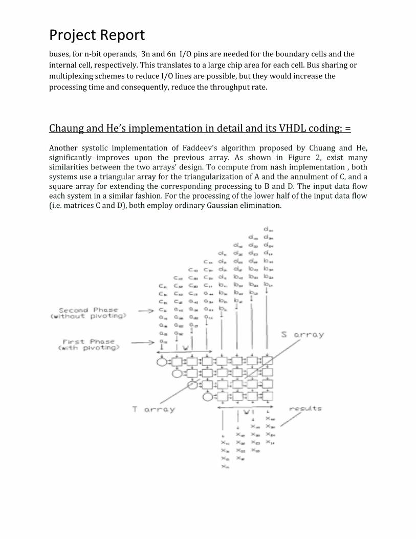
Another systolic implementation of Faddeev's algorithm proposed by Chuang and He, significantly improves upon the previous array. As shown in Figure 2, exist many similarities between the two arrays' design. To compute from nash implementation , both systems use a triangular array for the triangularization of A and the annulment of C, and a square array for extending the corresponding processing to B and D. The input data flow each system in a similar fashion. For the processing of the lower half of the input data flow (i.e. matrices C and D), both employ ordinary Gaussian elimination.

Project Report However, Chuang and He's system processes the upper half of the input data flow (i.e. matrices A and B) using Gaussian elimination with neighbor pivoting instead of the Givens transform.1 9 Hence, while numerical accuracy is somewhat inferior, this implementation is less expensive in terms of processing time and hardware complexities. Because the square root operation is not used, the array avoids the bottleneck problem created by the boundary cells of the Nash's array. And since the rightward data flow essentially consists of only one operand, Mout the pin counts of boundary cell and internal cell are correspondingly reduced to 3n and 4n, respectively. Since it is obvious that different phases processing are required for the upper half and the lower half of the data flow, two separate sets of micro programs for boundary cells and internal cells are needed, as shown in Figure 9 and 10. The first set, the pivoting functions, Performs Gaussian elimination with neighbor pivoting on A and B, while the second set, the non-pivoting functions, performs regular Gaussian elimination on C and D and is essentially the same as the functions of Nash cells in Figure 7. As the data flow is pipelined through the array, each boundary cell stores an input data element and sends a multiplier Mou t rightwards to modify the input data that o u enter the internal cells of the same row.

Here in figure shown first phase working.

Project Report Along with each Mout it generates a one-bit boolean value Vout to signal whether pivoting is needed. Each internal cell stores a data value arriving from the top and passes downward all the following data after modification. Mout and Vout remain unchanged as they travel rightwards through the array. For an input column of length and width 2n data elements, the output will be a matrix of order n emerging from the bottom of square array. It can be seen that when the system matches the I/O bandwidth, 5n -1 steps are required to obtain C B + D and 4n steps are needed to solve a linear system of n equations.

Here it shown in second phase working.

Like in the Nash's implementation, the input data flow of this array can be continuous if additional control capabilities are used to individually switch each cell from pivoting to non-pivoting mode as required. As published, no technique was mentioned by the authors of both implementations to perform this switching; however, we can think of at least two different techniques to do this. One is to have the host or a dedicated controller generate the controls necessary for each individual cell, thus requiring a complex cell addressing scheme. Another is to tag control bits to input data elements which will then carry the control information with them throughout the array. This method assumes that the host, while generating the input data, will add the necessary control information to it. Its Down side is that it will force an enlargement of the I/O bandwidth between the host and the array. In the next chapter, it will be shown that a combination of the above mentioned technique will be used in our design. Thus, while having the advantages of both, it will avoid some of their inefficiencies.

Project Report Difficulties chased in this project: =

In this project first we understand Faddeev’s algorithm and real difficulties I faced in Nash

implementation first it is really hard to implement square root operation and compile it

after that It take more cycle period than regular one. It gives simulation error when there is

square root operation with negative values. It is really hard to implement this architecture

in VHDL.

Chuang and He’s implementation is quite simple as comparied to Nash implementation it

has less pins and it does not involve any hard mathematical stuff. But still It has some

timing problems with it that I have faced with it.

Conclusion: =

In this home works and project I have good experience to implementing Nash and Chuang

algorithm. There is lot of difficulties with Nash algorithm and it gives simulation errors.

Chuang and He’s algorithm are simple and can be simulate. But still in this also there is

some timing issue. Although these algorithms are good and working fine this are not

practical means they are not synthesizable.

Project Report VHDL code for Nash Implementation: =

Here we have given code for packet we have build for 2*2 matrix.

-- In this program Packet for NASH's Implimentation has given.

LIBRARY ieee;

USE ieee.std_logic_1164.ALL;

USE ieee.std_logic_arith.ALL;

USE ieee.std_logic_unsigned.ALL;

USE ieee.numeric_std.ALL;

USE ieee.math_real.ALL;

PACKAGE cell IS

COMPONENT delay

PORT(CLK : in std_logic;

D:in real;

Q:out real);

end COMPONENT;

COMPONENT cell_circular

PORT(Xin:in real; --CLK : in std_logic;

Cout,Sout:out real);

end COMPONENT;

COMPONENT cell_square

PORT(Xin,Cin,Sin: real; --CLK : in std_logic;

Xout,Cout,Sout:out real);

end COMPONENT;

end cell;

--frist we define here delay cell

LIBRARY ieee;


Entity delay is

PORT(CLK : in std_logic;

D:in real;

Q:out real);

end delay;

architecture delay_arch of delay is

begin

process(D)

begin

if (clk'event) and (clk = '1') then

Q <= D;

end if;

Project Report end process;

end delay_arch;

-- This procedure represents the execution code of NASH's Systolic Array

for Boundry cell.

-- for our simliicity we name it as cell_circular.

LIBRARY ieee;






entity cell_circular is

PORT(Xin:in real ; --clk : in std_logic;

Cout,Sout:out real);

end cell_circular;

architecture cell_circular_arch of cell_circular is

signal T,S1,S2,S3: real:=0.0;

begin

process (Xin)

variable rl: real:= 0.0;

variable Nl: integer := 0;

constant g: integer := 2;

constant h: real := 0.0;

begin


if (Nl < g) then

if Xin = h then

Cout <= 1.0;

Sout <= 0.0;

rl := 0.0;

else

S1 <= rl*rl;

S2 <= Xin*Xin;

S3 <= S1+S2;

T <= SQRT(S3);

Cout <= rl/T;

Sout <= Xin/T;

rl := T;

end if;

Nl := Nl+1;

else

Cout <= Xin/rl;

Sout <= 0.0;

end if;

end if;

end process;

end cell_circular_arch;


for Internal cell.

Project Report -- For our simplicity we name it as CELL_square.

Library ieee;






entity cell_square is

PORT(Xin,Cin,Sin: real; --CLK : in std_logic;

Xout,Cout,Sout:out real);

end cell_square;

architecture cell_square_arch of cell_square is

signal S5,S7,S8: real;

begin

process (Xin,Cin,Sin)

variable rl: real:= 0.0;

variable N: integer := 0;


begin


if N < g then

Cout <= Cin;

Sout <= Sin;

S5 <= (-Sin*rl);

--S6 <= (Cin*Xin);

Xout <= S5 ;

S7 <= (Cin*rl);

S8 <= (Sin *Xin);

rl := S7 + S8;

N := N+1;

else

Xout <= Xin-(Cin*rl);

Sout <= 0.0;

end if;

end if;

end process;

end cell_square_arch;

Here we are now defining systolic array for Nash Implementation.

-- First we are define cells we gonna to use and we map them according to

our requirment

LIBRARY ieee;






Project Report

LIBRARY WORK;

USE WORK.CELL.ALL;

ENTITY SYS2is2 IS

PORT(clk: std_logic;

A : in real;

B : in real;

C : in real;

E : in real;

X,Y : out real);

end sys2is2;

Architecture A of sys2is2 is

signal T,S1,S2,S3,S4,S5,S7,S8: real:=0.0;

signal Sout1,Cout1,Sout2,Cout2,Sout3,Cout3,Sout4,Cout4: real:=0.0;

SIGNAL Sout5,Cout5,Sout6,Cout6,Sout7,Cout7: real:=0.0;

SIGNAL Xout2,Xout3,Xout4,Xout5,Xout6,Xout7: real:=0.0;

signal Q1,Q2,Q3,Q4,Q5,Q6,Q7: real:=0.0;

begin

process (A,B,C,E,CLK)

BEGIN


delay1 : delay port map (B,Q1);

delay2 : delay port map (C,Q2);

delay3 : delay port map (E,Q3);

delay4 : delay port map (Q2,Q4);



cell1 : cell_circular port map( A,Sout1,Cout1);

cell2 : cell_square port map (Q1,Sout1,Cout1,Xout2,Sout2,Cout2);



cell5 : cell_circular port map(Xout2,Sout5,Cout5);

cell6 : cell_square port map(Xout3,Sout5,Cout5,Xout6,Sout6,Cout6);

cell7 : cell_square port map(Xout4,Sout6,Cout6,Xout7,Sout7,Cout7);

delay7 : delay port map (Xout6,Q7);

X <= Q7;

y <= Xout7;

END IF;

end process;

end A;

Here we define test bench for Nash implementation. LIBRARY ieee;





Project Report USE ieee.math_real.ALL;

entity testsys is

end testsys;

use work.all;

architecture test of testsys is

component SYS2is2

PORT(CLK: IN std_logic;

A : in real;

B : in real;

C : in real;

E : in real;

X,Y : out real);

end component;

SIGNAL CLOCKCYCLE:NATURAL:=0;

SIGNAL CLK : STD_LOGIC;

signal A,B,C,E,Y,X: real;

signal Sout1,Cout1,Sout2,Cout2,Sout3,Cout3,Sout4,Cout4: real:=0.0;

SIGNAL Sout5,Cout5,Sout6,Cout6,Sout7,Cout7: real:=0.0;

SIGNAL Xout2,Xout3,Xout4,Xout5,Xout6,Xout7: real:=0.0;

signal Q1,Q2,Q3,Q4,Q5,Q6,Q7: real:=0.0;

signal T,S1,S2,S3,S4,S5,S6,S7,S8: real:=0.0;

constant clockperiod: time := 100ns;

begin

uut: SYS2is2 port map (CLK,A,B,C,E,X,Y);

clock: process

BEGIN

CLOCKCYCLE<=CLOCKCYCLE + 1;

CLK <= '1';

wait for 50ns;

CLK <= '0';

wait for 50ns;

end process clock;

simulus: process

begin

--WAIT FOR clockperiod;

A<=2.0;B<=-1.0;C<=1.0;E<=2.0;

WAIT FOR clockperiod;

A<=-1.0;B<=0.0;C<=3.0;E<=1.0;


A<=1.0;B<=-2.0;C<=0.0;E<=4.0;


A<=0.0;B<=-7.0;C<=-2.0;E<=1.0;


--A<=0.0;B<=0.0;C<=0.0;E<=0.0;


--A<=0.0;B<=0.0;C<=0.0;E<=0.0;


--A<=0.0;B<=0.0;C<=0.0;E<=0.0;


Project Report --A<=0.0;B<=0.0;C<=0.0;E<=0.0;


--A<=0.0;B<=0.0;C<=0.0;E<=0.0;


WAIT;

end process simulus;

end test;

VHDL code for Chaung and He’s Implementation: =

Here we define packet for chuang and He’s implementation

-- In this program Packet for NASH's Implimentation has given.

LIBRARY ieee;






PACKAGE cell_chang IS

COMPONENT delay_chang

PORT(--CLK : in std_logic;

D:in integer;

Q:out integer);

end COMPONENT;

COMPONENT cell_circular_chang

PORT(Xin:in integer;

Mout: out integer; Vout:in integer );

end COMPONENT;

COMPONENT cell_square_chang

PORT(Xin,Min: integer; Vin : in integer;

Xout,Sout:out integer;Vout: out integer);

Project Report end COMPONENT;

end cell_chang;

--frist we define here delay cell

LIBRARY ieee;


Entity delay_chang is

PORT(--CLK : in std_logic;

D:in integer;

Q:out integer);

end delay_chang;

architecture delay_arch of delay_chang is

begin

--process(D)

--begin

--if (clk'event) and (clk = '1') then

Q <= D;

--end if;

--end process;

end delay_arch;


for Boundry cell.

-- for our simliicity we name it as cell_circular.

LIBRARY ieee;






entity cell_circular_chang is

PORT(Xin:in integer ;

Mout:out integer; Vout: out integer);

end cell_circular_chang;

architecture cell_circular_arch of cell_circular_chang is

begin

process (Xin)

variable Xc: integer:= 0;

variable Nl: integer := 0;


constant h: integer := 0;

begin


if (Nl < g) then

if Xin >= Xc then

Vout <= 1;

Project Report if Xin/=h then

Mout <= (-Xc/Xin);

else

Mout<=0;

Xc := Xin;

end if;

else

Vout<=0;

Mout<=(-Xin/Xc);

end if;

else

Mout<=(-Xin/Xc);

end if;

end process;

end cell_circular_arch;


for Internal cell.

-- For our simplicity we name it as CELL_square.

Library ieee;






entity cell_square_chang is

PORT(Xin,Min: integer; Vin : in integer;

Xout,Sout:out integer; Vout: out integer);

end cell_square_chang;

architecture cell_square_arch of cell_square_chang is

begin

process (Xin,Min,Vin)

variable Xs: integer:= 0;

variable N: integer := 0;


begin


if N < g then

if Vin = 1 then

Xout<= Xs + (Min*Xin);

Xs:=Xin;

else

Xout<=Xin+(Min*Xs);

end if ;

else

Xout<=Xin+(Min*Xs);

end if;

end process;

end cell_square_arch;

Project Report

Here we define systolic architecture for Chuang and He’s implementation.

-- First we are define cells we gonna to use and we map them according to

our requirment

LIBRARY ieee;





--USE ieee.math_real.ALL;

LIBRARY WORK;

USE WORK.CELL_chang.ALL;

ENTITY SYS_chang IS

PORT(clk: std_logic;

A : in integer;

B : in integer;

C : in integer;

E : in integer;

X,Y : out integer);

end sys_chang;

Architecture A of sys_chang is

signal Mout1,Mout2,Mout3,Mout4,Mout5,Mout6,Mout7: integer:=0;

SIGNAL Vout1,Vout2,Vout3,Vout4,Vout5,Vout6,Vout7: integer:=0;

SIGNAL Xout2,Xout3,Xout4,Xout5,Xout6,Xout7: integer:=0;

signal Q1,Q2,Q3,Q4,Q5,Q6,Q7: integer:=0;

begin

--process (A,B,C,E,CLK)

--BEGIN


delay1 : delay_chang port map (B,Q1);

delay2 : delay_chang port map (C,Q2);

delay3 : delay_chang port map (E,Q3);

delay4 : delay_chang port map (Q2,Q4);



cell1 : cell_circular_chang port map( A,Mout1,Vout1);

cell2 : cell_square_chang port map

(Q1,Mout1,Vout1,Xout2,Mout2,Vout2);





cell5 : cell_circular_chang port map(Xout2,Mout5,Vout5);


(Xout3,Mout5,Vout5,Xout6,Mout6,Vout6);


(Xout4,Mout6,Vout6,Xout7,Mout7,Vout7);

Project Report delay7 : delay_chang port map (Xout6,Q7);

X <= Q7;

y <= Xout7;

--END IF;

--end process;

end A;

Test bench for Chuang and He’s Implementation.

LIBRARY ieee;






entity testsys_chang is

end testsys_chang;

LIBRARY WORK;

USE WORK.CELL_chang.ALL;

architecture test of testsys_chang is

component SYS_chang

PORT(CLK: IN std_logic;

A : in integer;

B : in integer;

C : in integer;

E : in integer;

X,Y : out integer);

end component;

SIGNAL CLOCKCYCLE:NATURAL:=0;

SIGNAL CLK : STD_LOGIC;

signal A,B,C,E,Y,X: integer;

signal Mout1,Mout2,Mout3,Mout4,Mout5,Mout6,Mout7: integer:=0;

SIGNAL Vout1,Vout2,Vout3,Vout4,Vout5,Vout6,Vout7: integer:=0;

SIGNAL Xout2,Xout3,Xout4,Xout5,Xout6,Xout7: integer:=0;

signal Q1,Q2,Q3,Q4,Q5,Q6,Q7: integer:=0;

constant clockperiod: time := 100ns;

begin

uut: SYS_chang port map (CLK,A,B,C,E,X,Y);

clock: process

BEGIN

CLOCKCYCLE<=CLOCKCYCLE + 1;

CLK <= '1';

wait for 50ns;

CLK <= '0';

wait for 50ns;

end process clock;

Project Report simulus: process

begin



A<=2;B<=1;C<=1;E<=2;

END IF;



A<=1;B<=0;C<=3;E<=1;

END IF;



A<=1;B<=2;C<=0;E<=4;

END IF;



A<=0;B<=7;C<=2;E<=1;

END IF;



A<=0;B<=0;C<=0;E<=0;

END IF;



A<=0;B<=0;C<=0;E<=0;

END IF;



A<=0;B<=0;C<=0;E<=0;

END IF;



A<=0;B<=0;C<=0;E<=0;

END IF;



A<=0;B<=0;C<=0;E<=0;

END IF;


WAIT;

end process simulus;

end test;

Project Report Reference: =

1. Wikipedia

2. Class notes

3. A theses : A new General purpose Systolic Array for

Matrix Computations—Van Dinh Le.

ece 590: digital systems design using hardware description...

Documents