ECE 541 - RANDOM SIGNAL PROCESSING LECTURE NOTES

MAJEED M. HAYAT

Date: July 25, 2004.

1

2 MAJEED M. HAYAT

Contents

1. Set 1: Fundamentals of Probability 6

1.1. Experiments 6

1.2. Outcomes and the Sample Space 6

1.3. Events 6

1.4. Random Variables 9

2. Set 2: Fundamentals of Probability, Continued 11

2.1. Probability Measure 11

2.2. Expectation 13

3. Lecture 1: 08/25/03 16

3.1. Definition of Sample Space, Events and Random Variables 16

3.2. Sub-algebras 17

4. Lecture 2: 08/27/03 18

4.1. Set Theory Notation 18

4.2. Random Variables 19

5. Lecture 3: 09/03/2003 21

5.1. Random Variables 21

5.2. Properties of Random Variables 21

5.3. Measure 22

5.4. Expectation 23

6. Lecture 4: 09/08/2003 24

6.1. Expectation 24

6.2. Distributions 25

6.3. Distribution Function 25

6.4. Density Functions 26

7. Lecture 5: 09/10/2003 27

7.1. Elementary Hilbert Space Theory 27

7.2. Schwarz Inequality 27

7.3. Triangle Inequality 27

7.4. Convex Sets 28

7.5. Orthogonality 28

8. Lecture 6: 09/15/03 29

8.1. Triangle Inequality 29

8.2. Notion of a Closed Set 29

8.3. Application 30

ECE 541 3

9. Lecture 7: 09/17/03 32

9.1. Minimum Distance Properties 33

9.2. Linearity 33

9.3. Properties of Conditional Expectation 33

10. Lecture 8: 09/22/03 35

11. Lecture 9: 09/29/03 37

11.1. Applications of Conditional Expectations: 37

12. Lecture 10: 10/01/03 38

13. Lecture 11: 10/06/03 40

13.1. Independence 40

13.2. Parameter Estimation 41

14. Lecture 12: 10/13/03 43

14.1. Parameter Estimation 43

14.2. Chebychev’s Inequality 43

14.3. Weak Law of Large Numbers 44

14.4. Maximum Likelihood Estimation 44

15. Lecture 13: 10/15/03 45

15.1. Maximum Likelihood Estimation 45

15.2. Linear Parameter Estimation 45

16. Lecture 14: 10/20/03 48

16.1. Example of MLE 48

16.2. Almost Sure Convergence 48

16.3. Another Type of Convergence of Random Sequences 48

16.4. Central Limit Theorem (CLT) 48

16.5. Inversion Lemma (Levy’s) 49

16.6. Back to Proof of CLT 49

17. Lecture 15: 10/22/03 50

17.1. Central Limit Theorem (CLT) 50

17.2. Taylor’s Theorem with a Remainder 50

17.3. Whitening Filter 51

18. Lecture 16: 10/27/03 52

18.1. Covariance Matrix 52

18.2. Whitening of Correlated Data 52

18.3. Simultaneous Diagonalization of Two Covariance Matrices 53

18.4. Summary 53

4 MAJEED M. HAYAT

19. Lecture 17: 10/29/03 55

19.1. Random Processes 55

19.2. Wide Sense Stationary (WSS) 56

19.3. Example of Random Processes 56

20. Lecture 18: 11/03/03 58

20.1. Review 58

20.2. Brownian Motion 59

20.3. White Noise 59

21. Lecture 19: 11/05/03 60

21.1. White Noise 60

21.2. Independent Increment Hypothesis 60

21.3. Application of White Noise 61

21.4. Norton Model for Thermal Noise 61

22. Lecture 20: 11/10/03 63

22.1. Practical Interpretation 64

22.2. Connection between RX(z) and SX(ω) 64

22.3. Response of LTI Systems to WSS Stochastic Process 66

23. Lecture 21: 11/12/03 68

23.1. Linear Systems Response 68

24. Lecture 22: 11/17/03 73

24.1. Fact about Gaussian r.v.’s 73

24.2. Conditional Expectations 73

24.3. Poisson Process 73

24.4. Hazard or Failure Rates 75

25. Lecture 23: 11/19/03 77

25.1. Linear Estimation: Discrete Case 77

25.2. Linear Estimation: Continuous Case 78

26. Lecture 24: 11/24/03 82

26.1. Linear Filtering 82

26.2. Causal Wiener Filtering 82

27. Lecture 25: 11/26/03 86

27.1. Spectral Factorization 86

27.2. Optimal Linear Prediction 87

27.3. Smoothing 88

27.4. Markov Chains 88

ECE 541 5

28. Lecture 26: 12/01/03 90

28.1. Linear Prediction 90

28.2. Markov Chains 92

28.3. Martingales 94

28.4. Markov Chains 94

29. Lecture 27: 12/03/03 95

29.1. Gambler’s Ruin Problem 95

30. Lecture 28: 12/08/03 100

30.1. Sampling Theorem for Bandlimited Stochastic Processes 100

30.2. Stochastic Sampling Theorem 103

References 105

6 MAJEED M. HAYAT

1. Set 1: Fundamentals of Probability

1.1. Experiments. The most fundamental component in probability theory is the existence of a

physical or abstract “experiment,” whose “outcome” is revealed when the experiment is completed.

Probability theory aims to provide the tools that will enable us to assess the likelihood of an outcome,

or more generally, the likelihood of any outcome from a collection of outcomes. Let us consider the

following example:

Example 1. Shooting a single dart: Consider shooting a single dart at a target (board) represented

by the unit closed disc, D, which is centered at the point (0, 0). We write D = (x, y) ∈ <2 :

x2 + y2 ≤ 1. Here, < denotes the set of real numbers (same as (−∞,∞)), and <2 is the set of all

points in the plane ( <2 = <×<, where × denotes the Cartesian product of sets). We read the above

description of D as “the set of all points (x, y) in <2 such that (or with the property) x2 + y2 ≤ 1.

1.2. Outcomes and the Sample Space. Now we define what we mean by an outcome: An

outcome can be a “miss target,” in which case the dart misses the board entirely, or it can be its

location in the case that it does not miss the board. Note that we intentionally do not care where

the dart lands as long as it missed the board. (The definition of an outcome is totally arbitrary and

therefore it is not unique for any experiment.) Mathematically, we form what is called the sample

space as the set containing all possible outcomes. If we call this set Ω, then Ω=“miss”∪D, where

the symbol ∪ denotes set union (we say x ∈ A ∪ B if and only if x ∈ A or x ∈ B). We write ω ∈ Ω

to denote a specific outcome from the sample space Ω. For example, ω = “miss,” ω = (0, 0), and

ω = (0.1, 0.2) are possible outcomes; however, according to our definition of an outcome, ω cannot

be (1,1).

1.3. Events. An event is a collection of outcomes, that is, a subset in Ω. Such a subset can be

associated with a question that we may ask about the outcome of the experiment and whose answer

can be determined after the outcome is revealed. For example, the question: “Q1: Did the dart

land within 0.5 of the bull’s eye?” can be associated with the subset of Ω (or event) given by

E = (x, y) ∈ <2 : x2 + y2 ≤ 1/4. We would like to call the set E an event. Now consider the

complement of Q1, that is: Q2: “Did the dart not land within 0.5 of the bull’s eye?” with which

we can associate the event Ec, were the superscript “c” denotes set complementation (relative to

Ω). Namely, Ec = Ω\E, the set of outcomes (or points or members) of Ω that are not already in E.

The notation “\” represents set difference (or subtraction). Note that Ec = (x, y) ∈ <2 : x2 + y2 >

1/4∪“miss”. The point here is that if E is an event, then we would want Ec to qualify as an

event as well since we would like to be able to ask the logical negative of any question. In addition,

we would also like to be able to form a logical “or” of any two questions about the experiment

outcome. Thus, if E1 and E2 are events, we would like their union to also be an event. For example,

ECE 541 7

for each n = 1, 2, . . ., define the subset En = (x, y) ∈ <2 : x2 + y2 ≤ 1 − 1/n and let⋃∞

n=1 En be

their countable union. (Notation: ω ∈ E if and only if x ∈ En for some n.) It is not hard to see

(prove it) that E = (x, y) ∈ <2 : x2 + y2 < 1, which corresponds to the valid question “did the

dart land inside the board?” Thus, we would want E (which is the countable union of events) to be

an event as well.

Finally, we should be able to ask whether or not the experiment was conducted or not, that is,

we would like to label the sample space Ω as an event as well. With this (hopefully) motivating

introduction, we proceed to formally define what we mean by events.

Definition 1. A collection F of subsets of Ω is called a σ − algebra (read sigma algebra) if:

(1) Ω ∈ F(2)

⋃∞n=1 En whenever En ∈ F , n = 1, 2, . . .

(3) Ec ∈ F whenever E ∈ F

If F is a σ-algebra, then its members are called events.

Consequences (prove all of them):

(1) ∅ ∈ F (prove it).

(2)⋂∞

n=1 En ∈ F whenever En ∈ F , n = 1, 2, . . . (Prove it). Here, the countable intersection⋂∞

n=1 En is defined as follows: ω ∈ ⋂∞n=1 En if and only if x ∈ En for all n.

(3) A\B ∈ F whenever A,B ∈ F .

Members of a σ-algebra are also called measurable sets.

Definition 2. Let Ω be a sample space and let F be a σ-algebra of events. We call the pair (Ω,F)

a measurable space.

Definition 3. A collection D of subsets of Ω is called a sub- σ-algebra of D if

(1) D ⊂ F (this means that if A ∈ D, then automatically A ∈ F ).

(2) D is itself a σ-algebra.

Example 2. ∅,Ω is a sub-σ-algebra of any other σ-algebra.

Example 3. The power set of Ω, which is the set of all subsets of Ω, is a σ-algebra. In fact it is a

maximal σ-algebra in a sense that it contains any other σ-algebra. The power set of a set Ω is often

denoted by 2Ω.

Interpretation: Once again, we emphasize that it would be meaningful to think of a σ-algebra as a

collection of all valid questions that one may ask about an experiment. The collection has to satisfy

certain self-consistency rules, dictated by the requirements for a σ-algebra, but what we mean by

“valid” is really up to us as long as the self-consistency rules are met.

8 MAJEED M. HAYAT

Generation of σ-algebras: Let M be a collection of events (not necessarily a σ-algebra). This

collection could be a collection of certain events of interest. For example, M = “miss”, (x, y) ∈<2 : 1/4 ≤ x2 + y2 = 1/2 in the dart experiment. The question is can we construct a minimal

σ-algebra that contains M? If such a σ-algebra exists, call it FM, then it must possess the following

properties:

(1) M ⊂ F(2) If D is another σ-algebra containing M, then necessarily FM ⊂ D. Hence FM is minimal.

The following Theorem states that there is such a minimal σ-algebra.

Theorem 1. Let M be a collection of events, then there is a minimal σ-algebra containing M.

Before we prove the Theorem let us look at an example.

Example 4. Suppose that Ω = (−∞,∞), and M = (−∞, 1), (0,∞). It is easy to see (as done in

class) that FM = ∅,Ω, (−∞, 1), (0,∞), (0, 1), (−∞, 0], [1,∞), (−∞, 0][1,∞). Explain where each

member is coming from?

Proof of Theorem: Let KM be the collection of all σ-algebras that contain M. We observe

that such a collection is not empty since at least it contains the power set 2Ω. Let us label each

member of KM by an index α, namely Dα , where α ∈ I, where I is some index set. Define

FM =⋂

α∈I Dα. We need to show that 1) FM is a σ-algebra containing M, and 2) that FM is a

minimal σ-algebra. Note that each Dα contains Ω, thus FM contains Ω. If A ∈ FM, then A ∈ Dα,

for each α ∈ I. Thus, Ac ∈ Dα, for each α ∈ I (since each Dα is a σ-algebra) which implies that

Ac ∈ ⋂α∈I Dα. Now suppose that A1, A2, . . . ∈ FM. Then, we know that A1, A2, . . . ∈ Dα, for each

α ∈ I. Moreover,⋃∞

n=1 An ∈ Dα, for each α ∈ I (again, since each Dα is a σ-algebra) and thus⋃∞

n=1 An ∈ ⋂α∈I Dα. This completes proving that FM is a σ-algebra. Now suppose that F ′M is

another σ-algebra containing M, we will show that FM ⊂ F ′M. First note that since KM is the

collection of all σ-algebras containing M, then it must be true that F ′M = Dα∗ for some α∗ ∈ I. If

A ∈ FM, then necessarily A ∈ Dα∗ = F ′M, which establishes that FM ⊂ F ′

M. This completes the

proof of the theorem.

Example 5. Let U be the collection of all open sets in <. Then, according to the above theorem,

there exists a minimal σ-algebra containing U. This σ-algebra is called the Borel σ-algebra, B, and

its elements are called the Borel subsets of <. Note that by virtue of set complementation, union and

intersection, B contains all closed sets, half open intervals, their countable unions, intersections,

and so on.

ECE 541 9

(Reminder: A subset U in < is called open if for every x ∈ <, there exists a disc centered at

x which lies entirely in U . Closed sets are defined as complements of open sets. These definitions

extend to <n in a straightforward manner.)

Restrictions of σ-algebras: Let F be a σ-algebra. For any measurable set U , we define F ∩U as

the collection of all intersections between U and the members of F , that is F∩U = V ∩U : V ∈ F.It is easy to show that F ∩ U is also a σ-algebra, which is called the restriction of F to U . (See

Exercise 2 in HW#1 and its solution for an example.)

Example 6. Back to the dart experiment: What is a reasonable σ-algebra for this experiment? I

would say any such σ-algebra should contain all the Borel subsets of D and the “miss” event.

So we can take M = “miss”,B ∩ D. It is easy to check that in this case FM = ((B ∩ D) ∪“miss”) ∪ (B∩D), where for any σ-algebra F and any measurable set U , we define F ∪U as the

collection of all unions between U and the members of F , that is F ∪ U = V ∪ U : V ∈ F. Note

that F ∪U is not always a σ-algebra (contrary to F ∩U), but in this example it is because “miss”is the complement of D.

1.4. Random Variables. Motivation: Recall the dart experiment, and define the following trans-

formation on the sample space:

X: Ω → < defined as

X(ω) =

1, if ω ∈ D

0, if ω = “miss”

where D = (x, y) ∈ <2 : x2+y2 ≤ 1. Consider the sets of outcomes that we can identify if we knew

that X fell in the interval (−∞, r). More precisely, we want to identify ω ∈ Ω : X(ω) ∈ (−∞, r),or equivalently, the set X−1((−∞, r)), which is the inverse image of the set (−∞, r). It is easy to

see that:

For r < 0, X−1((−∞, r)) = ∅,for 0 ≤ r < 1, X−1((−∞, r)) = “miss”and for 1 ≤ r < ∞, X−1((−∞, r)) = Ω.

Note that in each case, X−1((−∞, r)) is an event (i.e., a member of F for this experiment). Now

let M = ∅, “miss”,Ω, then it is easy to check that FM = ∅, “miss”,Ω, D, which can be

intuitively identified as the set of all events that X can convey about the experiment. In particular,

FM consists of precisely those events whose occurrence can be determined through our observation

of the value of X. In other words, FM is the “information” that X can provide about the outcome of

the experiments. Note that ∅, “miss”,Ω, D is much smaller than the original σ-algebra F , which

was ((B∩D)∪“miss”)∪ (B∩D). Clearly, ∅, “miss”,Ω, D ⊂ ((B∩D)∪“miss”)∪ (B∩D).

10 MAJEED M. HAYAT

Thus, X only partially informs us of the true outcome of the experiment; albeit, whatever X conveys

about the experiment is an event.

Motivated by this example, we proceed to define what we mean by a random variable.

Definition 4. Let (Ω,F) be a measurable space. A transformation X : Ω → < is said to be

F-measurable if for every r ∈ <, X−1((−∞, r)) ∈ F . In such a case, X is called a random variable.

Now let X be a random variable and consider the collection of events M = ω ∈ Ω : X(ω) ∈(−∞, r), r ∈ <, which can also be written as X−1((−∞, r)), r ∈ <. As before, let FM be

the minimal σ-algebra containing M. Then, FM is the “information” that the random variable X

conveys about the experiment. We define such a σ-algebra from this point on as σ(X), the σ-algebra

generated by the random variable X. In the above example of X, σ(X) = ∅, “miss”,Ω, D. See

Exercise 3 in HW#1 for another example of σ(X).

Facts about Measurable Transformations: Let (Ω,F) be a measurable space. The following

statements are equivalent:

(1) X is a measurable transformation.

(2) X−1((−∞, r]) ∈ F . (we proved this in class)

(3) X−1((r,∞)) ∈ F .

(4) X−1([r,∞)) ∈ F .

(5) X−1((a, b)) ∈ F for all a ≤ b.

(6) X−1([a, b)) ∈ F for all a ≤ b.

(7) X−1([a, b]) ∈ F for all a ≤ b.

(8) X−1((a, b]) ∈ F for all a ≤ b.

(9) X−1(B) ∈ F for all B ∈ B.

Using (9), we can equivalently define σ(X) as X−1(B) : B ⊂ B, which can be directly shown

to be a σ-algebra (prove it).

ECE 541 11

2. Set 2: Fundamentals of Probability, Continued

2.1. Probability Measure.

Definition 5. Consider the measurable space (Ω,F). A set function, P , mapping F into < is called

a probability measure if

(1) P (E) ≥ 0.

(2) P (Ω) = 1.

(3) If E1, E2, . . . ∈ F and if Ei ∩ Ej = ∅ when i 6= j, then P (⋃∞

n=1 En) =∑∞

n=1 P (En).

The following properties follow directly from the above definition.

Property 1. P (∅) = 0.

Proof. Put E1 = Ω, E2 = . . . = En = ∅ in (3) and use (2) to get 1 = P (Ω) = P (Ω ∪ ∅ ∪ ∅ ∪ . . .) =

P (Ω) +∑∞

n=2 P (φ) = 1 +∑∞

n=2 P (φ). Thus,∑∞

n=2 = 0, which implies that P (∅) = 0 since P (∅) ≥ 0

according to (1).

Property 2. If E1, E2, . . . , En ∈ F and if Ei∩Ej = ∅ when i 6= j, then P (⋃n

i=1 Ei) =∑n

i=1 P (En).

Proof. Put En+1 = En+2 = . . . = ∅ and the result will follow from 3 since P (∅) = 0 (from Property

2)

Property 3. If E1, E2 ∈ F and E1 ⊂ E2, then P (E1) ≤ P (E2).

Proof. Note that E1 ∪ E2\E1 = E2 and E1 ∩ E2\E1 = ∅. Thus, by Property 2 (use n = 2),

P (E2) = P (E1) + P (E2\E1) ≥ P (E1), since P (E2\E1) ≥ 0.

Property 4. If A1 ⊂ A2 ⊂ A3 . . . ∈ F , then

(1) limn→∞

P (An) = P (

∞⋃

n=1

An).

Proof. Put B1 = A1, B2 = A2\A1, . . . , Bn = An+1\An, . . .. Then, it is easy to check that⋃∞

n=1 =⋃∞

n=1 Bn and⋃m

n=1 =⋃m

n=1 Bn for any m ≥ 1, and that Bi ∩ Bj = ∅ when i 6= j. Hence,

P (⋃n

i=1 Ai) =∑n

i=1 P (Bi) and P (⋃∞

i=1 Ai) =∑∞

i=1 P (Bi). But,⋃n

i=1 Ai = An, so that P (An) =∑n

i=1 P (Bi). Now since∑n

i=1 P (Bi) converges to∑∞

i=1 P (Bi), we conclude that P (An) converges

to∑∞

i=1 P (Bi), which is equal to P (⋃∞

i=1 Ai) as shown above.

Property 5. If A1 ⊃ A2 ⊃ A3 . . ., then limn→∞ P (An) = P (⋂∞

n=1 An).

Proof. See HW#2.

The triplet (Ω,F , P ) is called a probability space.

12 MAJEED M. HAYAT

Example 7. Recall the dart experiment. We now define P on (Ω,F). Assign P (“miss”) = 0.5,

and for A ∈ D ∩ B, assign P (A) = area(A)/2π. It is easy to check that P defines a probability

measure. (For example, P (Ω) = P (D ∪ “miss”) = P (D) + P (“miss”) = area(D)/2π + 0.5 =

0.5 + 0.5 = 1. Check the other requirements as an exercise.)

Distributions: Consider a probability space (Ω,F , P ), and consider a random variable X defined

on it. Up to this point, we have developed a formalism that allows us to as questions of the form

“what is the probability that X assumes a value in a Borel set B?” Symbolically, this is written as

P (ω ∈ Ω : X(ω) ∈ B), or for short, PX ∈ B with the understanding that the set X ∈ B is an

event (i.e., member of F). Answering all the questions of the above form is tantamount to assigning

a number in the interval [0,1] to every Borel. Thus, we can think of a mapping from B into [0,1],

whose knowledge will provide an answer to all the questions of the form described earlier. We call

this mapping the distribution of the random variable X, and it is denoted by µX . Formally, we have

µX : B → [0, 1] according to the rule µX(B) = PX ∈ B, B ∈ B.

Proposition 1. µX defines a measure on B.

Proof. See HW#4.

Distribution Functions: Recall from your undergraduate probability that we often associate with

each random variable a distribution function, defined as FX(x) = PX ≤ x. This function can

also be obtained from the distribution of X, µX , by evaluating µX at B = (−∞, x], which is a Borel

set. That is, FX(x) = µX((−∞, x]).

Property 6. FX is nondecreasing.

Proof. For x1 ≤ x2, (−∞, x1] ⊂ (−∞, x2] and = µX((−∞, x1]) ≤ µX((−∞, x2]) since µX is a

probability measure (see Property 3 above).

Property 7. limx→∞ FX(x) = 1 and limx→−∞ FX(x) = 0.

Proof. Note that (−∞,∞) =⋃∞

n=1(−∞, n] and by Property 4 above, limn→∞ µX((−∞, n]) =

µX(⋃∞

n=1(−∞, n]) = µX((−∞,∞)) = 1 since µX is a probability measure. Thus we proved that

limn→∞ FX(n) = 1. Now the same argument can be repeated if we replace the sequence n by any in-

creasing sequence xn. Thus, limxn→∞ FX(xn) = 1 for any increasing sequence xn, and consequently

limx→∞FX(x) = 1.

The proof of the second assertion is left as an exercise.

Property 8. FX is right continuous, that is, limx↓y FX(x) = FX(y).

ECE 541 13

Proof. Note that FX(y) = µX((−∞, y]), and (−∞, y] =⋃∞

n=1(−∞, y + n−1]. So, by Property 4

above, limn→∞ µX((−∞, y + n−1]) = µX(⋂∞

n=1(−∞, y + n−1]) = µX((−∞, y]). Thus, we proved

that limn→∞ FX(y + n−1) = FX(y). In the same fashion, we can generalize the result to obtain

limn→∞ FX(y + xn) = FX(y) for any sequence for which xn ↓ 0. This completes the proof.

Example 8. (Problem 3.8 in the textbook) Let X be a uniformly-distributed random variable in [0,2].

Let the function g be as shown in Fig. 1 below. Compute the distribution function of Y = g(X).

1

1/2

1/2

FY(y)

y

1

1

g(x)

x1

Figure 1.

Solution: If y < 0, FY (y) = 0 since Y is nonnegative. If 0 ≤ y ≤ 1, FY (y) = P (X ≤y/2 ∪ X > 1 − y/2) = 0.5y + 0.5. Finally, if y > 1, FY (y) = 1 since Y ≤ 1. The graph of FY (y)

is shown above. Note that FY (y) is indeed right continuous.

2.2. Expectation. Recall that in an undergraduate probability course one would talk about the

expectation, average, or mean of a random variable. This is done by carrying out an integration (in

the Riemann sense) with respect to a probability density function. It turns out that the definition

of an expectation does require having a probability density function (pdf). It is based on a more or

less intuitive notion of an average. We will follow this general approach here and then connect it to

the usual expectation with respect to a pdf whenever the pdf exists. We begin by introducing the

expectation of a nonnegative random variable, and will generalize thereafter.

Consider a nonnegative random variable X, and for each n ≥ 1, we define the sum Sn =∑∞

i=1i

2n P i2n < X ≤ i+1

2n . We claim that Sn is nondecreasing. If this is the case (to be proven

shortly), then we know that Sn is either convergent (to a finite number) or Sn ↑ ∞. In any

case, we call the limit of Sn the expectation of X, and symbolically we denote as E[X]. Thus,

E[X] = limn→∞ Sn. To see the monotonicity of Sn, we follow Chow and Teicher [1] and observe

that

i2n < X ≤ i+1

2n = 2i2n+1 < X ≤ 2i+2

2n+1 = 2i2n+1 < X ≤ 2i+1

2n+1 ∪ 2i+12n+1 < X ≤ 2i+2

2n+1 ;thus,

Sn =∑∞

i=12i

2n+1 (P 2i2n+1 < X ≤ 2i+1

2n+1 + P 2i+12n+1 < X ≤ 2i+2

2n+1 )≤ 1

2n+1 P 12n+1 < X ≤ 2

2n+1 +∑∞

i=12i

2n+1 (P 2i2n+1 < X ≤ 2i+1

2n+1 + P 2i+12n+1 < X ≤ 2i+2

2n+1 )

14 MAJEED M. HAYAT

=∑∞

i=1,i oddi

2n+1 P i2n+1 < X ≤ i+1

2n+1 +∑∞

i=1,i eveni

2n+1 P i2n+1 < X ≤ i+1

2n+1 =∑∞

i=1i

2n+1 P i2n+1 < X ≤ i+1

2n+1 = Sn+1

If E[X] < ∞ , we say that X is integrable.

General Case: If X is any random variable, then we decompose it into two parts: a positive

part and a negative part. More precisely, let X+ = max(0, X) and X− = max(0,−X), then

clearly X = X+ + X−, and both of X+ and X− are nonnegative. Hence, we use our definition of

expectation for a nonnegative random variable to define E[X] = E[X+]E[X−] whenever E[X+] < ∞or E[X−] < ∞, or both. In cases where E[X+] < ∞ and E[X−] = ∞, or E[X−] < ∞ and

E[X+] = ∞, we define E[X] = −∞ and E[X] = ∞, respectively. Finally, E[X] is not defined

whenever E[X+] = E[X−] = ∞.

Special Case: Suppose that X is a binary random variable, that is, X(ω) = 1 if ω ∈ E and

IE(omega) = 0 otherwise, where E is some event. Then, E[X] = P (E). (Prove it.)

Notation and Terminology: E[X] is also written as∫

ΩX(ω)P (dω), which is called the

Lebesgue integral of X with respect to the probability measure P . Often, cumbersome notation

is avoided by writing∫

ΩXP (dω) or simply

∫

ΩXdP .

Linearity of Expectation: The expectation is linear, that is, E[aX+bY ] = aE[X]+bE[Y ]. This

can be seen, for example, by observing that any nonnegative random variable can be approximated

from below by functions of the form∑∞

i=1 xiIxi<X≤xj+1(ω), where for any event E, the random

variable IE(ω) = 1 if ω ∈ E and IE(ω) = 0 otherwise. (IE is called the indicator function of the set

E.) Indeed, we have seen such an approximation through our definition of the expectation. Namely,

if we define Xn(ω) =∑∞

i=1i

2n I i2n <X≤ i+1

2n (ω) , then it is easy to check that Xn(ω) → X(ω), as

n → ∞. In fact, E[X] was defined as limn→∞ E[Xn], where E[Xn] precisely coincides with Sn

described above [recall that E[IE(ω)] = P (E)]. Now to prove the linearity of expectations, we note

that if X and Y are random variables with defined expectations, then we can approximate them by

Xn and Yn, respectively. Also, Xn + Yn would approximate X + Y . Next, we observe that

E[Xn + Yn] = E[∑∞

i=1i

2n I i2n <X≤ i+1

2n (ω) +∑∞

i=1i

2n I i2n <Y ≤ i+1

2n (ω)]

= E[∑∞

j=1

∑∞i=1

i2n I i

2n <X≤ i+12n ∩ j

2n <Y ≤ j+12n (ω) +

∑∞j=1

∑∞i=1

j2n I i

2n <X≤ i+12n ∩ j

2n <Y ≤ j+12n (ω)]

= E[∑∞

j=1

∑∞i=1

i+j2n I i

2n <X≤ i+12n ∩ j

2n <Y ≤ j+12n (ω)].

But∑∞

j=1

∑∞i=1

i+j2n I i

2n <X≤ i+12n ∩ j

2n <Y ≤ j+12n (ω) = E[Xn + Yn].

ECE 541 15

Thus, we have shown that E[Xn]+E[Yn] = E[Xn +Yn]. Now take limits of both sides and use the

definition of E[X], E[Y ] and E[X + Y ] as the limits of E[Xn], E[Yn], and E[Xn + Yn], respectively,

to conclude that E[X] + E[Y ] = E[X + Y ]. The homogeneity property E[aX] = aE[X] can be

proved similarly.

Expectations in the Context of Distributions: Recall that for a nonnegative random vari-

able X, E[X] = limn→∞∑∞

i=1i

2n P i2n < X ≤ i+1

2n . But we had seen earlier that P i2n < X ≤

i+12n = µX(( i

2n , i+12n ]). So we can write

∑∞i=1

i2n P i

2n < X ≤ i+12n as

∑∞i=1

i2n µX(( i

2n , i+12n ]). We

denote the limit of the latter by∫

RxdµX , which is read as the Lebesgue integral of x with respect to

the probability measure µX . In summary, we have E[X] =∫

ΩXdP =

∫

RxdµX .

16 MAJEED M. HAYAT

3. Lecture 1: 08/25/03

3.1. Definition of Sample Space, Events and Random Variables.

Example 9. Shoot a dart at a target D, as depicted in Fig. 2. D = (x, y) ∈ <2 : x2 + y2 ≤ 1.Outcome:

(1) “miss”

(2) Give coordinates on the board D.

D

Figure 2.

The collection of all outcomes (if it is a set) is called a sample space associated with the experiment.

We call this set Ω and designate its members generically by ω (ω ∈ Ω), e.g., “miss” ∈ Ω, (0.5, π/4) ∈Ω, and (0, 0) ∈ Ω. We can group outcomes and form subsets of Ω, e.g., E1 = (x, y) ∈ <2 : x2+y2 ≤1/2 ⊂ Ω. Subsets of Ω are “called” events. We can think of E1 as a question: Q1 = “Is the point

within√

1/2 feet or less from the bullseye?” Q2 = “Did I miss?” E2 = “miss”. Clearly E2 ⊂ Ω

(subset of) because Ω = “miss”∪(x, y) ∈ <2 : x2 + y2 ≤ 1. Q3: Q1 or Q2? E3 = E1 ∪ E2.

Remark: If E1 and E2 are events then we want their union to be an event as well.

Qc1 = “Did we hit outside the disc of radius

√

1/2?”, where the “c” means set complementation.

Remark: If E is an event then we would like the complement Ec to be an event as well.

Consequence: If E1 and E2 are events, is E1 ∩ E2 an event? Yes. Because:

(1) E1 ∩ E2 = ∅ = ∴ E1 ∩ E2 is the impossible event (never occurs).

(2) E1 ∩ E2 = (Ec1 ∪ Ec

2)c

Let’s think of a legitimate collection of events. Call it F , e.g., F = E1, E2, E1∪E2, ∅, Ec1, E

c2,Ω, (E1∪

E2)c. F must have the following properties:

(1) ∅ ∈ F .

(2) If A,B ∈ F then A ∪ B ∈ F .

(3) If A ∈ F then Ac ∈ F .

We are not done: Suppose we take n = 1, 2, 3, . . .. An = (x, y) ∈ <2 : x2 + y2 ≤ 1/2 − 1/n. Note

that An ⊂ An+1. If An occurs then An+1 occurs.

ECE 541 17

An An+1

Figure 3.

Define: A∞ =⋃∞

n=1 An. By this we mean: if ω ∈ A then ω ∈ Ai for some i and if ω ∈ Ai for

some i, then ω ∈ A. A∞ = (x, y) ∈ <2 : x2 + y2 < 1/2, which is a logically legit event.

Formal Definition: Suppose that F is a collection of subsets of Ω, then we call F a σ-algebra

(of sets) if:

(1) Ω ∈ F .

(2) If A ∈ F , then Ac ∈ F .

(3) If A1, A2, . . . ∈ F , then⋃∞

n=1 An ∈ F .

3.2. Sub-algebras. We call a collection of events D a sub-algebra of F if D is a σ-algebra and

D ⊂ F .

Generation of σ-algebras: Let M be a collection of events [(not necessarily a σ-algebra) for

example M = E1, E2.], then there is a minimal σ-algebra FM that contains M.

Sketch of Proof: We will be done if we have a σ-algebra that contains M and any other such

σ-algebra is necessarily contained in it.

(1) Let K be the collection of all σ-algebras that contain M. K is not empty because the power

set (the set of all subsets) is a σ-algebra.

(2) Take FM = the intersection of all members of K and show that it is a σ-algebra.

18 MAJEED M. HAYAT

4. Lecture 2: 08/27/03

4.1. Set Theory Notation.

(1) If A,B are sets then A − B = x ∈ A : x /∈ B.(2) 2A is the collection of all subsets of A (including ∅ and the set itself).

(3) If A1, A2, . . . are sets, then A =⋃∞

n=1 means x ∈ A iff x ∈ Ai for some i.

(4) B =⋂∞

n=1 An means x ∈ B iff x ∈ Ai for all i.

A B

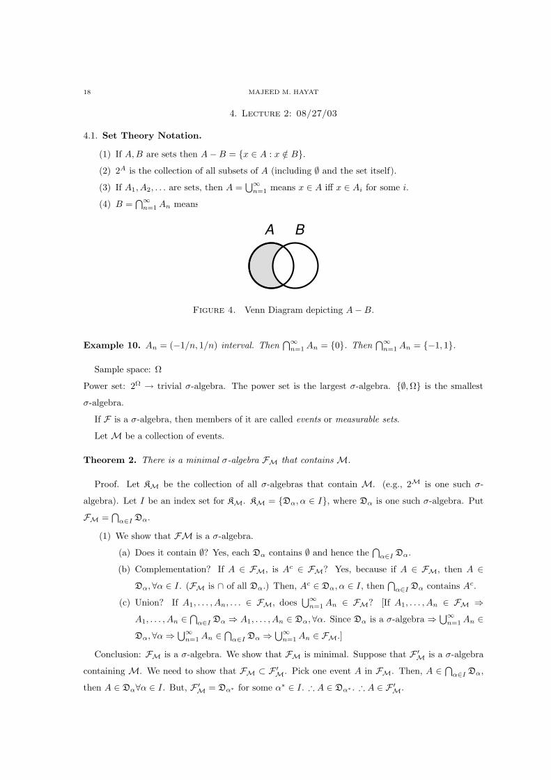
Figure 4. Venn Diagram depicting A − B.

Example 10. An = (−1/n, 1/n) interval. Then⋂∞

n=1 An = 0. Then⋂∞

n=1 An = −1, 1.

Sample space: Ω

Power set: 2Ω → trivial σ-algebra. The power set is the largest σ-algebra. ∅,Ω is the smallest

σ-algebra.

If F is a σ-algebra, then members of it are called events or measurable sets.

Let M be a collection of events.

Theorem 2. There is a minimal σ-algebra FM that contains M.

Proof. Let KM be the collection of all σ-algebras that contain M. (e.g., 2M is one such σ-

algebra). Let I be an index set for KM. KM = Dα, α ∈ I, where Dα is one such σ-algebra. Put

FM =⋂

α∈I Dα.

(1) We show that FM is a σ-algebra.

(a) Does it contain ∅? Yes, each Dα contains ∅ and hence the⋂

α∈I Dα.

(b) Complementation? If A ∈ FM, is Ac ∈ FM? Yes, because if A ∈ FM, then A ∈Dα,∀α ∈ I. (FM is ∩ of all Dα.) Then, Ac ∈ Dα, α ∈ I, then

⋂

α∈I Dα contains Ac.

(c) Union? If A1, . . . , An, . . . ∈ FM, does⋃∞

n=1 An ∈ FM? [If A1, . . . , An ∈ FM ⇒A1, . . . , An ∈ ⋂α∈I Dα ⇒ A1, . . . , An ∈ Dα,∀α. Since Dα is a σ-algebra ⇒ ⋃∞

n=1 An ∈Dα,∀α ⇒ ⋃∞

n=1 An ∈ ⋂α∈I Dα ⇒ ⋃∞n=1 An ∈ FM.]

Conclusion: FM is a σ-algebra. We show that FM is minimal. Suppose that F ′M is a σ-algebra

containing M. We need to show that FM ⊂ F ′M. Pick one event A in FM. Then, A ∈ ⋂α∈I Dα,

then A ∈ Dα∀α ∈ I. But, F ′M = Dα∗ for some α∗ ∈ I. ∴ A ∈ Dα∗ . ∴ A ∈ F ′

M.

ECE 541 19

Example 11. Ω = (−∞,∞). A1 = (−∞, 1);A2 = (0,∞). Let M = A1, A2. In this case,

FM = ∅, (−∞,∞), (−∞, 1), (0,∞), (0, 1),−∞, 0], [1,∞), (−∞, 0] ∪ [1,∞).

0 1 ∞-∞Figure 5. .

Remark: If A,B ∈ F then A − B and B − A ∈ F (idea: A − B = A ∩ Bc).

Example 12. U is the collection of all open sets in <. [Reminder: U is open if for every x ∈ U, we

can find ε > 0, so that (x− ε, x + ε) ∈ U] The theorem tells us that there is a minimal σ-algebra that

contains U. This is called a Borel σ-algebra, and includes all the open sets. B contains all open and

closed sets (because it contains complements). Members of B are called Borel sets.

If U is an open set, then B∩U. This means that the collection of all Borel sets each one intersected

with U. This is called the restriction of B to U.

Exercise 1. B ∩ U is a σ-algebra.

4.2. Random Variables. Suppose that Ω, we also have F . We can define a function X on Ω

(really, we have X(ω), ω ∈ Ω) taking values in <. Recall the dart example:

Let D = (x, y) ∈ <2 : x2 +y2 ≤ 1. Ω = “miss”∪D. Let F be the σ-algebra. Define the function

X(ω) by the rule:

(2) X(ω) =

10, if ω = “miss”

√

x2 + y2, if ω ∈ D

Let’s consider the collection of outcomes that correspond to x < 1/2. We write the above event as

ω ∈ Ω : X(ω) < 1/2 = A1 = X−1((−∞, 1/2)), which is the inverse image in Ω of the outcome.

A1 = (x, y) ∈ <2 : x2 + y2 < 1/4 ∈ FA2 = X−1((−∞, 2)) = D ∈ FA3 = X−1((−∞, 11)) = D ∪ “miss” = Ω ∈ FA0 = X−1((−∞, 0]) = ∅ ∈ F

Formal Definition of a Random Variable: Given Ω,F , a mapping x : Ω → < is called a random

variable (r.v.) if X−1((−∞, r)) ∈ F ,∀r ∈ <.

Names:

(1) (Ω,F) is called a measurable space.

20 MAJEED M. HAYAT

(2) Such a mapping is also called a F-measurable transformation.

Back to dart example:

(3) X1(ω) =

1, if ω ∈ D

0, if ω = “miss”

(4) X2(ω) =

2, if ω ∈ (x, y) : x2 + y2 ≤ 1/4

1, if ω ∈ (x, y) : 1/4 < x2 + y2 ≤ 1

0, if ω = “miss”

12

0

Figure 6.

→ X−11 ((−∞, 0]) = ∅

→ X−11 ((−∞, ε)) = “miss”, ε ≤ 1

→ X−11 ((−∞, 0.1)) = “miss”

→ X−11 ((−∞, 1.1)) = “miss” ∪ D = Ω

→ X−11 ((−∞, 1 + ε)) = Ω, ε > 0

Let’s form a σ-algebra from the collection ∅, “miss”,Ω ≡ M1. FM1= ∅, “miss”,Ω,D.

FM1conveys all the information that x conveys about the experiment. We write σ(x) in place of

FM1to emphasize the σ-algebra (or information) that is generated by the r.v. x.

Exercise 2. Find σ(X2).

ECE 541 21

5. Lecture 3: 09/03/2003

5.1. Random Variables. x : Ω → < is called a r.v. if x is F-measurable. Meaning: X−1((−∞, r)) ∈F ,∀r. X−1((−∞, r)) is the inverse image/transformation of (−∞, r) under x.

The σ-algebra generated by the r.v. x is σ(x) = the smallest σ-algebra that contains all the

inverse images of the form X−1((−∞, r))∀r ∈ <.

x

(-∞,r)X-1(-∞,r)

Figure 7.

Let MX = X−1((−∞, r)), r ∈ <. Because X is a r.v., for each r, X−1((−∞, r)) ∈ F , MX is a

collection of events.

∴ By the theorem, there exists a σ-algebra FMXthat minimally contains MX (we call it σ(x)). In

general, σ(x) ⊂ F , but not necessarily equal to F . Thus, by observing the value of the r.v., we may

not be able to answer all the questions embedded in F . (Think of a “miss” or “hit” type r.v. for

the dart example.)

5.2. Properties of Random Variables. The following statements are equivalent:

(1) x is a r.v.

(2) X−1((−∞, r]) ∈ F ,∀r.

(3) X−1((r,∞)) ∈ F ,∀r.

(4) X−1([r,∞)) ∈ F ,∀r.

(5) X−1((a, b)) ∈ F ,∀a, b. [(a, b), (a, b], [a, b), [a, b]]

(6) XB ∈ F ,∀B ∈ B.

Property 6 is the most powerful because (−∞, r), (−∞, r], (r,∞), [r,∞], (a, b), (a, b], [a, b), [a, b]

are Borel sets.

22 MAJEED M. HAYAT

5.3. Measure. A set function P : F → [0, 1] is called a probability measure (or just probability) if:

(1) P (Ω) = 1.

(2) If A1, A2, A3 are mutually disjoint (meaning Ai ∩ Aj = ∅ if i 6= j), then P (⋃∞

n=1 An) =∑∞

n=1 P (An).

Properties of P:

(1) P (∅) = 0;Ω = Ω ∪ ∅. Note: Ω and ∅ are disjoint.

P (Ω) = P (Ω ∪ ∅)1 = P (Ω) + P (∅) = 1 + P (∅)⇒ P (∅) = 0.

(2) If A ∪ B ∈ F , then P (B) ≥ P (A).

B = A ∪ B\A (disjoint).

P (B) = P (A ∪ B\A) = P (A) + P (B\A) ≥ P (A)

A

B

Figure 8.

(3) If A1 ⊂ A2 ⊂ A3 ⊂ A4 . . ., then P (⋃∞

n=1 An) = limn→∞ P (An). f(x) is continuous at xo if

limn→∞ f(xn) = f(xo) if xn → xo as n → ∞.

A3A2A1

Figure 9.

Proof: Put B1 = A1, B2 = A2\A1, . . . , Bn = An\An−1. Now,⋃n

i=1 Bi =⋃n

i=1 Ai = An.

Also,

(5)∞⋃

i=1

Bi =∞⋃

i=1

Ai.

Bi’s are disjoint.

∴ P (⋃∞

i=1 P (Bi) =∑n

i=1 P (Bi) = P (An), true for any n. From Eq. (6),∑n

i=1 P (Bi) is

convergent because it is increasing and the limit is∑∞

n=1 P (Bn).

ECE 541 23

∴ limn→∞ P (An) =∑∞

i=1 P (Bn), but∑∞

i=1 P (Bn) = P (⋃∞

n=1 An).

∴ limn→∞ P (An) = P (⋃∞

n=1 An).

(4) If A1, . . . , An are disjoint, then P (⋃n

i=1 An) =∑n

i=1 P (An).

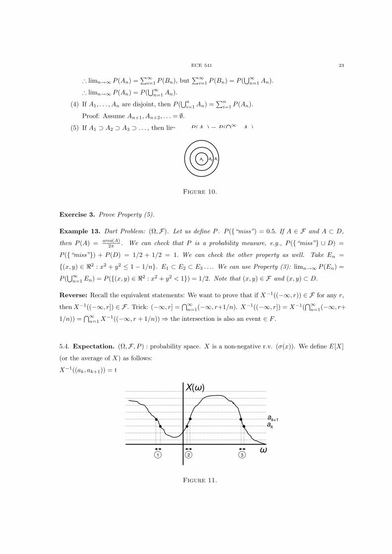
Proof: Assume An+1, An+2, . . . = ∅.(5) If A1 ⊃ A2 ⊃ A3 ⊃ . . . , then limn→∞ P (An) = P (

⋂∞n=1 An).

A1A2A3

Figure 10.

Exercise 3. Prove Property (5).

Example 13. Dart Problem: (Ω,F). Let us define P . P (“miss”) = 0.5. If A ∈ F and A ⊂ D,

then P (A) = area(A)2π . We can check that P is a probability measure, e.g., P (“miss” ∪ D) =

P (“miss”) + P (D) = 1/2 + 1/2 = 1. We can check the other property as well. Take En =

(x, y) ∈ <2 : x2 + y2 ≤ 1 − 1/n. E1 ⊂ E2 ⊂ E3 . . .. We can use Property (3): limn→∞ P (En) =

P (⋃∞

n=1 En) = P ((x, y) ∈ <2 : x2 + y2 < 1) = 1/2. Note that (x, y) ∈ F and (x, y) ⊂ D.

Reverse: Recall the equivalent statements: We want to prove that if X−1((−∞, r)) ∈ F for any r,

then X−1((−∞, r]) ∈ F . Trick: (−∞, r] =⋂∞

n=1(−∞, r+1/n). X−1((−∞, r]) = X−1(⋂∞

n=1(−∞, r+

1/n)) =⋂∞

n=1 X−1((−∞, r + 1/n)) ⇒ the intersection is also an event ∈ F .

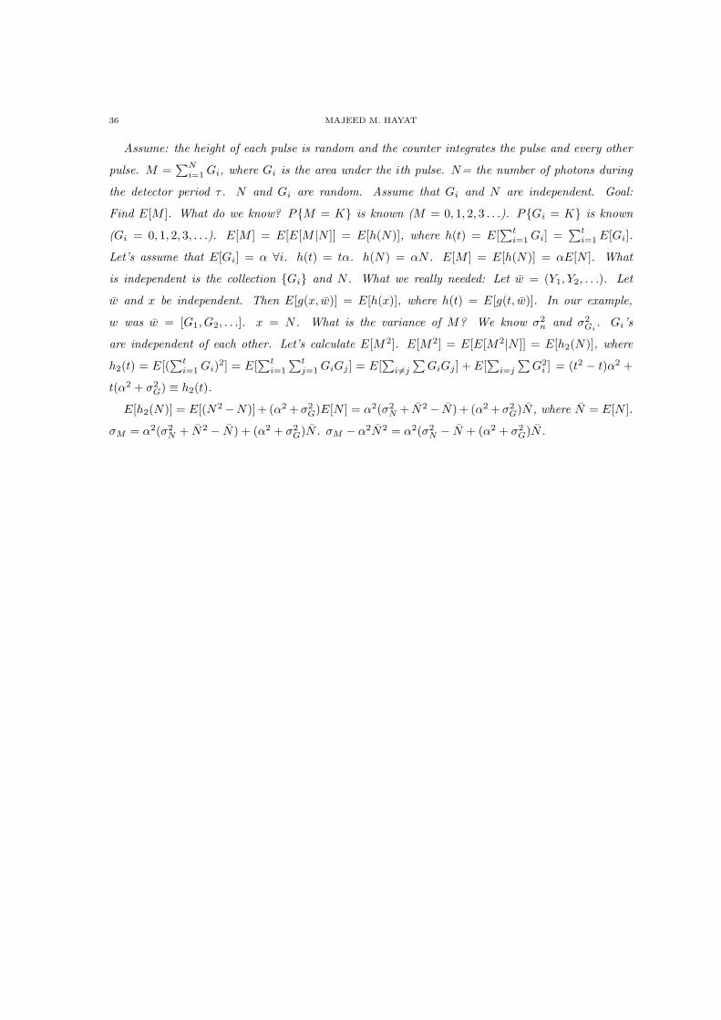
5.4. Expectation. (Ω,F , P ) : probability space. X is a non-negative r.v. (σ(x)). We define E[X]

(or the average of X) as follows:

X−1((ak, ak+1)) = the union of 3 segments ∈ F .

ak

ak+1

1 2 3

X(ω)

ω

Figure 11.

24 MAJEED M. HAYAT

6. Lecture 4: 09/08/2003

6.1. Expectation. (Ω,F , P ): probability space (measure space). Random variable: X : Ω → [0, 1]

and X is F-measurable. In particular, X−1((−∞, r]) ∈ F . Suppose that x ≥ 0.

ω

2-n

Figure 12.

Let’s form (for each n = 1, 2, . . .) Sn =∑∞

i=1i

2n P (ω ∈ Ωi

2n < X(ω) ≤ i+12n ).

ω ∈ Ω : a < X(ω) ≤ b is an event = X−1((a, b]) = X−1((−∞, b])\X−1((−∞, a]) ⇒ difference is

an event. We will show that S1 ≤ S2 ≤ S3 ≤ . . .. In which case, Sn is either convergent or Sn ∞.

We define E[X] = limn→∞ Sn: the expectation of x with respect to probability P . If E[X] < ∞,

then we say that X is integrable. Otherwise, X is not integrable.

Now, suppose that X is arbitrary. Then, we can always write: X = X+ − X−, where X+ =

max(X, 0) and X− = max(−X, 0). Note that both X+ and X− are non-negative r.v.’s. ∴ The

previous expectation stuff applies. In particular, we say X is integrable if E[X+] < ∞ and E[X−] <

∞. In this case, we write E[X] = E[X+] − E[X−].

X

ω

X+ X-

Figure 13.

Show that Sn . Sn =∑∞

i=1i

2n P i2n < x ≤ i+1

2n =∑∞

i=12i

2n+1 P 2i2n+1 < x ≤ 2i+2

2n+1 .Now, ~ = P 2i

2n+1 < x ≤ 2i+22n+1 + P 2i

2n+1 < x ≤ 2i+22n+1 .

∴ Sn =∑∞

i=12i

2n+1 (a2i,n+1 + a2i+1,n+1)

ECE 541 25

=∑∞

i=12i

2n+1 a2i,n+1 +∑∞

i=12i

2n+1 a2i+1,n+1)

≤∑∞i=1

2i2n+1 a2i,n+1 +

∑∞i=1

2i+12n+1 a2i+1,n+1)

≤∑∞j=1 aj,n+1 = Sn+1

∴ limn→∞ Sn makes sense.

Remark: E[|X|] = E[X+] + E[X−].

6.2. Distributions. (Ω,F , P ); x is a r.v. We define the set function µx : B → [0, 1] by the rule:

µx(B) = Px ∈ B = P (X−1(B)), B ∈ B.

F∈A

Ω

B∈B

ℜ

x

Figure 14.

Since x is a r.v., X−1(B) ∈ F . µx is called the distribution induced by x.

Exercise 4. Show that µx is a probability measure on B (Borel set). Check that < is in it: µx(<) =

1. µx(<) = P (X−1(<)) = P (Ω) = 1. Check µx(⋃∞

n=1 Bn) =∑∞

n=1 µx(Bn) if Bi ∩ Bj = ∅, i 6= j.

Hint: Establish the connection between X−1(⋃∞

n=1 Bn) and⋃∞

n=1 X−1(Bn).

6.3. Distribution Function. X is a r.v. We need to find the distribution function Fx(·) as (func-

tion of real variable x) Fx(x) = µx((−∞, x]) = P−∞ < x ≤ x.

Properties of Fx:

(1) Non-decreasing.

(2) limx→∞ Fx(x) = 1, limx→−∞ Fx(x) = 0.

Proof:⋃∞

n=1−∞ < x ≤ n = Ω. P (⋃∞

n=1−∞ < x ≤ n) = P (Ω) = 1. Left hand side

is: limn→∞ P (−∞ < x ≤ n) = limn→∞ Fx(n). We proved: limn→∞ Fx(n) = 1.

Exercise 5. Show that limn→∞ Fx(−n) = 0. Hint: Use the result of HW#2.

26 MAJEED M. HAYAT

6.4. Density Functions. If Fx(·) is differentiable, i.e., dFx(x)dx = fx(x), then E[X] =

∫∞−∞ xfx(x)dx.

Why? E[X] = limn→∞ Sn = limn→∞∑∞

i=1i

2n (Fx( i+12n ) − Fx( i

2n )) ≈ limn→∞∑∞

i=1i

2n fx( i2n )2−n.

But 12n

∑∞i=1

i2n fx( i

2n ) converges to the Riemann Integral:∫∞0

xfx(x)dx. Notation: We write

E[X] =∫

X(ω)dP (ω)(=∫

xdP =∫

xP (dω)).

Also, Sn =∑∞

i=1i

2n P ( i2n < x ≤ i+1

2n ) =∑∞

i=1i

2n µx(( i2n , i+1

2n ]). ∴ We can write E[X] =∫

xdµx(x)(=∫

xµx(dx) : Lebesgue Integral of x w.r.t. µx.∫

xdP : Lebesgue Integral of x w.r.t.

P .

(Ω,F , P ). x is a r.v. E[g(x)] = limn→∞∑∞

i=1 g( i2n )ai,n. If E[X2] < ∞, we say that x is square

integrable.

ECE 541 27

7. Lecture 5: 09/10/2003

7.1. Elementary Hilbert Space Theory. A complex vector space H is called an inner product

space if ∀x, y ∈ H, we have a scaler < x, y > so-called “inner product” such as the following rules

are satisfied:

(1) < x, y >=< x, y >∈ D,∀x, y ∈ H

(2) < x + y, z >=< x, z > + < y, z >,∀x, y, z ∈ H

(3) < αx, y >= α < x, y >,∀x, y ∈ H,α ∈ D

< x,αy >= α < x, y >

(4) < x, x >≥ 0,∀x ∈ H

< x, x >= 0 iff x = 0

7.2. Schwarz Inequality. Properties Rules (1)-(4) imply that: | < x, y > | ≤ ||x|| ||y||,∀x, y ∈ H

Proof: Assume A = ||x||2 and C = ||y||2 and B = | < x, y > |. < x − αry, x − αry >≥ 0, r ∈<, α ∈ D. < x, x − αry > − < rαy, x − αry >≥ 0. ~ = ||x2|| − rα < y, x > −rα < x, y >

+r2||y2|| ≥ 0,∀r ∈ < and ∀α ∈ D. Choose: α : α < y, x >= | < x, y > |. Note that α = <x,y>|<x,y>|

and |α| = |<x,y>||<x,y>| = 1. ~ ⇒ ||x2|| − 2r| < x, y > | + r2||y2|| ≥ 0 → A − 2rB + r2C ≥ 0, r ∈ <.

r1,2 = 2B±√

4B2−4AC2C = B±

√B2−ACC . B2 − AC ≥ 0. B2 ≥ AC ⇒ | < x, y > |2 ≤ ||x||2||y||2 ⇒ | <

x, y > | ≥ ||x|| ||y||.

rr1 r2

Figure 15.

7.3. Triangle Inequality. It follows from Schwarz Inequality: ||x + y|| ≤ ||x||+ ||y||,∀x, y ∈ H. It

follows from the Triangle Inequality that: ||x − z|| ≤ ||x − y|| + ||y − z||. If we look at the distance

between the two vectors x, y ∈ H as: d(x, y) = ||x − y||, then we define H with the metric d as a

metric space (H, d). d : H × H → <+. Now, if H is complete, then H is called a Hilbert Space.

Complete space H means any Cauchy sequence in H converges to a point that lies in H. Cauchy

sequence: yn∞n=1 is called a Cauchy sequence if for any ε > 0,∃ a large number N such that

||yn − ym|| ≤ ε for n,m > N .

Exercise 6. Prove the Triangle Inequality. Hint: < x + y, x + y >= . . ..

28 MAJEED M. HAYAT

7.4. Convex Sets. A set E in a vector space V is said to be a convex set if for any x, y ∈ E, and

t ∈ (0, 1), the following point Zt = tx + (1 − t)y ∈ E. In other words, the line segment between x

and y lies in E. E + x = y + x : y ∈ E is a convex set.

7.5. Orthogonality. If < x, y >= 0, then we say that x and y are orthogonal. We write x ⊥ y. ⊥is a symmetric relation: x ⊥ y ⇔ y ⊥ x.

Pick a vector x ∈ H, then find all vectors in H that are orthogonal to x. We write it as:

x⊥ = y ∈ H :< x, y >= 0 and x⊥ is a closed subspace.

Let M be a subspace in H (M ⊂ H). Define M⊥. M⊥ =⋂

x∈M x⊥,∀x ∈ M.

Theorem 3. Any non-empty, closed an convex set E ⊂ H contains a unique element with smallest

norm. ∃xo ∈ E : ||xo|| < ||x||, x ∈ E.

Proof: “Parallelogram Law”. ||x + y||2 + ||x − y||2 = 2||x||2 + 2||y||2,∀x, y ∈ H. Let δ = inf||x|| :

x ∈ E.

x+y

x-y

Figure 16.

Uniqueness: Replace x by x/2 and y by y/2. In the parallelogram law: ||x/2 + y/2||2 − ||x/2 −y/2||2 = 1

2 ||x||2 + 12 ||y||2. ||x−y||2 = 2||x||2 +2||y||2−4||x+y

2 ||2. Assume that x+y2 ∈ E (E is convex).

||x+y2 ||2 = δ2.

(6) ||x − y||2 = 2||x||2 + 2||y2|| − 4δ2.

Assume ||x|| = |y|| = δ. Substitute in Eq. (6) ⇒ ||x − y||2 = 2δ2 + 2δ2 − 4δ2 = 0 ⇒ x = y ⇒ there

is a unique element.

Existence: Assume yn∞n=1 such that limn→∞ ||yn|| = δ. ||x − y||2 = 2||x||2 + 2||y||2 − 4δ2.

Replace x by yn and y by ym. Then ||yn −ym||2 = 2||yn||2 +2||ym||2 −4δ2. limn,m→∞ ||yn −ym||2 =

2 limn→∞ ||yn||2 + 2 limm→∞ ||ym||2 − 4δ2 ⇒ limn,m→∞ ||yn − ym||2 = 2δ2 + 2δ2 − 4δ2 = 0. So,

yn∞n=1 is a Cauchy sequence. Since H is complete then ∃xo ∈ H : yn → xo.

Example 14. For any fixed n, the set Dn of all n-tuples x = (x1, x2, . . . , xn), xi ∈ D is a Hilbert

Space, where < x, y >=∑n

i=1 xiyi, Y = (y1, y2, . . . , yn).

Example 15. L2[a, b] = f(x) :∫ b

a|f(x)|2dx < ∞, x ∈ [a, b] is a Hilbert Space, where < f, g >=

∫ b

af(x)g(x)dx. ||f || =

√< f, f > = [

∫ b

a|f |2dx]1/2 = ||f ||2.

ECE 541 29

8. Lecture 6: 09/15/03

Exercise 7. Show that the Schwarz Inequality is an equality if y = αx. α ∈ D, i.e., | < x,αx > | =

||x|| · ||αx||.

8.1. Triangle Inequality. < x + y, x + y >=< x, x > + < y, y > + < x, y > + < y, x >=

||x||2 + ||y||2+ < x, y > + < x, y >∗. But, if c ∈ D, then c+c∗ ≤ 2|c|. ||x+y||2 ≤ ||x||2 + ||y||2 +2| <

x, y > | ≤ ||x||2 + ||y||2 + 2||x|| ||y|| = (||x|| + ||y||)2. ∴ ||x + y|| ≤ ||x|| + ||y||. Equality holds if

< x, y >= 0 (x ⊥ y).

8.2. Notion of a Closed Set. We have a norm, i.e., we say ||x|| is a norm on if:

(1) ||x|| ≥ 0.

(2) ||x|| = 0 only if x = 0.

(3) ||x + y|| ≤ ||x|| + ||y||.(4) ||αx|| = |α| ||x||, α ∈ D.

Exercise 8. Show that ||x|| =< x, x >1/2 is a norm on .

We say xn → x, whenever xn ∈ H and x ∈ H if limn→∞ ||xn−x|| = 0 or ||xn−x|| → 0 as n → ∞.

Suppose that M ⊂ H. We say that M is closed if it happens that xn → x ∈ H, then necessarily

x ∈ M. H is called complete whenever xn, xm have the property that ||xn − xm|| → 0 as m,n tend

to ∞. Then, xn is a convergent sequence, i.e., ∃xo ∈ H for which xn → xo. H is complete if every

Cauchy sequence is convergent.

Fact: If H is complete, then it is closed.

Recall: If M is a closed and convex subset of a Hilbert Space (complete inner-product space), the

M contains a unique element of minimal norm.

2ℜ=H

element ofminimal norm

M

Figure 17. A line is closed. M is convex and closed.

30 MAJEED M. HAYAT

Theorem 4. Projection onto closed subsets. If M ⊂ H,H is in Hilbert Space, M is closed. Then

for every x ∈ H,∃ a decomposition x = Px + Qx, where Px ∈ M, Qx ∈ M⊥ (M⊥ =⋂

y∈Mx ∈H, < x, y >= 0) and

(1) The decomposition is unique.

(2) ||x||2 = ||Px||2 + ||Qx||2.(3) If M 6= H, then ∃ y ∈ H, y /∈ M such that y ⊥ M.

(4) Px is the nearest point in M to x. Qx is the nearest point in M⊥ to x. Px is called the

projection of x into M. Qx is called the projection of x into M⊥.

2ℜ=Hℜ=M

M

Px

Qx

x

Figure 18.

8.3. Application. (Ω,F , P ). Let D ⊂ F (e.g., D could be σ(x) if x is a r.v. defined on (Ω,F).

Let L2(P ) denote all the r.v.’s (F-measurable) that are square integrable, i.e., if x ∈ L2(P ), then

E[|x|2] < ∞.

Claim: L2(P ) is a vector space. Check closure under addition. Suppose X,Y ∈ L2(P ), we need to

check that E[|X + Y |2] < ∞ in which case X + Y ∈ L2(P ). What is an inner product here? We

define < X,Y >= E[XY ] (think of XY as a new variable Z). Also, < x, x >= ||x2|| = E[X2]. We

can check that < X,Y > is an inner product. We need to show that: ||X + Y || < ∞ (finite) ↔E[|X + Y |2]1/2. E[|X + Y |2] = ||X + Y ||2 ≤ ||X||2 + ||Y ||2 ⇒< ∞. Also, let’s do closure under

scalar multiplication. If x ∈ L2(P ), then ||αx|| = E[|αx|2]1/2 = |α|E[|x|2]1/2 = |a| ||x|| < ∞.

Let L2(D) be the collection of all D-measurable square integrable r.v.’s, i.e. if x ∈ L2(D) then,

(1) x is D-measurable.

(2) E[|x|2] < ∞.

Then, L2(D) is also a vector space. Note that L2(D) ⊂ L2(P ) and since L2(D) is itself a vector

space L2(D) is a subspace of L2(P ). We have the following:

(1) L2(P ) is a vector space (its also complete) so its a Hilbert Space.

(2) L2(D) is a closed subspace of L2(P ).

ECE 541 31

Think of L2(P ) as H. Think of L2(D) as M. According to the projection theorem, if x ∈ L2(P ),

then we can write x as X = PX + QX, where PX ∈ M and QX ∈ M⊥. We define E[X|D] , PX.

First, note that E[X|D] is a D-measurable r.v.

Exercise 9. (1) Show that if x is a D-measurable r.v. then so is aX, a ∈ <. (2) Show that if X

and Y are D-measurable, so is X + Y .

Special Case: D = σ(Y ), Y ∈ L2(P ). Then, we can still talk about E[x|σ(Y )]: is a square

integrable σ(Y )-measurable r.v.

Theorem 5. If Z is a σ(Y )-measurable r.v. then we can write Z = h(Y ), where h is a Borel-

measurable function, meaning: h−1(B) ∈ B (or all B ∈ B). E[X|σ(Y )] is a function of Y and we

write it as E[X|Y ].

32 MAJEED M. HAYAT

9. Lecture 7: 09/17/03

Theorem 6. Projection Theorem: H: Hilbert Space. M: Closed subset in H.

(1) Every x ∈ H has a unique decomposition. x = Px + Qx, where Px ∈ M and Qx ∈ M⊥.

(2) Px is the nearest point in M to x. Qx is the nearest point in M⊥ to x.

(3) If we think of Px as mapping x to Px, then P is linear. The same can be said about Qx.

(4) ||x||2 = ||Px||2 + ||Qx||2.Proof: Uniqueness. Suppose that we have x = x′+y′ and x = x′′+y′′. Then, x′+y′ = x′′+y′′,

x′ − x′′ = y′′ − y′. ∴ x′ − x′′ = y′′ − y′ = 0 since the same element ∈ M and ∈ M ⊥.

∴ x′ = x′′, y′ = y′′ → unique.

2ℜ=H

x+M

Shortest distance Qx

Figure 19. Elevating M by x.

2ℜ=H

MPx

Qx

x

Figure 20.

Consider M + x = x + y : y ∈ M. Claim: M + x is closed. M is closed, so, if xn ∈ M and

as n → ∞, xn → xo (||xn − xo|| → 0) then xo → M. Pick a convergent sequence in x + M, call it

Zn. Zn = x + yn, yn ∈ M. Since Zn is convergent, so is yn, but the limit of yn is in M since M is

closed.

ECE 541 33

We show that x + M is convex. Pick x1 and x2 ∈ x + M. We need to show that for any

0 ≤ α ≤ 1, αx1 + (1 − α)x2 ∈ x + M. But x1 = x + y1, y1 ∈ M and x2 = x + y2, y2 ∈ M.

αx1 = αx + αy1 → αx1 + (1 − α)x2 = x + αy1 + (1 − α)y2 →∈ x + M ∈ M (since M is convex).

(1 − α)x2 = (1 − α)x + (1 − α)y2 ∈ x + M. ∴ By the earlier theorem, ∃ a member in x + M of

smallest norm. Call it Qx. Let Px = x−Qx. Note that Px ∈ M. We need to show that Qx ∈ M⊥.

Namely, < Qx, y >= 0, ∀ y ∈ M. Call Qx = z. ||z|| ≤ ||y||, ∀ y ∈ M + x. Pick y = z − αy, where

y ∈ M, ||y|| = 1. ||z||2 ≤ ||z − αy||2 =< z − αy, z − αy >. 0 ≤ −α < y, z > −α < z, y > +||α||2.Pick α =< z, y >. We obtain 0 ≤ −| < z, y > |2. This can hold only if < z, y >= 0, i.e., z is

orthogonal to every y ∈ M. ∴ Qx ∈ M⊥.

9.1. Minimum Distance Properties. Show that Px is the nearest point in M to x. y ∈ M,

||x − y||2 = ||Px + Qx − y||2 = ||Qx + (Px − y)||2 = ||Qx||2 + ||Px − y||2: Pythagoras. ∴ Px is the

member in M which is nearest to x. The Qx case is shown similarly.

9.2. Linearity. Take x, y ∈ H. x = Px+Qx. y = Py +Qy. (ax+ by) = P (ax+ by)+Q(ax+ by) =

aPx + aQx + bPy + bQy. P (ax + by)− aPx− bPy = −Q(ax + by) + aQx + bQy → The only vector

that satisfies the equation is 0. ∴ P (ax + by) = aPx + bPy. Q(ax + by = aQx + bQy.

Comment: If x ∈ M, then Qx = 0 and x = Px. (Ω,F , P ). x is a r.v. D ⊂ F . L2(P ) =

Y : E[Y 2] < ∞. L2(P ) is a vector space. L2(P ) is closed. Why? xn → xo (this means

that E[|xn − xo|]2 → 0 as n → ∞). xn ∈ L2(P ). E[x2o] < ∞. E[x2

o] = E[(xo − xn + xn)2] =

E[(xo − xn)2] + E[x2n] + 2E[xn(xo − xn)] ≤ 2E[x2

n]1/2E[(xn − xo)2]1/2 < ∞. L2(P ) is closed inner

product space: < x, y >= E[XY ]. L2(D) = D-measurable Y : E[Y 2] < ∞. L2(D) is also closed

(same reason). Let M = L2(D) and H = L2(P ). We apply the projection theorem to x ∈ L2(P ).

x = Px + Qx, where Px ∈ L2(D), Qx ∈ L2(D)⊥. We have the property that: ||x − Px|| ≤ ||x − y||∀ y ∈ L2(D). We call Px the conditional expectation of x given D. Px = E[x|D].

9.3. Properties of Conditional Expectation.

(1) Call E[X|D] = Z. E[XY ] = E[ZY ], Y ∈ L2(D). Interpretation: Z contains all the infor-

mation that X contains relevant to Y .

Proof: E[XY ] = E[(PX + QY )Y ] = E[(PX)Y ] + E[(QX)Y ] = E[ZY ]. Conversely, if a

r.v. in L2(D) has the property that E[ZY ] = E[XY ]∀ Y ∈ L2(D) then Z = E[X|D].

Alternative definition of E[X|D]. z = E[X|D] if E[ZY ] = E[XY ]∀ Y ∈ L2(D).

(2) E[a|D] = a. We need to show that E[aY ] = E[aY ].

(3) E[X] = E[E[X|D]]. Z = E[X|D]. E[ZY ] = E[XY ],∀ Y ∈ L2(D), for Y = 1 (note that 1 is

Ω, ∅ measurable, so it is also D-measurable) → E[X] = E[Z].

(4) E[Y |D] = Y if Y ∈ L2(D) (e.g., E[X|X] = X). Check: E[Y ω] = E[Y ω], ω ∈ L2(D).

34 MAJEED M. HAYAT

(5) E[XY |D] = Y E[X|D] if Y ∈ L2(D)(E[XY |Y ] = Y E[X|Y ].

(6) Let D1 ⊂ D2 ⊂ F . E[X|D1] = E[E[X|D2]|D1]. Also, E[X|D1] = E[E[X|D1]|D2]. Take

D = Ω, ∅. Then E[X|D] = E[X]. E[X|D] is D-measurable. ∴ E[X|D] must be a cte if

D = Ω, ∅.

Let D = σ(Y ), Y ∈ L2(P ). Then E[X|D] = Z = h(Y ).

Theorem 7. If Z is D-measurable, then there exists a function h such that Z = h(Y ).

In this case, we write Z = E[X|Y ].

ECE 541 35

10. Lecture 8: 09/22/03

If Z = E[X|D],D ⊂ F , then

(7) E[ZY ] = E[XY ], Y ∈ L2(D).

We use Eq. (7) as the defining property for E[X|Y ]. To be able to do so, we need to show: If Z,

a D-measurable r.v., has the property that E[XY ] = E[ZY ], then Z must be = E[X|D] (= Px).

We need to show that Z = Px. Note that E[XY − ZY ] = 0,∀ Y ∈ L2(D). ∴ E[Y (X − Z)] = 0.

E[Y (PX + QY −Z)] = 0. E[Y PX] + E[Y QX]−E[Y Z] = 0. E[Y (Z −PX)] = 0,∀ Y ∈ L2(D). In

particular, take

(8) Y =

1, if Z − PX ≥ 0

−1, if Z − PX < 0

Claim: Y ∈ L2(D). E[Y (Z − PX)] = E[|Z − PX|] = 0 by the assumption. ∴ Z − PX = 0 → Z =

PX.

Property 9. Smoothing Property: E[X|D1] = E[E[X|D2]|D1]. D1 ⊂ D2 ⊂ F .

Proof: Need to show: E[ZY ] = E[XY ],∀ Y ∈ L2(D1). LHS: E[Y E[E[X|D2]|D1]. Note that

E[E[X|D2]|D1] is D1-measurable = E[E[Y E[X|D2]|D1]]. Note that Y is also D2-measurable (∈L2(D2)) = E[E[E[XY |D2]|D1]]. But, E[E[Y X|D2]] = E[XY ] = E[E[XY ]] = E[XY ].

Property 10. If X and Y are independent r.v.’s, then E[g(x, y)] = E[h(y)], where h(t) = E[g(x, t)].

Special Case: E[XY ] = E[E[XY |Y ]] = E[Y E[X|Y ]]. h(t) = E[tx] = tE[x]. h(Y ) = Y E[X].

E[h(Y )] = E[Y E[X|Y ]]. Omit general proof beyond special case.

Example 16. Photon counting: Energy of photon = hv, where h is Planck’s constant and v is the

wave frequency in Hertz.

radiation

detection

current

……….

N photons

electric pulses

counter M

Figure 21.

36 MAJEED M. HAYAT

Assume: the height of each pulse is random and the counter integrates the pulse and every other

pulse. M =∑N

i=1 Gi, where Gi is the area under the ith pulse. N= the number of photons during

the detector period τ . N and Gi are random. Assume that Gi and N are independent. Goal:

Find E[M ]. What do we know? PM = K is known (M = 0, 1, 2, 3 . . .). PGi = K is known

(Gi = 0, 1, 2, 3, . . .). E[M ] = E[E[M |N ]] = E[h(N)], where h(t) = E[∑t

i=1 Gi] =∑t

i=1 E[Gi].

Let’s assume that E[Gi] = α ∀i. h(t) = tα. h(N) = αN . E[M ] = E[h(N)] = αE[N ]. What

is independent is the collection Gi and N . What we really needed: Let w = (Y1, Y2, . . .). Let

w and x be independent. Then E[g(x, w)] = E[h(x)], where h(t) = E[g(t, w)]. In our example,

w was w = [G1, G2, . . .]. x = N . What is the variance of M? We know σ2n and σ2

Gi. Gi’s

are independent of each other. Let’s calculate E[M 2]. E[M2] = E[E[M2|N ]] = E[h2(N)], where

h2(t) = E[(∑t

i=1 Gi)2] = E[

∑ti=1

∑tj=1 GiGj ] = E[

∑

i6=j

∑

GiGj ] + E[∑

i=j

∑

G2i ] = (t2 − t)α2 +

t(α2 + σ2G) ≡ h2(t).

E[h2(N)] = E[(N2 −N)] + (α2 + σ2G)E[N ] = α2(σ2

N + N2 − N) + (α2 + σ2G)N , where N = E[N ].

σM = α2(σ2N + N2 − N) + (α2 + σ2

G)N . σM − α2N2 = α2(σ2N − N + (α2 + σ2

G)N .

ECE 541 37

11. Lecture 9: 09/29/03

11.1. Applications of Conditional Expectations: Problem: We flip a H-T coin successively.

Suppose PH = p and PT = q = 1 − p. Coin flips are independent of each other. Y1 = mini ≥1 : x1, . . . , xi−1 = 0, xi = 1, where

(9) xi =

1, ith flip is a “H”

0, ith flip is a “T”

xi’s are independent of each other. Y1 is the flip index at which we see a head for the first time.

E[Y1] . . ..

NOTE: THIS IS AN INTENTIONALLY SHORT LECTURE.

38 MAJEED M. HAYAT

12. Lecture 10: 10/01/03

Experiment: Toss a coin repeatedly, infinitely many times and observe a sequence of heads and

tails. Random variables: We define Tn, n = 1, 2, 3, . . . ;ω = (ω1, ω2, . . .).

(10) Tn =

1, ωn = H

0, ωn = T

Y1 = mini : xi = 1. More generally, Yk = mini : Ti = Ti+1 = . . . = Ti+k−1 = 1 for each Yk, Yk

is a r.v. on Ω = (ω1, ω2, . . .) : ωi ∈ H,T. Yk = E[Yk].

Special case: k = 1, Range Y1? R(Y1) = 1, 2, 3, 4, . . .. Assume PH = p and q = 1− p (P (T )).

Then, assuming coins are independently flipped:

PY1 = 1 = p.

PY1 = 2 = qp.

PY1 = 3 = q2p...

PY1 = n = qn−1p → p∑∞

i=1 qi−1 = pq (−1 + 1

1−q ) = pq ( 1

p − 1) = 1. y1 =∑∞

i=1 iPY1 = i =∑∞

i=1 ipqi−1 = pq

∑∞i=1 iqi.

Define g(q) =∑∞

i=1 qi = (−1 + 11−q ) = (−1 + 1

p ) = −1 + 11−q . g′(q) =

∑∞i=1 iqi−1 = 1

q

∑∞i=1 iqi.

g′(q) = 1(1−q)2 → 1

(1−q)2 = 1q

∑∞i=1 iqi →∑∞

i=1 iqi = q(1−q)2 = 1−p

p2 . ∴ y1 = pq

qp2 = 1

p for p = 12 ; y1 =

2.

Claim: Yk = h(Yk−1, T (Yk−1+k−1), T (Yk−1+k), . . .). Note that Yk−1 and TYk−1+k−1, TYk−1+k, . . .are independent. ∴ E[Yk] = E[h(Yk−1, T (Yk−1 + k − 1), T (Yk−1 + k), . . .)] = E[g(Yk−1)], where

g(t) = E[h(t, TYk−1+k−1, . . .)].

Now, we fix Yk−1 = t. Consider E[h(t, Tt+k−1, Tt+k, . . .)]. Notation: A ∈ F . We define IA(ω), a

r.v., as follows:

(11) IA(ω) =

1, ω ∈ A

0, ω /∈ A

which we call the indicator function for the event A. Let A = Tt+k−1 = 1. E[h(t, Tt+k−1, . . .)|Tt+k−1] =

tIA + (t + (k − 1) + yk)IcA (IA is random). ∴ E[h(t, Tt+k−1, . . .)] = E[E[h(t, Tt+k−1, . . .)|Tt+k−1]] =

E[tIA + (t + (k − 1) + yk)IcA =tp(A) + (t + (k − 1) + yk)p(Ac) = tp + (t + (k − 1) + yn)q.

yk = E[g(Yk−1)] = E[Yk−1p + (Yk−1 + k − 1 + yk)q = pyk−1 + q(yk + k − 1) + qyk−1.

(12) yk = p−1yk−1 +q

p(k − 1).

y1 = 1p . If p = 1

2 , then y2 = 2y1 + 1 = 5. General Solution: yk = ( 1p−1 + 1 + p2

q )( 1p

k − k − pq .

ECE 541 39

Example 17. Example of Property (7) of E[X|Y ]. In E[h(X,Y )] = E[g(Y )], where g(t) =

E[h(x, t)] if X and Y are independent.

Example 18. Counter-example. Let Y = XZ where Z = 1 + X. Now, E[Y ] = E[XZ] = E[X(1 +

X)] = x+x2. By property (7), z = t, E[XZ] = E[X]t. E[E[X]Z] = E[X]E[Z] = E[X](1+E[X]) =

x + x2. Note that the two are different, i.e., x2 6= x2.

40 MAJEED M. HAYAT

13. Lecture 11: 10/06/03

13.1. Independence. (Ω,F , P ). D1 ⊂ D2 ⊂ F . We say D1 and D2 are independent sub-σ-algebras

if PA ∩ B = PAPB∀A ∈ D1, B ∈ D2. If x is D1-measurable, Y is D2-measurable, we say

that X and Y are independent. Naturally, if X and Y are independent, then PX ∈ A, Y ∈ B for

A,B ∈ B (=P (x ∈ A ∩ PY ∈ B) = Px ∈ APY ∈ B).Special Case: Take D1 = σ(x) and D2 = σ(y). X and Y are independent if σ(x) and σ(y) are

independent. Claim: µx,y(A,B) = µx(A)µy(B),∀A,B ∈ B, where µx,y(A,B) = Px ∈ A, y ∈ B.The proof is clear.

µx,y is called the joint distribution of the r.v.’s X and Y . If X and Y are independent, then

Fxy(x, y) = Fx(x)Fy(y). If X and Y have densities, then the joint pdf of X and Y also factors if X

and Y are independent. fxy(x, y) = fx(x)fy(y). [µxy(A,B) = PX ∈ A, Y ∈ B. If A and B are in

<, consider A × B: µxy(A,B) = P(x, y) ∈ A × B.In general, as a function of A, µxy(A,B) is a measure on B. As a function of B, µxy(A,B) is a

measure on B. If A = (−infty, x] and B = (−∞, y], then µxy((−∞, x], (∞, y]) = PX ≤ x, Y ≤y = Fxy(x, y).

a b

y

xix∆

iy∆

Figure 22.

∑

f(xi)δxi →∫ b

af(t)dt (Riemann) = limδyi→0

∑

yiµ(yi < y ≤ yi+1) =∫ b

af(t)dµ (Lebesgue

measure on <).

not integrable

x1

Figure 23. The inverse of this function looks like 1x2 → it is integrable (finite)

but cannot be used in the Riemann Integral.

ECE 541 41

13.2. Parameter Estimation. Suppose that x is a r.v. It has a pdf fx(·); fx(·) is parameterized

by a parameter θ ∈ Θ.

Example 19. x is a Gaussian with mean θ and variance 1. fx(x) = 1√2πσ2

e−(x−θ)2/2σ2

, Θ is

arbitrary.

0

1

t

received signal

1=θ0=θ

1,0=Θ0

1

Figure 24.

Let x1, x2, x3, . . . , xn be independent samples (realizations) of x. A function Θn defined on

x1, . . . , xn is called an estimator of the parameter θ if the range of Θn is in Θ.

Recall fx(x) ∼ N(θ, 1). To extract θ, we can do:

(1) Threshold test.

(2) 1n

∑ni=1 xi: the fluctuations average to 0.

(3) Plug x1, . . . , xn into fx1(·)fx2

(·) . . . fxn(·) (look at the likelihood of the parameters) → Max-

imum Likelihood Estimation (MLE).

(4) Find θn(x1 . . . xn) for which the mean square error is minimized, i.e., E[|θn(x1 . . . xn)− θ|2]is minimal → Minimum-Mean-Square Error estimators (MMSE).

(5) Linear Estimator: As in 4), but we restrict θn to be linear in data. θn(x1 . . . xn) = a1x1 +

a2x2 + . . .+anxn = aT xn. Let’s try 1n

∑ni=1 xi = θn: x ∼ N(0, 1). Assume that Θ = <. We

want low variability in θn from xn to xn.

)(inx

)(ˆ inθ

better

Figure 25. We want a small “offset”.

42 MAJEED M. HAYAT

The bias of an estimator θn is b(θn) = E[θn] − θ. The variability of an estimator θn is captured

by the variance of θn: var(θn).

For now, let’s consider: P| 1n∑n

i=1 xi−θ| > ε. Assume that b(θn) = 0 (no offset). E[ 1n

∑ni=1 xi] =

1n

∑ni=1 E[xi] = 1

n

∑ni=1 θ = nθ

n = θ → Assumption is correct. Put Y = 1n

∑ni=1 xi, E[Y ] = Y .

P|Y −Y | > ε = E[I|Y −Y |>ε(ω)·1] ≤ E[I|Y −Y |>ε(ω)( |Y −Y |ε )2] ≤ E[( |Y −Y |

ε )2] = 1ε2 E[|Y −Y |2] =

1ε2 σ2

Y .

In our case, Y = 1n

∑ni=1 xi. σ2

Y = 1n . ∴ P| 1n

∑ni=1 xi − θ| > ε ≤ 1

ε21n . For any ε > 0, if we

make n large enough we can drive the above probability to zero.

ECE 541 43

14. Lecture 12: 10/13/03

14.1. Parameter Estimation. Model: x1x2x3 . . . xn. xi’s are iid. x1 ∼ N(θ, σ2), θ ∈ Θ. Goal:

Find a function on (x1, x2, . . . , xn) that maps the data to the parameter space Θ. Proposal: Θn =

1n

∑ni=1 xi.

n

tn1

n2

)(tfn

Figure 26.

For any t, the limit converges to 0. limn→∞ fn(t) = 0,∀t.∫∞0

fn(t)dt = 1. ∴ limn→∞∫∞0

fn(t)dt 6=∫∞0

limn→∞ fn(t)dt = 0.

14.2. Chebychev’s Inequality. P|x − E[X]| > ε ≤ var(x)ε2 . P|x − E[X]| > ε ≤ E[φ|x−E[X]|]

φ(ε)

General form: If φ is an increasing function on [0,∞), then Pφ(|x − E[X]|) > ε ≤ 1φ(ε)E[φ(|x −

E[X]|)]. In particular, if φ(t) = t2 then we have P(x − E[X]) > ε ≤ var(x)ε2 . (key step in proof)

|x − E[X]| > ε = φ(|x − E[X]|) > φ(ε) and 1 ≥ Iφ(|x−E[X]|)>ε(ω). Back to Θn = 1n

∑ni=1 xi.

E[Θn] = θ. By Chebychev, P|Θn − θ| > ε ≤ textvar(Θn)ε2 . Fact (check): var(Θn) = 1

nσ2. ∴

P|Θn − θ| > ε ≤ σ2

nε2 , i.e., for any ε > 0, we can find no such that P|Θno− θ| > ε ≤ δ, where δ

is arbitrarily small. pn ≤ σ2

nε2 . Claim: limn→∞ pn = 0.

Definition 6. If pn is a sequence, we define the limit superior of pn as limn→∞ supk≥n pk exists.

We call it limn→∞ pn.

k

n1

n

Figure 27.

Limit inferior: limn→∞ infk≥n pk (non-decreasing). ∴ limn→∞ infk≥n pk exists. We call it limn→∞ pn.

44 MAJEED M. HAYAT

We say limn→∞ pn exists if limn→∞ pn = limn→∞ pn (we call it limn→∞ pn).

Fact: In general lim pn ≤ lim pn. In our case, limn→∞ pn ≤ limn→∞σ2

nε2 = limn→∞σ2

nε2 = 0.

0 ≤ limn→∞ pn ≤ limn→∞ pn ≤ 0. ∴ limn→∞ pn = limn→∞ pn = limn→∞ pn = 0. Conclusion:

limn→∞ P|θn − θ| > ε = 0. We say that the estimator θn converges in probability to 0.

14.3. Weak Law of Large Numbers. If x1, x2, x3, . . . , xn are iid and E[|x1|] < ∞. Assume

var(x1) < ∞. Then if we form zn = 1n

∑ni=1 xi, then zn converges to E[x1] in probability.

Proof: P|zn − E[zn]| > ε = P|zn − E[x1]| > ε ≤ var(zn)ε2 = 1

nvar(x1)

ε2 → 0.

Moreover: If E[x1] = ∞, then we can prove that zn → ∞ in probability. limn→∞ Pzn > m = 1.

14.4. Maximum Likelihood Estimation. x1, x2, . . . , xn. Suppose we have a joint pdf: fx1,...,xn(x1, . . . , xn).

Suppose that the joint pdf involves an unknown parameter θ ∈ Θ. Given that the data x1, . . . , xn

is available, we look at fx1,...,xn(x1, . . . , xn) and find θo ∈ Θ that maximizes it. We call such θo the

maximum likelihood estimate of θ.

Example 20. x1, . . . , xn, x1 ∼ N(θ, 1) and are iid. fx1,...,xn(x1, . . . , xn) =

∏ni=1 fx1

(xi) =∏n

i=11√2π

e−(xi−θ)2

2 =

1

(2π)n2

e−nθ2

2

∏ni=1 e(θxi−

x2i2 ). Assume Θ = (−∞,∞). We look at fx1,...,xn

(x1, . . . , xn) and maximize

it over θ.

Let’s maximize it:

(2π)n2

ddθ fx1,...,xn

(x1, . . . , xn) = −θne−nθ2

2

∏ni=1 eθxi−

x2i2 +e

−nΘ2

2 (∏n

i=1 e−x2

i2 )(∑n

i=1 xi)eθ∑n

i=1 xi =

0. ∴ 0 = −θne−nθ2

2 eθ∑n

i=1 xi + e−nθ2

2 (∑n

i=1 xi)eθ∑n

i=1 xi . θo = 1n

∑ni=1 xi. (Do a second derivative

check). ∴ θo = 1n

∑ni=1 xi.

Example 21. Suppose that xi has the following pdf:

(13) fxi(x) =

1a , 0 ≤ x ≤ a

0 otherwise

a1

)(xfix

a x

Figure 28.

a is unknown. aMLE = max(x1 . . . xn) to get as close as possible to a.

ECE 541 45

15. Lecture 13: 10/15/03

15.1. Maximum Likelihood Estimation. If x1 ∼ N(θ, 1), then θML = 1n

∑ni=1 xi. Suppose

x1, . . . , xn are iid and

(14) fx1(x) =

1a , x ∈ [0, a]

0, else

What is aML? fx1,...,xn(x1, . . . , xn) =

∏ni=1 fx1

(xi) =∏n

i=11aI[0,a](xi) = 1

an

∏ni=1 I[0,a](xi). We

want a to be just larger than all the x’s: Set aML = max(x1, . . . , x2).

Example 22.

(15) fxi(x) =

1b−a , x ∈ [a, b]

0, else

aML = min(x1, . . . , xn) and bML = max(x1, . . . , xn).

Consider: θ = 1n

∑ni=1 xi. This is a linear estimator of θ since θ is a linear function of the data.

In contrast, aML is not a linear estimator. xi ∼ f(x) parameterized by θ ∈ Θ. We know E[xi] = θ.

Question: (θ) Is this necessarily the minimum square error estimator? That is: Does θ minimize

E[(˜θ − θ)2] for any

˜θ, another estimator?

Answer: No. Take θ∗ = aθ, where “a” is some parameter → θ∗ = an

∑ni=1 xi and let us compute

the mean square error: E[(θ∗ − θ)2] = E[(θ∗ − ¯θ∗ +

¯θ∗ − θ)2];

¯θ∗ = E[θ∗] = aθ = E[(θ∗ − ¯

θ∗)2] +

E[(¯θ∗ − θ)2] + 2E[(θ∗ − ¯

θ∗)(¯θ∗ − θ)].

After minor manipulation: E[(θ∗ − θ)2] = var(θ∗) + (¯θ∗ − θ)2 = variance of θ∗ + (bias)2. This

is always true. There is an uncertainty principle governing bias and variance of an estimator.

E[(¯θ∗ − θ)2] = 1

na2σ2x + (a − 1)2θ2, where σ2

x = var(xi). Now we observe that MSE depends on n

and θ, so we can try to pick a that minimizes the MSE. In particular, if a = a∗ = nσ2

θ2 +n, then the

MSE is at a minimum.

Conclusion: θ = 1n

∑ni=1 xi is NOT the minimum MSE estimator.

Observation: In route to find a smaller error, we came up with a formula for a∗ that depends on

θ. ∴ it will not help us.

15.2. Linear Parameter Estimation. Put θ = aT x, where

(16) a =

a1

...

an

and x =

x1

...

xn

.

46 MAJEED M. HAYAT

Problem: Find a such that MSE = E[(θ − θ)2] is minimized. Solution: MSE = E[(aT x − θ)2] =

E[aT xaT a − 2θaT x + θ2]. Oa MSE = 0 → ai = θE[xi]σ2

x: still depends on θ.

Alternative problem: Suppose that we observe the parameter θ plus some noise (or uncertainty).

Consider the following model: Y = Hθ + N, where

(17) Y =

Y1

...

Yn

is the observation vector.

(18) H =

h1

...

hn

(known) N =

N1

...

Nn

(noise) .

For example,

(19) H =

1...

1

and Yi = θ +Ni. Find a linear (in Y) estimator θ which minimizes the MSE = E[(θ− θ)2]. Namely,

θ = aT Y. It turns out that a = θ2(CY Y )−1H, where CY Y = E[YYT ]. CY Y = E[(θH + N)(θH +

N)T ] = θ2HHT + CNN, assuming E[N] = 0. Also, if

(20) H =

1...

1

,

then θ2I since HHT = I. CY Y = θ2I+CNN. The noise components are independent. If CNN = σ2NI,

then CY Y = (θ2 + σ2N )I. Then, C−1

Y Y = 1σ2

N+θ2 I.

(21) a =θ2H

σ2N + θ2

=θ2

σ2N + θ2

1...

1

,

which depends on θ. If σ2N is negligible relative to θ, then

(22) a =

1...

1

.

Look back at the case: θ = 1n

∑ni=1 xi for θ∗, a∗ = n

σ2

θ2 +n. Again, if σ2 ≪ θ2, a∗ ∼ 1.

ECE 541 47

The last observation model makes sense: Assume θ = E[xi]. xi = θ + xi − θ = θ + (xi − θ) →assumption of zero-mean noise makes sense.

Alternative approach: (also a MSE-based approach). Consider minimizing the following mod-

ified MSE: ε2 = E[||(Y − Hθ||2] over θ.

Solution: θ = (HT H)−1HT Y. The optimal estimate (in this sense) is a linear estimator that

does not depend on θ anymore. If

(23) H = a =θ2H

σ2N + θ2

=θ2

σ2N + θ2

1...

1

,

then (HT H)−1HT = ( 1n , 1

n , . . . , 1n ).

48 MAJEED M. HAYAT

16. Lecture 14: 10/20/03

16.1. Example of MLE. x1, . . . , xn iid. x1 ∈ 0, 1. Px = 1 = p. p is our unknown parameter.

What is the MLE of p for discrete-valued data? In general, θML maximizes over all θ ∈ Θ, the joint

Probability Mass Function (PMF) fx1...xn(a1, . . . , an) = px1 = a1, x2 = a2, . . . , xn = an. In our

example, fx1...xn(a1, . . . , an) = fx1

(a1)fx2(a2) . . . fxn

(an), ai ∈ 0, 1. fxi(ai) is the probability that

we see ai. fxi(ai) = pδ1(ai) + (1 − p)δ0(ai).

1 ai0

1-p

p

Figure 29.

fxi(ai) . . . fxn

(an) = p∑n

i=1 ai ·(1−p)n−∑ni=1 ai . d

dpfx1(a1) . . . fxn

(an) = 0. Find the corresponding

maximizing p ∈ [0, 1]. We call it pML = 1n

∑ni=1 ai.

16.2. Almost Sure Convergence. Suppose that xi∞i=1 is a sequence of r.v.’s. We say xi con-

verges to a r.v. x almost surely (a.s.) if Plimn→∞ xn = x = 1. Also called convergence with

probability 1. Recall that convergence in probability is limn→∞ P|xn − x| > ε = 0, ∀ε > 0.

Example 23. Strong Law of Large Numbers (Kolmogorov). If x1, x2, . . . are iid.

Example 24. If E[|x1|] < ∞, then limn→∞1n

∑ni=1 xi = E[x1] a.s. (see proof in text). Moreover,

if E[x1] = +∞, then 1n

∑ni=1 xi → +∞ (e.g., Cauchy r.v.).

16.3. Another Type of Convergence of Random Sequences. We say xn converges to r.v. x in

distribution (weakly) if limx→y Fxn(x) = Fx(y) at every continuity point y of Fx(y) (write xn → x).

Consequence: If xn and x have pdf’s (for every n) then if xn → x, then limn→∞ fxn(x) = fx(x)

almost everywhere (length of the subset of < over which convergence does not occur is zero).

16.4. Central Limit Theorem (CLT). Let x1, x2, . . . be iid. var(x1) = σ2x < ∞ (automatically

E[|x1|] < ∞). Assume E[x1] = 0 and σ2x = 1. Let zn =

∑ni=1

xi√n. Then, zn converges to x where

x ∼ N(0, 1) (zn → x).

Proof: We need the concept of a characteristic function (cf). Let Y be a r.v. We define the

cf of Y as: φY (ω) = E[eiuY ], where E[eiuY ] exists if E[Re(eiuY )] < ∞ and E[Im(eiuY )] < ∞.

Re(eiuY ) ≤ |eiuY | = 1. Im(eiuY ) ≤ 1. ∴ E[|Re(eiuY )|] ≤ E[1] = 1. E[|Im(eiuY )|] ≤ 1. E[eiuY ] is

well defined, u ∈ <. If Y has a pdf fY (y), then E[eiuY ] =∫∞−∞ eiuY fY (y)dy.

ECE 541 49

Example 25. Y ∈ 0, 1 and pY = 1 = p. φY (u) = E[eiuY ] = peiu +(1−p)eiu0 = peiu +(1−p).

Example 26. Y ∼ N(0, 1). Then, E[eiuY ] = e−u2

2 (see text).

16.5. Inversion Lemma (Levy’s).

Lemma 1. If φx(n) is the cf of x, then limc→∞12π

∫ c

−ceiua−eiub

iu φx(u)du = Pa < x < b +

Px=a+Px=b2 [1].

Fact: If φx(u) = φY (u), then PX = Y = 1. PX 6= Y = 0. ∴ the cf fully characterizes a r.v.

Consequence: φY (u) = e−u2

2 . Then, Y ∼ N(0, 1) with probability 1.

If x1 . . . xn is a sequence, then we write φx1...xn(u1, . . . , un) = E[eiu,x1+iu2x2+...+iunxn ] = the joint

cf function of the vector x = (x1 . . . xn).

If the xi’s are independent: φx1...xn(u1, . . . , un) = E[

∏nj=1 eiujxj ] =

∏nj=1 E[eiujxj ] =

∏nj=1 φxj

(uj).

Fact: If X and Y are independent, then E[g(x)h(y)] = E[g(x)]E[h(y)].

If x1 . . . xn are iid, φx1...xn(u1 . . . un) =

∏nj=1 φx1

(uj).

Sums of independent r.v.’s: Suppose that z = x1 + x2 + . . . + xn and the xi’s are iid. Then,

φ2(n) = E[eiuZ ] = E[eiu(x1+x2+...+xn)] = φx1(u)n (= F.T. of fx1

(x) ∗ . . . ∗ fx1(x) – n times).

16.6. Back to Proof of CLT. zn = x1+...+xn√n

=∑n

j=1xj√

nand xj ’s are iid. φzn

(u) = [φ x1sqrtn

(u)]n

= [E[eiux1

sqrtn ]]n = [E[eiu√

nx1 ]]n = φx1

( u√n)n. Next step: Show limn→∞ φx1

( u√n)n = e

−u2

2 .

50 MAJEED M. HAYAT

17. Lecture 15: 10/22/03

17.1. Central Limit Theorem (CLT). Suppose that x1, x2, . . . are iid. E[x1] = 0, E[x21] = σ2 <

∞. Then zn =∑n

i=1xi√n. Then, as n → ∞, zn converges to a zero-mean unit-variance Gaussian r.v.

in distribution (zn ⇒ z), z ∼ N(0, 1).

Proof: Let φx(u) be the cf of x1. Let W = x1√n, φW (u) = φx( u√

n). Moreover, φZn

(u) =

φW (u)n = φx( u√n)n. We need to show that: limn→∞ φZn

(u) = e−u2

2 . Equivalently, we need to

show: limn→∞ log φZn(u) = −u2

2 or limn→∞ n log φW (u) = −u2

2 . φW (u) =∑∞

`=0 φ(`)W (u0)(u−u0)

` ``′ ,

where u0 ≤ u =∑L−1

`=0 φ(`)W (u0)

(u−u0)`

`! + φ(L)W (ζ)u−u0

L! ; where ζ ∈ [u0, u].

17.2. Taylor’s Theorem with a Remainder. Pick L = 3. φW (u) = φW (0) + φ(1)W (0)(u) +

φ(2)W (0)(u)2

2! + φ(3)(ζ)u3

3! . φW (0) = E[ei0w] = 1. φ(1)W (0) = d

duE[eiuw]|u=0 = dduE[e

iux1√

n ]|u=0 =

E[ ddue

iux1√

n ]|u=0 = E[i x1√neiu

x1√n ]|u=0 = 0. φ

(2)W (0) = . . . = − 1

n (assume σ2 = 1). φ(3)W (ζ) =

d3

du3

∫∞−∞ eiuwfW (w)dw|u=ζ . fW (w) = fx(w

√n)√

n. φ(3)W (ζ) = d3

du3

∫

−∞ ∞eiuwfx(w√

n)dw√

n =∫

−∞ ∞(iw)3eiuwfx(w√

n)dw. V = w√

n ⇒=∫

−∞ ∞( iv√n

3e

iuv√n fx(v)dv = −1

n√

n

∫

−∞ ∞ 13! iv

3eiuv√

n fx(v)dv|u=ζ

= 1n√

nR(n, ζ) ⇒ φW (u) = 1 − 1

n12!u

2 + 1n√

nR(n, ζ), for some ζ. n log φW (u) = n log(1 − 1

2nu2 +

1n√

nR(n, ζ)).

1

log(x)1-x

Figure 30. The log function can be approximated by a 45 line.

For any u, we can make n large enough so that − 12nu2 + 1

n√

nR is smaller than 1. Note that for

x < 1, log(1 + x) = x − x2

2! + x3

3! − x4

4! + . . .. ∴ n log φW (u) = n(− 12nu2 + 1

n√

nR) − (·)2

2! + (·)33! + . . .

= − 12u2 + 1√

nR − (− 1

2√

n+ 1

nR)2/2! + (− 12n2/3 + 1

nn2/3R)3/3! + . . .. limn→∞ n log φW (u) = − 1

2u2.

Simple Extension: If x1, x2, . . . iid, E[x1] = a, and var(x1) = σ2, then zn ,∑n

i=1(xi−a)√nσ

converges

to a zero-mean, unit-variance Gaussian r.v.

Another Extension [Lindeberg]: If x1, x2, . . . are independent, E[xi] = ai < ∞, var(xi) = σ2i and

∑∞i=1 σ2

i < ∞. Plus, another technical condition (Lindeberg condition). Then, zn ,∑n

i=1(xi−ai)√n√∑n

i=1 σ2i

.

zn ⇒ z, where z is a zero-mean, unit-variance Gaussian r.v.

Fact: If xn → x a.s., then xn converges to x in probability.

ECE 541 51

17.3. Whitening Filter. Preliminaries on covariance matrices. If x = [x1 . . . xn]T , then the co-

variance matrix is: CX is a n × n matrix = E[(x − E[x])(x − E[x])T ].

Properties:

(1) CX is symmetric.

(2) There is a transformation A such that Y = AX has a diagonal covariance matrix.

52 MAJEED M. HAYAT

18. Lecture 16: 10/27/03

18.1. Covariance Matrix. Let x be a random vector with covariance matrix Cx = E[(x−E[x])(x−E[x])T ]. Cx has the following properties:

(1) Cx is symmetric.

(2) There is a matrix φ such that φT Cxφ = Λ is diagonal. In particular, if λ1 . . . λn are the

eigenvalues of Cx (assume distinct) with corresponding eigenvectors v1 . . .vn, then φ =

[v1

...v2

... . . ....vn]. Moreover, φ can be selected so that the eigenvectors are orthogonal. That

is,

(24) vTi vj =

1, i = j

0, i 6= j

If Cx is symmetric then eigenvectors corresponding to distinct eigenvalues are orthogonal.

(3) Since the vi’s are orthogonal, they span <n. So, we obtain the following representation.

x =∑n

i=1 civi for any x ∈ <n and ci = xT vi.

(4) Cx is positive semi-definite, meaning: xT Cxx ≥ 0.

Proof: xT Cxx = xT E[(x − E[x])(x − E[x])T ]x = E[xT (x − E[x])2] ≥ 0.

(5) Unless one or more components of x is an affine superposition of the other components (e.g.,

x1 = 2x2 + 0.5x3 + 7), Cx is positive definitive.

Proof: Note that E[Y 2] = 0 iff Y = 0 almost surely (PY = 0 = 1). In the homework,

you looked at an estimate of Cx, defined by Cx = xxT , C = 1K

∑Ki=1 x(i)x(i)T (assume

E[x] = 0), which has rank at most 1. ∴ if n ≥ 2, Cx is not full rank. ∴ Cx is not positive

definite.

18.2. Whitening of Correlated Data. Let x1 . . . x2 be a sequence. We say that the components

are white if: E[(xi − E[xi])(xj − E[xj ])] = 0, ∀i 6= j.

Let x1 . . . xn be given, call it

(25) x =

x1

...

xn

,

with Cx. Then, there is a matrix A such that if Y = AX, then CY = I.

Proof: Put B = φΛ1/2, where

(26) Λ =

λ1 . . . 0...

. . ....

0 . . . λn

,

and λi is the ith eigenvalue of Cx.

ECE 541 53

Back to Property 2, φT Cxφ = Λ. What is B−1??? B(Λ−1/2φT ) = φΛ1/2Λ−1/2φT = φIφT

= φφT = I. B−1 = Λ−1/2φT . Take A = B−1. Claim: If Y = AX, then CY = ACXAT =

Λ−1/2φT CXφΛ−1/2 = Λ−1/2ΛΛ−1/2 = I.

Filter? A = Λ−1/2φT . AX = Λ−1/2φT X =

(27) =

1√λ1

vT1 x

...

1√λn

vTnx

,

If Yi is the ith component of Y, then, Yi = 1√λi

∑nj=1(vi)jxj . ∴ we can think of A as a linear filter

with hij = 1√λi

(vi)j , where Yi =∑n

j=1 hijxj .

XKWhiteningFilter h

YK

white sequence

Figure 31.

Recall the representation x =∑n

k=1(vTk x)vk. Also, Yk =

vTk x√λk

. x =∑n

k=1

√λkYkvk, which is

known as the reconstruction formula.

18.3. Simultaneous Diagonalization of Two Covariance Matrices. Assume everything as

before. In addition, suppose that CZ is a second covariance matrix (corresponding to a random

vector Z). Goal: Find a transformation Γ so that both of CX and CZ are diagonalizable.

I would try A again: We know that A whitens X. Put T = AZ. CT = ACZAT = Λ−1/2φT CZφΛ−1/2

= ? Note that W = eigenvector of CT. We can diagonalize G nonetheless. Let η1 . . . ηn be the

eigenvectors of G. Then we can form a matrix W (like φ) such that WT GW = M, where

(28) M =

η1 . . . 0...

. . ....

0 . . . ηn

,

Let’s try Γ = WT A. Check: (1) Consider D = ΓX. CD = WT ACXAT W = WT IW =

WT W = I (because W is normal matrix, i.e., W−1 = WT ). (2) F = ΓZ. CF = ΓCZΓT =

WT ACZAT W. But, ACZAT = G ⇒ CF = WT GW = M.

18.4. Summary. Let CX and CZ be given. Let B be as before and let W be the matrix whose

ith column is the eigenvector of B−1CZB corresponding to the ith eigenvalue. Form Γ as WT B−1.

Then Y = ΓX and T = ΓZ have the following properties:

(1) CY = I.

54 MAJEED M. HAYAT

(2) CT = M =

(29) =

η1 . . . 0...

. . ....

0 . . . ηn

,

where the ηi’s are the eigenvalues of B−1CZB.

Example 27.

(30) CX =

2 1

1 2

;CZ =

3 −1

−1 3

.

(1) Find φ: eigenvalues: Put |CX −λi| = 0. λ1 = 1, λ2 = 3. Find v1 and v2. CXv1 = λ1v1 and

CXv2 = λ2v2. Normalize so that ||v1|| = ||v2|| = 1.

(31) v1 =1√2

1

−1

;v2 =1√2

1

1

.

(2)

(32) B−1 = Λ−1/2φT =1√2

1 −1

1√3

1√3

.

(3)

(33) B−1G(B−1)T =1

2

8 0

0 43

.

η1 = 4 and η2 = 23 . ∴ W = I.

(34) Γ = WT B−1 =

1√2

1√6

− 1√2

1√6

.

ECE 541 55

19. Lecture 17: 10/29/03

19.1. Random Processes. Let (Ω,F , P ) be a probability space. Then define a mapping X from

the sample space Ω to a space of continuous functions. Each element of this space is called a sampling

function. This mapping is called a random process if at each fixed time, the mapping is a random

variable.

Example 28. Let N(t) be the number of hits a server receives by time t. Ω is the collection of

all possible arrival times. Take ω ∈ Ω. ω = T1, T2, T3, . . ., T1 ⊂ T2 ⊂ T3 ⊂ . . .. N(t, ω) =∑∞

i=1 I[0,Ti](t), where

(35) I[0,Ti](t) =

1, t ∈ [0, Ti]

0, otherwise

N(t, ω) =∑∞

i=1 u(t − Ti).

T1

12

T2t

N(t,ω)

Figure 32.

ω represents all arrival times in a given period. So, a process can be thought of as a function of

two variables, time and r.v. (arrival time). For each ω, N(t, ω) is a function of t. So, we think of

a realization of a random process as a function of time instead of a scalar number in the case of a

random variable.

Example 29. Let A be a −1, 1-valued binary r.v. Then, define x(t) = A cos(2πf0t), where

PA = 1 = PA = −1 = 1/2. Ω = −1, 1 for t = t1, x(t1) = A cos(2πf0t1): scaled r.v. So,

x(t1) ≡ x1: r.v. evaluated at time t1, so we can talk about its pdf. pdf: fx(t1)(x) or fx(x, t1) or

fx1(x1).

Assume I have x(t2) ≡ x2. joint pdf: fx1(t1),x2(t2) = fx1x2(x1, x2) = fx(x1, x2; t1, t2), and so on.

Mean: E[x(t1)] =∫∞−∞ x(t1, a)fA(a)da =

∫∞−∞ x1fx1

(x1)dx1.

Correlation:

(36)

Rx(t1, t2) = E[x(t1)x(t2)] =

∫ ∞

−∞

∫ ∞

−∞x1x2fx1,x2

(x1, x2)dx1dx2 =

∫ ∞

−∞

∫ ∞

−∞x1x2fx(x1, x2; t1, t2)dx1dx2.

Covariance: Cx(t1, t2) = E[(x(t1) − µx(t1))(x(t2) − µx(t2))], µx(t) = E[x(t)].

56 MAJEED M. HAYAT

19.2. Wide Sense Stationary (WSS). A process is said to be wide sense stationary (WSS) if

(1) µx(t) is constant.

(2) Rx(t1, t2) = Rx(t1 − t2).

Fx1,x2,...,xn(x1, x2, . . . , xn; t1, t2, . . . , tn) = Fx1,x2,...,xn

(x1, x2, . . . , xn; t1 + T, t2 + T, . . . , tn + T ). If

this is true for any t1, t2, . . . , tn and for any n, then x(t) is a stationary random process. For WSS,

Fx1(x1, t) = Fx1

(x1, t1 + T ). Fx1,x2(x1, x2; t1 + T, t2 + T ) = Fx1,x2

(x1, x2; t1, t2).

Example 30. x(t) = A sin(ω0t + Θ), Θ and A are independent r.v.’s. Let E[A] = µA and assume

that Θ ∼ U [−π, π]. µx(t) = E[x(t)] = E[A sin(ω0t+Θ)] = E[A]E[sin(ω0t+Θ)] = µA

∫ π

−π12π sin(ω0t+

Θ)dθ = 0.

+π θ-π

)(θθf

Figure 33.

Rx(t1, t2) = E[x(t1)x(t2)] = E[A2 sin(ω0t1 +Θ) sin(ω0t2 +Θ)] = E[A2]E[sin(ω0t1 +Θ) sin(ω0t2 +

Θ)] = (σ2A +µ2

A) 12E[cos(ω0(t1 − t2))− cos(2Θ+ω0t1 +w0t2)] = (σ2

A +µ2A) 1

2 cos(w0(t1 − t)2). ∴ x(t)

is WSS.

19.3. Example of Random Processes. Brownian motion (Wiener process): B(t), t ≥ 0 is called

a wiener process if:

(1) B(0) = 0.

(2) For each time t > 0, B(t) is Gaussian, zero-mean and has variance αt.

(3) If t1 < t2 < t3 < . . . < tn, then B(t1), B(t2)B(t1), . . . , B(tn)B(tn−1) are independent

increments.

Construction of B(t) as a random walk: Let ω(1), ω(2), . . . be iid and ω(k) = ±S = ±1 with

P (+1) = P (−1) = 1/2. Fix n and T , where n is the number of walks in a period of time equal to

T . Define xn(k) =∑k

i=1ω(i)√

n

√T , and T

n is the width of the jump or walk in time t and the size of

the jump is√

Tn . k = b t

T/nc. Let xn,T (t) = xn(b tnT c). xn(0) = 0. Mean: E[xn(k)] = 0. var(ω(t)) =

E[ω(t)2] = (+1)2(1/2) + (−1)2(1/2) = 1. var(xn(k)) =∑k

i=1(1)Tn = kT

n ≈ t. Also, let n → ∞for fixed t. t = k

nT . ∴ k should go to infinity. So, limn→∞∑k

i=1ω(i)√

n

√T = limk→∞

∑ki=1

ω(i)√n

√T .

limk→∞∑k

i=1ω(i)√n/T

= limk→∞√

t∑k

i=1ω(i)√nt/T

= limk→∞√

t∑k

i=1

∑ki=1

ω(i)√k

. From the CLT, as

k → ∞∑ki=1

ω(i)√k

∼ N(0, 1). ∴ limn→∞ var(xn,T (t)) = t.

ECE 541 57

B(t) is not WSS: RB(t1, t2) = E[B(t1)B(t2)]. Assume t1 < t2. RB(t1, t2) = E[B(t1)(B(t2) +

B(t1) − B(t1))] = E[B2(t1) + B(t1)[B(t2) − B(t1)]] = E[B2(t1)] = t1. In general, RB(t1, t2) =

min(t1, t2) does not depend on the difference.

58 MAJEED M. HAYAT

20. Lecture 18: 11/03/03

Read article by Clark on ”Imaging Spectroscopy” [2, 3].

20.1. Review. Recall: (Ω,F). R.V. x is F-measurable. x : Ω → <. Now, we define a random

process: it is a measurable mapping from Ω to a space of functions of time. Thus, we write X(ω, t)

to emphasize the dependence on ω, but we often drop it and write x(t).

Example 31. Ω = H,T.

(37) X(t, ω) =

+cos t, if ω = H

− cos t, if ω = T

Example 32. Let T be a fixed number, representing the time horizon. Let ω1, ω2, ω3, . . . be iid

-1,1-valued iid sequence with Pω1 = −1 = 1/2. Define the random sequence: for a fixed

n ≥ 1 (n is the number of small segments we wish to divide T ). We define the random sequence:

Xn(k) = 1√n

∑ki=1 wi

√T . E[Xn(k)] =

√T√n

∑ki=1 E[ωi] = 0. E[X2

n(k)] = (√

T√n)2kvar(ω2

i ) = Tn k.

Now, we think of the continuous time t, and think of k as the integer we must multiply Tn by so that

k Tn ≈ t. For example, we take k = b t

T/nc where bxc = the greatest integer less than or equal to x.

Now, we can define a stocastic process Xn,T (t) = Xn(b tT/nc).

1/21/2

t

X4,T(t)

1/4 1

t

X8,T(t)

1/8

T = 1n = 4

n = 8

Figure 34. As n it reduces the jump size and the curve becomes smoother.

What is the sample space Ω? Ω = −1,+1 × −1, 1 × . . . = −1,+1∞, which is an infinite

Cartesian produce (product space), i.e., a member of Ω is typically ω = (+1,−1,−1,+1, . . .).

What is F? Let M = collection of ω’s for which only a finite number of components are specified

= (ω1, ω2, . . . , ωi) : i is finite = collection of all cylinders. F = σ(M). Now we have (Ω,F).

Xn,T (t) is a mapping from Ω to the space of piecewise-constant functions.

What are some of the properties of Xn,T (·)? E[Xn,T (t)] =√

T√n

∑bt/T/nci=1 E[ωi] = 0. E[Xn,T (t)2] =

(√

T√n)2b t

T/nc · 1. limn→∞ E[X2n,T t] = limn→∞((T

nt

T/n )) = t.

ECE 541 59

20.2. Brownian Motion. B(t) has the follwing properties:

(1) B(0) = 0.

(2) For each t, B(t) is a Gaussian r.v. with mean = 0 and variance of t.

(3) For t1 < t2 < t3 < t4, the r.v.’s B(t2) − B(t1) and B(t4) − B(t3) are independent.

Call XT (t) the limit of Xn,T (t) in the mean square sense. limn→∞ E[|XT (t)−Xn,T (t)|2] = 0,∀t.

(1) Always verified.

(2) Mean = 0, var = t. By CLT it is Gaussian.

(3) ω in each of the ranges are different. Because XT (t4)−XT (t3) and XT (t2)−XT (t1) depend

on exclusively a disjoint set of ωi’s. ∴ XT (t) is a brownian motion.

General fact: If X(t) is a stochastic process, then for any fixed t = t0, x(t0) is a r.v.

E[B(t)] = 0. E[B2(t)] = t. CB(t1, t2) = E[B(t1)B(t2)]; for t2 ≥ t1 = E[B(t1)(B(t2) − B(t1) +

B(t1))] = E[B(t1)B(t2)−B(t1)+B2(t1)] = E[B(t1)]E[B(t2)−B(t1)]+E[B2(t1)] = t1. CB(t1) =

min(t1, t2). B(t) is not WSS since CB(1, 3) = 1 6= 2 = CB(0, 3 − 1) 6= 0.

20.3. White Noise. A stochastic process ω(t) is called Gaussian white noise if:

(1) ω(t) is Gaussian with zero mean and infinite variance (variance very large).

(2) Cω(t1, t2) = δ(t2 − t1). ∴ ω is WSS.

60 MAJEED M. HAYAT

21. Lecture 19: 11/05/03

21.1. White Noise. Let w(t) be Gaussian white noise: E[w(t)] = 0, w(t) is WSS. Rw(t1, t2) =

Rw(τ) = δ(τ). w(t) is Gaussian for each t with variance σ2 = ∞. Consider: M(t) =∫ t

0w(τ)dτ .

E[M(t)] = E[∫ t

0w(τ)dτ ] =

∫ t

0E[w(τ)]dτ = 0. E[M(t1)M(t2)] = E[

∫ t10

w(τ)dτ∫ t20

w(η)dη] =∫ t10

∫ t20

E[w(τ)w(η)]dηdτ .

Assume t1 ≤ t2. Since t1 ≤ t2, E[M(t1)M(t2)] =∫ t10

1 · dτ = t1.

t1

t2

τ

η

Figure 35.

If t1 > t2 ⇒ E[M(t1)M(t2)] = t2 ⇒ E[M(t1)M(t2)] = min(t1, t2). M(t) is Gaussian because it

is a linear “sum” of Gaussian r.v.’s. w(0), w(∆t), w(2∆t), . . . , w(t). And, if we sum a Gaussian r.v.,

we obtain a r.v.

21.2. Independent Increment Hypothesis. M(t4) − M(t3) =∫ t4

t3w(τ)dτ . M(t2) − M(t1) =

∫ t2t1

w(τ)dτ . They are independent because they are Gaussian uncorrelated.

Example 33.

(38) fXY (x, y) =

1π , (x, y) ∈ D

0, elsewhere

E[XY ] = 0, E[X] = 0 and E[Y ] = 0. But, X and Y are dependent, because x = 1 ⇒ Y = 0.

D

1

y

x

Figure 36.

Now, we conclude that M(t) satisfies the conditions for a Brownian motion, i.e., the integral of

white noise in BM. White noise is the “derivative” of BM.

ECE 541 61

21.3. Application of White Noise. Thermal noise or Johnson Noise:

R

(noise)current random:)(tI

Figure 37.

The electrons wander randomly in random directions due to their acquired thermal energy from

the lattice. I(t) is modeled by Gaussian white noise. Also, RI(τ) = 2KT TR δ(τ). KT is Boltzman’s

constant, T is temperature in Kelvin and R is the resistor.

RTKT

j

2)( =τδ

jI R

TRKV Tj 2)( =τδ

jV

Thevenin:Norton:

R

+-

noise-free resistor

Figure 38.

)(tI j R Zeq )(ty

Figure 39.

21.4. Norton Model for Thermal Noise. Y (t) = R(t) ∗ IJ(t, ω), where ω is the outcome of the

experiment, =∫∞−∞ h(t − τ)E[IJ (τ)]dτ . E[Y (t)] =

∫∞−∞ h(t − τ)E[IJ (τ)]dτ = 0. If x(t) is a WSS

process with mean x, and if h is a linear time invariant system, then E[Y (t)] = x∫∞−∞ h(t)dt < ∞ if

h is BIBO stable. Moreover, if x(t) is not WSS with mean x(t) = E[x(t)], then E[Y (t)] = h(t)∗ x(t).

62 MAJEED M. HAYAT

t

)(2 tx Power

Figure 40. Physical interpretation of SXX(ω).

)(tx

+1

-1t

Figure 41. Not square-integrable.

)(tXT

tT-T

Figure 42.

What about the second moment of Y (t)? E[Y 2(t)]1/2 is the r.m.s. value of noise (E[Y 2] is power

in 1Ω resistor. It turns out that E[Y 2(t)] = 12π

∫∞−∞ SY Y (ω)dω, where SY Y (ω) = |H(ω)|2 · SXX(ω)

and SXX(ω) = FRXX(τ), where SXX(ω) is the power spectral density of the WSS process x(t).

(39) XT (t) =

X(t), |t| < T

0, otherwise

Let’s take the F.T. of XT :

(40) limT→∞

|FXT (t)(ω)|22T

= SXX(ω) [ω/rad/s]

ECE 541 63

22. Lecture 20: 11/10/03

Consider a WSS process X(t). Note that the mean-square of the process E[X2(t)]1/2 represents

the rms power in a 1Ω resistor. What we would like to do is to develop a formula for the power

spectral density of X(t). In other words, we want to be able to write:

(41) E[X2(t)] =1

2π

∫ ∞

−∞SX(ω)dΩ.

SX(ω) is the desired power spectrum.

We think of SX(ω) as a frequency distribution, or spectrum. This representation is useful because

it informs us where (i.e., at which frequencies) the power of x(t) is concentrated. Define:

(42) XT (t) =

X(t), |t| < T

0, otherwise

Let FX,T (t) = FXT (t).

(43) FX,T (ω) =

∫ ∞

−∞XT (t)e−jωtdt.

From Parseval’s Theorem:

(44)

∫ ∞

−∞X2

T (t)dt =1

2π

∫ ∞

−∞|FX,T (ω)|2dω

(45)

∫ T

−T

X2T (t)dt =

1

2π

∫ ∞

−∞|FX,T (ω)|2dω.

(46)1

2T

∫ T

−T

X2T (t)dt =

1

2π

∫ ∞

−∞

|FX,T (ω)|22T

dω.

Take the expectation of both sides of Eq. (46),

(47)1

2T

∫ ∞

−∞E[X2

T (t)]dt =1

2π

∫ ∞

−∞

E[|FX,T (ω)|2]2T

dω

(48) E[X2T (t)] =

1

2π

∫ ∞

−∞

E[|FX,T (ω)|2]2T

dω

(49) limT→∞

E[X2T (t)] =

1

2π

∫ ∞

−∞lim

T→∞

E[|FX,T (ω)|2]2T

dω

(50) E[X2T (t)] =

1

2π

∫ ∞

−∞( limT→∞

E[|FX,T (ω)|2]2T

)dω

(51) ∴ SX(ω) = limT→∞

E[|FX,T (ω)|2]2T

: valid only for WSS.

Note: This expression is valid for WSS stochastic processes.

64 MAJEED M. HAYAT

22.1. Practical Interpretation. Suppose that we make n measurments of the sample function. In

other words, we “observe” the process X(t) in the interval [−T, T ] n times. At this point, we have

n functions of time. Let us denote them by: X1,T (t), X2,T (t), . . . , Xn,T (t). To form an estimate

of SX(ω) using these observations (sample functions), we replace the expectation by the sample

average (mean):

(52) E[|FX,T (ω)|2] ≈ 1

n|FX1,T (ω)|2 + . . . + |FXn,T (ω)|2,

where FXi,T (ω) = FXi,T (t); i ∈ 1, 2, . . . , n. Finally,

(53) SX(ω) ≈1n

∑ni=1 |FXi,T (ω)|2

2T.

22.2. Connection between RX(z) and SX(ω).

(54) RX(τ) = E[X(t + τ)x(t)].

Theorem 8. (Wiener-Kinchin)

(55) SX(ω) = FRX(τ).

Conclusion: The power spectral density can be calculated in two ways, depending on what is

available:

(1) If RX(τ) is known, then SX(ω) = FRX(τ).(2) If RX(τ) is unknown, then find the estimate of SX(ω) by Eq. (53).

Proof of Theorem:

(56) SX(ω) =

∫ ∞

−∞RX(τ)e−jωτdτ.

(57) SX(ω) = limT→∞

E[|FX,T (ω)|2]2T

.

(58) |FX,T (ω)|2 = FX,T (ω)F ∗X,T (ω).

(59) =

∫ T

−T

e−jωt1dt1 ·∫ T

−T

x∗(t1)ejωt2dt2

(60) =

∫ T

−T

∫ T

−T

x(t1)x∗(t2)e

−jω(t1−t2)dt1dt2.

(61) E[|FX,T (ω)|2] =

∫ T

−T

∫ T

−T

E[x(t1)x∗(t2)]e

−jω(t1−t2)dt1dt2.

(62) =

∫ T

−T

∫ T

−T

RX(t1 − t2).

ECE 541 65

t1

T

T-T

-T

t2

Figure 43.

(63) τ = t1 − t2.

(64) s = t1 + t2.

t1 = 12s + 1

2τ . t2 = 12s − 1

2τ . t1 = T = 12s + 1

2τ → s = 2T − τ . t1 = −T = 12s + 1

2τ → s = −2T − τ .

Get t2 = T and t2 = −T .

τ2T

2T

-2T

-2T

s

-2T+

2T-τ2T+

-2T-τ

d

ds

Figure 44.

(65) J =

∣

∣

∣

∣

∣

∣

∂t1∂τ

∂t1∂s

∂t2∂τ

∂t2∂s

∣

∣

∣

∣

∣

∣

=

∣

∣

∣

∣

∣

∣

12

12

− 12

12

∣

∣

∣

∣

∣

∣

=1

2.

(66) E[|FX,T (ω)|2] =1

2

∫

X

∫

RX(τ)e−jωtdτds.

(67) E[|FX,T (ω)|2] =1

2

∫ 0

−2T

RX(τ)e−jωτ

[

∫ −2T+τ

−2T−τ

dσ

]

dτ +1

2

∫ 2T

0

RX(τ)e−jωτ

[

∫ 2T−τ

−2T+τ

]

dτ.

(68) = 2T

[

∫ 0

−2T

RX(τ)e−jωτ(

1 +τ

2T

)

dτ +

∫ 2T

0

RX(τ)e−jωτ(

1 − τ

2T

)

dτ

]

.

66 MAJEED M. HAYAT

(69) = 2T

∫ 2T

−2T

RX(τ)e−jωτ

(

1 − |τ |2T

)

dτ.

(70)E[|FX,T (ω)|2]

2T=

∫ 2T

−2T

FX(τ)e−jωτ

(

1 − |τ |2T

)

dτ.

(71) lim

(

E[|FX,T (ω)|2]2T

)

= limT→∞

∫ 2T

−2T

RX(τ)e−jωτ

(

1 − |τ |2T

)

dτ.

2T-2T

1

Figure 45.

(72) =

∫ ∞

−∞RX(τ)e−jωτdτ.

(73) FRx(τ) = SX(ω).

22.3. Response of LTI Systems to WSS Stochastic Process.

(74) Y (t) =

∫ ∞

−∞h(t1)x(t − t1)dt1.

X(t)WSS

h(t) Y(t)

Figure 46.

(75) E[Y (t)] =

∫ ∞

−∞h(t1)E[x(t − t1)]dt1.

(76) = µX

∫ ∞

−∞h(t1)dt1.

(77) = µXH(0), constant.

ECE 541 67

(78) H(jω) =

∫ ∞

−∞h(t1)e

−jωtdt1.

(79) H(0) =

∫ ∞

−∞h(t1)dt1.

(80) E[Y (t + τ)Y (t)] = E

[∫ ∞

−∞h(v)x(t + τ − v)dv

∫ ∞

−∞h(u)x(t − u)du

]

.

(81) =

∫ ∞

−∞

∫ ∞

−∞h(v)h(u)RX(τ + u − v)dudv.

(82) =

∫ ∞

−∞h(u)

[∫ ∞

−∞h(v)RX(τ + u − v)dv

]

du.

(83) =

∫ ∞

−∞h(u) (h ∗ RX) (τ + u − v)du.

(84) =

∫ ∞

−∞h(−u) (h ∗ RX) (τ + u)du,

where h(−u) = h(u). Let θ = −u and dθ = −du

(85) ⇒ E[Y (t + τ)Y (t)] = −∫ −∞

∞h(θ)(RX ∗ h)(τ − θ)dθ.

(86) =

∫ ∞

−∞h(θ)(RX ∗ h)(τ − θ)dθ.

(87) = h ∗ (RX ∗ h)(τ) = RY (τ).

∴ Y (t) is WSS.

(88) SY (ω) = FRY (τ) = H∗(ω)H(ω)SX(ω).

(89) = |H(ω)|2SX(ω).

68 MAJEED M. HAYAT

23. Lecture 21: 11/12/03

23.1. Linear Systems Response. R1 is linear represented by an operator θ1. θ(f)(t).

(90) θ(αf1 + βf2)(t) = αθ(f1)(t) + βθ(f2)(t).

θ1 is linear:

δ(t-τ) θ1 h1(t,τ)

Figure 47.

If θ1 is time-invariant then h1(t, τ) = h1(t − τ). θ2 is another linear system. Let

(91) Y1(t) = θ1(x)(t),

where x(t) has E[x(t)] = µx(t).

(92) Y2(t) = θ2(x)(t).

(93) RXX(t1, t2) = E[x(t1)x(t2)].

What is RY1Y2(t1, t2)?

(94) RY1Y2(t1, t2) = E[Y1(t1)Y2(t2)].

Corresponding to θ2, there is h2(·, ·).

(95) RY1Y2(t1, t2) = E

[∫ ∞

−∞h1(t1, τ)x(τ)dτ

∫ ∞

−∞h2(t2, η)x(η)dη

]

.

If h1(t, τ) is the impulse response for θ1, then

(96) θ1(x)(t) =

∫ ∞

−∞h(t, τ)x(τ)dτ.

(97) f(t) =

∫ ∞

−∞f(τ)δ(t − τ)dτ.

(98) RY1Y2(t1, t2) =

∫ ∞

−∞

∫ ∞

−∞h1(t1, τ)h2(t2, η)RXX(τ, η)dτdη

(99) =

∫ ∞

−∞h2(t2, η)

(∫ ∞

−∞h1(t1, τ)RXX(τ, η)dτ

)

dη.

(100) =

∫ ∞

−∞h2(t2, η)θ1(RXX(·, η))(t1)dη.

(101) = θ2(θ1(RXX(·, ·)))(t1, t2).

ECE 541 69

RXX(t1,t2) θ1(t1) θ2(t2) ),( 2121ttR YY

Figure 48.

If X is WSS, θ1 and θ2 are time invariant, then

(102) RY1Y2(t1, t2) = (h1(t1) ∗ RXX(t1, t2)) ∗ h2(−t2).

Special Case: If θ1 = θ2,

(103) RY Y (t1, t2) = RY Y (t1 − t2).

(104) = RY Y (τ) = h(τ) ∗ h(−τ) ∗ RXX(τ).

(105) SY Y (ω) = |H(ω)|2SXX(ω).

More Special Cases: If θ1 is the identity,

(106) h1(t − τ) = δ(t − τ),

then

(107) Y1(t) = X(t)

and

(108) Y2(t) = θ2(x)(t).

(109) RY1Y2(t1, t2) = h2(−τ) ∗ RXX(τ).

If now, θ2 is the identity, then

(110) Y1(t) = θ1(x)(t)

and

(111) Y2(t) = X(t).

(112) RY X(t1, t2) = h1(τ) ∗ RXX(τ).

(113) RY Y (τ) = h(τ) ∗ h(−τ) ∗ RXX(τ) (θ1 = θ2).

70 MAJEED M. HAYAT

Example 34. (Problem 7.29 from textbook)

(114) Y (t) = X(t) + 0.3dX(t)

dt.

(115) E[Y (t)] = E[X(t) + 0.3dX(t)

dt].

(116) = µx(t) + 0.3E[dX(t)

dt].

(117) = µx(t) + 0.3d

dtE[X(t)].

(118)dX(t)

dt= lim

n→∞

(

x(t +1

n) − x(t)

)

/

(1/n).

(119) E

[

dX(t)

dt

]

= E

[

limn→∞

(

x(t + 1n ) − x(t)

1/n

)]

.

(120) = limn→∞

E

[

x(t + 1n ) − x(t)

1/n

]

.

(121) = limn→∞

µX(t + 1n ) − µX(t)

1/n.

(122) = µ′X(t).

To address switching the limit with “E”, we can generically look at the following problem:

x1, x2, x3, . . .. limn→∞ xn = x in probability. Question: limn→∞ E[xn] = E[x]?

Theorem 9. Bounded Convergence Theorem. If xn → x in probability and if |xn| < B < ∞, then

(123) limn→∞

E[|xn − x|] = 0.

Corollary 1. E[xn] → E[x].

Proof:

(124) |E[xn] − E[X]| = |E[xn − x]| ≤ E[|xn − x|],

because E[Y ] ≤ E[|Y |].

(125) ∴ limn→∞

|E[xn − x]| ≤ limn→∞

E[|xn − x|] = limn→∞

E[|xn − x|] = 0.

ECE 541 71

Proof of Theorem 9: xn converges to X in probability. Pick ε > 0, then there is an integer N

such that

(126) P|xn − x| > ε < ε,∀n ≥ Nε.

(127) E[|xn − x|] = E[|xn − x|I|xn−x|>ε] + E[|xn − x|I|xn−x|≤ε].

Note that |xn − x| ≤ |xn| + |x| ≤ B + B (assuming |x| < B) = 2B.

(128) ∴ E[|xn − x|I|xn−x|>ε] ≤ 2BE[I|xn−x|>ε

(129) = 2BP|xn − x| > ε < 2Bε.

(130) E[|xn − x|I|xn−x|≤ε] ≤ εE[I|xn−x|≤ε

(131) = εP|xn − x| ≤ ε ≤ ε.

(132) ∴ E[|xn − x|] ≤ 2Bε + ε = (2B + 1)ε.

(133) ∴ limn→∞

E[|xn − x|] = 0.

Property 11. If f is a continuous function, then xn → x in probability implies f(xn) → f(x)

in probability. In particular, if we take f(t) = t2, then the bounded convergence theorem says that

E[|x − xn|2] → 0 as n → ∞ (⇒ convergence in the mean-square sense).

Exercise 10. In problem 7.29, use the BCT to show that

(134) E[x′(t)] =d

dt[E[x(t)]].

Example 35. On calculating RX : Let θ be a uniformly distributed r.v. in [0,∆].

(135) x(t) =∞∑

n=−∞(u(t − n∆) − u(t − (n + 1)∆))An,

where An ∈ −1, 1, PAn = 1 = 1/2 and An’s are iid.

x(t) = x(t − θ). E[x(t)] = 0. RXX(t, t + τ) = E[x(t)x(t + τ)]. What happens when |τ | > ∆?

Then, RXX(t, t + τ) = 0,∀t. What if |τ | ≤ ∆?

Then E[x(t)x(t + τ)] = 1 if θ is such that both x(t) and x(t + τ) belong to the same bin. Look at

the left edge for t (last “jump” before t), call it m∆ + θ. Right edge: (m + 1)∆ + θ. Requirement:

m∆+ θ < t. (m+1)∆+ θ ≥ t+ τ . Namely: θ < t−m∆. θ ≥ t+ τ − (m+1)∆. t+ τ − (m+1)∆ ≤θ < t − m∆. ∴ the requirement occurs with probability

(136)

∫ t−m∆

t+τ−(m+1)∆

1

∆dx =

1

∆(∆ − τ) = 1 − τ

∆.

72 MAJEED M. HAYAT

+1

-1t

)(~ tx+

-

+ + ++

- - - -

∆Figure 49.

t

)(tx∆

θ t t + τ

Figure 50.

If τ is negative ⇒ (1 + τ∆ ).

(137) ∴ RX(t, t + τ) =

1 − |τ |∆ , |τ | ≤ ∆

0, |τ | > ∆

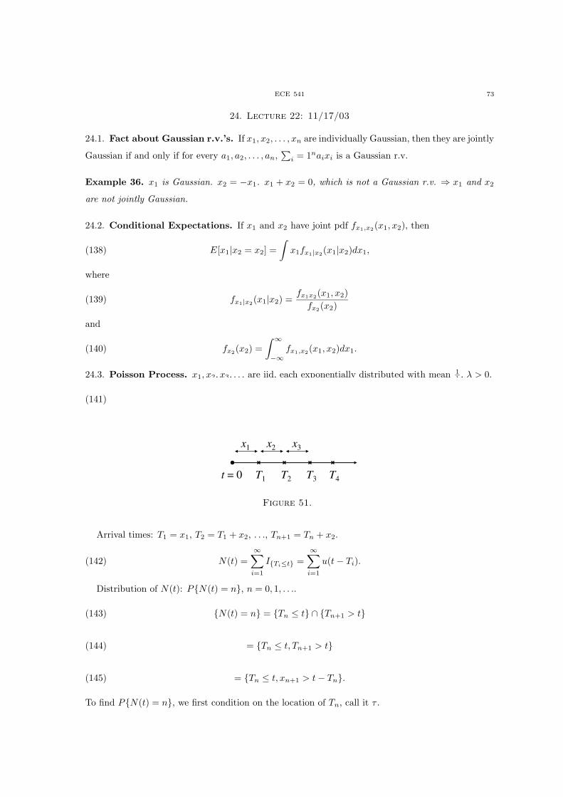
ECE 541 73

24. Lecture 22: 11/17/03

24.1. Fact about Gaussian r.v.’s. If x1, x2, . . . , xn are individually Gaussian, then they are jointly

Gaussian if and only if for every a1, a2, . . . , an,∑

i = 1naixi is a Gaussian r.v.

Example 36. x1 is Gaussian. x2 = −x1. x1 + x2 = 0, which is not a Gaussian r.v. ⇒ x1 and x2

are not jointly Gaussian.

24.2. Conditional Expectations. If x1 and x2 have joint pdf fx1,x2(x1, x2), then

(138) E[x1|x2 = x2] =

∫

x1fx1|x2(x1|x2)dx1,

where

(139) fx1|x2(x1|x2) =

fx1x2(x1, x2)

fx2(x2)

and

(140) fx2(x2) =

∫ ∞

−∞fx1,x2

(x1, x2)dx1.

24.3. Poisson Process. x1, x2, x3, . . . are iid, each exponentially distributed with mean 1λ , λ > 0.

(141) fx1(x) = λe−λxu(x).

x1

T2

x2 x3

T1 T3 T4t = 0

Figure 51.

Arrival times: T1 = x1, T2 = T1 + x2, . . ., Tn+1 = Tn + x2.

(142) N(t) =

∞∑

i=1

ITi≤t =

∞∑

i=1

u(t − Ti).

Distribution of N(t): PN(t) = n, n = 0, 1, . . ..

(143) N(t) = n = Tn ≤ t ∩ Tn+1 > t

(144) = Tn ≤ t, Tn+1 > t

(145) = Tn ≤ t, xn+1 > t − Tn.

To find PN(t) = n, we first condition on the location of Tn, call it τ .

74 MAJEED M. HAYAT

t-τ

τ = Tn0t

Figure 52.

We want xn+1 > t − τ (⇒ next arrival time falls beyond t). The range of τ is [0, t].

(146) PN(t) = n =

∫ t

0

fTn(τ)dτPxn+1 > t − τ.

We can do this because xn+1 and Tn are independent.

(147) Pxn+1 > t − τ =

∫ ∞

t−τ

fxn+1(x)dx =

∫ ∞

t−τ

λe−λxdx = e−λ(t−τ).

What is fTn?

(148) Tn = x1 + x2 + . . . + xn.

(149) fTn(τ) = fx1

(τ) ∗ . . . ∗ fxn(τ) =

(λτ)n−1λ

(n − 1)!u(τ).

(150) PN(t) = n =

∫ t

0

τn−1λn

(n − 1)!e−λτe−λ(t−τ)dτ

(151) = λne−λt

∫ t

0

τn−1

(n − 1)!dτ

(152) =(λt)ne−λt

n!, n = 0, 1, 2, . . . .

∴ N(t) is a Poisson r.v. with mean λt, where λ is the average rate of arrival. N(t) is called a Poisson

process. E[N(t)] = λt. We think of λ as the average rate of arrival. E[N 2(t)] = (λt)+(λt)2 because

var(N(t)) = λt.

Signal to Noise Ratio (SNR):

(153) SNR =E[N(t)]

σN (t)=

λt√λt

=√

λt.

σN (t) is the uncertainty. As t , the uncertainty (variability).

(154) RNN (t1, t2) = E[N(t1)N(t2)]; t1 ≤ t2

(155) = E[N(t1)N(t2) − N(t1) + N(t1)]

(156) = E[N(t1)N(t2 − N(t1) + N(t1)2]

ECE 541 75

(157) = λt1λ(t2 − t1) + λt1 + (λt1)2

(158) = λ2t1t2 − λ2t21 + λt1 + λ2t21

(159) = λt1 + λ2t1t2.

(160) KNN (t1, t2) = RNN (t1, t2) − E[N(t1)]E[N(t2)]

(161) = λt1 + λ2t1t2 − λ2t1t2 = λt1.

If t1 > t2,

(162) KNN (t1, t2) = λt2.

(163) ∴ KNN (t1, t2) = λmin(t1, t2).

24.4. Hazard or Failure Rates. Consider x1(= T1). Mean arrival time of 1λ . If we know that

x1 > x, what is the probability that it comes in [x, x + ∆x]? The probability is:

(164) Px < x1 ≤ x + ∆x|x1 > x =Px < x1 ≤ x + ∆x, x1 > x

Px1 > x

(165)Px < x1 ≤ x + ∆x, x1 > x

1 − Px1 ≤ x ≈ fx1(x)∆x

1 − Fx1(x)

(166) =

(

fx1(x)

1 − Fx1(x)

)

∆x.

(167) lim∆x→0

Px < x1 ≤ x + ∆x|x1 > x∆x

=fx1

(x)

1 − Fx1(x)

≡ a(x).

If fx1(x) = λe−λxu(x) then

(168) a(x) =λe−λxµ(x)

e−λxµ(x)= λ.

Conclusion: λ, which we interpreted as a mean arrival rate, is actually a failure rate (hazard

rate). That is, λ = a(

a = fx(x)1−Fx1

(x)

)

.

Conversely: If we know the failure rate of some phenomenon, call it a(x), what is the density

function fx1(x)? a(x) = fx(x)

1−Fx(x) .

(169)

∫ x

0

a(u)du =

∫ x

0

f(u)

1 − F (u)du = − log(1 − F (u))|x0

(170) = − log(1 − F (x)) + log(1 − F (0)) = − log(1 − F (x)).

(171) ⇒ 1 − F (x) = e−∫ x0

a(u)du.

76 MAJEED M. HAYAT

(172) ∴ F (x) = 1 − e−∫ x0

a(u)du

and

(173) f(x) = a(x)e−∫ x0

a(u)du.

Example 37. If a(x) = a, then fx(x) = ae−axu(x).

(174) a(x) =

λ, x ≥ xd

0, x < xd

(175) ⇒ fx(x) = λe−λ(x−xd)u(x − xd).

λ

a(x)

xd

Figure 53.

x

fx(x)

xd

Figure 54.

Processn

P

K=0 K=1 K=2

Figure 55. Some fail with probability p. µ(n) is the average time % load n.

ECE 541 77

25. Lecture 23: 11/19/03

25.1. Linear Estimation: Discrete Case. Disturbance Model:

ssignal(r.v.)

Distortion+ Noise xi

indexed by ii=1,2,…,n

Figure 56.

Question: Estimate s from x1, x2, . . . , xn. A simple approach: Form a linear function of the data

(linear estimator). What is the best linear estimator that we can get? In what sense? In the sense

of minimizing the mean-square error (MSE).

Problem: Find the coefficients, a1, . . . , an, such that

(176) MSE = E

(

s −n∑

i=1

aixi

)2

is minimized.

Solution: Method: Take dMSEdaj

= 0,∀j.

(177)d

daj

E

(

s −n∑

i=1

aixi

)2

= E

d

daj

(

s −n∑

i=1

aixi

)2

(178) = E

[

−2

(

s −n∑

i=1

aixi

)

xj

]

= 0.

(179) ∴ E[sxj ] = E

[

n∑

i=1

aixixj

]

.

Call E[sxj ] = Roj . Rij = E[xixj ], for any j. We can write it in matrix form: Ro = ~aR, where

~Ro = [R01R02 . . . Ron], for any j. ~a = [a1 . . . an]. We had seen that unless the xi’s are degenerate,

R is positive definite (hence invertible). ∴ ~a = ~RoR−1.

Example 38. Discrete Case: xi = S + Ni, i = 1, 2, . . . , n. s = a1x1 + . . . + anxn. Ro = aR.

(180) R =

σ2N + s2 s2 . . .

s2 σ2N + s2 . . .

. . . . . .. . .

.

(181) Ro =

s2

...

s2

.

78 MAJEED M. HAYAT

(182) s2 · · ·

1

1...

1

=

a1

...

an

σ2N + s2 . . . . . .

. . . σ2N + s2 . . .

. . . . . .. . .

.

(183) s2 = a1(σ2 + s2) + a2s

2 + . . . + ans2.

(184) s2 = a1s2 + a2(σ

2 + s2) + . . . .

(185) 1 = a1

(

σ2 + s2

s2

)

+ a2 + . . . + an.

(186) 1 = a1 + a2

(

σ2 + s2

s2

)

+ . . . + an.

(187) 0 = a1

(

σ2

s2

)

− σ2

s2a2 ⇒ a1 = a2 ⇒ a1 = a2 = . . . = an =

1

n.

Recall that we had:

(188) E[sXj ] = E

[

n∑

i=1

aixixj

]

.

(189) E

[

xj

(

s −n∑

i=1

aixi

)]

= 0, ∀j.

Error is orthogonal to the data that generated s (the estimate). This is known as the Orthogonality

Principle.

s(t)signal

degradation x(t)datainput

ht )(ˆ ts

Figure 57.

25.2. Linear Estimation: Continuous Case.

(190) s(t) =

∫ b

a

X(α)ht(α)dα.

This is a linear estimate of s(t) using the data in [a, b].

Question: What is the best ht(α) that minimizes MSE = E[(s(t) − s(t))2] for a fixed a, b, t.

Answer: Such an Rt(α) must satisfy the orthogonality principle. That is

(191) E

[(

s(t) −∫ b

a

x(α)ht(α)dα

)

x(τ)

]

= 0,∀τ ∈ [a, b].

ECE 541 79

~Ro = ~aR is called the Wiener-Hopf Equation.

Suppose that we are interested in a time-invariant filter ht(·). That is, ht(·) = ht(t − ·). Then

the Wiener-Hopf equation becomes

(192) E

[(

s(t) −∫ b

a

h(t − α)x(α)dα

)

x(τ)

]

= 0, τ ∈ [a, b].

(193) ∴ RSX(t, τ) =

∫ b

a

h(t − α)RXX(α, τ)dα, τ ∈ [a, b].

If s(t) is WSS, x(t) is WSS, then s is also WSS.

(194) RSX(t, τ) = RSX(t − τ).

(195) RXX(α, τ) = RXX(α − τ) = RXX(τ − α).

∴ with stationarity assumptions:

(196) RSX(t − τ) =

∫ b

a

h(t − α)RXX(τ − α)dα, ∀τ ∈ [a, b]( Wiener-Hopf equation).

Special case: Non-causal Wiener filter. a = −∞, b = +∞.

(197) RSX(t − τ) =

∫ ∞

−∞h(t − α)RXX(τ − α)dα, τ ∈ (−∞,∞).

Pick τ = 0 (no loss of anything).

(198) RSX(t) =

∫ ∞

−∞h(t − α)RXX(α)dα = h(t) ∗ RXX(t).

(199) SSX(ω) = H(ω)SXX(ω).

(200) H(ω) =SSX(ω)

SXX(ω)Non-causal Wiener filter.

Example 39.

(201) H(ω) =SSX(ω)

SXX(ω)= ?

s(t)WSS

x(t)data

h(t) )(ˆ ts

v(t)White Gaussian Noise (WGN)

+ x(t)

Observation Model Reconstruction(Restoration)

Figure 58.

80 MAJEED M. HAYAT

Find RSX(τ) first:

(202) RSX(τ) = E[s(t)x(t + τ)]

(203) = E[s(t)(s(t + τ) + v(t))] = RSS(τ).

(204) ∴ SSX(ω) = SSS(ω),

which is assumed to be known.

(205) SXX(ω) = FRSS(τ) + RV V (τ) = SSS(ω) + 1

(206) ⇒ H(ω) =SSS(ω)

1 + SSS(ω).

Example 40.

(207) H(ω) =SSX(ω)

SXX(ω).

s(t)WSS

x(t)data

h(t) )(ˆ ts

v(t)

+ x(t)g(t)

“blur”

Figure 59.

(208) RSX(τ) = E[s(t)x(t + τ)]

(209) = E[s(t)((s ∗ g)(t + τ) + v(t + τ))]

(210) = E

[

s(t)

∫ ∞

−∞s(t + τ − α)g(α)dα

]

(211) = RSS(τ) ∗ g(−τ).

(212) ∴ SSX(ω) = G ∗ (ω)SSS(ω).

Similarly,

(213) SXX(ω) = |G(ω)|2SSS(ω) + SV V (ω),

ECE 541 81

(214) ⇒ H(ω) =G ∗ (ω)SSS(ω)

|G(ω)|2SSS(ω) + SV V (ω).

(215) RXX(τ) = RSS(τ) ∗ g(−τ) ∗ g(τ).

82 MAJEED M. HAYAT

26. Lecture 24: 11/24/03

26.1. Linear Filtering. Non-causal optimal filter:

(216) s(t) =

∫ ∞

−∞hnc(t − τ)x(τ)dτ.

x: data, RXX known. s: signal, RSS known, RSX known. If

(217) Hnc(ω) =SSX(ω)

SXX(ω),

then

(218) E2 = E[(s(t) − s(t))2]

is minimized over all other LTI filters h(·). We used an orthogonality principle: Error ⊥ data used

to generate estimate, i.e.,

(219) E[(s(t) − s(t))] = 0,∀τ.

26.2. Causal Wiener Filtering. We want:

(220) s(t) =

∫ t

−∞h(t − τ)x(τ)dτ.

So, we want h(·) that minimizes the MSE,

(221) E2 = E[(s(t) − s(t))2].

Call the filter h(·). Use the orthogonality principle:

(222) E[(s(t) − (s)(t))x(τ)] = 0,∀τ ≤ t.

(223) ∴ RSX(t − τ) = E[s(t)x(τ)]

(224) = E

[∫ ∞

−∞h(t − α)x(α)dαx(τ)

]

(225) =

∫ t

−∞h(t − α)RXX(α − τ)dα, τ ≤ t.

Change of variable: u = t − α.

(226) ⇒ RSX(t − τ) =

∫ ∞

0

h(u)RXX(t − u − τ)du, τ ≤ t.

True when τ = 0. Call η = t − τ .

(227) RSX(η) =

∫ ∞

0

h(u)RXX(η − u)du, η ≥ 0

(228) =

∫ ∞

−∞h(u)RXX(η − u)du, η ≥ 0.

ECE 541 83

(Looks like convolution, but only for positive η, its not a convolution ⇒ cannot apply Fourier

Transform). For the moment, suppose RXX(τ) = δ(τ). Equation (228) gives: RSX(τ) = h(τ), τ ≥ 0,

but h(τ) = 0, if τ < 0 by causality.

(229) ∴ h(t) = RSX(t)u(t).

Real problem:

Not WhiteY(t)

WSSoriginal data

whiteningfilter

Whitex(t)

transformed data

)(ˆ ts

)(tγ

)()( tutRSX

hc(t)

Figure 60.

(230) hc(t) = γ(t) ∗ (RSX(t)u(t)).

(231) hc(t) = γ(t) ∗ [(RSY (t) ∗ γ(−t))u(t)].

Error Calculation:

(232) MSE = E[(s(t) − s(t))2] = E[(s(t) − s(t))(s(t) − s(t))]

(233) = −E[(s(t) − s(t)s(t)]

because s(t) is orthogonal to (s(t) − s(t)).

(234) MSE = RSS(0) − E[s(t)s(t)]

(235) = RSS(0) − E[s(t)s(t)]

(236) = RSS(0) − E

[

s(t)

∫ t

−∞x(u)RSX(t − u)du

]

(237) = RSS(0) −∫ t

−∞RSX(t − u)RSX(t − u)du.

y = t − u.

(238) = RSS(0) −∫ ∞

0

R2SX(y)dy

84 MAJEED M. HAYAT

(239) MSE = RSS(0) −∫ ∞

0

[(RSY (y) ∗ γ(−y))u(y)]2dy.

What about γ(t)? SXX(ω) = 1. SY Y (ω)|Γ(ω)|2 = 1. ∴ |Γ(ω)|2 = 1SY Y (ω) . It turns out that:

γ(t) )(txY(t)white

Figure 61.

(240)1

SY Y (ω)= Γ(jω)Γ(−jω).

Example 41.

(241) Y (t) = s(t) + v(t),

where Y (t) is data, s(t) is WSS, v(t) is WGN and s and v are uncorrelated.

(242) SSS(ω) =12

4 + ω2.

SV V (ω) = 1 (w/rad/s).

Find hc(t) and the error.

(243) hc(t) = γ(t) ∗ [RSY (t) ∗ γ(−1)]u(t).

(244) SY Y (ω) = SSS(ω) + SV V (ω)

(245) =16 + ω2

4 + ω2=

(4 + jω)(4 − jω)

(2 + jω)(2 − jω)

(246) = Γ−1(jω)Γ−1(−jω).

(247) ∴ Γ(jω) =2 + jω

4 + jω: causal.

(248) Γ(s) =2 + jω

4 + jω= 1 − 2

s + 4.

(249) γ(t) = s(t) − 2e−4tu(t) : causal.

Compute RSY (t).

(250) RSY (t) = RSS(t) = F−1

12

4 + ω2

(251) L−1

12

4 − s2

= L−1

3

s + 2+

3

s − 2

.

ECE 541 85

RSY (t) ∗ γ(−t), i.e., SSY (s)Γ(−s),

(252) = L−1 SSY (s)Γ(−s)

(253) = L−1

12

4 − s2

2 − s

4 − s

(254) = L−1

12

(2 − s)(s + 2)

2 − s

4 − s

= L−1

12

(2 + s)(4 − s)

.

(255) (RSY (t) ∗ γ(−1))u(t) = L−1

12

(2 + s)(4 − s)

: causal

(256) = L−1

2

2 + s+

2

4 − s

(257) = 2e−2tu(t).

(258) hc(t) = [(RSY (t) ∗ γ(−t))u(t)] ∗ γ(t) = 2e−2tu(t) ∗ (δ(t) − 2e−4tu(t)).

(259) Hc(s) =2

s + 2

[

2 + s

4 + s

]

=2

4 + s.

(260) ∴ hc(t) = 2e−4tu(t).

(261) MSE = RSS(0) −∫ ∞

0

[RSX(t)]2dt

(262) = 3 −∫ ∞

−∞(2e−2tu(t))2dt = 2

(263) RSS(τ)F−1

12

4 + ω2

= 3e−2|τ |.

86 MAJEED M. HAYAT

27. Lecture 25: 11/26/03

27.1. Spectral Factorization. A power spectral density (PSD) can be thought of as the PSD of

the output of an LTI system with white noise as its input.

H )(tYW(t)(w/rads)

20N

Figure 62. H is a ratio of polynomials.

(264) SY Y (ω) = |H(ω)|2 N0

2.

We can write:

(265) H(ω) =A(ω2) + jωB(ω2)

C(ω2) + jD(ω2),

where A,B,C and D are polynomials with real coefficients.

(266) ∴ |H(ω)|2 =A2(ω2) + ω2B2(ω2)

C2(ω2) + ω2D2(ω2).

∴ |H(ω)|2 is a ratio of two polynomials that are even and have real coefficients.

Consequence 1: Because the coefficients are real, zeros and poles of |H|2 occur with conjugate

symmetry if complex. That is, if s = σ + jω is a pole (zero), then so is s∗ = σ − jω.

Consequence 2: Because we have even polynomials in |H(ω)|2, if s is a pole or zero, so is −s.

consequence 2

consequence 1

Figure 63.

∴ we can write:

(267) s(ω) = S(s)|s=jω =

∏

p(s − sp)∏

k(s − sk)

ECE 541 87

(268) = φ−(s)φ+(s),

where φ+(s) = φ−(s) and S(ω) = |φ+(ω)|2 = |φ−(ω)|2. In particular, φ+ is stable and 1φ+ is also

stable.

Example 42.

(269) S(ω) =2ω2 + 3

ω2 + 1=

√2(jω +

√

3/2)(jω −√

3/2)√

2

(jω + 1)(jω − 1).

(270) φ+(s) =

√2(s +

√

3/2)

s + 1.

(271) φ−(s) =

√2(s −

√

3/2)

s − 1.

27.2. Optimal Linear Prediction. We want the following: λ > 0. Estimate s(t + λ) using the

data x(τ) in the range τ ∈ [−∞, t]. We do it in a linear fashion:

(272) s(t + λ) =

∫ ∞

0

x(t − α)h(α)dα,

where h(α) is a causal filter. Equivalently,

(273) s(t) =

∫ ∞

0

x(t − λ − α)h(α)dα.

We can think of this equation as a causal Wiener filter but with delayed data (delay is a linear

transformation). What is the optimal h? We appeal to the orthogonality principle: error ⊥ data.

(274) e(t + λ) = s(t + λ) − s(t + λ).

(275) E[(s(t + λ) − s(t + λ))x(α)] = 0, ∀α ≤ t.

We obtain:

(276) RSX(t + λ − α) = RSX(t + λ − α), ∀α ≤ t.

(277) RSX(τ) = E

[∫ ∞

0

h(α)x(τ − λ − α)dαx(τ)

]

.

(278) RSX(τ + λ) =

∫ ∞

0

h(α)RXX(τ − α)dα.

Let β = t − α. This gives:

(279) RSX(λ + β) = RSX(λ + β), β ∈ [0,∞)

(280) =

∫ ∞

0

h(α)RXX(β − α)dα.

88 MAJEED M. HAYAT

(281) RSX(β) =

∫ ∞

0

h(α)RXX(β − λ − α)dα.

Solution:

(282) hw(t) = γ(t) ∗ [RSY (t + λ) ∗ γ(−t)]u(t).

The +τ term is the difference with causal h(t).

)(tγ

SYR)(tγ

)( λ+tRSY

λ

)]()()[( ttRtu SY −∗+ γλ

Form: )()( ttRSY −∗+ γλ

Figure 64.

27.3. Smoothing. λ < 0.

(283) s(t + λ) =

∫ ∞

0

h(α)x(t − α)dα.

In this case, we move RSY to the right by λ. Let x′ be a delayed version of x. The ingredient in

the causal Wiener filter was RSX (we can use RSX′), we only care about correlation between s and

data. But, RSX′(τ) = RSX(τ) ∗w(−τ), where w(τ) = δ(t− λ) : delay. Linear estimation: Filtering,

prediction and smoothing.

27.4. Markov Chains. x0 x1 . . . xn . . . (discrete valued) is a Markov chain if

(284) Pxn = j|x1 = i1, x2 = i2, . . . , xn−1 = in−1 = Pxn = j|xn−1 = in−1.

Example 43. Gambling: Initial fortune = x0 = Xo. Each time we either increment our fortune or

decrement (with probability p). Let xn denote the fortune at time n.

(285) Pxn = j|x1 . . . xn−1 = Pxn = j|xn−1.

ECE 541 89

Problem: Suppose that we start gambling if we reach a goal. Xo = xo. xmax = goal. You also

stop whenever you loose all of your money. Let P (x) be the probability of achieving your goal, where

x is the initial fortune. Also, p is the probability of winning a hand. Recipe for P (x): P (0) = 0.

(286) P (x) = pP (x + 1) + (1 − p)P (x − 1).

(287) x = 0, 1, 2, . . . , xmax.

90 MAJEED M. HAYAT

28. Lecture 26: 12/01/03

28.1. Linear Prediction. X(t) WSS data, conveys information on s(t) (WSS). We want to predict

s(τ + λ) using data in the range (−∞, t).

(288) s(t + λ) =

∫ ∞

0

h(α)x(t − α)dα.

Orthogonality principle:

(289) e(t + λ) ⊥ x(t − α), α ≥ 0.

(290) e(·) = s(·) − s(·).

(291) E[s(t + λ) − s(t + λ)x(t − α)] = 0, ∀α ≥ 0.

(292)

∫ ∞

0

h(β)RXX(α − β)dβ = RSX(λ + α), α ≥ 0.

If x was white (RXX(α − β) = δ(α − β)), then

(293) h(α) = RSX(λ + α)u(t), α ≥ 0.

x IWhite

)(ˆ λ+ts)(tγIh

h(t)

Figure 65.

But,

(294) RSI(t) = RSX(t) ∗ γ(−t).

∴ the total

(295) h(t) = hI(t) ∗ γ(t).

Recipe:

(296) h(t) = (RSX ∗ γ(−·))(λ + t)u(t) ∗ γ(t).

Error:

(297) ε = E[e2(t + λ)] = −E[s(t + λ) − s(t + λ)s(t + λ)]

ECE 541 91

(298) = RS(0) − E

[∫ ∞

0

h(α)x(t − α)s(t + λ)dα

]

(299) = RS(0) −∫ ∞

0

h(α)RSX(λ + α)dα

(300) = RSS(0) −∫ ∞

0

h2I(α)dα.

Example 44.

(301) SSS(s) =49 − 25s2

(1 − s2)(9 − s2)= SXX(s).

No noise:

(302) SSS(s) =(7 + 5s)(7 − 5s)

(1 + s)(3 + s)(1 − s)(3 − s).

(303) Γ(s) =(1 + s)(3 + s)

(7 + 5s).

(304) hI(t) = RSI(λ + t)u(t) = [RSX(λ + t) ∗ γ(λ + t)]u(t)

(305) = [RSS(λ + t) ∗ γ(−(λ + t))] ∗ u(t).

In our case, RSX = RSS.

(306) SSI(s) = SSS(s)Γ(−s) =1

Γ(s).

Recall that

(307) hI(t) = RSI(λ + t)u(t).

Put

(308) L−1

1

Γ(s)

=∑

i

ciesitu(t).

(309) RSI(λ + t) =∑

i

ciesi(t+λ)u(t).

(310) u(t)RSI(λ + t) =∑

i

ciesi(t+λ)u(t).

(311) HI(s) =c1

s − s1esiλ +

c2

s − s2es2λ

∣

∣

∣

s1=−1

s2=−3

∣

∣

∣

c1=1

c2=4.

(312) HI(s) =e−λ

s + 1+

4e−3λ

s + 3

∣

∣

∣

λ=log 2

(313) =s + 2

(s + 1)(s + 3).

92 MAJEED M. HAYAT

(314) h(t) = γ(t) ∗ hI(t).

(315) H(s) = Γ(s)HI(s)

(316) =(1 + s)(3 + s)(s + 2)

(7 + 5s)(s + 1)(s + 3)=

s + 2

7 + 5s.

(317) h(t) = 0.2δ(t) +3

25e−1.4tu(t).

(With noise, we will have a different RSI .)

28.2. Markov Chains. Let Q(x) be the probability of winning if we start with fortune x.

n0

x

xmax

Figure 66.

(318) Q(x) = pQ(x + 1) + qQ(x + 1),

where p is the probability of winning the first hand and q is the probability of losing the first hand.

Q(0) = 0. Q(xmax) = 1. Propose a solution of the form rx and plug it in.

(319) rx = prx+1 + qrx−1.

(320) rx+1 = prx+2 + qrx.

(321) r = pr2 + q.

(322) r2 +q

p− r

p= 0.

(323) r1,2 =1 ±

√

1 − 4p(1 − p)

2p.

If r1 6= r2,

(324) Q(x) = Arx1 + Brx

2 .

ECE 541 93

Apply the initial conditions,

(325) Q(x) =1

rxmax1 − rxmax

2

(rx1 − rx

2 ).

1 = r1 = r2 when p = 12 .

(326) Q(x) = A + Bx.

Apply initial conditions:

(327) Q(x) =x

xmax.

Let xn denote the fortune at time n.

(328) winning = xi = xmax,∀i.

Also, if winning occurs, then

(329) xi = xmax, infinitely many times occurs.

(330) winning = xi = xmax, infinitely often.

(331) loose = xi = 0, infinitely often.

We just proved that

(332) Pxi = xmax, infinitely often =x

xmax.

(333) Pxi = 0, infinitely often = 1 − x

xmax,

by doing the same analysis, for the probability of losing as we did for Q(x). These two imply that

(334) P limn→∞

xn = xmax =x

xmax.

(335) P limn→∞

xn = 0 = 1 − x

xmax.

(336) P ( limn→∞

xn 6= 0 ∪ limn→∞

xn 6= xmax) = 0.

∴ we proved that limn→∞ xn = x, where x is 0, xmax-valued and Px = 0 = 1 − xxmax

.

(337) P limn→∞

xn = x = 1

(338) ⇒ xn → x almost surely.

94 MAJEED M. HAYAT

28.3. Martingales. A sequence x1, x2, . . . is a martingale if E[xn+k|xn] = xn. If we consider the

gambler’s example, the fortune “xn” is a martingale if p = 12 . If the condition E[xn+k|xn] = xn is

replaced by ≤ (≥), we call xn a super (sub) martingale.

Theorem 10. Martingale Convergence Theorem. If xn is a sub-, super-, or martingale and E[|x1|] <

∞, then xn converges to a r.v. almost surely.

In real numbers, if xn with a property that |xn| < B < ∞, xn+1 ≥ xn, then xn is convergent

(from Completeness of Real Numbers, the Bolzano-Weirstrass Theorem).

(339) E[xn+1|xn] ≥ xn ⇒ E[xn+1] ≥ E[xn].

28.4. Markov Chains. Back to the gambling problem.

(340) Pij = Pxn+1 = j|xn = i =

p, if j = i + 1, i 6= xmax

q, if j = i − 1, i 6= 0

1, if i = j = xmax

1, if i = j = 0

Define the probability transition matrix P = ((Pij)). For our example:

(341) P =

1 0 0 . . . . . . . . . . . . . . . 0

q 0 p 0 . . . . . . . . . . . ....

0 q 0 p 0 . . . . . . . . ....

......

......

.... . .

......

...

0 0 . . . . . . . . . . . . q 0 p

0 0 . . . . . . . . . . . . . . . . . . 1

.

P has the property that the sum of any row is 1, which is called a stochastic matrix.

Exercise 11. Show that λ = 1 is always an eigenvalue for any stochastic matrix P.

(342) Ax = λx ⇒ xP = λx.

ECE 541 95

29. Lecture 27: 12/03/03

29.1. Gambler’s Ruin Problem. if p = q = 12 ,

(343) Q(x) =x

xmax,

(344) P (x) = 1 − x

xmax

and

(345) limxmax→∞

P (x) = 1.

Similarly, one can argue that with probability 1, the party with no capital limitation wins. In fact,

as long as q ≥ p, the limxmax→∞ P (x) = 1.

Exercise 12. Show that

(346) limxmax→∞

P (x) = 1

when q ≥ p.

Aside: Back to the Martingale Convergence Theorem.

(347) supn

E[|xn|] < ∞,

then xn → x a.s, where xn is a Martingale sequence and x is a r.v.

Markov Chain: xo x1 x2 . . .. xo is a r.v. with distribution Po : Poxo = i = Po(i). Define

(348) Pij = Pxn+1 = j|xn = i.

P = ((Pij)).

(349) Pxx+2 = j|xn = i =∑

k

Pxn+2 = j, xn+1 = k|xn = i.

Use Bayes Identity:

(350) P (A ∩ B|C) = P (A|B ∩ C)P (B|C).

(351)∑

k

Pxn+2 = j ∩ xn+1 = k|xn = i ∩ xn+1 = kPxn+1 = k|xn = i

(352) =∑

k

Pxn+2 = j|xn = i, xn+1 = kPxn+1 = k|xn = i

(353) =∑

k

Pxn+2 = j|xn+1 = kPxn+1 = k|xn = i

(354) =∑

k

PikPkj = (P × P)i,j = P2i,j .

96 MAJEED M. HAYAT

More generally,

(355) Pxn+k = j|xn = i = Pn(i, j).

∴ Pk is the k-step transition probability matrix.

Back to Gambler’s ruin problem: xmax = 4, p = 0.6 and q = 0.4.

(356) P =

1 0 0 0 0

0.4 0 0.6 0 0

0 0.4 0 0.6 0

0 0 0.4 0 0.6

0 0 0 0 1

.

Regression: Also, we know that Pn = PkP`, where ` + k = n.

Back to problem:

(357) P2 =

1 0 0 0 0

0.4 0.24 0 0.36 0

0.16 0 0.48 0 0.36

0 0.16 0 0.24 0.6

0 0 0 0 1

.

(358) limn→∞

Pn =

1 0 0 0 0

0.5846 0 0 0 0.4154

0.3077 0 0 0 0.6923

0.1231 0 0 0 0.8769

0 0 0 0 1

.

(Use Spectral Theorem to solve). Note that the last column is

(359) Q(x) =

Q(0)...

Q(4)

.

In our case,

(360) Po =[

0 0 1 0 0]

.

In particular,

(361) (PoP∞)xmax

= (Q(x))xmax

(362) → limn→∞

xn = xmax|xo = x.

ECE 541 97

(363) Pn = Pxn = j = Po,Pn = P1P

n−1 = P2Pn−2 = . . . = Pn−1P.

But, what is the limit as n → ∞ of Pn?

(364) limn→∞

Pn = PoP∞.

∴ Pn = Pn−1P.

(365) limn→∞

Pn = ( limn→∞

Pn−1)P.

(366) π = πP,

where π is the probability mass function of where you are in the future. π is a left eigenvector of P

corresponding to eigenvalue 1.

Consider:

P21

P22

P12

upstate1

P11

downstate0

Figure 67.

(367) P =

p11 p12

p21 p22

=

0.9999 0.0001

0.01 0.99

.

(368) limn→∞

Pn =

0.9901 0.0099

0.9901 0.0099

.

Rows are identical: meaning the initial state does not affect the state in the limit as n → ∞.

P (up at n = ∞) = 0.9901. P (down at n = ∞) = 0.0099.

(369) Pxn = i = (PoP)ith component.

(370) πn =

Pxn = 1Pxn = 0

= PoPn.

Take limits:

(371) limn→∞

πn = limn→∞

PoPn

98 MAJEED M. HAYAT

(372) = ( limn→∞

πn−1)P.

(373) π = πP.

(374) ∴ limn→∞

Pn =

π...

π

.

Suppose that Po = π.

(375) π1 = PoP = πP = π.

(376) π2 = PoP2 = PoPP = πP = π.

(377)...

(378) πn = π.

∴ π is called a stationary distribution.

Finding π: Set π = πP.

(379)[

π1 π2

]

=[

π1 π2

]

P11 P12

P21 P22

.

(380) π1 = P11π1 + P21π2 ∴ π1(1 − P11) = P21π2.

(381) π2 = P12π1 + P22π2 ∴ π1 =P21

1 − P11π2.

(382) π =

[

π11 − P11

P21π1

]

with the proviso that:∑

i πi = 1. ∴ π1 + 1−P11

P21π1 = 1.

(383) ∴ π1

(

1 +1 + P11

P21

)

= 1.

(384) π1 =P21

P21 − P11 + 1; π2 = 1 − π1.

Sufficient condition for existence of π: If every component is non-zero, then πP = π,∑

i πi = 1

has a unique non-zero solution called the stationary distribution of the Markov Chain. If

(385) P nii = Pxn = i|xo = i

and

(386) P nij = Pxn = j|xo = i,

ECE 541 99

then

(387) πi = limn→∞

Pnii = lim

n→∞Pn

ji.

A process x(t) is ergodic if

(388) E[x(t)] = limT→∞

1

2T

∫ T

−T

x(t)dt a.s.

100 MAJEED M. HAYAT

30. Lecture 28: 12/08/03

30.1. Sampling Theorem for Bandlimited Stochastic Processes.

30.1.1. The Deterministic Case. Let x(t) be a signal with x(f) = 0, ∀|f | > w, where

(389) x(f) =

∫ ∞

−∞x(t)e−j2πftdt.

W-W

X(f)I

Figure 68.

Define

(390) s(t) ,

∞∑

k=−∞δ(t − kT ).

Note that:

(391) s(f) =1

T

∞∑

k=−∞δ

(

f − k

T

)

.

T

s(t)

0

Figure 69.

Proof:

(392) s(t) =∑

k

δ(t − kT )

(393) =∑

k

Ckej 2πktT ,

where

(394) Ck =1

T

∫ T/2

−T/2

s(t)e−j 2πktT dt =

1

T· 1 =

1

T.

ECE 541 101

(395) s(t) =1

T

∑

k

ej 2πktT .

(396) ⇒ s(f) =1

T

∑

k

δ

(

f − k

T

)

.

1T ≥ 2W . Define xs(t) = x(t)s(t).

(397) xs(t) = x(t)∞∑

k=−∞δ(t − kT ) =

∑

k

x(kT )δ(t − kT ).

(398) xs(f) = Fx(t)s(t).

(399) xs(f) = X(f) ∗ S(f) = X(f) ∗ 1

T

∑

k

δ

(

f − k

T

)

.

(400) Xs(f) =1

T

∑

k

x

(

f − k

T

)

.

W-W

X(f)I

W-W

T1−

WT

−1W

T+1

Figure 70.

1T − W ≥ W . 1

T ≥ 2W so we have no overlap.

(401) H(f) = T rect(2Wf).

W-W

H(f)T

f

Figure 71.

(402) X(f) = H(f)Xs(f).

(403) x(t) = h(t) ∗ sx(t).

102 MAJEED M. HAYAT

(404) = h(t) ∗∑

k

x(tk)δ(t − kT ).

(405) =∑

k

x(kt)h(t − kT ).

(406) h(t) = F−1rect(2Wf) = 2WT sinc(2πWt).

(407) = 2WTsin(2πWt)

2πWt.

(408) x(t) = 2WT∑

k

x(kT )sin(2πW (t − kT ))

2πW (t − kT ).

Pick T = 12W or 1

T = 2W (Nyquist Rate).

(409) x(t) =∑

k

x(kT )sin(2πW (t − k

2W ))

2πW (t − k2W )

.

Question: Consider xto(t) = x(t − t0).

(410) xto(t) =

∑

k

xto(kT )

sin(2πW (t − k2W ))

2πW (t − k2W )

.

(411) xto(t) =

∑

k

xto(kT − to)

sin(2πW (t − k2W ))

2πW (t − k2W )

, ∀to.

If to = t,

(412) x(0) =∑

k

x(kT − t)sin(2πW (t − k

2W ))

2πW (t − k2W )

.

Remark: If x(t) is an energy signal, i.e.,∫

x2(t)dt < ∞, then the above representation of x(t)

says the following:

(413) limN→∞

∫

∣

∣

∣

∣

∣

x(t) −N∑

k=−N

x(kT )sin(2πW (t − k

2W ))

2πW (t − k2W )

∣

∣

∣

∣

∣

2

dt = 0.

30.1.2. The Stochastic Case. A process x(t) is said to be bandlimited to W , if its power spectral

density φ(f) = 0, ∀|f | > W .

W-W

(f)

Figure 72.

ECE 541 103

(414) φ(f) = limT→∞

E|FXT (t)|22T

.

(415) XT (t) =

X(t), |t| ≤ T

0, otherwise

From the Wiener-Kinchin relation,

(416) φ(f) = Fφ(τ),

where φ(τ) is a deterministic function.

(417) φ(τ) =∑

k

φ(kT )sin(2πW (t − k

2W ))

2πW (t − k2W )

.

30.2. Stochastic Sampling Theorem. If a WSS random process X(t) is bandlimited to the band-

width W , then upon setting T = 12W (Nyquist Rate)

(418) X(t) =∑

k

X(kT )sin(2πW (t − k

2W ))

2πW (t − k2W )

.

in the mean square sense, that is with

(419) XN (T ) ,

N∑

n=−N

X(nT )sin(2πW (t − k

2W ))

2πW (t − k2W )

.

Then,

(420) limN→∞

E(X(t) − XN (t))2 = 0, for each t.

Proof: We want to prove

(421) limN→∞

E(X(t) − XN (t))2 = 0

(422) = limN→∞

E(X(t) − XN (t))(X(t) − XN (t))

(423) = limN→∞

E[(X(t) − XN (t))X(t)] − E[(X(t) − XN (t))XN (t)]

(424) limN→∞

E[(X(t) − XN (t))X(t)] = E[X2(t)] − limN→∞

E[XN (t)X(t)]

(425) = φ(0) −∞∑

k=−∞E[X(t)X(kT )]

sin(2πW (t − k2W ))

2πW (t − k2W )

.

(426) = φ(0) −∞∑

k=−∞φ(kT − t)

sin(2πW (t − k2W ))

2πW (t − k2W )

.

(427) = φ(0) − φ(0) = 0.

104 MAJEED M. HAYAT

(428) XN (t) =N∑

n=−N

X(nT )sin(2πW (t − k

2W ))

2πW (t − k2W )

.

So, XN (t) is a weighted sum of x(mT ), so it is enough to show that

(429) limN→∞

E[(X(t) − XN (t))X(mT )] =? 0.

(430) limN→∞

E[(X(t) − XN (t))X(mT )] = E[X(t)X(mT )] − limN→∞

E[XN (t)X(mT )]

(431) = φ(t − mT ) −∞∑

n=−∞E[X(nT )X(mT )]

sin(2πW (t − k2W ))

2πW (t − k2W )

(432) = φ(t − mT ) −∞∑

n=−∞φ(nT − mT )

sin(2πW (t − nT ))

2πW (t − nT )

(433) = φ(t − mT ) − φ(t − mT ) = 0.

ECE 541 105

References

[1] Chow, Y. S. and H. Teicher, “Probability Theory: Independence, Interchangeability, Martingales,” Series:

Springer Texts in Statistics (New York), 3rd ed., 1997. ISBN: 0-387-40607-7.

[2] Clark, R. N., G. A. Swayze, K. E. Livo, R. F. Kokaly, S. J. Sutley, J. B. Dalton, R. R. McDougal and C. A. Gent,

“Imaging Spectroscopy: Earth and Planetary Remote Sensing with the USGS Tetracorder and Expert Systems,”

Journal of Geophysical Research, Inc., In Press 2003, http://speclab.cr.usgs.gov/PAPERS/tetracorder/.

[3] The Imaging Spectroscopy Lab at USGS: http://speclab.cr.usgs.gov/.