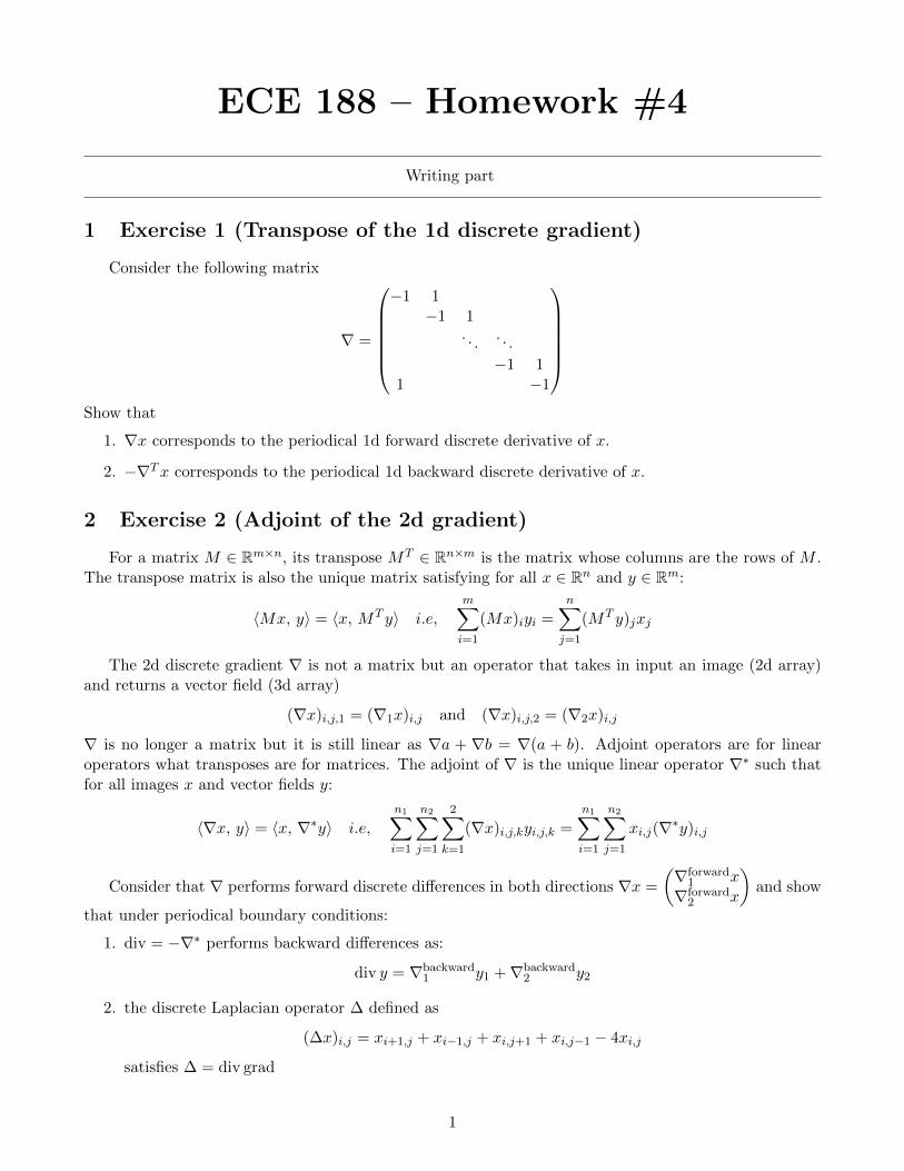
ECE 188 – Homework #4

Writing part

1 Exercise 1 (Transpose of the 1d discrete gradient)

Consider the following matrix

∇ =

−1 1

−1 1. . .

. . .

−1 11 −1

Show that

1. ∇x corresponds to the periodical 1d forward discrete derivative of x.

2. −∇Tx corresponds to the periodical 1d backward discrete derivative of x.

2 Exercise 2 (Adjoint of the 2d gradient)

For a matrix M ∈ Rm×n, its transpose MT ∈ Rn×m is the matrix whose columns are the rows of M .The transpose matrix is also the unique matrix satisfying for all x ∈ Rn and y ∈ Rm:

〈Mx, y〉 = 〈x, MT y〉 i.e,m∑i=1

(Mx)iyi =n∑

j=1

(MT y)jxj

The 2d discrete gradient ∇ is not a matrix but an operator that takes in input an image (2d array)and returns a vector field (3d array)

(∇x)i,j,1 = (∇1x)i,j and (∇x)i,j,2 = (∇2x)i,j

∇ is no longer a matrix but it is still linear as ∇a + ∇b = ∇(a + b). Adjoint operators are for linearoperators what transposes are for matrices. The adjoint of ∇ is the unique linear operator ∇∗ such thatfor all images x and vector fields y:

〈∇x, y〉 = 〈x, ∇∗y〉 i.e,

n1∑i=1

n2∑j=1

2∑k=1

(∇x)i,j,kyi,j,k =

n1∑i=1

n2∑j=1

xi,j(∇∗y)i,j

Consider that ∇ performs forward discrete differences in both directions ∇x =

(∇forward

1 x∇forward

2 x

)and show

that under periodical boundary conditions:

1. div = −∇∗ performs backward differences as:

div y = ∇backward1 y1 +∇backward

2 y2

2. the discrete Laplacian operator ∆ defined as

(∆x)i,j = xi+1,j + xi−1,j + xi,j+1 + xi,j−1 − 4xi,j

satisfies ∆ = div grad

1

Practical part

The following exercises should be done after completing the Matlab codes of Homework #3 andcommitting them. Once done switch the the branch homework4. This version of the code containsupdated and new files required for the following exercises. Merge them with your own progress fromHomework #3. Read carefully the messages, you may have conflicts. Solve all the conflicts, and committhe solved version before doing anything else.

3 Exercise 3 (Heat equation)

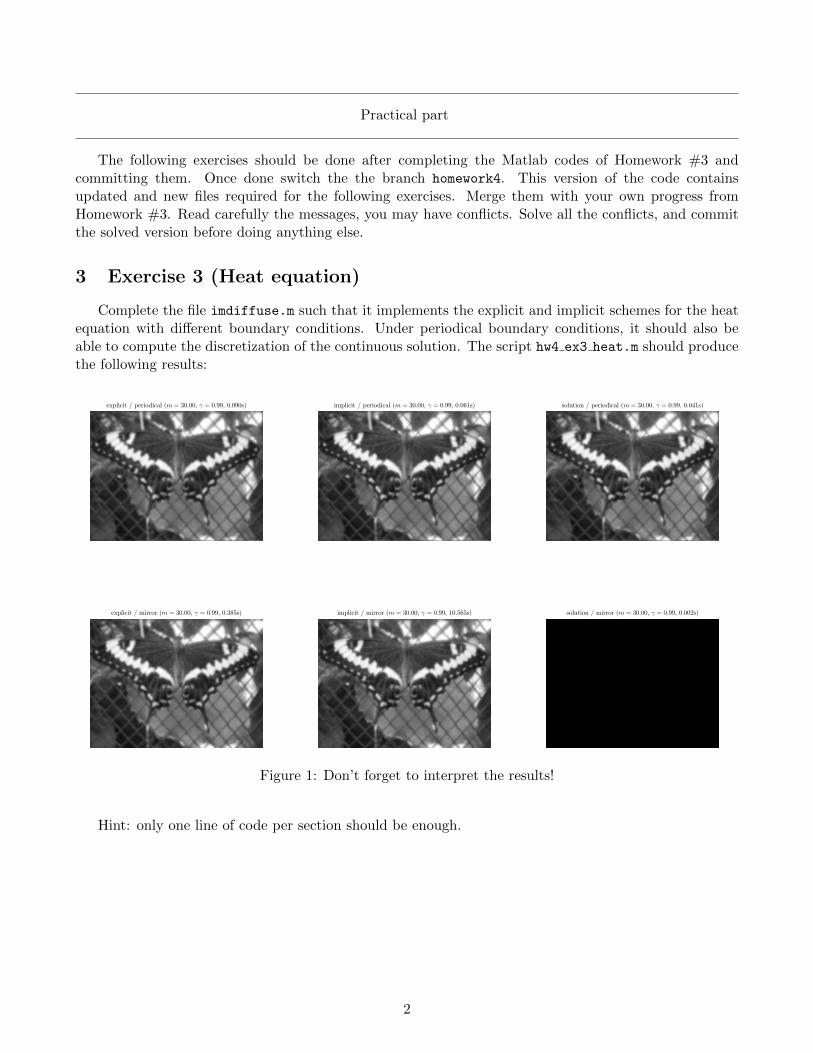
Complete the file imdiffuse.m such that it implements the explicit and implicit schemes for the heatequation with different boundary conditions. Under periodical boundary conditions, it should also beable to compute the discretization of the continuous solution. The script hw4 ex3 heat.m should producethe following results:

explicit / periodical (m = 30.00, γ = 0.99, 0.090s) implicit / periodical (m = 30.00, γ = 0.99, 0.061s) solution / periodical (m = 30.00, γ = 0.99, 0.041s)

explicit / mirror (m = 30.00, γ = 0.99, 0.385s) implicit / mirror (m = 30.00, γ = 0.99, 10.565s) solution / mirror (m = 30.00, γ = 0.99, 0.002s)

Figure 1: Don’t forget to interpret the results!

Hint: only one line of code per section should be enough.

2

4 Exercise 4 (Anisotropic diffusion)

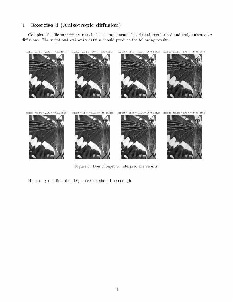
Complete the file imdiffuse.m such that it implements the original, regularized and truly anisotropicdiffusions. The script hw4 ex4 anis diff.m should produce the following results:

explicit / rad (m = 20.00, γ = 0.99, 2.061s) implicit / rad (m = 5.00, γ = 3.96, 8.014s) implicit / rad (m = 1.00, γ = 19.80, 1.609s) implicit / rad (m = 1.00, γ = 198.00, 1.597s)

explicit / tad (m = 20.00, γ = 0.99, 5.682s) implicit / tad (m = 5.00, γ = 3.96, 18.840s) implicit / tad (m = 1.00, γ = 19.80, 3.822s) implicit / tad (m = 1.00, γ = 198.00, 3.953s)

Figure 2: Don’t forget to interpret the results!

Hint: only one line of code per section should be enough.

3