ec487 advanced microeconomics, part i: lecture 1

EC487 Advanced Microeconomics, Part I:Lecture 1

Leonardo Felli

32L.LG.04

29 September, 2017

Course Outline

Microeconomic Theory

I Lecture 1: Production Theory and Profit Maximization.

I Lecture 2: Cost Minimization and Aggregation.

I Lecture 3: Pure Exchange Economy and WalrasianEquilibrium.

I Lecture 4: Existence of Walrasian Equilibrium and WelfareTheorems.

I Lecture 5: Walrasian Equilibrium with Production andExternalities.

Leonardo Felli (LSE) EC487 Advanced Microeconomics, Part I 29 September, 2017 2 / 55

Course Outline (cont’d)

Games of Complete Information

I Lecture 6: Static games and Nash Equilibrium.

I Lecture 7: Nash Theorem and Duopoly.

I Lecture 8: Dynamic Games, Subgame Perfection andBargaining Games.

I Lecture 9: Repeated Games.

I Lecture 10: The Folk Theorem.


Admin

I My coordinates: 32L.4.02, x7525, [email protected]

I PA: Emma Taverner, 32L.1.28, [email protected].

I Office Hours: Friday 11:00-13:00 or by appointment ([email protected]).

I Course Material: available at:http://econ.lse.ac.uk/staff/lfelli/teaching


http://econ.lse.ac.uk/staff/lfelli/teach/EC487.htm

Textbooks

I Andreu Mas-Colell, Michael Whinston and Jerry Green,Microeconomic Theory, Oxford: Oxford University Press,1995.

I Martin J. Osborne and Ariel Rubinstein, A Course in GameTheory M.I.T. Press, 1994.

I Drew Fudenberg and Jean Tirole, Games Theory, Cambridge:M.I.T. Press, 1991.


Examining

I This part of the course (together with the Microeconomicspart of EC451) will be officially examined in a two hours examthat will take place in the Lent term exam week (2-5 January2018).

I Last year lent term exam is available with the course materialand solutions will be posted on week 10 of the current term.

I Exclusively for your own benefit there will be a weeklyassignment that will be discussed in the following class,starting from week 2.

I Again, only for your benefit, two of these assignments will begraded: Assignment 4 due on week 5 and Assignment 10 dueon week 11.


Producer Theory

I With respect to what you have seen in EC451, we considernow the other side of the market: the production side.

I Individual agent = the firm.

I The firm ⇐⇒ production activity.

I The firm produces outputs by using inputs (both measured interms of flow amounts per unit time).

I Both outputs and inputs are services and commodities.


Production Plan

I In particular let

I yoj = quantity of commodity j produced by the firm as output,

I y ij = quantity of commodity j used as input,

I zj = yoj − y i

j net output/input depending on whether the signof zj is positive/negative.

I Production plan = vector of net outputs and/or inputs of allavailable commodities

z =

z1z2...zL


Net Inputs and Outputs

I Without loss of generality we assume that:

I the first h commodities are net inputs

I while the remaining L− h commodities are net outputs.

I Define:

x1 = −z1, . . . , xh = −zh, y1 = zh+1, . . . , yL−h = zL


Production Plan and Possibility Set

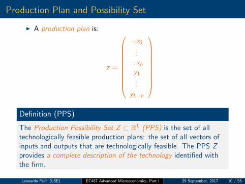
I A production plan is:

z =

−x1...−xhy1...

yL−h

Definition (PPS)

The Production Possibility Set Z ⊂ RL (PPS) is the set of alltechnologically feasible production plans: the set of all vectors ofinputs and outputs that are technologically feasible. The PPS Zprovides a complete description of the technology identified withthe firm.


One Input One Output

Example of one input x and one output y production plan

z =

(−xy

).

6

-

Z

z2 = y

z1 = x


Short-run PPS

I Sometime is possible to distinguish between:

I immediately technologically feasible production plansZ (x l , . . . , xh);

I and eventually technologically feasible production plans Z .

I Consider

Z (x1) =

z =

−x1−x2y

∣∣∣ x1 = x1

I For example if the input x1 is fixed at the level x1 then we can

define a short-run or restricted production possibility set.


Input Requirement Set and Isoquant

I A special feature of a technology is the input requirement set:

V (y) =

{x ∈ Rh

+

∣∣∣ ( −xy

)∈ Z

}

the set of all input bundles that produce at least y units ofoutput.

I We define also the isoquant to be the set:

Q(y) ={x ∈ Rh

+

∣∣∣x ∈ V (y) and x 6∈ V (y ′), ∀y ′ > y}

all input bundles that allow the firm to produce exactly y .


Two Inputs One Output

-

6x1

x2

V (y)

Q(y)

O


Production Function

Consider a technology with only one output

Definition

Production function in the case of only one output:

f (x) = supy ′

{(−xy ′

)∈ Z

}the maximal output associated with the input bundle x .


Technologically Efficient

In general, we can define the technologically efficient productionplan z as:

Definition

The general production plan z =

(−xy

)∈ Z is technologically

efficient, if and only if there does not exist a production plan

z ′ =

(−x ′y ′

)∈ Z such that z ′ ≥ z (z ′i ≥ zi ∀i) and z ′ 6= z .

If z is efficient it is not possible to produce more output with agiven input or the same output with less input (sign convention).


Example: Cobb-Douglas Technology

I We definite the Cobb-Douglas technology as

f (x1, x2) = xα1 xβ2 , α > 0, β > 0

or

Z =

−x1−x2

y

∣∣∣y ≤ xα1 xβ2

I with isoquant:

Q(y) ={

(x1, x2) ∈ R2+

∣∣∣y = xα1 xβ2

}I and input requirement set:

V (y) ={

(x1, x2) ∈ R2+

∣∣∣y ≤ xα1 xβ2

}Leonardo Felli (LSE) EC487 Advanced Microeconomics, Part I 29 September, 2017 17 / 55

Cobb-Douglas Isoquant

-

6x1

x2

V (y)

Q(y)

O


Example: Leontief Technology

I We definite the Leontief technology as

f (x1, x2) = min{ax1, bx2}, a > 0, b > 0

or

Z =

−x1−x2

y

∣∣∣y ≤ min{ax1, bx2}

I with isoquant:

Q(y) ={

(x1, x2) ∈ R2+

∣∣∣y = min{ax1, bx2}}

I and input requirement set:

V (y) ={

(x1, x2) ∈ R2+

∣∣∣y ≤ min{ax1, bx2}}

I where efficiency imposes x1 =y

a, x2 =

y

bLeonardo Felli (LSE) EC487 Advanced Microeconomics, Part I 29 September, 2017 19 / 55

Leontief Isoquants

6

-

x2

x1

x2 = ab x1

6


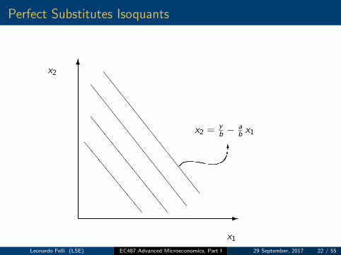
Example: Perfect Substitutes

I We definite the technology where inputs are perfectsubstitutes as

f (x1, x2) = ax1 + bx2, a > 0, b > 0

or

Z =

−x1−x2

y

∣∣∣y ≤ ax1 + bx2

I with isoquant:

Q(y) ={

(x1, x2) ∈ R2+

∣∣∣y = ax1 + bx2}

I and input requirement set:

V (y) ={

(x1, x2) ∈ R2+

∣∣∣y ≤ ax1 + bx2}


Perfect Substitutes Isoquants

6

-

\\\\\\\\\\\\\

\\\\\\\\\\\\\

\\\\\\\\\\\

eeeeeeee

x2

x1

x2 = yb −

ab x1

6


Assumptions on PPS

Common assumptions on the PPS are:

1. Z is closed (it contains its boundaries). It is an importantproperty for the definition of a production function:

sup is a max.

2. 0 ∈ Z . Shut-down property. It is an uncontroversial propertyin the long run, not necessarily in the short run (inputs usedwith no outputs).

3. Free disposal, monotonicity: if z ∈ Z and z ′ ≤ z then z ′ ∈ Z .Alternatively: if x ∈ V (y) and x ′ ≥ x then x ′ ∈ V (y).

Given a feasible production plan if either one increases thequantity of inputs or reduces the quantity of output the newproduction plan is still feasible.


Assumptions on PPS (cont’d)

4. Additivity: if z , z ′ ∈ Z then z + z ′ ∈ Z (stronger condition).For f (x) this property implies f (x1 + x2) ≥ f (x1) + f (x2).

5. Convexity of V (y): if x , x ′ ∈ V (y) then tx + (1− t)x ′ ∈ V (y)for every 0 ≤ t ≤ 1 which means that V (y) is convex set.(rescaling of production processes).

5′. A similar condition may (or may not) be imposed on the Z : ifz , z ′ ∈ Z then tz + (1− t)z ′ ∈ Z for every 0 ≤ t ≤ 1, or Z isa convex set.

Notice that the latter condition is stronger than the former.


Some Results

Result

The convexity of Z implies the convexity of V (y). The oppositeimplication does not hold.

Proof: It follows from the convexity of Z , the definition of V (y)and the following counter-example of a one-input x and one outputy technology.

-

6y

x

Z

V (x)


Some Results (cont’d)

Result

The convexity of V (y) implies that the f (x) is quasi-concave.

Proof: It follows from the convexity of V (y) and the definition ofa quasi-concave f (x).

Definition (quasi-concavity)

The function f (·) is quasi-concave if and only if the set{x | f (x) ≥ k} is convex for every k ∈ R.

Notice that if you choose y = k the set above is V (y).


Some Results (cont’d)

Result

The convexity of Z implies that f (x) is (weakly) concave.

Proof: Consider

z =

(−xf (x)

)∈ Z , z ′ =

(−x ′f (x ′)

)∈ Z

Convexity of Z implies that for every 0 ≤ t ≤ 1

t z + (1− t) z ′ =

(−(t x + (1− t) x ′)tf (x) + (1− t)f (x ′)

)∈ Z

By definition of f (x) this means:

tf (x) + (1− t)f (x ′) ≤ f (tx + (1− t)x ′)

for every 0 ≤ t ≤ 1. This is the definition of a concave f (x).


Returns to Scale

I Decreasing Returns to Scale: (DRS) if z ∈ Z then t z ∈ Z forevery 0 ≤ t ≤ 1 (graph.).

I Increasing Returns to Scale: (IRS) if z ∈ Z then t z ∈ Z forevery t ≥ 1 (graph.).

I Constant Returns to Scale: (CRS) if z ∈ Z then t z ∈ Z forevery t ≥ 0 (graph.).


More Results

Result

Assumptions 0 ∈ Z and Z convex imply DRS.

Proof: It follows from the definition of convexity applied atz ′ = 0.

Result

A technology exhibits CRS if and only if the production functionf (x) (if available) is homogeneous of degree 1.


More Results (cont’d)

Proof: Assume CRS. This implies that if z ∈ Z then t z ∈ Z , forall t ≥ 0.

By definition of Z , z ∈ Z means

y ≤ f (x)

further t z ∈ Z meanst y ≤ f (t x).

By definition of production function choose z , and hence x and y ,so that y = f (x).



We can re-write the latter condition as:

t f (x) ≤ f (t x)

We need to prove that the equality holds.

Suppose it does not. Then there exists y ′ such that

t f (x) < y ′ < f (t x)

Now y ′ < f (t x) implies by definition of Z that(−t xy ′

)∈ Z



By CRS we get

1

t

(−t xy ′

)∈ Z or

(−x1t y ′

)∈ Z

which means(1/t) y ′ ≤ f (x)

ory ′ ≤ t f (x)

the latter inequality contradicts t f (x) < y ′.

The opposite implication is an immediate consequence of thedefinition of homogeneity of degree 1.


Conditions for DRS and IRS

Weaker conditions apply for DRS and IRS technology.

Result

Consider a technology characterized by a homogenous of degreeα < 1 (α > 1) production function. This technology exhibits DRS(IRS). The opposite implication does not hold.

Result

Assume that f (0) = 0 then we can prove:

I f (x) concave implies DRS;

I f (x) convex implies IRS;

I f (x) concave and convex implies CRS.


Definitions

We can now introduce few definitions:

Definition (MP)

The marginal product of input xi is

MP =∂f (x)

∂xi

Definition (AP)

The average product of input xi is

AP =f (x)

xi


Definitions (cont’d)

Definition (MRTS)

The marginal rate of technical substitution between input xi and xjis ∣∣∣∣dxidxj

∣∣∣∣ =∂f (x)/∂xj∂f (x)/∂xi

this is the absolute value of the slope of the isoquant.

The set of output bundles that are efficient for a given technology:

Definition (PPF)

The Production Possibility Frontier:

PPF (x) =

{y∣∣∣ 6 ∃z ′ ∈ Z s.t. z ′ ≥ z =

(−xy

)}


Definitions (cont’d)

We can then define

Definition (MRT)

The Marginal Rate of Transformation between output ym and yn is

MRT =dymdyn

as the slope of the PPF.


The Competitive Firm

I Assume that input and output prices are taken parametrically(no influence on such prices).

I As you have seen in consumer theory what this means is thatwhatever each firm decides in term of production does notaffect the market.

I In other words, either firms are very small with respect to themarket.


The Competitive Firm (cont’d)

I Alternatively we are assuming that firms are not strategic:they do not realize that their choices trigger reactions in otherfirms in the market,

I or any of their potential choices would be taken into accountby competitors when making their own choices.

I We will come back to this in the second part of the coursewhere we will assume and analyze economic agents that arestrategic.


Profit Maximization

The basic producer problem is than profit maximization:

max{x ,y}

p y −h∑

i=1

wi xi

s.t.

(−xy

)∈ Z

where p and wi are taken as parameters.


Profit Maximization (cont’d)

Let:

I the h-dimensional vector of input prices be w = (w1, . . . ,wh);

I the L-h-dimensional vector of output prices bep = (p1, . . . , pL−h).

We can re-write the producer’s problem as:

max{z}

p̂ z

s.t. z ∈ Z

where p̂ = (w , p) and z =

(−xy

).



In the case of a technology that produces only one output theprofit maximization problem may be written as:

max{x ,y}

p f (x)− w x

The necessary first order conditions of this problem are:

p ∇f (x∗) ≤ w

or∂f (x∗)

∂xi≤ wi

p, ∀i = 1, . . . , h

and [∂f (x∗)

∂xi− wi

p

]x∗i = 0, ∀i = 1, . . . , h.



I In the event that the production possibility set is convex (theproduction function is concave) the first order conditions areof course both necessary and sufficient.

I In other case, the following set of sufficient conditions for alocal maximum have to be verified.

I The Hessian matrix of the production function has to benegative definite at the point x∗.



This condition can be checked by the sufficient determinantcondition according to which the leading principal minors have toalternate sign starting from the negative one.

For the case of two variables the first order conditions are fori = 1, 2:

∂f (x∗)

∂xi≤ wi

p

and [∂f (x∗)

∂xi− wi

p

]x∗i = 0



while the second order conditions are:

H =

∂2f (x∗)∂x21

∂2f (x∗)∂x1 ∂x2

∂2f (x∗)∂x1 ∂x2

∂2f (x∗)∂x22

negative definite

Which is implied by:∂2f (x∗)

∂x2i< 0

and∂2f (x∗)

∂x21

∂2f (x∗)

∂x22−(∂2f (x∗)

∂x1 ∂x2

)2

> 0


Unconditional Factor Demand and Supply Function

The solution to the profit maximization problem if it existsprovides the unconditional factor demands:

x(p,w) = x∗

By substitution it is possible to obtain the supply function of theproducer:

y(p,w) = f (x(p,w)).

Comparative statics results obtained by differentiating the FOC(they are identities in (p,w)).


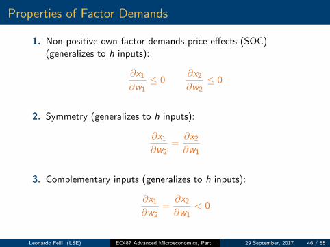
Properties of Factor Demands

1. Non-positive own factor demands price effects (SOC)(generalizes to h inputs):

∂x1∂w1

≤ 0∂x2∂w2

≤ 0

2. Symmetry (generalizes to h inputs):

∂x1∂w2

=∂x2∂w1

3. Complementary inputs (generalizes to h inputs):

∂x1∂w2

=∂x2∂w1

< 0


Properties of Factor Demands (cont’d)

4. Substitutability of inputs (it does not generalize):

∂x1∂w2

=∂x2∂w1

> 0

5. Finally positive output price effects (generalizes to h inputs):

∂x1∂p

> 0∂x2∂p

> 0

(If x1 and x2 are complementary inputs.)


Properties of Supply Function

Comparative static results obtained differentiating the supplyfunction of the firm:

y(p,w) = f (x(p,w))

6. Own price effect non-negative:

∂y

∂p≥ 0

7. Symmetry:

−∂xi∂p

=∂y

∂wi

for i = 1, 2.


Summary of the Properties

Such comparative statics properties can be summarized as:

∂y∂p

∂y∂w1

∂y∂w2

−∂x1∂p − ∂x1

∂w1− ∂x1∂w2

−∂x2∂p − ∂x2

∂w1− ∂x2∂w2

s.t.

+ a ba + cb c +


Other Properties

8. Both x(p,w) and y(p,w) are homogeneous of degree 0.

Proof: If you increase both input and output prices by afactor t > 0 you obtain:

maxx

(tp) f (x)− (tw) x = maxx

t [p f (x)− w x ]

which clearly is solved by the same vector x(p,w) thatsolves:

maxx

p f (x)− w x

Further, by definition of supply function:

y(tp, tw) = f (x(tp, tw)) = f (x(p,w)) = y(p,w)


Profit Function

Definition (Profit Function)

The following is defined as the profit function

π(p,w) = maxx

p f (x)− w x = p f (x(p,w))− w x(p,w)

Properties:

1. Price effects:∂π

∂wi≤ 0

∂π

∂p≥ 0.


Properties of the Profit Function

2. The profit function π(p,w) is homogeneous of degree 1 in(p,w).

Proof: It follows from the homogeneity of degree 0 ofx(p,w) and, for any scalar α,

π(αp, αw) = α p f (x(αp, αw))− α w x(αp, αw)

= α p f (x(p,w))− α w x(p,w)

= α [p f (x(p,w))− w x(p,w)]

= α π(p,w)


Properties of the Profit Function (cont’d)

3. Hotelling Lemma (which proves property 1):

∂π

∂p= y(p,w) ≥ 0 and

∂π

∂wi= −xi (p,w) ≤ 0

Proof: It follows by Envelope Theorem applied to

π(p,w) = maxx

p f (x)− w x = p f (x(p,w))− w x(p,w)


Properties of the Profit Function

4. The profit function π(p,w) is convex in (p,w).

Proof: Consider the two price vectors (p,w) and (p′,w ′) andfor every scalar λ ∈ (0, 1) let

p′′ = λ p + (1− λ) p′

andw ′′ = λw + (1− λ)w ′


Properties of the Profit Function (cont’d)

I Then :

π [p′′,w ′′] = p′′ f (x(p′′,w ′′))− w ′′ x(p′′,w ′′)

= λ [p f (x(p′′,w ′′))− w x(p′′,w ′′)]+ (1− λ) [p′ f (x(p′′,w ′′))− w ′ x(p′′,w ′′)]

≤ λπ(p,w) + (1− λ)π(p′,w ′)

which proves convexity of π(p,w).


ec487 advanced microeconomics, part i: lecture 1

Documents