easyscan 2 afm - usna · static force mode 97 ... spreading resistance mode 102 ... line help file...
TRANSCRIPT

Operating Instructions
easyScan 2 AFMVersion 1.6

‘NANOSURF’ AND THE NANOSURF LOGO ARE TRADEMARKS OF NANOSURF AG, REGIS-
TERED AND/OR OTHERWISE PROTECTED IN VARIOUS COUNTRIES.
© MAY 07 BY NANOSURF AG, SWITZERLAND, PROD.:BT02089, V1.6R0

Table of contents
The easyScan 2 AFM 9Features...............................................................................................10easyScan 2 Controller 10Scan Heads 12Measurement modes 13
Components of the System .................................................................15Contents of the Tool set 17
Connectors, Indicators and Controls ...................................................18The Scan head 18The Controller 18
Installing the easyScan 2 AFM 21Installing the Hardware ........................................................................22
Installing the Basic AFM Package 23Installing the AFM Video Module 24Installing the Signal Module: S 24Installing the Signal Module: A 24Turning on the Controller 24
Storing the Instrument .........................................................................25Installing the Software .........................................................................26
Step 1 - Installation of hardware drivers 27Step 2 - Installation of the easyScan 2 software 33Step 3 - Installation of DirectX 9 34Installing the software on different computers 34Installing the drivers for the AFM Video Module 34
Preparing for Measurement 36Initialising the easyScan 2 controller ...................................................36Installing the cantilever ........................................................................37
Selecting a cantilever 37Inserting the cantilever in the Scan head 38
Installing the sample ............................................................................41Preparing the Sample 41Nanosurf Samples 42Stand-alone measurements 44The sample stage 45Mounting a sample onto the sample holder 45
A First Measurement 47Running the microscope simulation.....................................................47Preparing the instrument .....................................................................48
Entering values in the control panels 48
3

TABLE OF CONTENTS
4
Approaching the sample......................................................................50Manual Coarse approach 51Manual approach using the approach stage 51Automatic final approach 52
Starting a measurement ......................................................................54Selecting a measurement area............................................................55Storing the measurement ....................................................................57Creating a report..................................................................................57Finishing ..............................................................................................58
Improving measurement quality 60Removing interfering signals ...............................................................60Judging measurement quality..............................................................61Adjusting the measurement plane .......................................................62
Measurement modes 65Static Force .........................................................................................65Dynamic Force ....................................................................................66Phase Contrast ....................................................................................67
Phase measurement 68Force Modulation.................................................................................69Spreading Resistance .........................................................................70
The Signal Modules 72Signal Module: S .................................................................................72Signal Module: A .................................................................................73
Using the User Inputs and Outputs 75
Maintenance 76Scan head 76Scan electronics 76
Problems and Solutions 77Software and Driver problems .............................................................77
No connection to microscope 77USB Port error 77Driver problems 78
AFM measurement problems ..............................................................80Probe Status light blinks red 80Image quality suddenly deteriorates 81
Nanosurf support .................................................................................81Self help 81Assistance 82
AFM Theory 83

Scanning Probe Microscopy ................................................................83The Nanosurf easyScan 2 AFM...........................................................84
The user interface 87The main window.................................................................................87Operating windows ..............................................................................88Measurement document windows .......................................................89Tool bars..............................................................................................89
Arranging tool bars 89Control panels......................................................................................90
Arranging control panels 91Storing and retrieving the workspace 91Entering values in the control panels 92Storing and retrieving measurement parameters 93
The User Interface Dialog....................................................................94
Hardware setup 95The Operating mode panel ..................................................................95
STM mode 96Static Force mode 97The User Signal Editor 98Dynamic Force mode 99Phase Contrast mode 101Force Modulation mode 102Spreading Resistance mode 102
The Z-Controller Panel ......................................................................102Cantilever types configuration ...........................................................105
The cantilever browser dialog 106The cantilever editor dialog 107
Scan head configuration ....................................................................107The scan head selector dialog 107The scan head calibration editor 108The Scan Axis Correction Dialog 110
The Controller Configuration dialog ...................................................110The Edit Access Codes Dialog ..........................................................112The Scan head Diagnosis dialog .......................................................112Simulate Microscope .........................................................................112The About dialog................................................................................113
Positioning 115The Approach panel ..........................................................................115The Video panel.................................................................................118
Imaging 120The imaging bar.................................................................................121
5

TABLE OF CONTENTS
6
The Imaging panel.............................................................................123
Spectroscopy 128The Spectroscopy bar .......................................................................129The Spectroscopy panel....................................................................130
Viewing measurement data 134Charts ................................................................................................134
Storing and retrieving the chart arrangement 135The Chart bar ...................................................................................135
The Chart properties dialog 137Changing the appearance of the 3D view 138The Color Palette dialog 139
The Data Info panel ...........................................................................140
Quick Evaluation Tools 141The Tool Results panel .....................................................................141The Tools bar ....................................................................................141
Storing measurements and further data processing 151Storing and Printing measurements ..................................................151Creating a report................................................................................153
The Report Menu 154The Report generator configuration dialog 155
Automating measurement tasks 156The Script Menu ................................................................................156The Script Editor ................................................................................157The Script Configuration Dialog.........................................................158
Quick Reference 162

7

TABLE OF CONTENTS
8
About this ManualThis manual is divided in two parts, the first part gives instructions on how to set up and use your Nanosurf easyScan 2 AFM system. The second part is a reference for the Nanosurf easyScan 2 Control Software. It applies to software version 1.6. If you are using a newer software version, try to down-load a newer version of the manual from the Nanosurf support pages, or refer to the ‘Whats new’ file that is installed in the Manuals subdirectory of the directory where the easyScan 2 software is installed.
The first part of the manual starts with the chapter Installing the easyScan 2 AFM, which should be read when installing your easyScan 2 AFM system. The chapters Preparing for Measurement and A First Measurement should be read by all users, because they contain useful instructions for everyday measurements. The other chapters give more information for advanced or interested users.
The second part of the manual starts with chapter The user interface (p.87). This part is a description of the function of the buttons and inputs in the dialogs and control panels of the easyScan Control software. Chapter Quick Reference (p.162) gives links to the description of each Control Panel, Dia-log, Menu item and Operating Window.
For more information on the optional Scripting interface, refer to the on-line help file easyScan 2 Programmers Manual, that is installed together with the easyScan 2 software.
For more information on the optional Nanosurf Report software, refer to the on-line help, included with the Nanosurf Report software.

The easyScan 2 AFM
The Nanosurf easyScan 2 AFM is an atomic force microscope system that can make nanometer scale resolution measurements of topography and sev-eral other properties of a sample. The easyScan 2 AFM system is a modular scanning probe system that can be upgraded to obtain more measurement capabilities. The main parts of the basic system are the easyScan 2 AFMscan head, the AFM Sample stage, the easyScan 2 Controller with AFM Basic module, and the easyScan 2 software. At the time of publication, the following parts can be used with the easyScan 2 system:
• STM Scan Head: makes atomic scale measurements. Refer to the easy-Scan 2 STM Operating Instructions for more details.
• AFM Dynamic Module: adds dynamic mode measurement capabilities for measuring delicate samples.
• AFM Mode Extension Module: adds phase contrast, force modulation and current measurement capabilities.
• AFM Video Module: allows observation of the approach on the computer screen. This is especially useful when observation using the lenses is impractical.
• Signal Modules: allow monitoring signals (Module: S) and creating cus-tom measurement modes (Module: A). Refer to chapter The Signal Mod-ules (p.72) for more details.
• Micrometre Translation Stage: for reproducibly finding a specific posi-tion on the sample.
• Nanosurf Report: software for simple automatic evaluation and reporting of surface measurements.
• Nanosurf Analysis: software for detailed analysis of scanning probe meas-urements.
• Scripting Interface: software for automating measurements. Refer to chapter Automating measurement tasks (p.156) and the Programmer’s Manual for more details.
9

THE EASYSCAN 2 AFM
10
• TS-150 active vibration isolation table: reduces the sensitivity of the instrument to vibrations in its environment.
Features
easyScan 2 Controller
Electronics
Control Software
Controller size / weight 470x120x80 mm / 2.4 kgPower supply 90 - 240 V~/ 30 W 50/60 HzComputer interface (Appr. controller serial number 23-06-030
and higher)Integrated USB hub 2 Ports (100mA max)Scan generator 16 bit D/A converter for all axesScan speed Up to 60ms/line at 128 datapoints/lineScan drive signals ± 10 V, no high voltageMeasurement channels 16bit A/D converters, up to seven signals
depending on mode.Scan area and data points Individual width/height, up to 2048 x 2048
pointsScan image rotation 0 - 360°Sample tilt compensation Hardware X/Y-slope compensationSpectroscopy modes Single point measurement or multiple meas-
urements along vectorSpectroscopy measurement averaging
1 - 1024 times
Spectroscopy data points Up to 2048
Simultaneous display of data in charts types
Line graph, Color map, 3D view, …
User profiles Customisable display and parameter settings

FEATURES
Nanosurf easyScan 2 Scripting Interface
Computer requirements
Computer not included with system.
Nanosurf easyScan 2 Signal Module: S
Nanosurf easyScan 2 Signal Module: A
On-line processing func-tions
Mean fit, Polynomial fit, Derived data, …
Quick evaluation functions distance, angle, cross section, roughness, …Data export BMP, ASCII, CSV, …
Applications Automating measurement tasks, lithography, custom evaluation functions, using third party measurement equipment
Included control software Windows Scripting Host: Visual Basic Script, Java Script, …
Remote control by COM compatible languages: LabView, MathLab, Visual Basic, Delphi, C++, …
Operating system require-ment
Windows 2000, XP, Vista
Electronics interface USB portRecommended PC hardware Pentium 4/M or AMD Athlon, 256MB
RAM, True color > 1024x786 video card, HW Open GL accelerator
Available output signals X-Axis, Y-Axis, Z-Axis, Approach, Tip Volt-age, STM Current or AFM Deflection, Excitation, Amplitude, Phase
Full scale corresponds to ±10 V, Excitation: ±5 VPower supply output GND, +15 V, -15 V
Output signal All output signals of Signal Module: S
Simultaneous display of data in charts types
Line graph, Color map, 3D view, …
11

THE EASYSCAN 2 AFM
12
User inputs can optionally be measured in all Imaging and Spectroscopy modes.
User outputs can be modulated in Spectroscopy measurements.
Scan Heads
1) Manufacturing tolerances are ±15 % for 10 µm and 70 µm heads, ±10 % for 110 µm scan heads. The exact values are given on the calibration certificate delivered with the instrument.
2) Calculated by dividing the maximum range by 16 bits
Scanner features
Additional analog user out-puts
2x 16 bit D/A converters, ±10 V
Synchronisation output 1x TTL: start, end, point syncAdditional signal modulation inputs
X-Axis, Y-Axis, Z-Axis, Tip Voltage, Excita-tion
Free connectors 2x Aux, connection made on user requestModulation range ±10 V, Excitation: ±5 VAdditional analog user inputs 2x 16 bit A/D converters, ±10 VAdditional modes Almost unlimited
AFM Scan Head: 10 µm 70 µm 110 µm
Maximum Scan range 1) 10 µm 70 µm 110 µm
Maximum Z-range 2 µm 14 µm 22 µm
Drive resolution Z 2) 0.027 nm 0.21 nm 0.34 nm
Drive resolution XY 2) 0.15 nm 1.1 nm 1.7 nm
XY-Linearity Mean Error <0.6% <1.2% <0.6% Z measurement noise level (RMS, Static Mode)
0.07 nm (max. 0.2 nm)
0.6 nm (max. 0.8 nm)
0.4 nm (max. 0.55 nm)
Z measurement noise level (RMS, Dynamic Mode)
0.04 nm (max. 0.07 nm)
0.5 nm (max. 0.8 nm)
0.3 nm (max. 0.55 nm)
Design Tripod stand-alone

FEATURES
Compatible cantilevers
Measurement modes
AFM Basic Module
The AFM Basic Module is required for using AFM Scan Heads.
Sample size UnlimitedAutomatic approach range 5 mmMax. approach speed 0.1 mm/sAlignment of cantilever Automatic adjustmentElectrical connection to tip AvailableScan head weight 350 gSample observation optics Dual lens system (top/side view)Optical magnification Top x12 / side x10View field Top 4x4 mm / side 5x3 mmSample illumination White LEDs sideways illumination, adjust-
able brightness
Manufacturers NanoSensors® and NanoWorld®
Applied Nanostructures
Static modes CONTR, LFMR, ZEILR SICONADynamic modes NCLR, ZEIHR, EFM,
MFMRACLA, MAGT, FORTA
Spreading Resist-ance mode
CONTPt, NCLPt, CDT-NCLR
ANSCM-PC, ANSCM-PT
Available tips Standard, SuperSharp Sili-con, HighAspectRatio, Diamond
Rotated pyramidal (stand-ard)
Typical static load 10 nN
Imaging modes Static Force (Contact): Const. Force (Topo-graphy), Const. Height (Deflection)
Spectroscopy modes Force-Distance, Force-Tip voltageTip voltage ±10 V in 5 mV steps
13

THE EASYSCAN 2 AFM
14
AFM Dynamic Module
The AFM Basic Module is required for using the AFM Dynamic Module.
AFM Mode Extension Module
Both the AFM Basic Module and the AFM Dynamic Module are required for using the AFM Mode Extension Module.
AFM Video Module
Micrometre Translation Stage
Additional imaging modes Dynamic Force (Intermittent Contact, etc.): Const. Amplitude (Topography), Const. Height (Amplitude)
Additional spectroscopy modes Amplitude-DistanceDynamic frequency range 15kHz - 300kHzDynamic frequency resolution < 0.1Hz
Additional imaging modes Phase Contrast, Force Modulation, Spread-ing Resistance
Additional spectroscopy modes
Phase-Distance, Current-Voltage, Current-Distance etc.
Phase contrast range ± 90°Phase contrast resolution < 0.05°Phase reference range 0 - 360°Tip current measurement ± 100µA, 3nA resolution
Camera system Dual video (top/side view)Magnification Top: 100x / side: 70xView field Top: 3.2x2.7 mm / side: 4.1x3.4 mmImage pixels 352x288Video display In control software, can be saved as JPEGAnalog video output PAL Video-SAdditional sample illumina-tion
Version 2 video cameras: constant axial illu-mination for top view
X-Y resolution < 0.5 µm

COMPONENTS OF THE SYSTEM
Components of the System
This section describes the parts that may be delivered with an easyScan 2 AFM system. The contents of delivery can vary from system to system, depending on which parts were ordered. To find out which parts are included in your system, refer to the delivery note shipped with your sys-tem. Some of modules listed in the delivery note are built into the Control-ler. Their presence is indicated by the status lights on the top surface of the Controller when it is turned on (section Connectors, Indicators and Controls(p.18)).
1. easyScan 2 Controller with a built in AFM Basic Module, and option-ally with built in AFM Dynamic Module, AFM Mode Extension Mod-ule, Video Module electronics and Signal Module A or S electronics
Travel 13 mm
Components: The easyScan 2 AFM system
1
7
12
32
4 5 6
18
13 17
19
15

THE EASYSCAN 2 AFM
16
2. USB cable
3. Mains cable
4. easyScan 2 AFM Scan head(s) with AFM Video Camera (with AFM Video Module)
5. Scan head case
6. Scan head cable
7. Video Camera cable (with AFM Video Module)
8. AFM calibration certificate
9. This easyScan 2 AFM Operating Instructions manual
10. easyScan 2 Software Reference manual
11. easyScan 2 Installation CD: Contains software, calibration files, and PDF files of all manuals
12. AFM Tool set (option). The contents of the AFM Tool set are described in the next section.
13. AFM Extended Sample Kit (option, not shown) with set of 10 samples and description of experiments.
14. AFM Sample Stage (option)
15. Micrometre Translation Stage (option)
16. User's Guide; Translation Stage, Model: 9064 (with Micrometre Trans-lation Stage)
17. Positioning Tool Set (with Micrometre Translation Stage)
18. Break-out cable (with Signal Module: S)
19. Connector box (with Signal Module: A)
20. Signal Module cables (2x) (with Signal Module: A)
21. Scripting Interface Certificate of purchase with Activation key printed on it (with Scripting Interface)
22. Instrument Case
The package may also contain easyScan 2 STM head(s) and modules for the STM, which are described in the STM Operating Instructions

COMPONENTS OF THE SYSTEM
Contents of the Tool setThe contents of the Tool set depends on the available modules. It may con-tain:
1. Ground cable
2. Protection feet
3. Cantilever tweezers: ACA 103
4. Screwdriver, 2.3 mm
5. Cantilever insertion tool (usually mounted in DropStop)
6. DropStop
7. Sample holder (with AFM Sample Stage)
8. a) AFM Large Scan Sample kit (option) with Grid: 10µm / 100nm, CD ROM piece b) AFM High Resolution Sample Kit (option) with Grid: 660 nm, Graphite (HOPG) sample on sample support c) AFM Basic Sample Kit (option, no longer available) with CD-ROM Sample, Microstructure sample
9. AFM Calibration Samples Kit (option) with Calibration grid: 10 µm/100nm, Calibration grid: 660nm, Flatness sample
10. Set of 10 CONTR cantilevers (option)
11. Set of 10 NCLR cantilevers (option)
Contents of the AFM Tool set
12
76
8
9 10
1 2 345
11
17

THE EASYSCAN 2 AFM
18
12. USB dongle for the Nanosurf Report software (option)
Connectors, Indicators and Controls
Use this section to find the location of the parts of the easyScan 2 AFM that are referred to in this manual.
The Scan head
The Controller
Status lightsAll status lights on top of the Controller will light up for one second when the power is turned on.
The Probe Status lightIndicates the status of the Z-Feedback loop. It can indicate the following statuses:
red The scanner is in its upper limit position. This occurs when the tip-sample interaction is stronger than the set point for some time. There is danger of damaging the tip due to too high an interaction.
Parts of the scan head: Scan head with video camera
Scan head cable connector
Levelling screws
Ground connector
Socket for Cantilever insertion tool
Cantilever on Alignment chip
Cameraconnector
Scan head serial number

CONNECTORS, INDICATORS AND CONTROLS
orange/yellow The scanner is in its lower limit position. This occurs when the tip-sample interaction is weaker than the set point for some time. The tip is probably not in contact with the sample surface.
green The scanner is not in a limit position, and the feed-back loop can measure the sample surface.
blinking green The feedback loop has been turned off in the software.
blinking red There is no signal with which to do feedback: The light intensity on the photodetector of the laser beam deflection system is too low. Refer to section Probe Status light blinks red (p.80)) for more information.
The Scan Head lightsIndicate the scan head type that is connected to the instrument. The Scan
The easyScan 2 Controller
Video Outconnector(optional)
Probe Status light
Scan head cable connector
Video Inconnector(optional)
Signal Out connector(optional)
Signal In connector(optional)
Scan Head lightsModule lights
Powerswitch
USB activelight
Mains powerconnector
USB powerlight
USB input(from PC)
ControllerSerial number
USB outputs(to dongle)
S/N: 23-05-001
19

THE EASYSCAN 2 AFM
20
head lights blink when no scan head can be detected, or when the Control-ler has not been initialised yet.
The Module lightsIndicate the modules that are built in into the Controller. The module lights blink when the Controller has not been initialised yet. During initial-isation, the Module lights are turned on one after the other.

CONNECTORS, INDICATORS AND CONTROLS
Installing the easyScan 2 AFM
The following sections describe the installation of the easyScan 2 AFM.
IMPORTANTTo make high quality measurements, the following precautions must be taken to keep equipment clean:
• Never touch the cantilever tips, the cantilevers (figure Contents of the AFM Tool set (p.17), 10, 11), or the open part of the Scan head (figure Cantilever deflection detection system (p.38)).
• Ensure that the surface to be measured is free of dust and possible resi-dues.
• Always put the Scan head it in the Scan head case during transport and storage (figure Scan head storage).
Scan head storage: Scan head stored in Scan head case
21

INSTALLING THE EASYSCAN 2 AFM
22
Installing the Hardware
WARNING
As a consequence:
• Always close the DropStop before inspecting or mounting a cantilever or the inspecting the alignment chip, especially when using optical instru-ments (magnifiers) for the inspection.
• Never remove the built-in top view and side view lenses from the lens cover.
• Never remove the lens cover from the scan head.
The built-in top view and side view lenses for observing the tip-sample approach have optical filters that block back-reflected laser radiation. This makes viewing the cantilever with the top and side view lenses safe.
Older Scan heads may contain lasers with 850 nm wavelength infrared light, and lower optical power. These lasers have laser class 1, which does not require special protection, even when viewing the laser radiation directly with optical instruments. The wavelength and laser class are indi-cated next to the serial number on the scan head.
IMPORTANT
• Ascertain that the mains connection is protected against excess voltage surges.
• Place the instrument on a stable support in a location that has a low level of building vibrations, acoustic noise, electrical fields and air currents.
LASER RADIATION (650nm)DO NOT STARE INTO THE BEAM
OR VIEW DIRECTLY WITH OPTICAL INSTRUMENTS (MAGNIFIERS)CLASS 2M LASER PRODUCT

INSTALLING THE HARDWARE
It is recommended to cover the instrument with a box to shield it from near infrared light from artificial light sources, because this light may cause noise in the cantilever deflection detection system. If the vibration isolation of your table is insufficient for your measurement purposes, an optional active vibration isolation table is available.
Installing the Basic AFM Package- Attach the Scan head cable (figure Components (p.15), 6) to the Scan head
(Components, 4) using the screwdriver (figure Contents of the AFM Tool set(p.17), 4).
- Connect the Scan head cable (Components, 6) to the Controller (Compo-nents, 1).
The scan head cable has a helix shape in order to isolate the Scan head from vibrations of the table it is standing on. Take care that it is lying loosely on the table to ensure proper operation, and avoid stretching it.
- Connect the USB cable (Components, 2) to a free USB port on your com-puter, but do not connect it to the easyScan 2 Controller yet. If you have inadvertently done this anyway, continue with section Installing the Soft-ware (p.26).
easyScan 2 AFM system: System with Sample stage, Micrometre Translation Stage, AFM Video Module and Signal module: A
23

INSTALLING THE EASYSCAN 2 AFM
24
Installing the AFM Video Module- Connect the Video Camera cable (Components, 7) to the connector on
the AFM Video Camera (Components, 4) and the Video In connector on the Controller (figure The easyScan 2 Controller (p.19)).
In case of an upgrade, both the scan head and the Controller must be sent in to your local Nanosurf distributor for mounting the Video Camera on the Scan Head and installing the Video Camera electronics in the Control-ler. After the Controller has been returned, you should install the drivers for the AFM Video Module (section Installing the drivers for the AFM Video Module (p.34)).
Installing the Signal Module: S- Connect the Break-out cable (Components, 18) to the Signal Out connec-
tor on the Controller (figure The easyScan 2 Controller).
In case of an upgrade, the Controller must be sent in to your local Nanosurfdistributor for mounting the Signal Module: S electronics in the Controller.
Installing the Signal Module: A- Connect one Signal Module cable (Components, 20) to the Signal Out
connector on the Controller and to the Output connector on the Signal Module: A.
- Connect the other Signal Module cable to the Signal In connector on the Controller and to the Input connector on the Signal Module: A.
In case of an upgrade, the Controller must be sent in to your local Nanosurfdistributor for mounting the Signal Module: A electronics in the Control-ler.
Turning on the Controller- Connect the easyScan 2 Controller (Components, 1) to the mains using
the mains cable (Components, 3) and turn it on.

STORING THE INSTRUMENT
First all status lights on top of the Controller briefly light up. Then the Scan Head lights and the lights of the detected modules will start blinking, and all other status lights turn off. The status lights remain blinking until the Controller is initialised by starting the easyScan 2 software.
Storing the Instrument
If you have to send in the instrument, transport it or if you are not using it for some time, please pack it in the shipping package or instrument case.
- Turn off the instrument as described in section Finishing (p.58), and remove all cables.
- Pack all components as shown in figure Packing.
Packing: The easyScan 2 AFM system packed in the Instrument Case
25

INSTALLING THE EASYSCAN 2 AFM
26
IMPORTANTBefore transport, put the Scan head in the Scan head case. Put the instru-ment in the original Nanosurf shipping package or instrument case.
Installing the Software
- Check that the computer on which you want to install the software fulfils the requirements listed in section Computer requirements (p.11).
- Disconnect the USB cable from the easyScan 2 controller.
- If you are running Windows Vista, disconnect the computer from the internet.
This way, Windows Vista can not automatically look for the most (un)suit-able driver on the Internet.
- Turn on the computer and start Windows.
IMPORTANT
• Log on to your computer as an administrator.
• Do not run any other program when you are installing the scan software.
- Insert the easyScan 2 Installation CD into the CD drive of the computer.
The setup program should start automatically. If this does not happen, pro-ceed as follows:
- Open the easyScan 2 Installation CD.
- Start the program ‘StartCDMenu.exe’.
Now continue the normal installation procedure.
- Click the ‘Full Installation of Nanosurf easyScan 2’ button.
The installation program will now start installing all components of the Nanosurf easyScan 2 AFM: The hardware drivers, the easyScan 2 software and DirectX 9.

INSTALLING THE SOFTWARE
In Windows Vista, a Dialog is displayed with the title “An unidentified program wants access to your computer”.
- Click the ‘Allow’-button.
- Follow the instructions given by the setup program.
Step 1 - Installation of hardware driversThe Nanosurf hardware needs instrument drivers for the USB hub, the USB interface and the Video Frame grabber in the video module for the easyScan 2 AFM. These drivers are installed first.
Connecting the controller to the computer
- Turn on the controller
If you do not turn on the controller, the driver for the Video module 2 will not be installed.
- Connect the USB cable to the easyScan 2 controller.
The red USB power light on the controller now lights up on controllers with normal speed USB (1.1). The red USB power light on the controller starts to blink on controllers with high speed USB (2.0).
If you have connected a high speed USB controller to a normal speed USB connector, the computer will display a message that you have connected a normal speed device to a high speed connection.
- Install the system a computer with high speed USB support if this mes-sage is displayed and you are using the video module version 2.
The image resolution of the video image will be greatly reduced if you do not use video module version 2 with a high speed USB connection.
Installing the drivers (Windows Vista)When the controller is connected to the computer, windows automatically detects that new devices have been connected to it. On some computers, the detection process takes some time (20 seconds or more), please be patient.
27

INSTALLING THE EASYSCAN 2 AFM
28
If you have already installed the control software for a Nanosurf Scanning Probe Microscope on this computer, it is possible that nothing will happen, because the drivers are installed already. If this is the case, click OK in the Step 1 Dialog.
Once the computer has detected the new devices, it will display the ‘Found New Hardware’ Dialog.
- Click on the text ‘Found New Hardware’ in the Windows task bar if the ‘Found New Hardware’ dialog is not displayed.
The ‘Found New Hardware ‘dialog, asks you when to install the drivers for all the new devices that if found:
- Select the entry ‘Locate and install driver software (recommended)’.
The ‘Windows needs your permission to continue.’ Dialog is now dis-played.
- Click the ‘Continue’-button
The following devices can be installed, depending on the configuration of your controller:
• USB <-> serial interface
• USB Serial Port
• Unknown device (Video Module)
- Look up and carry out the installation instructions for each of these devices given in the sections below.
If something went wrong during driver installation, continue the setup nor-mally. When the setup is finished, refer to section Driver problems (p.66).
- Click OK in the ‘Step 1’ dialog.
USB <-> serial interface
When the operating system finds the ‘USB <-> serial interface’, it asks what to do:
- Click the ‘Next’ button or the default choice in all other dialogs.
The driver ‘USB High Speed Serial Converter’ is now installed.

INSTALLING THE SOFTWARE
USB Serial Port
After the High Speed Serial Converter is installed, the operating system finds the ‘USB Serial Port’, it asks what to do:
- Click the ‘Next’ button or the default choice in all other dialogs.
Click the default choice in all other dialogs.The USB Serial Port is now installed.
Unknown device (Video Module)
The USB Video Adapter driver is only installed if the Controller contains a Video Module. The installation procedure depends on the version of the video module.
Video Module version 1:
When the operating system finds an ‘Unknown Device’, it asks what to do to:
- Select 'Browse my computer for driver software (advanced)'
A dialog called ‘Browse for driver software on your computer’ now opens.
- Select the path of the installation CD (usually ‘D\’).
- Check the box ‘Include subfolders’.
Windows Security will show the dialog box ‘Windows can’t verify the pub-lisher of this driver software’.
- Select ‘Install this driver software anyway’.
Windows will not install the driver, and notify that the ‘USB Video Adapter’ device has been successfully installed.
IMPORTANTRepeat Step 1 for all USB ports of the PC, in order to ensure that the USB Video Adapter works when connecting the Controller to a different PC USB port.
Video Module version 2:
When the operating system finds an ‘Unknown Device’, it asks what to do:
- Select 'Browse my computer for driver software (advanced)'
29

INSTALLING THE EASYSCAN 2 AFM
30
A dialog called ‘Browse for driver software on your computer’ now opens.
- Select the path of the installation CD (usually ‘D\’).
- Check the box ‘Include subfolders’.
The installation of the driver will now be finished. After all drivers have been installed, Found New Hardware may notify you that one ‘Device driver software was not successfully installed’. This is not a problem, it will be remedied by the next step of the installation, step 1A. This step com-pletes the installation of the Video Module version 2.
- Click the ‘OK’ button.
When the installation of the Video Module version 2 is completed, the computer must reboot. After rebooting, the drivers ‘USB Compound device’, ‘USB 2.’ A/V Converter’ and ‘USB EMP Audio device’ will be installed.
Once the computer has rebooted:
- Start the Setup program again (by double-clicking the installation CD in windows Explorer)
- Click the ‘Full Installation of Nanosurf easyScan 2’ button.
The installation procedure should now continue with STEP 2. If the instal-lation procedure does not continue, perhaps you have not waited for the message ‘ready to use’, or something else went wrong during the installation of the drivers for the video module.
Installing the drivers (Windows XP, 2000)When the controller is connected to the computer, windows automatically detects that new devices have been connected to it. On some computers, the detection process takes some time (20 seconds or more), please be patient.
If you have already installed the control software for a Nanosurf Scanning Probe Microscope on this computer, it is possible that nothing will happen, because the drivers are installed already. If this is the case, click OK in the Step 1 Dialog.

INSTALLING THE SOFTWARE
Once the computer has detected the new devices, it will display the Dialog ‘Found New Hardware’.
The following devices can be installed, depending on the configuration of your controller:
• Standard-USB-hub
• USB <-> serial interface
• USB Serial Port
• USB Device (Video Module)
- Look up and carry out the installation instructions for each of these devices given in the sections below.
If something went wrong during driver installation, continue the setup nor-mally. When the setup is finished, refer to section Driver problems (p.66).
- Click OK in the ‘Step 1’ dialog.
Standard-USB-hub
The operating system should first find the ‘Standard-USB-hub’, and install its driver. The installation order of the other drivers may vary.
USB <-> serial interface
When the operating system finds the ‘USB <-> serial interface’, it asks what to do:
- Select 'No not this time'
- Click ‘Next’
- Select ‘Install the software automatically (Recommended)’
- Click ‘Next’
The message ‘Installed USB <-> Serial’ is not displayed
- Click ‘Finish’
The driver ‘USB High Speed Serial Converter’ is now installed.
31

INSTALLING THE EASYSCAN 2 AFM
32
USB Serial Port
After the High Speed Serial Converter is installed, the operating system finds the ‘USB Serial Port’, it asks what to do:
- Select 'No not this time'
- Click ‘Next’
- Select ‘Install the software automatically (Recommended)’
- Click ‘Next’
The message ‘Installed USB <-> Serial’ is not displayed
- Click ‘Finish’
The driver ‘USB Serial Port’ is now installed.
USB Device (USB Video Adapter)
The USB Video Adapter driver is only installed if the Controller contains a Video Module. The installation procedure depends on the version of the video module.
Video Module version 1:
When the operating system finds the ‘USB Device’, it asks what to do to install the ‘USB Video Adapter’:
- Select 'No not this time'
- Install the software automatically (Recommended)
During installation of the video adapter under windows XP, windows may notify you that the driver is not digitally signed. If this happens:
- Click ‘Continue installation’.
- Click the default choice in all other dialogs.
IMPORTANTRepeat Step 1 for all USB ports of the PC, in order to ensure that the USB Video Adapter works when connecting the Controller to a different PC USB port.

INSTALLING THE SOFTWARE
Video Module version 2:
- Select 'No not this time'
- Click ‘Next’.
- Select 'Install the software automatically (Recommended)’
- Click ‘Next’.
The message ‘Installed USB 2.0 A/V Converter is now displayed
- Click the ‘Finish’ button.
After the installation of the Drivers has finished, a step 1A may follow, that completes the installation of the Video Module version 2.
- Click the ‘OK’ button.
When the installation of the Video Module version 2 is completed, the computer must reboot. After rebooting, windows shows the notifications:
• Found New Hardware USB Device
• Found New Hardware USB EMP Audio Device
• Your New Hardware is now ready to use.
- Wait until the ‘ready to use’ message is displayed
The drivers ‘USB Compound device’, ‘USB 2.0 A/V Converter’ and ‘USB EMP Audio device’ are now installed.
- Start the Setup program again (by double-clicking the installation CD in windows Explorer)
- Click the ‘Full Installation of Nanosurf easyScan 2’ button.
The installation procedure should now continue with STEP 2. If the instal-lation procedure does not continue, perhaps you have not waited for the message ‘ready to use’, or something else went wrong during the installation of the drivers for the video module.
Step 2 - Installation of the easyScan 2 software- Click the default choice in all dialogs.
33

INSTALLING THE EASYSCAN 2 AFM
34
The setup program will ask for the directory in which the easyScan 2 soft-ware is to be installed.
- Install the software in the proposed directory.
IMPORTANTThe easyScan 2 Installation CD contains calibration information (.hed files) specific to your instrument, therefore you should keep (a backup copy of ) the CD delivered with the instrument.
Step 3 - Installation of DirectX 9The easyScan 2 software needs DirectX 9 or newer for correct operation.
Click the default choice in all dialogs.
- After installing DirectX 9, the computer may have to re-boot.
Installing the software on different computersYou can install the easyScan 2 software on a different computer than the one that controls the measurement, for example for running the microscope simulation, or for off-line data analysis. Please note:
• In order to use the Controller, the hardware drivers and DirectX 9 must be installed on the computer to which it is connected.
• The controller and its drivers must be installed when installing the Nano-surf Scripting Interface.
Installing the drivers for the AFM Video ModuleWhen the AFM Video Module is added to your Controller after you have installed the software, its drivers must be installed before it can be used:
- Disconnect the USB cable from the Controller.
- Turn on your computer and start Windows.
IMPORTANTMake sure you have administrator privileges before software installation.

INSTALLING THE SOFTWARE
- Insert the easyScan 2 Installation CD into the CD drive of the computer.
- If the setup program has started automatically, click ‘Exit’.
- Connect the USB cable to the easyScan 2 Controller.
The red USB power light on the Controller should now light up, and the PC should now automatically detect the ‘USB Device’, and asks what to do to install the ‘USB Video Adapter’. On some computers, the detection and installation process may take some time (20 seconds or more), please be patient.
- Select ‘Automatic installation’.
During installation of the video adapter under windows XP, windows may notify you that the driver is not digitally signed. If this happens:
- Click ‘Continue installation’.
- Click the default choice in all other dialogs.
IMPORTANTConnect the USB cable to all USB ports of the PC, in order to ensure that the instrument works when connecting the Controller to a different PC USB port.
35

PREPARING FOR MEASUREMENT
36
Preparing for Measurement
This chapter describes actions that you perform on a day-to-day basis as a preparation for your measurements, when the instrument has already been set up according to the instructions in chapter Installing the easyScan 2 AFM(p.21). These steps are changing the cantilever, selecting a sample stage, and preparing the sample.
Initialising the easyScan 2 controller
- Check that the easyScan 2 controller is connected to the mains power, and the USB port of the control computer.
- Turn on the power.
First all status lights on top of the controller briefly light up. Then the Scan Head lights and the lights of the detected modules will start blinking, and all other status lights turn off.
- Start the easyScan 2 software on the control computer.
The main program window appears, and all status lights are turned off. Now a Message ‘Controller Startup in progress’ is displayed on the compu-ter screen, and the module lights are turned on one after the other. When initialisation is completed, a Message ‘Starting System’ is shortly displayed on the computer screen and the Probe Status light, Scan Head status light of the detected scan head and modules will light up. If no scan head is detected, both scan head status lights blink.
- Determine which operating mode you wish to use.
Refer to the sections on Operating modes in this manual for the properties of the various operating modes.
To change the operating mode:
- Click in the Navigator to open the Operating mode panel.
- Select the operating mode using the Operating mode drop-down menu.

INSTALLING THE CANTILEVER
Installing the cantilever
To maximise ease of use, the Nanosurf easyScan 2 AFM is designed so that the cantilever can be installed and removed without having to readjust the cantilever deflection detection system. This is possible because an align-ment system is used that consists of an alignment chip and matching grooves in the back side of the cantilever chip. This positions the cantilever with micrometer accuracy (see figure Cantilever, left). Note though, that
this accuracy is only guaranteed when the cantilever and the mounting chip are absolutely clean. Installation of the cantilever should therefore still be carried out with great care because good results depend strongly on the accuracy of this process.
Selecting a cantileverNow select the proper cantilever type for the measurement mode you wish to use. The stiffer, short NCLR cantilever is generally used for the dynamic
Cantilever: left: alignment system, centre: Cantilever chip viewed from the top, right cantilever 450 µm long, 50 µm wide with integrated tip.
37

PREPARING FOR MEASUREMENT
operating mode; the more flexible, long CONTR cantilever is generally used for the static operating mode.
When you change to a different cantilever type:
- Select the cantilever type using the ‘Mounted cantilever’ drop-down menu in the Operating mode panel.
Presently, only cantilevers from the companies NanoWorld and NanoSen-sors can be used. The various usable types are listed in section Compatible cantilevers (p.13).
Inserting the cantilever in the Scan headWARNING
As a consequence:
• Always close the DropStop before inspecting or mounting a cantilever or the inspecting the alignment chip, especially when using optical instru-ments (magnifiers) for the inspection.
• Never remove the built-in top view and side view lenses from the lens cover.
• Never remove the lens cover from the scan head.
Cantilever deflection detection system
Sample illumination
Photodetector Laser
Cantilever holder spring
Cantilever
Alignment chip
Hole for cantilever insertion tool
LASER RADIATION (650nm)DO NOT STARE INTO THE BEAM
OR VIEW DIRECTLY WITH OPTICAL INSTRUMENTS (MAGNIFIERS)CLASS 2M LASER PRODUCT
38

INSTALLING THE CANTILEVER
The built-in top view and side view lenses for observing the tip-sample approach have optical filters that block back-reflected laser radiation. This makes viewing the cantilever with the top and side view lenses safe.
Older Scan heads may contain lasers with 850 nm wavelength infrared light, and lower optical power. These lasers have laser class 1, which does not require special protection, even when viewing the laser radiation directly with optical instruments. The wavelength and laser class are indi-cated next to the serial number on the scan head.
CAUTION
• Nothing should ever touch the cantilever, especially the tip end!
• The Cantilever Holder Spring (see figure Cantilever deflection detection system) is very delicate and should not be bent!
• Always close the DropStop before handling the cantilever. Otherwise, the cantilever may fall into the scan head. This may cause malfunction of the microscope, particularly the scanner.
• If a cantilever has dropped into the scan head, and the microscope is mal-functioning, contact your local support. Never open the scan head, because this is likely to cause damage to the scanner and the laser beam deflection detection system.
To insert the cantilever:
- Remove the Cantilever Insertion tool from the DropStop
- Turn the scan-head upside-down.
- Close the DropStop (figure Closing the DropStop).
Closing the DropStop
39

PREPARING FOR MEASUREMENT
40
easyScan 2 controllerThe laser beam is now blocked by the DropStop. As a consequence, the Probe Status light on the easyScan 2 controller will now blink red.
- Place the cantilever insertion tool (figure Contents of the AFM Tool set(p.17), 5) into the hole behind the alignment chip (figure Mounting the cantilever, top left). The Cantilever Holder Spring opens.
- Use the Cantilever tweezers to remove the old cantilever from the instru-ment (figure Mounting the cantilever, top right).
It is recommended to always store the Scan head with a cantilever installed.
- Take the new cantilever out of its box. The cantilever is now oriented face up.
Mounting the cantilever: top left: Inserting the cantilever insertion tool; top right: Inserting/Removing the cantilever; bottom right: Correctly inserted cantilever

INSTALLING THE SAMPLE
- Let the cantilever carefully fit into the alignment chip in the Scan head (figure Mounting the cantilever, top right).
- Verify that the cantilever does not move with respect to the alignment chip when lightly tapping it with the tweezers.
If the cantilever does move, it is probably not inserted correctly. Refer to figure Cantilever Alignment for the correct alignment and examples of incorrect alignment.
- Gently pull the cantilever insertion tool out of the hole; the cantilever holder spring closes and holds the cantilever chip tightly in position (fig-ure Mounting the cantilever, bottom right).
- Remove the DropStop.
easyScan 2 controllerThe laser beam is now unblocked, and the Probe Sta-tus light on the easyScan 2 controller should now stop blinking red. If this is not the case refer to Chapter Problems and Solutions (p.77).
Installing the sample
Preparing the SampleThe easyScan 2 AFM can be used to examine any material with a surface roughness that does not exceed the height range of the scanning tip. Nev-ertheless the choice and preparation of the surface can influence the surface-tip interaction. Examples of influencing factors are excess moisture, dust, grease etc. Because of this some of the samples need special preparation to clean their surface. Generally, clean as little as possible.
Cantilever Alignment: left: Correct, the mirrored environment light shows a pattern that is continuous on the cantilever and the alignment chip; centre, right: Incorrect, the mirrored environment light shows a different pattern on the cantilever than on the alignment chip.
41

PREPARING FOR MEASUREMENT
42
If the surface is dusty, try to measure on a clean area between the dust. It is possible to blow coarse particles away with dry, oil free air, but small parti-cles generally stick so well to the surface that they can not be removed. Note that bottled pressurised air is generally dry, but pressurised air from an in-house supply is generally not. In this case an oil filter should be installed. Blowing dust away by breath is not advisable, because it is not dry.
When the surface is contaminated with grease, oil or something else, the surface should be cleaned with a solvent. Suitable solvents are distilled or demineralised water, alcohol or acetone, depending on the contaminant. The solvent should be very pure, in order to prevent the collection of impu-rities on the surface when the solvent evaporates. The sample should be cleaned several times to remove dissolved and redeposited contaminants if it is very contaminated. Delicate samples can be cleaned in an ultrasound bath.
Nanosurf SamplesNanosurf delivers various optional samples that are usually packed in the AFM Tool kit. These samples are described here. The description of the AFM Extended Sample kit is included in the Extended Sample kit.
All samples should be kept in their box. Then it should be unnecessary to clean them. Cleaning is not advisable, because the grids is rather delicate.
Grid: 10 µm / 100 nm
The Grid: 10 µm/100 nm can be used for testing the xy-calibration of the 70 µm and 100 µm scanners and for testing z-calibration. It is manufac-tured using a standard silicon process that produces silicon oxide squares on
Structure of Grid: 10 µm / 100 nm
100 nm
10 µm

INSTALLING THE SAMPLE
a silicon substrate. It has a period of 10 µm and a square height of approx-imately 100 nm.
size: 5 mm x 5 mm
material: silicon oxide on silicon
structure: square array of square hills of silicon oxide hills on silicon
Grid period: 10 µm, approx. height: 100 nm, calibrated values of period and height (with 3 % accuracy) given on package. Certified Calibration grids are available as an option.
Grid: 660nm
The Grid: 660 nm can be used for testing the xy-calibration of the 10 µm scanner. Depending on its make, it consists either of
• silicon oxide hills on a silicon substrate with a period of 660 nm and an unspecified height. The approximated height is 149 nm,
• holes in a silicon oxide layer with a period of 660 nm and an unspecified depth. At the time of writing, the approximated depth is 60 nm.
size: 5 mm x 5 mm
material: silicon oxide on silicon
structure: square array of holes or hills in the silicon oxide layer
period: 660 nm, calibrated value of period (with 3 % accuracy) given on package. Certified Calibration grids are available as an option.
Flatness SampleThe Flatness sample is a polished silicon sample. It can be used for testing the Flatness of the scanned plane.
Structure of Grid: 660nm (version with holes)
660 nm
60 nm
43

PREPARING FOR MEASUREMENT
44
size: 5 mm x 5 mm
material: silicon
thickness: appr. 320 µm
CD-ROM pieceSample for demonstrating the AFM imaging. The CD sample is a piece from a CD, without any coating applied to it.
material: Polycarbonate
structure: 100 nm deep pits, arranged in tracks spaces 1.6 µm apart.
MicrostructureSample for demonstrating the AFM imaging (no longer available). The microstructure is approximately the negative of the Grid: 10µm / 100nm. It consists of holes in a silicon oxide layer with an unspecified period and depth. The approximate period is 10 µm, the approximate depth is 100 nm.
Graphite (HOPG) on sample supportThe sample can be used for both STM and AFM measurements. In high resolution AFM measurements the atomic steps on the graphite surface can be seen. Conductivity variations can be observed in spreading resistance mode.
size: approx. 5 mm x 5 mm
material: Highly Oriented Pyrolytic Graphite (HOPG)
Sample support: Magnetic Steel disc, galvanically coated with Nickel.
Stand-alone measurementsYou can either use the instrument with the sample stage, or as a stand-alone instrument. The sample stage offers vibration isolation, and a stable scan head mount. Therefore, operate the instrument as a stand-alone only when the sample is too large for the sample stage. For stand-alone measurements, put the Scan head directly on top of the sample. Protection feet for under the three alignment screws are provided to protect delicate samples from being scratched (figure Contents of the AFM Tool set (p.17), 2).

INSTALLING THE SAMPLE
The sample stageThe sample stage (figure Components (p.15), 14) offers vibration isolation and stable positioning and can be used to comfortably position the sample. An optional micrometre translation stage for X-Y positioning can be mounted on the sample stage. You can either put the sample directly on the sample stage, or mount it on the sample holder (figure Contents of the AFM Tool set (p.17), 7).
Mounting a sample onto the sample holderThe simplest way to mount the sample onto the sample holder:
- Put a double-sided adhesive tape on backside of a Post-it® note, so that it is on the opposite side of the sticky side.
- Cut off the all parts of the note that do not have adhesive tape on it.
- Fix side of the note with the double-sided adhesive tape to the sample holder.
- Put the sample on the sticky side of the Post-it® note, and slightly press on it.
easyScan 2 AFM Scan head on the Sample Stage
45

PREPARING FOR MEASUREMENT
46
It is recommended to always connect the sample holder to the ground con-nector on the scan head using the ground cable (figure Contents of the AFM Tool set (p.17), 1).
CAUTIONAvoid touching the cantilever when placing the sample holder under the Scan head. If the sample touches the tip it will be damaged.
Sample mounted onto the sample holder

RUNNING THE MICROSCOPE SIMULATION
A First Measurement
In this chapter, step by step instructions are given as to how to operate the microscope and make a simple measurement. More detailed explanations of the software and the system are given in further chapters of this manual.
Running the microscope simulation
You can start the easyScan 2 software without having the microscope con-nected to your computer in order to explore the easyScan 2 system (meas-urements and software) without danger of damaging the instrument or the cantilever. In the simulation mode, most functions of the real microscope are emulated. The sample is replaced by a mathematical description of a surface.
When you start the easyScan 2 software when no microscope is connected to your PC, the following dialog appears:
- Click ‘OK’.
The status bar will now display the text ‘Simulation’.
You can also switch to the simulation mode with the microscope connected:
- Select the menu entry ‘Options>Simulate Microscope’.
A check will now be displayed in front of the menu entry.
To exit the Microscope simulation mode:
- Select the menu entry ‘Options>Simulate Microscope’ again.
The check in front of the menu entry is now removed, and the status bar will now display the text ‘Online’.
47

A FIRST MEASUREMENT
48
Preparing the instrument
IMPORTANT
• Never touch the cantilever or the surface of the sample! Good results rely heavily on a correct treatment of the tip and the sample.
• Avoid exposing the system to direct light while measuring. This could influence the beam deflection detector and reduce the quality of the measurement.
Prepare the instrument as follows (see chapter Preparing for Measurement(p.36) for more detailed instructions):
- If you have the AFM Dynamic Module, install an NCLR type cantilever, otherwise install an CONTR type cantilever.
- Install one of the samples from the Nanosurf AFM Basic sample kit or Calibration sample kit. Preferably install the 10 µm Calibration grid when using a 70µm or 110µm scan head and the 660 nm Calibration grid when using a 10µm scan head.
The measurement examples shown here were made with the 10 µm Cali-bration grid.
To make sure that the configuration is correct, do the following:
- Open the User interface dialog via the menu ‘Options/Config User Inter-face...’.
- Select the ‘Easy level’ user interface mode.
- Open the menu item ‘File>Parameters>Load...’, and load the file ‘Default_EZ2-AFM.par’ from the directory with default easyScan 2 con-figurations. Usually this is ‘C:\Program Files\Nanosurf\Nansurf easyScan 2 software\Config’.
Entering values in the control panelsTo change a parameter in any panel, use on of the following methods:
• Activate the parameter by clicking it with the mouse pointer, or by select-

PREPARING THE INSTRUMENT
ing it with the Tab key.
• The value of an activated parameter can be increased and decreased using the up and down arrow keys on the keyboard. The new value is automat-ically used after one second.
• The value of a numerical parameter can also be increased and decreased by clicking the arrow buttons with the mouse pointer. The new value is automatically used after one second.
• The value of an active numerical parameter can also be entered using the keyboard. The entered value is used on pressing the ‘Enter’ or ‘Return’ key, or by activating another input. The entered value is discarded on pressing the ‘Esc’ key. Type the corresponding character to change the unit prefix:
For example, if the basic unit is Volts, type ‘m’ to change to millivolts, type the space bar for volts, type ‘u’ for microvolts.
• The selection of a drop-down menu (e.g.: ) can be changed using the mouse or the up and down arrow keys on the key-board.
Sometimes the program will change an entered parameter value to a slightly different value. This happens when the desired value is outside the range that the easyScan 2 Controller can handle, for example due to the resolu-tion limits or timing limits. The desired value is automatically changed to the nearest possible value.
prefix keyboard key prefix keyboard keyfemto f no prefix space barpico p kilo knano n mega shift - Mmicro u giga shift - Gmilli m tera shift - T
Unit prefixes with corresponding character
49

A FIRST MEASUREMENT
50
Approaching the sample
To start measuring, the tip must come within a fraction of a nanometer of the sample without touching it with too much force. To achieve this, a very careful and sensitive approach of the cantilever is required. This delicate operation is carried out in three steps: Manual coarse approach, manual approach using the approach stage, and the automatic final approach. The colour of the probe status light on the controller shows the status of the approach:
orange Normal state during approach, the Z-scanner is fully extended toward the sample.
red The approach has gone too far, the tip was driven into the sample, and the Z-scanner is fully retracted from the sample. In this case, the tip is probably damaged, so you will have to start over again with installing a new tip.
green The approach is finished, the Z-scanner is within the measuring range.
The approach is operated using the Positioning window. To open this win-dow:
- Click the Positioning icon in the Navigator.
Use the side view of the cantilever to judge the distance between tip and the sample surface. To use the side view:
- If the AFM Video Module is installed, click in the Video panel of the Positioning window.
- If you do not have the Video Module, use the side view lens to observe the sample instead.
Even if you do not have the Video Module, you can use the Top and Side view switches to quickly change the illumination to a predetermined level.

APPROACHING THE SAMPLE
The side view should look like figure Side view of the cantilever after manual coarse approach. You can use the cantilever as a ruler to judge distances in the views of the integrated optics.
Manual Coarse approachIn this step, the sample surface is brought within the range of the fine approach stage.
- Use the three levelling screws (figure Parts of the scan head (p.18)) to lower the Scan head so that the cantilever is within 1-2 mm of the sample. Take care that the Scan head remains levelled parallel to the sample surface by turning all screws approximately the same amount.
When the sample is reflective, the mirror image of the cantilever should now be visible (figure Side view of the cantilever after manual coarse approach). When the sample is not reflective, the shadow of the cantilever may be visible. If neither a mirror image nor a shadow are visible, change the light until it is visible, for example by adding a light source, or by shad-ing the light from outside or from bright surfaces in the room.
Manual approach using the approach stageIn this step, the tip is brought as close to the sample surface as possible, without running a risk of touching it. The closer the tip is, the less time the automatic final approach takes.
- Observe the distance between tip and sample in the side view of the inte-
Side view of the cantilever after manual coarse approach
51

A FIRST MEASUREMENT
52
grated optics. The tip should not come closer to the sample than a few times the cantilever width. (figure View of the cantilever after manual approach, left).
- Whilst observing the tip sample distance, click and hold until the tip is close enough to the sample.
The sample should now be in focus. Now use the top view image to find a suitable location to measure on. In the top view, the sample is seen from a direction perpendicular to its surface (figure View of the cantilever after man-ual approach, right). To use the top view:
- If the Video Module is installed, click in the Video panel.
- If you do not have the Video Module, use the top view lens to observe the sample instead.
If necessary, move the sample holder to find a suitable location that is free of dust particles.
Automatic final approachIn the last step, the tip approaches the sample until the set point is reached.
First check that you are using the right operating mode and cantilever:
- Click in the navigator to open the Operating Mode panel.
View of the cantilever after manual approach: left: side view, right: top view

APPROACHING THE SAMPLE
- If you are operating in Static Force mode, select a CONTR type canti-lever.
In dynamic mode, the instrument will automatically determine the vibra-tion frequency used in the dynamic mode. To do this, it uses a measurement of the cantilever vibration amplitude as a function of excitation frequency. This measurement is not displayed when using the default settings. Never-theless, it is instructive to see this measurement at least once. To display the measurement:
- Open the User interface dialog via the menu ‘Options/Config User Inter-face...’.
- Select the ‘Standard level’ user interface mode.
- Enable ‘Display sweep chart’ in the Mode Properties section of the Oper-ating mode panel.
- Click the ‘Set’ button.
The software will now perform a coarse and fine frequency sweep, and dis-play the results (figure Fine frequency sweep). For more details on the fre-quency search procedure see section The Operating mode panel (p.95).
Now restore the default settings:
- Disable ‘Display sweep chart’ in the Mode Properties section of the Oper-ating mode panel.
- Select the ‘Easy level’ user interface mode.
Fine frequency sweep: Cantilever vibration amplitude as a function of frequency.
53

A FIRST MEASUREMENT
54
Now check that the set point and the feedback speed are set properly:
- Click in the Navigator to open the Z-Controller panel.
For Dynamic Force mode:
- Set ‘Set point’ to 50-70%.
For Static Force mode:
- Set ‘Set point’ to 10-20nN.
- Set ‘Loop gain’ to 1000-1500.
Now you can start the approach:
- Click in the Approach panel.
The cantilever is moved towards the sample using the approach stage, with the Z-Controller turned on. The motion continues until the Z-Controller error becomes zero. From now on the distance between sample and tip is controlled automatically by the electronics. A message ‘Approach done’ appears when the approach has been completed.
Starting a measurement
Now that the tip-sample interaction defined by Set point is flowing between tip and sample you can start measuring:
- Click to open the Imaging window.
The instrument was set to automatically start measuring after the automatic approach. Two representations of the ongoing measurement are drawn in the Imaging panel. One representation is a color coded height image, called a Color map, the other is a plot of height as a function of X* position called a Line graph. Watch the displays for a while until about a quarter of the measurement has been measured. With the current setting, the software automatically adjusts the contrast of the Color map, and height range of the Line graph to the data that have been measured.

SELECTING A MEASUREMENT AREA
ReminderMeasurements on the micrometer/nanometer scale are very sensitive. Direct light, fast movements causing air flow and temperature variations near the Scan head can influence and disturb the measurement.
When the measurement contains large disturbances, or no two scan lines are similar, stop measuring and reduce or eliminate the disturbances:
- Click and follow the instructions of the chapter Problems and Solu-tions (p.77).
Selecting a measurement area
You have prepared your measurement so that the scan line in the centre of the Line graph reproduces stably. After the measurement has been com-pleted, the color map graph should look similar to the one shown below.
Now zoom into an interesting part of the measurement:
- Activate the color map graph by clicking on it.
- Click in the imaging toolbar. The mouse pointer becomes pen- shaped when moving over the color map, and the Tool Results panel is
Zooming in on an overview measurement
55

A FIRST MEASUREMENT
56
displayed.
Select an interesting region by drawing a square with the mouse pointer:
- Click on one corner of the region using the left mouse button, and keep the button pressed.
- Drag the mouse to the other corner of the region, and then release it.
The size and the position of the square are shown in the Tool result panel.
- Release the mouse button when the square’s size covers approximately one period of the grid.
- Confirm the selection by double clicking the color map graph using the left mouse button. Now the selection is enlarged to the whole display size. You can abort the zoom function by clicking again.
The microscope will now start measuring a single grid period. Once the measurement is completed, you should get an image such as the one in figure Zoomed measurement, left. The depression in the sample surface to the sides of the structure is due to data filter used. To remove it, select the
data filter ‘Raw Data’ in the Data filter drop-down, indicated by the icon in the Chart bar. The chart will now become similar to figure Zoomed measurement, right.
Zoomed measurement: left: with line subtraction, right: without line subtraction.
STORING THE MEASUREMENT
Storing the measurement
When you are satisfied with your image and would like to keep it, you can take a snapshot of it by clicking the button. The behaviour of this button depends on whether a measurement is in progress or not.
When a measurement is in progress, and is activated, a copy of the measurement is made to a measurement document after the measurement is finished.
When the measurement is not in progress, a copy is made immediately.
If you would like to take the snapshot of the measurement as it appears during the measurement without waiting to finish:
Stop the scanning by clicking .
- Generate a snapshot by clicking .
If you want to save the measurement document to your hard disk drive, for example for loading it to Nanosurf Report:
- Activate the measurement document by clicking in its window, or by selecting it in the ‘Windows’ menu.
- Select the menu ‘File>Save as...’. Select the folder and name where you would like to store the measurement.
The stored measurements can now be loaded with the easyScan 2 AFMsoftware or the optional Nanosurf Report and Nanosurf Analysis software packages for later viewing, analysis and printing. For more information on starting the Report software, see section Creating a report (p.153).
Creating a report
The optional Nanosurf Report software can be used for evaluating the measurement, and creating visually appealing reports. Here, we will just start the software and create a basic report. For an in depth introduction to the Nanosurf Report software, refer to the Introduction section of the Nanosurf Report online help.
To start Report:
57

A FIRST MEASUREMENT
58
- Click in the Navigator.
The Report software will now start, open the currently selected measure-ment in the report software, and evaluate it with the default template.
IMPORTANTAfter a fresh installation of the Report software, the Report software has to have run at least one time before you can automatically start it from the easyScan 2 software. To run the Report software for the first time, select it from the Microsoft Windows ‘Start’ menu.
Finishing
Once you are done measuring:
- Click to stop measuring.
- Open the positioning window.
- Click .
- Retract the cantilever to a safe distance from the sample by clicking
until the tip-sample distance is at least as large as shown in figure View of the cantilever after manual approach (p.52).
Turning off the instrument
- Verify that you have saved all measurements that you would like to keep.
- Exit the easyScan 2 software after having stored all desired measurement documents. If you exit the program whilst having some unsaved measure-ments, you will be asked to save them now.
- Turn off the power switch.
- Store the Scan head in the Scan head case.

FINISHING
IMPORTANTAlways store the scan head with an (old) cantilever installed. This will pre-vent dust from gathering on the alignment chip, and protect the alignment chip against damage.
59

IMPROVING MEASUREMENT QUALITY
60
Improving measurement quality
Removing interfering signals
Interfering signals can be recognised because they have a fixed frequency, usually a multiple of the local mains frequency (50 or 60 Hz) throughout the image. Thus, they are manifested by straight lines that run throughout the image.
Possible interference sources are:
• Mechanical vibrations from machines or heavy transformers in the envi-ronment (e.g. pumps).
• Infrared light sources (light bulbs, sample illumination in an inverted microscope).
• Electrical interference (in the electronics, or in electrical forces in the tip-sample interaction).
Mechanical vibrationsMeasure the frequency of the vibrations to find out if the interference is due to mechanical vibrations. These vibrations have a frequency that is (a mul-tiple of ) the rotation frequency of the source. This frequency is usually not a multiple of the local mains frequency, and may change slightly over time. Try the following to find out if the interfering signal is due to mechanical vibrations:
- If possible, turn off all rotating machines (i.e. pumps) in the room.
- Change the vibration isolation by putting the Scan head directly on the table, instead of on the Sample stage.
To reduce the influence of these vibrations, either improve the isolation of these machines, or improve the isolation of the instrument by using a vibra-tion isolation table (e.g. the optional TS-150 active vibration isolation table).

JUDGING MEASUREMENT QUALITY
Electrical interferenceElectrical interference may be caused by interference in the electronics, or by electrostatic forces acting between the tip and the sample. Try the fol-lowing in order to reduce the influence of electrical interference:
- Connect the instrument to the mains power supply using sockets with line filters and surge protection.
- Connect the sample, or when it is not conducting, the sample support to the sample holder to the ground connector on the scan head using the ground cable (figure Contents of the AFM Tool set (p.17), 1).
- Remove interfering electromagnetic field sources, such cathode ray tube displays, loudspeakers, …
Infrared light sourcesInfrared light sources can influence the deflection detection system. This problem is especially severe when measuring in the Static Force mode. Try the following in order to reduce the influence of infrared light sources:
- Turn off the light.
- Shield the instrument from external light sources.
- When using the instrument with an inverted microscope, use filters that filter out infrared light.
Judging measurement quality
When all other improvements have been made, the measurement quality depends mainly on the quality of the tip. A good tip quality is necessary for high quality images of high resolution.
• When the image quality deteriorates dramatically during a previously good measurement, the tip has most probably picked up some particles (section Image quality suddenly deteriorates (p.81)).
In the following cases the cantilever has to be replaced in order to re-estab-lish high image quality:
61

IMPROVING MEASUREMENT QUALITY
• images in the color map charts consist of uncorrelated lines only.
• images appear blurred.
- First follow the suggestions in section Image quality suddenly deteriorates(p.81). If these do not help, the cantilever should be changed.
If all peaks in the image have the same, usually triangular shape, the tip is no longer sharp and has to be replaced. The measured structure is called a tip artefact.
Adjusting the measurement plane
Ideally, the sample surface and the XY-plane of the scanner are all parallel. But in most cases, the sample plane is tilted with respect to the XY-plane of the scanner. In this case, the sample cross section in the X* measurement direction has a certain slope. The Line graph chart in figure Maladjusted slope is an example. This slope depends on the direction of the X* direction and therefore on the rotation of the measurement, as shown in figure Slope.This slope is undesirable for several reasons:
• It makes it difficult to see small details on the sample surface when the Average, Plane fit or higher order filters can not be used.
• The Z-Controller functions less accurately, because it has to compensate for the sample slope.
Measurement containing tip artefacts
62

ADJUSTING THE MEASUREMENT PLANE
Ideally, the XY-plane of the scanner has already been correctly aligned with the sample plane using the three Levelling screws on the Scan head. How-ever, this alignment can not be performed once the automatic approach has been done, because this will damage the tip. During measurement, the measurement plane should therefore be adjusted electronically using the parameters ‘X-Slope’ and ‘Y-Slope’.
Maladjusted slope: measurement with improperly set X*-slope
Slope: Sample’s and measurement orientation before slope adjustment
XY
Z, Z*
Scanner XY-plane
'X-Slope' angle
'Y-Slope' angle
'Rotation' angle
Measurement plane
Image areaX*Y*
63

IMPROVING MEASUREMENT QUALITY
64
To find the correct values, use the following procedure:
- Open the User interface dialog via the menu ‘Options/Config user inter-face, and select one of these modes. The slope correction is only available with the Standard level and the Advanced level user interface mode.
- Measure the slope in the Line graph using the angle tool (section Measure Angle (p.143)). Use a single click to measure the angle relative to the X*-Axis.
- Alter the value of ‘X-Slope’ in the Imaging options of the Imaging panel until the x-axis of the scan line lies parallel to the X-axis of the sample.
- Set Rotation to 90° to scan along the y-direction of the scanner.
- If the scan line is not horizontal, alter the value for ‘Y-slope’ until the y-axis of the scan lies parallel to the y-axis of the sample.
- Reset ‘Rotation’ to 0°. The Line graph shows the X-slope again.
Displays after adjusting the slopes

STATIC FORCE
Measurement modes
This chapter instructs you on how to use the Dynamic Force, Static Force, Phase contrast, the Force Modulation, and Spreading Resistance modes. If you are unfamiliar with the Atomic Force Microscopy Technique, it is rec-ommended to first read the chapter AFM Theory (p.83).
The amount of available modes depends on the Scan head and the available modules built into the easyScan 2 controller. The modules required to be able to use a certain operating mode are listed in table Operating modes and required modules. The modes can be divided into the static operating modes that control the Z-position control using the Cantilever deflection, the dynamic operating modes that control the Z-position using the vibration amplitude.
Static Force
In the Static Force mode, the ‘static’ deflection of the cantilever is used as the error signal for the Z-Controller. The Set point in Newton is calculated by multiplying the deflection with the spring constant of the selected can-tilever. In order to minimize tip/sample wear, the force set point should be made as small as possible. In some cases, even a negative set point (i.e. an adhesive force) may work, but when the tip momentarily loses contact with the sample due to some disturbance, the Z-Controller will always fully retract the cantilever from the sample. Moreover, working in this range may cause image artefacts due to instabilities in the tip-sample contact.
Operating mode Required modulesStatic force AFM BasicDynamic force AFM Basic, AFM DynamicPhase contrast AFM Basic, AFM Dynamic, AFM Mode ExtensionForce Modulation AFM Basic, AFM Dynamic, AFM Mode ExtensionSpreading Resistance AFM Basic, AFM Dynamic, AFM Mode Extension
Operating modes and required modules
65

MEASUREMENT MODES
66
Both the Force Modulation mode and the Spreading Resistance mode are an extension of the Static Force mode.
The procedure for a first Static Force mode measurement is basically the procedure described for the Dynamic Force mode in chapter A First Meas-urement (p.47). The main differences are:
- Use a suitable cantilever type (usually CONTR), and select this type in the Operating Mode panel.
- Select the Static Force mode in the Operating Mode panel.
- Set the force Set point in the Z-Controller panel.
For a more detailed description of the parameters that you can set, refer to section The Operating mode panel (p.95).
Dynamic Force
In the Dynamic Force mode, changes in the dynamic behaviour of the can-tilever are detected by measuring changes in its vibration amplitude when it is excited with a sinusoidal signal with a frequency close to the cantilever’s free resonance frequency. When the cantilever tip comes close to the sample surface, this vibration amplitude will generally go down. Thus the set point is the percentage of the vibration amplitude when the cantilever was far away from the surface. A small percentage means a big reduction, a large percentage means a small reduction. To minimize tip/sample wear, the set point should be made as large as possible. However, when the Set-point becomes too large, the Z-Controller may not be able to optimally follow the sample surface, and artifacts may occur due to instabilities in the cantilever vibration.
The procedure for a first Dynamic Force mode measurement is described for the Dynamic Force mode in chapter A First Measurement (p.47). For more information on how the vibration amplitude and frequency are set, refer to section The Operating mode panel (p.95).

PHASE CONTRAST
Phase Contrast
The Phase Contrast mode is an extension of the Dynamic Force mode. In addition to the vibration amplitude, the phase shift between the cantilever vibration and a reference signal is measured. This phase shift changes when the resonance characteristic of the cantilever changes due to changes in the tip-sample interaction. Thus, the Phase contrast mode can be used to pro-duce material contrast when there is a significant difference in the tip sam-ple interaction of these materials. This section gives a brief description of how to operate the easyScan 2 AFM in phase contrast mode. For a more detailed description of the parameters that you can set, refer to section The Operating mode panel (p.95).
The phase contrast mode can also be used to do Magnetic and Electrostatic Force Microscopy. For more information on how to do Magnetic Force Microscopy, refer to technical note TN00031 Magnetic Force Microscopy, which can be downloaded from the support section of the Nanosurf web site at www.nanosurf.com.
Proceed as follows to operate the easyScan 2 AFM in the Phase Contrast mode:
For Phase contrast mode, you can use the same cantilevers that you use for Dynamic force mode.
- Select the Phase Contrast mode in the Operating Mode panel.
To display the measurement results:
- Create a new chart in the Imaging window by clicking in the Chart bar.
- If necessary, increase the size of the window to make space for the new chart.
- Select the ‘Color map’ chart type by .
- Select the ‘Phase’ signal by .
The reference phase is usually set automatically after the approach so that the average phase shift lies in the centre of the measurement range. To auto-matically readjust the phase shift:
67

MEASUREMENT MODES
68
- Ensure that you have selected the ‘Standard level’ or ‘Advanced level’ user interface mode in the User Interface dialog.
- Click ‘Reference phase’: in the Operating mode panel.
If you do not want to automatically set the reference phase:
- In the Operating mode panel, deactivate Reference phase: ‘Auto set’.
- Enter the reference phase using the ‘Reference phase’ input.
Phase measurementIn Phase contrast mode, the phase of the measured cantilever vibration is compared to the phase of a reference sine wave. The phase comparison is performed by multiplying the measured vibration signal with the reference. The measured phase, φmeasured, is the output of this multiplier, is related to
the actual phase shift between the measured vibration and the excitation sine wave, φactual , as:
φmeasured = 90° sin(φactual - φreference ) ,
with φreference a reference phase that can be set by the user. This has two
important consequences:
• The measured phase shift lies between -90° and +90°, phase shifts outside this range are folded back into the -90° to +90° range. The measurement does not distinguish between phaseφ and phase φ + 180°.
• The phase shift measurement becomes less sensitive when the phase approaches +90° and -90°.
Note that the phase of the cantilever vibration changes by 180° symmetri-cally around its resonance frequency. This phase shift only fits into the -90° to +90° range when the reference phase is set so that it is zero at the reso-nance frequency. However, the operating frequency is generally set to be different than the resonance frequency. Then, the reference phase is auto-matically set so that the phase shift is zero at the operating frequency. Thus, part of the frequency spectrum of the phase shift will be folded back into the -90° to +90° range (figure Folded back).

FORCE MODULATION
Force Modulation
The Force Modulation mode is an extension of the Static force mode. The static force acting on the cantilever is still used to produce a topography image of the sample. Simultaneously, the cantilever is excited and the result-ing vibration amplitude measured. The vibration amplitude depends on the drive amplitude, the stiffness of the cantilever and, most importantly, the stiffness of the tip-sample contact. Thus, the force modulation mode can be used to produce material contrast when there is a significant difference in the stiffness of the tip-sample contact of these materials. This section gives a brief description of how to operate the easyScan 2 AFM in force modula-tion mode. For a more detailed description of the parameters that you can set, refer to section The Operating mode panel (p.95).
Proceed as follows to operate the easyScan 2 AFM in the Force Modulation mode:
- Select a cantilever that has a spring constant that is suitable for the sample stiffness that you expect.
Good results were obtained with LFMR-type cantilevers. The FMR type cantilever, which is explicitly sold for Force Modulation mode measure-ments, cannot be used due to its insufficient width.
- Install the cantilever as described in section Installing the cantilever (p.37).
- Select the Force Modulation mode in the Operating mode panel.
- If necessary, verify the force Set point in the Z-Controller panel.
Folded back: Frequency spectrum with phase shift folded back over the +90° limit
69

MEASUREMENT MODES
70
- In the Operating mode panel, click to measure the frequency characteristic of the cantilever.
- Note the cantilever resonance frequency from the sweep chart and set ‘Excitation frequency’ to this value.
- Set ‘Excitation amplitude’ to the desired modulation amplitude.
- Increase the excitation amplitude when no Force Modulation signal can be measured.
To display the measurement results:
- Click in the Chart bar to create a new chart in the Imaging window.
- If necessary, increase the size of the window to make space for the new chart.
- Select the ‘Color map’ chart type by .
- Select the ‘Amplitude’ signal by .
Spreading Resistance
The Spreading Resistance mode is an extension of the static force mode. The static force acting on the cantilever is used to produce a topography image of the sample. Simultaneously, changes in the spreading resistance from the cantilever tip to a ground contact on a sample can be imaged by measuring changes in tip current whilst a fixed voltage is applied to the tip. This section gives a brief description of how to operate the easyScan 2 AFMin Spreading Resistance mode. For a more detailed description of the parameters that you can set, refer to section The Operating mode panel(p.95).
Proceed as follows to operate the easyScan 2 AFM in the Spreading Resist-ance mode:
- Electrically connect the sample to the Ground connector on the easyScan 2 AFM Scan head (figure Parts of the scan head (p.18)) via a 100 kOhm resistor, in order to prevent damage to the tip due to an excessive current.

SPREADING RESISTANCE
For best results, the sample should be electrically isolated except for the connection mentioned above.
- Select a cantilever:
CDT-NCLR should be used for samples where a high force is needed to penetrate a surface oxide layer.
CONT-PtIr cantilevers can be used on delicate samples. The applied volt-age should be small, because high currents may cause the conducting layer on the tip to evaporate. Also, applied forces should be very small to prevent damage to the conducting layer.
NCL-PtIr cantilevers could be used in combination with non-contact topography measurements, but damage to the tip is likely.
IMPORTANT
• Standard CONTR cantilevers can not be used due to the surface oxide on the tip, and the semiconducting contact between the tip and the sample.
• EFM cantilevers cannot be used for static force mode measurements, due to their insufficient width.
- Install the cantilever as described in section Installing the cantilever (p.37).
- Select the Spreading resistance mode in the Operating mode panel.
- Open the Z-Controller panel.
- Verify the force Set point.
- Set the Tip voltage in the section Tip Properties.
To display the measurement results:
- Create a new chart in the Imaging window by clicking in the Chart bar.
- If necessary, increase the size of the window to make space for the new chart.
- Select the ‘Color map’ chart type by .
- Select the ‘Tip current’ signal by .
71

THE SIGNAL MODULES
72
The Signal Modules
The Signal Modules consist of both electronics modules that are built into the easyScan 2 controller and a break-out Connector that is externally attached to the controller. The Signal Modules can be used for monitoring the signals (Signal Module: S) and adding functionality to the easyScan 2system (Signal Module: A). The Signal Module: A includes all the monitor-ing functions of the Signal Module: S.
For information on installing the Signal Modules, refer to section Installing the Hardware (p.22).
Signal Module: S
The Signal Module: S can be used for monitoring signals from the AFM with external instruments, such as Volt-meters, Oscilloscopes or Spectrum Analysers. The signals are available on nine BNC connectors that are labelled with their signal names. The signal names and their function are listed in the table Monitor Signals.
Signal name FunctionX-Axis X-Position command of the Scanner. Is be affected by
Image X-Pos and the Imaging Area Rotation.Y-Axis Y-Position command of the Scanner. Is be affected by
Image X-Pos and the Imaging Area Rotation.Z-Axis Z-Position command of the Scanner. Is affected by the Z-
Controller output, Ref. Z-Plane, X- and Y-Slope.Tip Voltage The voltage applied to the tip.Approach The voltage that determines the speed of the approach
motor.Excitation The oscillating voltage that is applied to the piezo that
excites the cantilever vibration.Deflection The raw cantilever deflection signal, contains both the
static cantilever deflection and the cantilever vibration.
Monitor Signals

SIGNAL MODULE: A
The calibration of the monitor signals can be found by looking up the sig-nal calibration in the Scan Head Calibration Dialog, reached via the menu ‘Options>Config Scan Head...’. The magnitude of the physical signal can be calculated from the Monitor Signal voltage using the formula:
In addition to the monitor voltages, +15V and -15V voltage sources are available for driving small home-made electronics. The voltages are availa-ble on a three-pole mini-DIN connector. The pin-out of this connector is shown in figure Voltage source connector:
Signal Module: A
The Signal Module: A can be used for adding functionality to the easyScan 2 system in addition to the applications to the Signal Module: S. The sig-nals are available on twenty-one BNC connectors that are labelled with
Amplitude The measured cantilever vibration amplitude.Phase The measured cantilever vibration phase. The phase is
affected by the Reference Phase Mode Property setting of the Phase Contrast Mode.
Voltage source connector: Connector as seen from outside.
Signal name Function
Monitor Signals
PhysicalSignal Unit[ ] MonitorSignalVoltage10 V[ ]
------------------------------------------------------------ Maximum Offset+⋅=
2: GND
3: -15V
1: +15V
73

THE SIGNAL MODULES
74
their signal names. The signal names and their function are listed in the tables Monitor Signals and Signal Module: A Signals.
Signal name FunctionSync An output that can be used to synchronise external equip-
ment with the easyScan 2 controller. This feature can be controlled with the scripting interface. For more informa-tion, refer to the Script Programmers Manual, topic ‘Object Reference>Class Scan>SyncOutMode’ and ‘Object Reference>Class Spec>SyncOutMode’
User 1 Output An analog output that can be used to drive external instru-ments using the controller. The User output can be used for special spectroscopy measurements.
User 2 Output An analog output that can be used to drive external instru-ments using the controller. The User output can be used for special spectroscopy measurements.
X-Axis Input The Input voltage is added to the X-Position command of the scanner.
Y-Axis Input The Input voltage is added to the Y-Position command of the scanner.
Z-Axis Input The Input voltage is added to the Z-Position command of the scanner. If the Z-Controller is turned on, it will try to compensate this voltage, as a result of which the Input voltage will be added to the topography measurement.
Tip Voltage The input voltage is either added to the Tip-voltage set in the software, or this Input connector has a direct electrical connection to the tip. The second option will be described in more detail in a future manual version (refer to the Nanosurf Web-site).
Excitation InputThe input voltage is either added to the normal Excitation voltage, or only the Excitation Input signal is passed on to the Cantilever Excitation piezo. The second option will be described in more detail in a future manual version (refer to the Nanosurf Web-site).
Signal Module: A Signals

SIGNAL MODULE: A
The sum of the modulation inputs and the output value (for example of X-Axis) should not exceed the -10V - +10V range. The Excitation signal should not exceed the -5V - +5V range.
In addition, -15V and +15V voltage sources are available for driving small home-made electronics. The voltages are available on the same type of three-pole mini-DIN connector that is used in the Signal Module: S. The pin-out of this connector is shown in figure Voltage source connector.
Using the User Inputs and OutputsThe User Inputs and Outputs can be configured with the User Signal Edi-tor that is reached through the User Input/Output section of the Operating mode panel. This Section is only available in the Advanced Level User Interface. Refer to section The User Signal Editor (p.98) for a more detailed explanation.
User 1 Input An analog input that can be used to record the signal from external instruments in Imaging and Spectroscopy meas-urements.
User 2 Input An analog input that can be used to record the signal from external instruments in Imaging and Spectroscopy meas-urements.
Aux 1 A connector that can be used for accessing signals that are not otherwise available. Contact your local distributor if you need to use this connector.
Aux 2 A connector that can be used for accessing signals that are not otherwise available. Contact your local distributor if you need to use this connector.
Signal name Function
Signal Module: A Signals
75

MAINTENANCE
76
Maintenance
To ensure fault free operation of the microscope the following instructions for maintenance have to be followed.
Scan headIt is very important to keep the sample holder and the open part of the scanner clean. If exposed to moisture (high humidity), corrosion will occur.
- Clean the alignment chip by blowing away dust using dry, oil free air or a soft brush.
Scan electronicsClean the case and the controls with a soft cloth lightly moistened with a mild detergent solution. Do not use any abrasive pads or solvents like alco-hol or spirits.

SOFTWARE AND DRIVER PROBLEMS
Problems and Solutions
The problems described here can occur during normal operation of the microscope. If the suggested course of action does not solve the problem, or the problem is not described here, refer to the section Nanosurf support(p.81).
Software and Driver problems
No connection to microscope
This error message appears when the easyScan 2 software is waiting for an answer from the controller. Most likely, the easyScan 2 controller is not connected to the mains power, or not turned on. In this case the status lights on the top of the electronics are not on.
- Check the connection and the power switch.
USB Port error
The USB serial converter is not available. The USB cable is not properly connected. In this case the USB power light on the easyScan 2 controllerrear panel) does not light up. (figure The easyScan 2 Controller (p.19))
- Check if the a second copy of the easyScan 2 is already running and occu-
77

PROBLEMS AND SOLUTIONS
78
pying the USB port.
- Check that the USB cable is properly connected.
If this does not solve the problem, check if there is a driver problem with the USB Serial port/USB Serial converter drivers, as described below.
Driver problemsIf you have trouble connecting to the controller, or the video image in the positioning window is not available, it is possible that one of the drivers of your instrument is causing problems, for example because the installation did not work, or the installation of some other hardware is in conflict with the drivers of the easyScan 2 controller. In order to solve driver problems:
- Check for driver updates on the Nanosurf Support web site.
- Insert the installation CD for your instrument.
- Log in on an administrator account
Now open the device manager:
- Open the windows menu ‘Start>Settings>Control Panel’.
The control panel now opens.
- Click ‘Switch to classic view’ if you do not see an icon called’ System’.
- Double-click the System icon.
The System properties dialog now opens.
- Select the tab ‘Hardware’
- Click the ‘Device Manager’-button.
The device manager now opens.
When the device manager opens, and your controller is connected to your computer you may see the drivers shown in figure Device manager, depend-ing on the configuration of your controller:
• Generic USB Hub: all controllers
• USB Serial converter, USB Serial port: all controllers

SOFTWARE AND DRIVER PROBLEMS
Device manager: The drivers that may be installed on your system when your controller is connected to the computer.
79

PROBLEMS AND SOLUTIONS
80
• USB Video Adapter: Video Module version 1
• USB Composite device, USB 2.0 A/V Converter, USB EMP Audio Device: Video Module version 2
• HID-compliant device, USB Human Interface Device: Nanosurf Analy-sis/SPIP
• Aladdin HASP key, Aladdin USB key: Nanosurf Report
If there are problems with any of these drivers, or a wrong driver is installed, you can try the following to fix it:
- Double click on the driver.
Properties dialog for the device now opens.
- Select the ‘Driver’-tab.
- Click the ‘Update Driver’-button
Windows will now ask you were to look for the driver.
- Tell windows to take the driver from the Installation CD.
AFM measurement problems
Probe Status light blinks redThis light will blink red when an insufficient amount of light reaches the cantilever deflection detector. This can be either be due to the DropStop still being closed or to a misaligned cantilever chip.
- Check that the cantilever is lying perfectly in the alignment chip.
- Remove the cantilever as described in section Installing the cantilever(p.37). Blow away dust from the alignment chip and the cantilever’s back side using dry, oil free air. Mount the cantilever again.
For further information, open the Scan Head Diagnosis dialog via the menu ‘Options/Check Scan Head...’.

NANOSURF SUPPORT
Image quality suddenly deteriorates
Tip picks up materialWhen a scan line suddenly starts reproducing badly, the tip may have picked up some particles:
- Continue measuring for a while (1-2 images), the tip may eventually lose these particles again.
- Retract the cantilever by clicking then perform a new approach.
- Try to induce changes in the tip’s end: While measuring increase the force ‘SetPoint’, or decrease the amplitude ‘SetPoint’ in the Feedback panel. Restore the set point to its old value when the contrast improves, or if nothing happens after scanning several lines.
- Change the cantilever if no improvement occurs after following these procedures.
Set point driftWhen part of the scan line in the Line graph is drawn red, the tip has moved to its maximum or minimum Z-position. This should also be visible in the range display on the right hand side of the graph. The tip will move to its maximum Z-position when it has lost contact with the sample:
- In the Static Force based modes, increase the force Set point, in the Dynamic Force based modes, reduce the amplitude Set point.
If this does not help:
- Click in the Approach panel.
Nanosurf support
Self helpThe fastest way to solve a problem is often to solve it yourself. If the previ-ously suggested actions did not help, or the problem is not described here, refer to the Nanosurf support pages:
81

PROBLEMS AND SOLUTIONS
82
- Open www.nanosurf.com.
- Click on support.
- Enter the combination of serial number and the password that you received on registering.
- Select the easyScan 2 link.
- If the problem is software related, try to upgrade to the latest version, and/or read the What’s new file to see if the problem was solved. For the solution to other problems, refer to the Frequently Asked Questions (FAQ).
If your instrument was not registered already, you will first have to register to get a password.
AssistanceIf the standard solutions are not sufficient, contact your local distributor for help. In order to resolve the problem as fast as possible, please provide as much information as possible, such as:
• A detailed description of what happened before the problem occurred. For example: ‘When I click the approach button, then quickly click abort, the controller will not react to any I do anything any more. This only happens when measuring in Dynamic Force Mode.’
• If an error message was displayed: The exact text of the message, or at least the start of the message.
• The serial number of your scan head and/or controller.
• A description of the computer hardware and software on which the con-trol software is running: computer brand, type (lap-/desktop), operating system, software version etc.
• Original Nanosurf image data (.nid) files that show the problem, rather than bitmap screen shots, because these files contain all the settings that were used to make them.
• Parameter (.par) files with the instrument settings that were used when the problem occurred.

SCANNING PROBE MICROSCOPY
AFM Theory
Scanning Probe Microscopy
The easyScan 2 AFM is an atomic force microscope, which is part of the family of scanning probe microscopes. When the first scanning probe microscope, the scanning tunneling microscope (STM), it became possible to look into the fascinating world of atoms. The STM was developed by Gerd Binnig and Heinrich Rohrer in the early 80’s at the IBM research laboratory in Rüschlikon, Switzerland. For this revolutionary innovation Binnig and Rohrer were awarded the Nobel prize in Physics in 1986.
However, the STM technique is restricted to electrically conducting sur-faces. A further development of the STM called the Atomic Force Micro-scope (AFM) was developed by Gerd Binnig, Calvin Quate and Christoph Gerber. The AFM extended the abilities of the STM to include insulating material. Both the AFM and the STM microscopy techniques work with-out optical focusing elements. Instead, a small sharp probing tip is scanned very closely across the sample’s surface. The distance between the tip and the sample surface is so small that atomic-range forces act between them. In an AFM, tip is attached to the end of a cantilever in order to measure these forces. The force acting on the tip can then be determined by detecting the deflection of this cantilever.
The measurement of the cantilever deflection can be used to control the tip-surface distance on an atomic scale. Thus, enormous resolution can be achieved, so that even the atomic arrangement of surfaces can be probed. This measurement is a so-called static measurement mode, in which the static deflection of the cantilever is used. Generally, the forces acting on the tip will cause it to snap onto the sample, which result in an effective, nano-meter-range flattening of the tip, and friction and stiction between the tip and the sample.
To circumvent the aforementioned problems, the so-called Dynamic force microscopy modes can be used, as was pointed out by the AFM’s inventors. The cantilever vibrates during the operation in these measurement modes. In the dynamic modes, changes in the free resonance frequency and the
83

AFM THEORY
84
damping of the cantilever vibration caused by the forces between the tip and the cantilever can be measured and used for controlling the tip-sample distance.
To achieve atomic resolution, ultra-clean and flat surfaces prepared in highly sophisticated vacuum systems are needed. Nevertheless, measure-ments in air can give useful results for many technically relevant surfaces. In this manual, the use of the dynamic modes in air on such technically rele-vant surfaces is described.
The Nanosurf easyScan 2 AFM
The easyScan 2 AFM is an AFM that can be used in both static and dynamic operating modes. The AFM cantilever is a micro fabricated canti-
lever with an integrated tip mounted on a cantilever holder chip (see figure Cantilever).
When the sensor tip comes in contact with the sample, a repulsive force that increases with decreasing tip-sample distance acts on it. In the static force operating mode, the bend of the cantilever, due to the force acting on its tip, is measured using a laser beam deflection system.
easyScan 2 AFM system: Computer, Cantilever with deflection measurement system scanning the sample.
Controlelectronics

THE NANOSURF EASYSCAN 2 AFM
In dynamic operating modes, the cantilever is excited using a piezo element. This piezo is oscillated with a fixed amplitude at an operating frequency close to the free resonance frequency of the cantilever. The repulsive force acting on the tip will increase the resonance frequency of the cantilever. This will cause the vibration amplitude of the cantilever to decrease. The vibration of the cantilever is also detected using the laser beam deflection system.
The measured laser beam deflection or cantilever vibration amplitude can now be used as an input for a feedback loop that keeps the tip-sample inter-action constant by changing the tip height. The output of this feedback loop thus corresponds to the local sample height.
An image of the surface is made by recording the sample height as the tip is scanned over the sample surface in the x and y direction. The direction of the x- and y-axes of the scanner is shown in the figure Scanner coordinate system. The scanner axes may not be the same as the measurement axes, when the measurement is rotated, or when the X or Y measurement plane is changed. Therefore, the image x- and y-axes are denoted by an asterisk to avoid confusion (i.e. X*, Y*).
The sample structure image is now obtained by recording the output of the height control loop as a function of the tip position.
Cantilever: 228 µm long micro-fabricated silicon cantilever with integrated tip
85

AFM THEORY
86
Scanner coordinate system
x
y

THE MAIN WINDOW
The user interface
This chapter explains the general concepts of the user interface that controls the functions of the easyScan 2 software. These functions are:
• Setting up the Nanosurf easyScan 2 AFM hardware,
• moving toward the measurement position,
• performing measurements,
• displaying the measurement results,
• evaluating the measurements,
• permanently storing measurements and instrument.
These functions can be accessed via the easyScan 2 software, which is called ‘workspace’. In the following, the workspace will be explained first, then the actual functions of the software will be discussed in more detail. The work-space of the easyScan 2 software consists of the following parts:
1. The main window,
2. operating windows,
3. measurement document windows,
4. tool bars,
5. control panels.
The main window
The main window is opened as soon as the easyScan 2 software starts. It gives access to the whole functionality of the easyScan 2 software, and con-tains all other windows:
• The Main menu.
• Operating windows that are used to perform specific operations with the microscope.
• Measurement document windows that are used to evaluate previously made measurements.
87

THE USER INTERFACE
88
• Several tool bars that are used to issue commands.
• Several control panels that are used to set measurement parameters.
• The Navigator that is used to quickly select between the most often used operating windows and panels.
• The Status bar that displays the state of the instrument.
Operating windows
Operating windows are used to perform specific operations with the micro-scope. These operations are controlled using specific panels and tool bars that are part of these windows. The Operating windows are:
• Positioning window: positioning the tip with respect to the sample, with the aid of the built-in optical microscope (chapter Positioning (p.115)).
The main window
Navigator Main menu Tool bar
Operating windowPanel Status bar

MEASUREMENT DOCUMENT WINDOWS
• Imaging window: generating images of the sample (chapter Imaging(p.120)).
• Spectroscopy window: measuring various ‘A as a function of B’ curves at certain sample locations, such as force-distance curves, or current-voltage curves (chapter Spectroscopy (p.128)).
Measurement document windows
The Measurement document windows visually represent previously made measurements. They are created when you decide to keep the current meas-urement result. The measurement documents are used for storing, loading, printing and evaluating measurements. The measurement document is described in more detail in the chapters Viewing measurement data (p.134)and Storing measurements and further data processing (p.151).
Tool bars
The tool bars can either be free floating windows (figure below, left), or they can be ‘docked’ to the top or the sides of the window they are associated with (Figure below, right).
Most tool bars dock to the Main window, some dock to a task specific win-dow.
Arranging tool barsThe tool bars have several features that allow you to arrange them in a way that is most efficient for your application.
To display a tool bar that is invisible, select the window it is associated with, and tick the tool bar’s name in the View menu.
To dock a tool bar to the sides of its associated window, or to the side of, or below another tool bar that is already docked to this window, drag its title bar using the mouse cursor.
89

THE USER INTERFACE
90
To move a docked tool bar, use the mouse cursor to drag its handle on the left side of the tool bar. When the mouse cursor is over the handle, the cursor changes to a four pointed arrow.
To un-dock a docked tool bar, double click its handle, or drag the handle outside the area reserved for tool bars on the sides of its associated window.
Control panels
Just like the tool bars, control panels can be either be free floating windows, or they can be ‘docked’ to the sides of the window they are associated with. Most control panels dock to the Main window, some dock to a task specific window. The control panels give access to specific functions of the easyScan 2 AFM. The control panels contain one or more function sections, that can be collapsed and opened by clicking on the section header.
The number of visible sections and the number of visible parameters depends on the user interface mode selected in the User Interface Configu-ration dialog (section The User Interface Dialog (p.94)). To see in which user interface mode a certain parameter is available, look at the title of the man-ual section in which it is described.
A stack of panels
Section header
Title bar
Section
Label
Parameter

CONTROL PANELS
Arranging control panelsThe control panels have several features that allow you to arrange them in a way that is most efficient for your application.
A control panel associated with the main window is opened and brought on top of the other windows by clicking on its icon in the navigator. Any con-trol panel can be opened and brought on top of the other windows, by selecting the window it is associated with, and ticking the panel’s name in the View menu.
Control panels can be stacked to save display space. When panels are stacked, labels are displayed on the bottom of the control panel stack. To put a control panel on top of the stack, click its label. To add a control panel to a stack, drag either its title bar or its label to either the title bar or labels of the stack. To remove a panel from a stack, drag its label away from the stack.
To dock a (stack of ) panels to the side of its associated window, or to the side of, or below another panel that is already docked to this window, drag its title bar to the desired position using the mouse cursor.
It is possible to scroll the content of a control panel up and down, when it is too small to display all the parameters it contains. To do this, move the mouse cursor over an area where it changes to a four pointed arrow. Then, drag the content up and down with the mouse cursor.
Storing and retrieving the workspaceWhen panels are opened, they appear at predefined places in the main win-dow. This arrangement of the ‘workspace’ is stored in the configuration file ‘Default EZ2-AFM.gui’ or ‘Default EZ2-STM.gui’ by default. The loca-tion of the configuration files on the hard-disk depends on the operating system you use. Functions for storing and retrieving the workspace are accessed via the menu ‘File>Workspace’.
‘Save’ saves the workspace to the currently selected workspace file.
‘Save as...’ saves the current arrangement of the panels under another name.
‘Load’ loads a previously saved workspace.
91

THE USER INTERFACE
92
Entering values in the control panelsTo change a parameter in any panel, use on of the following methods:
• Activate the parameter by clicking it with the mouse pointer, or by select-ing it with the Tab key.
• The value of an activated parameter can be increased and decreased using the up and down arrow keys on the keyboard. The new value is automat-ically used after one second.
• The value of a numerical parameter can also be increased and decreased by clicking the arrow buttons with the mouse pointer. The new value is automatically used after one second.
• The value of an active numerical parameter can also be entered using the keyboard. The entered value is used on pressing the ‘Enter’ or ‘Return’ key, or by activating another input. The entered value is discarded on pressing the ‘Esc’ key. Type the corresponding character to change the unit prefix:
For example, if the basic unit is Volts, type ‘m’ to change to millivolts, type the space bar for volts, type ‘u’ for microvolts.
• The selection of a drop-down menu (e.g.: ) can be changed using the mouse or the up and down arrow keys on the key-board.
Sometimes the program will change an entered parameter value to a slightly different value. This happens when the desired value is outside the range that the easyScan 2 Controller can handle, for example due to the resolu-
prefix keyboard key prefix keyboard keyfemto f no prefix space barpico p kilo knano n mega shift - Mmicro u giga shift - Gmilli m tera shift - T
Unit prefixes with corresponding character

CONTROL PANELS
tion limits or timing limits. The desired value is automatically changed to the nearest possible value.
Storing and retrieving measurement parametersAll measurement parameters are stored in a configuration file with the extension ‘.par’. When the easyScan 2 software is started, default values are loaded from a file that is selected in the Controller Configuration Dialog (section The Controller Configuration dialog (p.110)). Functions for storing and retrieving parameters are accessed via the menu ‘File>Parameters’.
‘Save’ saves the parameters to the currently selected parameter file. The name of this file is indicated in the status bar at the bottom of the main window.
‘Save as...’, saves the parameters under a new file name.
‘Load’ loads a previously saved parameter file.
IMPORTANTWhen you have not loaded another file, ‘Save’, will overwrite the original default parameter file with you current settings.
93

THE USER INTERFACE
94
The User Interface Dialog
The User Interface dialog is opened via the menu ‘Options>Config User Interface...’
Program SkinSelect the look of the easyScan 2 software you are most comfortable with. All screen-shots in this manual were made with the Windows XP skin.
User Interface ModeDetermines the number of parameters displayed in the various panels:
Easy level only those parameters that are absolutely necessary to do a measurement
Standard level the commonly useful parameters
Advanced level all available parameters
OptionsSave workspace on exitWhen active, the workspace settings are saved to the system registry when the software is exited (section Storing and retrieving the workspace (p.91))
Animated menuWhen active, the opening of the menu is nicely animated.
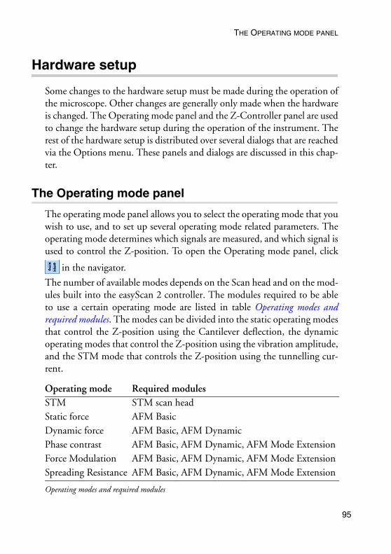
THE OPERATING MODE PANEL
Hardware setup
Some changes to the hardware setup must be made during the operation of the microscope. Other changes are generally only made when the hardware is changed. The Operating mode panel and the Z-Controller panel are used to change the hardware setup during the operation of the instrument. The rest of the hardware setup is distributed over several dialogs that are reached via the Options menu. These panels and dialogs are discussed in this chap-ter.
The Operating mode panel
The operating mode panel allows you to select the operating mode that you wish to use, and to set up several operating mode related parameters. The operating mode determines which signals are measured, and which signal is used to control the Z-position. To open the Operating mode panel, click
in the navigator.
The number of available modes depends on the Scan head and on the mod-ules built into the easyScan 2 controller. The modules required to be able to use a certain operating mode are listed in table Operating modes and required modules. The modes can be divided into the static operating modes that control the Z-position using the Cantilever deflection, the dynamic operating modes that control the Z-position using the vibration amplitude, and the STM mode that controls the Z-position using the tunnelling cur-rent.
Operating mode Required modulesSTM STM scan headStatic force AFM BasicDynamic force AFM Basic, AFM DynamicPhase contrast AFM Basic, AFM Dynamic, AFM Mode ExtensionForce Modulation AFM Basic, AFM Dynamic, AFM Mode ExtensionSpreading Resistance AFM Basic, AFM Dynamic, AFM Mode Extension
Operating modes and required modules
95

HARDWARE SETUP
96
The signals measured with each of the operating modes are listed in table Operating modes and measured signals. Note that the names of the signals can be changed in the ‘Scan Head Calibration’ dialog.
STM modeThis mode is only available when an STM head is connected to the control-ler. In this case, it is the only available mode setting.
Operating mode (Easy, Standard, Advanced)
Mounted cantilever (Easy, Standard, Advanced)Not available, this input is only used for AFM modes.
Operating mode (Easy, Standard, Advanced)STM mode by default.
Operating mode Signals measured Static force Topography, Cantilever deflection(, User Input 1,
User Input 2)Dynamic force Topography, Vibration amplitude(, User Input 1,
User Input 2)Phase contrast Topography, Vibration amplitude, Vibration
phase(, User Input 1, User Input 2)Force modulation Topography, Cantilever deflection, Vibration
amplitude(, User Input 1, User Input 2)Spreading Resistance Topography, Cantilever deflection, Tip current(,
User Input 1, User Input 2)STM Topography, Tip Current (User Input 1, User
Input 2)
Operating modes and measured signals: The User Inputs are only available when they are enabled and the Signal Module: A is installed.

THE OPERATING MODE PANEL
User Input/Output (Standard, Advanced)See the description under Static Force mode.
Static Force modeIn the static force mode, the Operating Mode and User Input sections are available.
Operating mode (Easy, Standard, Advanced)
Mounted cantilever (Easy, Standard, Advanced)The mounted cantilever type. The mounted cantilever type is used to auto-matically determine the search range in the dynamic operating modes, and to determine the correct calibration for the force set point in the static oper-ating modes.
Operating mode (Easy, Standard, Advanced)Changes the operating mode.
User Input (Standard, Advanced)Enable User Input1, 2
When active, the data from the User input (chapter The Signal Modules(p.72)) is measured and stored. Enabling the user inputs significantly increases the measurement file size.
97
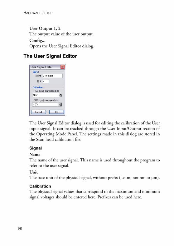
HARDWARE SETUP
98
User Output 1, 2The output value of the user output.
Config...Opens the User Signal Editor dialog.
The User Signal Editor
The User Signal Editor dialog is used for editing the calibration of the User input signal. It can be reached through the User Input/Output section of the Operating Mode Panel. The settings made in this dialog are stored in the Scan head calibration file.
SignalNameThe name of the user signal. This name is used throughout the program to refer to the user signal.
UnitThe base unit of the physical signal, without prefix (i.e. m, not nm or µm).
CalibrationThe physical signal values that correspond to the maximum and minimum signal voltages should be entered here. Prefixes can be used here.

THE OPERATING MODE PANEL
Dynamic Force modeIn addition to the same Operating mode and the User Input section as in the static operating mode, two sections of parameters may be available, depending on the user interface mode.
The dynamic force mode parameters can either be set manually or deter-mined using an automatic search procedure. The automatic search starts with the coarse measurement of a cantilever resonance curve (figure Deter-mination of the vibration frequency). Throughout this measurement, the
cantilever is excited with a fixed amplitude, whilst the excitation frequency is varied. The resonance curve contains a measurement of the resulting can-tilever vibration as a function of the excitation frequency. When the search is successful, the resonance curve contains a single peak at the free resonance frequency of the cantilever. Afterward, a second, fine-tuning search is per-formed in a 3 kHz frequency range around the resonance frequency detected in the coarse search.
The computer adjusts the value of Vibration frequency so that the canti-lever vibration amplitude is reduced by the amount set in ‘Amplitude reduc-tion’ in the Freq. Peak Search section.
Mode Properties (Easy, Standard, Advanced)Free vibration amplitude (Easy, Standard, Advanced)The desired reference amplitude of the cantilever vibration. The cantilever vibrates at this amplitude when it is far away from the sample. The excita-
Determination of the vibration frequency
frequency
vibr
atio
n am
plit
ude
free resonancefrequency
vibrationfrequency
amplitudereduction
99

HARDWARE SETUP
10
tion strength is adjusted so that this vibration amplitude is reached.
Vibration frequency (Standard, Advanced)The frequency at which the cantilever vibrates during the measurement. This frequency can automatically be set as described at the start of this sec-tion. When ‘Auto set’ is enabled, the Vibration frequency is automatically set each time an approach is started. Clicking starts the automatic setting immediately.
Display sweep chart (Standard, Advanced)When active, the results of the vibration frequency search measurements are transferred to a measurement document, and displayed on the screen.
Freq. peak search (Advanced)The parameters for the automatic vibration frequency search are set here.
Start frequency (Advanced)The start frequency for the coarse search
End frequency (Advanced)The end frequency for the coarse search
Cantilever resonance curve: left: coarse search; right: fine-tuning search
0

THE OPERATING MODE PANEL
Step frequency (Advanced)The difference between two frequency points at which the cantilever vibra-tion amplitude is measured during the coarse search. If the increment is large, the search takes less time. When however the increment is too large, there is a risk that the resonance frequency may not be found.
Auto set (Advanced)When active, the range and frequency increment are automatically set to suitable values for currently selected cantilever type.
Amplitude reduction (Advanced)Indirectly determines the ‘Vibration Frequency’ in the ‘Auto set’ mode: The computer adjusts the Vibration frequency so that the cantilever vibration amplitude is ‘Amplitude reduction’ percent smaller than the vibration amplitude at the resonance frequency.
Use upper sideband (Advanced)When active, the vibration frequency is set larger than the resonance fre-quency. Otherwise, the vibration frequency is set smaller.
Phase Contrast modeIn addition to the parameters in the Dynamic Force operating mode, the Reference Phase is available in the Standard and Advanced user interface modes.
Reference Phase (Standard, Advanced)The reference phase for the detected cantilever vibration. Changing the ref-erence phase changes the offset of the phase signal. The phase reference can
101

HARDWARE SETUP
10
be automatically set so that the phase signal is zero. When ‘Auto set’ is ena-bled the phase reference is automatically set after finishing the approach. Clicking starts the automatic setting immediately.
Force Modulation modeIn addition to the parameters in the Static Force operating mode, two addi-tional parameters are available.
Excitation amplitudeThe amplitude of the sensor excitation during a force modulation mode measurement.
Excitation frequencyThe frequency of the sensor excitation during a force modulation mode measurement. Clicking starts a measurement of the cantilever reso-nance curve, that helps you to select the excitation frequency. The settings for this measurement are the same as those for the Dynamic Force measure-ment.
Spreading Resistance modeThe operating mode panel for the Spreading Resistance mode is the same as that for Static Force operating mode.
The Z-Controller Panel
The tip-sample interaction is normally kept constant using the Z-Control-ler. The Z-Controller is a PI(D) controller as is shown in figure Z- Control-ler. The settings of this controller are set in the Z-Controller panel. To open
the Z-Controller panel, click in the Navigator.
Z-Controller (Easy, Standard, Advanced)Set point (Easy, Standard, Advanced)The working point for the Z-Controller. Depending on the operating mode, this is the tunneling current (STM mode), cantilever deflection (static force mode) or relative cantilever vibration amplitude (dynamic force mode). In the latter case, the set amplitude is relative to the operating amplitude, set in the Operating mode panel. For example, when a set point
2

THE Z-CONTROLLER PANEL
of 70% is used, the Z-Controller will move the tip closer to the sample until the vibration amplitude has decreased to 70% of the vibration amplitude far away from the sample.
Loop-Gain (Easy)The speed of the Z-Controller. If the gain is too low, the Z-Controller will not follow the surface fast enough. Thus, the image will not be as sharp as it could be. If the gain is too high, the Z-Controller will overshoot and may start to oscillate. Thus, the image will contain many measurement artifacts.
P-Gain (Standard, Advanced)The strength of the Z-Controller reaction that is proportional to the error signal. Increasing the P-Gain decreases the error signal.
I-Gain (Standard, Advanced):The strength of the Z-Controller reaction that is proportional to the inte-gral of the error signal. Increasing the I-Gain decreases the error signal over time. It is the least sensitive to noise, and usually the dominant contributor
Z- Controller
Set point
Topography
ErrorSignal+
-
+Control Signal (Tip Current,Deflection, Amplitude, ...) 1..16x
ErrorRange
P-Gain
D-Gain
I-Gain
dt
d dt
+
+
103

HARDWARE SETUP
10
to the topography measurement.
D-Gain (Advanced)The strength of the Z-Controller reaction that is proportional to the deriv-ative of the error signal. Increasing the D-Gain decreases fast changes in the error signal, but also amplifies high frequency noise. The D-Gain is only available in the ‘Standard PID’ Z-feedback mode of the Z-Controller (see following section).
Z-Controller Mode (Advanced)
Z-Feedback Mode
Free Running The Z-Controller is active.
Freeze Position The Z-Controller is not active, the scanner remains in its current Z-position.
Stop and Clear The Z-Controller is not active, the scanner is moved to the ‘Ref. Z Plane’, set in the Imaging Panel.
The Probe Status light will blink green as long as the Z-Controller is deacti-vated.
IMPORTANTThe tip may be damaged when the Z-Controller is not active during scan-ning. This will definitely happen when Ref. Z Plane is much lower than the current position of the tip, or when the scan range contains large height differences.
Z-Feedback algorithm
Standard PID A standard PID controller is used for Z-Feedback.
Adaptive PI A standard PI controller is used for feedback. In addi-
4

CANTILEVER TYPES CONFIGURATION
tion, the bandwidth of the Topography measurement is adapted to the number of measured points per sec-ond.
The adaptive PI controller reduces noise in the measurement. However, topography changes that happen faster than the time between two meas-ured points are also lost. This makes it more difficult to detect vibrations due to instability of the feedback loop. These vibrations remain visible in the Current, Amplitude or Deflection signal. Therefore, always monitor these signals when optimising Z-Controller settings, especially when using the Adaptive PI setting.
Error Range (Advanced)The range of the error signal used to control the Z-Position. The error sig-nal is the difference between the signal used for topography feedback and the current set point. When the value of ‘Error Range’ is reduced, the reso-lution of the error signal is increased.
Tip Properties (Standard, Advanced)
Tip Voltage (Standard, Advanced)The potential to be applied to the tip. The usable voltage range is between -10V and +10V. In the STM, the sample is automatically connected to the ground of the instrument. In the AFM, the sample has to be electrically connected to the instrument chassis ground for accurate measurements.
Cantilever types configuration
The cantilever types that you can select from in the Operating Mode Panel are configured using two dialogs: The cantilever browser, and the cantilever editor dialog. The cantilever types configuration is stored in a file called ‘cantilever.ini’, located in the local settings directory of the user logged on to the PC.
105

HARDWARE SETUP
10
The cantilever browser dialog
The cantilever browser dialog is opened via the menu ‘Options>Config Cantilever Types...’. The cantilever browser allows the editing and creation of cantilever types.
NewOpens the cantilever editor dialog for a new cantilever type. You can create new cantilever types that are not defined in the default configuration. The AFM head requires the following cantilever properties:
• The bottom of the sensor chip must have grooves that fit into the align-ment chip.
• The cantilever should have a nominal length of 225 µm or more, and a width of 40 µm or more.
• The back of the cantilever must have a coating that reflects infrared light. Uncoated cantilevers transmit much of the infrared light of the deflection detection system.
Edit...Opens the cantilever editor dialog to modify the currently selected canti-lever type.
Delete...Deletes the currently selected cantilever type using the cantilever editor dia-log.
6

SCAN HEAD CONFIGURATION
The cantilever editor dialog
The following properties of a cantilever type are entered in this dialog:
Name of cantileverThe name of the cantilever type. This name appears in the cantilever browser and the Cantilever type drop-down in the Operating Mode Panel.
Spring constantThe (nominal) spring constant of this cantilever type. This value is used to calculate the correct force Set point in the operating modes that use the static force for Z-Control. (section Static Force mode (p.97))
Resonance frequencyThe (nominal) resonance frequency of the cantilever type. This frequency is used for the calculation of the automatic resonance frequency search range (section Dynamic Force mode (p.99)).
Scan head configuration
The scan head configuration is used to store all calibration values specific to a certain scan head. The configuration of each scan head is stored in a file with the extension ‘.hed’. This file is copied from the software installa-tion CD on installation of the instrument. When you change the scan head, you should also load the correct configuration file.
The scan head selector dialogThe scan head selector dialog is opened via the menu ‘Options>Config Scan Head...’.
107

HARDWARE SETUP
10
Load...Loads a different scan head configuration file.
Save as...Saves the current scan head configuration under another name.
Edit...Edit the currently loaded scan head configuration using the scan head cali-bration dialog. Always save a backup of the Scan head configuration by clicking ‘Save As...’.
The scan head calibration editor
In this window the calibration of all standard Inputs and Outputs can be configured individually along with some scanner. The configuration of the User inputs and outputs is located in a different dialog (section The User Signal Editor (p.98)).
IMPORTANT Changes to these settings should be performed with great care. False set-tings can lead to false interpretation of the data and incorrect operation of the controller.
8

SCAN HEAD CONFIGURATION
Scan Axis, Maximum scan rangesX/Y/Z-Axis RangeThe calibration values of each of the scanner axes. The calibration values are given as the maximum motion range of the scanner (when Overscan is set to 0%).
SetOpens the scan axis correction dialog (see next section).
Scan Axis, Axis OrthogonalityThe X- and Y-Axes of the scanner are generally not perfectly orthogonal, and their orientation with respect to the AFM housing may vary. The easy-Scan software corrects these errors by adding/subtracting some of the X scanner command signal to the Y scanner command signal and vice versa.
X/Y AngleThe angle between then the X and Y axis of the scanner hardware. The software uses this value to correct the scan command signals such that the scan axes are orthogonal.
RotationThe angle between the X axis of the scanner and the X axis of the micro-scope body (figure Scanner coordinate system (p.86)). The software uses this value to correct the scan command signals such that the scan axis is parallel to the X axis of the microscope body.
I/O Signals, Maximum input signal valuesDeflectionThe calibration of the cantilever deflection signal.
AmplitudeThe calibration value of the cantilever vibration amplitude signal.
PhaseThe calibration value of the cantilever vibration phase shift signal.
Tip currentThe calibration value of the internal Tip current measurement
109

HARDWARE SETUP
11
I/O Signals, Maximum output signal valuesTip PotentialThe calibration value of the Tip voltage setting.
Drive AmplitudeThe calibration value of the Amplitude of the signal that is used to excite the cantilever. The Drive Amplitude signal is only displayed in the Data Info Panel.
The Scan Axis Correction Dialog
This dialog can be used to multiply the scan axis calibration factor by a correction coefficient that has been determined by evaluating the measure-ment of a calibration gird, for example using SPIP/Nanosurf Analysis.
Scan axis correctionThe Scan range is multiplied with this number when the ‘Set’-Button is clicked.
The Controller Configuration dialog
The Controller configuration dialog is opened via the menu ‘Options>Config Controller...’. On a correctly configured system, it should not be necessary to change the settings in this dialog, except for the start-up parameters and chart arrangement file configuration.
0
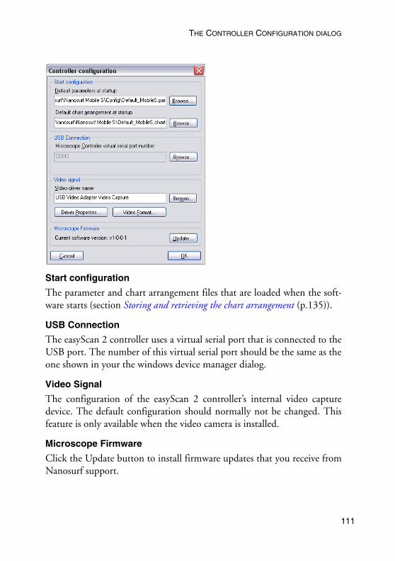
THE CONTROLLER CONFIGURATION DIALOG
Start configurationThe parameter and chart arrangement files that are loaded when the soft-ware starts (section Storing and retrieving the chart arrangement (p.135)).
USB ConnectionThe easyScan 2 controller uses a virtual serial port that is connected to the USB port. The number of this virtual serial port should be the same as the one shown in your the windows device manager dialog.
Video SignalThe configuration of the easyScan 2 controller’s internal video capture device. The default configuration should normally not be changed. This feature is only available when the video camera is installed.
Microscope FirmwareClick the Update button to install firmware updates that you receive from Nanosurf support.
111

HARDWARE SETUP
11
The Edit Access Codes Dialog
The Edit Access Codes Dialog is used to enter the access code for software modules. At the moment, the only software module is the scripting inter-face. The dialog is accessed via the menu entry ‘Options>Config Access Codes...’
The Scan head Diagnosis dialog
The Scan head Diagnosis dialog is opened via the menu ‘Options>Check Scan Head...’. In it, the controller reports the current status information of the sensor or the approach platform. If the Status light on the easyScan 2 controller is blinking red, more detailed information about the failure is displayed in the ‘Microscope Diagnosis’ dialog.
Simulate Microscope
Check or uncheck the menu item ‘Options>Simulate Microscope’ to enter and exit the simulation mode. Once the simulation mode is active, the first field in the status bar of the easyScan 2 software displays the text ‘Simula-tion’, otherwise this field displays the text ‘Online’.
2

THE ABOUT DIALOG
In the simulation, many functions of the microscope are performed on a mathematically generated surface. Thus, the software functionality and working methods of the microscope can be practised.
The About dialog
The About dialog displays various information that may be useful for diag-nostics when you have problems with your instrument. To open the About dialog:
- Select the menu entry ‘?>About...’.
The about dialog contains the following information:
• the version number of the control software
• the serial number of the controller
• the version number of the firmware that is running on the controller
• the version number of the built-in modules
113

HARDWARE SETUP
11
• contact information for getting more support.
When the microscope simulation is active, the about dialog displays the serial number ‘000-00-000’ is displayed. The Nanosurf Web site and con-tact address for information and software updates are also displayed here.
4

THE APPROACH PANEL
Positioning
The Positioning window contains all the software tools for positioning the tip with respect to the sample:
• The Approach panel
• The Video panel (with the Video Module)
• The Video display (with the Video Module)
Click in the Navigator to open the Positioning window.
The Approach panel
The motor for the tip-sample approach is operated using the ‘Approach Panel’.
115

POSITIONING
11
Approach (Easy, Standard, Advanced)
StatusDisplays the current status of the approach stage.
Increases the tip-sample distance at maximum speed until the button is released.
Decreases the tip-sample distance at maximum speed until the button is released.
Increases the tip-sample distance with the settings given in the Approach Options.
Starts the automatic approach. During the automatic approach, the tip-sample distance is decreased until the Set point, set in the Z-Controller panel, is reached, or until the maximum approach time is reached.
6

THE APPROACH PANEL
Approach Options (Standard, Advanced)
Tip-Position (Advanced)Determines the Z-Position of the scanner when the approach motor stops. When the Tip-Position is changed when the tip is already approached to the sample, the motor will move the approach stage so, that the Z-Position of the tip becomes equal to the set Z-Position. When a high resolution (2 µm Z-Range) scanner is used, the Tip-Position before the approach is set to +500 nm Advanced by default. This compensates for the residual motion of the approach stage that occurs after the approach motor has stopped.
CAUTIONChanging the Z-Position when the tip is approached to the sample may cause tip damage when using high resolution scanners. This can be due to play in the approach stage, which is caused by a change in the initial load of the approach stage bearings. Contact your local Nanosurf representative if this seems to be the case.
The Tip-Position setting can for example be useful when a sample is mainly a large flat surface with some deep holes in it. In this case proceed as follows:
- Ideally, first make sure that the center position of the Scan range is outside a hole.
When the Scanner is idle (such as during approach), the tip is always brought to the center position of the scan range.
- Set Tip-Position to about 80% of the maximum value.
117

POSITIONING
11
- Click Approach
The Tip-Position setting can not be used with STM scan heads, which is due to the different approach motor used in the STM.
Stop buttonStop the adjustment of the height
Appr. speed (Standard, Advanced)The speed of the motor during the automatic approach and withdraw. When an STM scan head is used, the Approach speed changes the Step size of the approach motor, the step frequency is determined by the speed of the feedback loop.
CAUTIONIf the approach is too fast, the tip or the sample surface can be damaged. On the other hand, the motor will not move when Appr. speed is too small.
Max. Withdraw (Standard, Advanced)The maximum withdraw duration after clicking .
Max. Approach (Advanced)The maximum approach duration after clicking .
Auto. start imaging (Standard, Advanced)When selected, the system automatically starts imaging after a successful approach. Scanning is automatically stopped when the approach motor is moved.
Auto reload settings (Advanced)When selected, the software reloads the default start-up parameter file each time an approach is started (section The Controller Configuration dialog(p.110)).
The Video panel
The video panel controls the video display in the Positioning window.Changing these settings only has effect when a Video camera is fitted on your system.
8

THE VIDEO PANEL
Video source
The video source section determines which video signal is currently dis-played.
Switches the video display to the top view.
Switches the video to the side view.
Saves the currently displayed image to a JPEG file that is selected using a Save file as... dialog.
Video Options
The Video Options section determines how the video signal is displayed. There are separate sets of options for the side and the top view.
IlluminationThe intensity of the sample illumination on the scan head.
BrightnessThe brightness of the video display
ContrastThe contrast of the video display
119

IMAGING
12
Imaging
Imaging measurements of the sample are controlled using the Imaging win-
dow. The Imaging window can be opened by clicking in the navigator. The Imaging window contains the Imaging bar, with commands that con-trol the imaging processes, and the Imaging panel, with parameters that determine how the imaging is done.
The Imaging window also contains a number of charts that display the data from the ongoing measurement. The imaging window can display as many charts as the size of the window can accommodate. By default, two charts are displayed, a Line graph, and a Color map of the sample’s Topography. For more information on adding and changing charts (chapter Viewing measurement data (p.134)).
The imaging window
0

THE IMAGING BAR
The imaging bar
/ starts a measurement and then changes to . Clicking
aborts the measurement as soon as the current scan line is finished.
After clicking the measurement stops when the current measurement has finished.
/Starts a single measurement or changes the scanning direction of the meas-urement in progress. With the image is scanned from the bottom to top, with it is scanned from the top to the bottom. If a measurement has been started using or the measurement stops automatically after one full image.
Selects an area that is to be measured in more detail. The size and area of the area is displayed in the Tool Results panel.
One corner of the zoomed area is defined by the mouse cursor position where the left mouse button is clicked, the opposite corner by the position where the button is released. When the mouse is not moved between click-ing and releasing, an area is defined that has a size of 33% of the current measurement, and centred on the clicked location. Once an area is defined,
121

IMAGING
12
it can be resized by dragging one of its corners, and moved to the desired position by dragging its centre point.
A double click with the left mouse button in the chart, or clicking the Zoom button in the Tool Results panel, modifies the parameters Scan range, X-, Y-Offset in the Imaging window accordingly. When the zoom function is active it can be aborted by clicking again.
Moves the position of the imaged area. An interesting corner can thus be moved to the centre of the measurement. The Tool Results panel numeri-cally displays the change in position.
The change in the position is indicated by an arrow. The start of the arrow is defined by the mouse cursor position where the left mouse button is clicked, the end of the arrow by the position where the button is released. When the mouse is not moved between clicking and releasing, an arrow ending in the centre of the measurement is drawn. The direction of the arrow can be adjusted by dragging its end markers, it can be moved by dragging the centre marker.The image is moved by double clicking, or clicking the Move button in the Tool Results panel. The move function can be aborted by clicking again.
Returns the parameters Scan range to the largest possible values, and ‘X-
2

THE IMAGING PANEL
Offset’ and ‘Y-Offset’ to zero.
Transfers the current measurement data to the spectroscopy window. If a measurement is in progress, it is interrupted. It is advisable to use to complete the current measurement before starting the spectroscopy meas-urement.
Captures the measurement currently displayed in the ‘Imaging window’ in a measurement document.
If is clicked when a scan is in progress, a new measurement document is generated each time a measurement is finished. The capture process is cancelled by clicking a second time.
To capture an image without waiting for the scan to be completed, stop the scanning by clicking . The image can then be captured immediately by clicking .
The measurement documents are labelled automatically with increasing numbers (i.e. Image1, Image2,...). When leaving the program you will be asked if you want to save the unsaved measurement documents.
The Imaging panel
The imaging settings use two coordinate systems: The Scanner coordinate system and the Measurement image coordinate system. To separate the two systems, the image axes are denoted by an asterisk (i.e. X*, Y*). The relation between the two coordinate systems is determined by various parameters in the imaging panel. The effect of these parameters is illustrated in figure Coordinate systems.
Imaging Area (Easy, Standard, Advanced)Image size (Easy, Standard)The image size in both the X* and Y* direction. The size is doubled or halved when using .
Image width (Advanced)The image size in X* direction.
123

IMAGING
12
Height (Advanced)The image size in Y* direction. When the Check-box is active, the image Height is always identical to the Image width.
Points / Line (Easy, Standard, Advanced)The number of measured data points per line.
Lines (Advanced)The number of measured data lines in an image. When the Check-box is active, the number of Lines is always equal to the number of Points / Line. In the easy and standard user interface mode, the number of Lines is always equal to the number of Points / Line.
Time / Line (Easy, Standard, Advanced)The time needed to acquire a data line. The time needed for the entire image is approximately:
Coordinate systems
XY
Z, Z*
Scanner XY-plane
'X-Slope' angle
'Y-Slope' angle
'Rotation' angle
Measurement plane
Image areaX*Y*
Image time ´Time / Line´ ´Lines / Frame´ 2⋅ ⋅=
4

THE IMAGING PANEL
Rotation (Easy, Standard, Advanced)The angle between the X-direction of the scanner and the X* direction of the measurement (figure Coordinate systems).
Imaging Options (Standard, Advanced)
The reference plane for the image can be aligned to the surface of the sam-ple using the slope parameters (figure Coordinate systems).
X-Slope (Standard, Advanced)A positive value rotates the image plane around the Y-axis in the counter-clockwise direction.
Y-Slope (Standard, Advanced)A positive value rotates the image plane around the X-axis in the counter-clockwise direction.
The centre position of the measured area can be changed by typing its posi-tion as well as by using the Move tool in the imaging bar. The zero position is the centre position of the scanner.
Image X-Pos, Y-Pos (Advanced)The centre position of the measured area.
Overscan (Standard, Advanced)The amount by which the scan range of each line is made larger than the measurement range, relative to the image width. Thus edge effects, caused by the reversal of the scanning motion, are not displayed in the measure-ment. Disadvantages of using Overscan are that the maximum scan range is reduced, the tip moves slightly faster over the sample with the same ‘Time/Line’ setting, and the tip may hit large features outside the measured image. The value of ‘Overscan’ determines how much the scan range is
125

IMAGING
12
increased relative to the Image width.
Ref. Z-Plane (Advanced)The height of the reference plane. This height reference is used when the Z-Controller output is cleared, and when the Z-position is not modulated relative to the current surface position during spectroscopy measurements.
Imaging Modes (Advanced)
Scan modeThe Y* direction in which the data is acquired and displayed:
Continuous the acquisition direction is reversed after each scan: from bottom to top and vice versa
Cont.Up from bottom to top
Cont.Down from top to bottom
Measurement modeThe X* direction in which the data is acquired and stored:
Forward during forward scan only (left to right in the image)
Backward during backward scan only (right to left in the image)
Forw.&Backw. during both forward and backward scan
Const.-Height modeWhen the Constant Height Imaging mode is enabled, the Z-Controller is turned off during the scan (as a consequence, the Sensor Status light will blink green). Instead, the scanner scans along a straight line, that should be parallel to the surface. The slope of the line is defined by the X- and Y-Slope parameters in the Imaging Options section of the Imaging Panel. These parameters should be set as described in section Adjusting the measurement
6

THE IMAGING PANEL
plane (p.54). The height of the line is determined at the start of each scan line: First the Z-Controller is turned on. Once the tip position is stable, the Z-Controller is turned off and the tip is moved away from the sample by the distance set by the parameter Rel. Tip-Pos.
The Constant Height Imaging mode is mainly useful for EFM and MFM measurements. For more information on how to do Magnetic Force Microscopy, refer to technical note TN00031 Magnetic Force Microscopy, which can be downloaded from the support section of the Nanosurf web site at www.nanosurf.com.
Rel. Tip-PosThe distance by which the Tip is moved towards the sample from the posi-tion that corresponds to the set point. A negative setting will move the tip away from the sample.
127

SPECTROSCOPY
12
Spectroscopy
In a spectroscopic measurement, the input channels are measured as a func-tion of a modulated parameter. This modulated parameter can be the Z-distance to the sample, the tip voltage, or a User output channel (when the Signal Module: A is installed). Note that you must electrically connect the sample to the ground connector on the easyScan 2 AFM AFM scan head to apply a tip-sample voltage difference. The measured parameter can be any available input channel. Examples of a spectroscopic measurements are force/distance curves in the AFM static force mode, amplitude/voltage curves in the AFM dynamic mode, or current/voltage curves with the STM.
The accuracy of the spectroscopic measurements can be increased by aver-aging the measurement results of several consecutive modulations. A spec-troscopic measurement sequence consists of a number of spectroscopic measurements of the same type, measured along a user defined line in the XY-plane. A point measurement is made if the number of points is one. The measurement sequence is carried out as follows:
1. The tip is moved with active Z-control to the start of the line.
2. The Z-Controller is switched off.
Spectroscopy window
8

THE SPECTROSCOPY BAR
3. A spectroscopic measurement is recorded.
4. The Z-Controller is turned on again.
5. The tip is moved to the next point on the line in the XY-plane.
Steps 2.-5. are repeated for each points on the line.
Spectroscopic measurement sequences are controlled using the Spectros-copy window. The Spectroscopy window can either be opened by clicking
in the navigator, or by clicking in the Imaging bar. When the Spectroscopy window is activated from the Imaging bar, the currently measured image is transferred to the Spectroscopy window.
The Spectroscopy window contains the Spectroscopy bar, with commands that control the spectroscopy processes, and the Spectroscopy panel, with parameters that determine how the spectroscopy measurement is done.
The Spectroscopy window also contains a number of charts that display the data from a previous imaging measurement and the data from the ongoing spectroscopic measurement. The Spectroscopy window can display as many charts as the size of the window can accommodate. It is recommended to display at least two charts, one a Color map of a previous Topography meas-urement of the area where the spectroscopy measurement is performed, and one a Dual Line graph of the current spectroscopy measurement. For more information on adding and changing charts (chapter Viewing measurement data (p.134)).
The Spectroscopy bar
/ starts a spectroscopy measurement sequence and then changes to until the measurement sequence is finished. Clicking aborts the
measurement sequence as soon as the current modulation period is fin-ished.
/Starts the selection of the XY measurement position(s) in a topography Color map chart using the mouse cursor. These positions are automatically transferred to the appropriate entries in the Position section of the Spectros-
129

SPECTROSCOPY
13
copy panel. When selecting a line, clicking the chart once creates a line from the clicked position to the centre of the image.
Captures the measurement currently displayed in the Spectroscopy window in a measurement document, and displays it in a separate window.If is clicked during the measurement, a copy is generated when the measurement in progress is finished. During the measurement, the button remains pressed. The capture process is cancelled by clicking a second time.
The measurement documents are labelled automatically with increasing numbers (i.e. Image1, Image2,...). When leaving the program you will be asked if you want to save the unsaved measurement documents.
The Spectroscopy panel
Modulation (Easy, Standard, Advanced)
Modulated output (Easy, Standard, Advanced)The number of available modulated outputs depends on the scan head and the number of installed modules operating modes that are available. Possi-ble values are: ‘Z-Axis’, ‘Tip Potential’ and the names of the User Outputs.
Start value/End value (Easy, Standard, Advanced)The range over which the Modulated output is changed. The ‘Spec For-ward’ data is measured from the Start to the End value, the ‘Spec backward’ data is measured in the opposite direction. The ‘Spec forward’ data is always measured before the ‘Spec backward’ data.
0

THE SPECTROSCOPY PANEL
Relative to current value (Standard, Advanced)When active, the Start and the End values are added to the value the mod-ulated output had before starting the modulation.When the Tip Potential is modulated, the current value is the Tip voltage set in the Z-Controller panel. When the Z-Axis is modulated, the current value is the sample surface height, as measured using the Z-Controller output. Otherwise, the meas-urement z-position is given by the value of the Ref. Z-Plane in the Imaging Panel.
Modulation time (Easy, Standard, Advanced)The time used to change the Modulated output from the Start to the End value.
Keep Z-Controller active (Advanced)The Z-Controller will continue to change the Z-position so as to keep tip-sample interaction constant. This option is not available when the Modu-lated output is set to the Z-Axis. This setting can for example be used to measure tip current as a function of applied voltage whilst keeping the tip-sample force constant.
Measurement (Easy, Standard, Advanced)
Data points (Easy, Standard, Advanced)The number of data points in one spectroscopic measurement. The data points are equally distributed over the modulation range.
Averages (Easy, Standard, Advanced)The number of times the modulation is repeated to obtain an averaged spectroscopic measurement. The measurement results of aborted modula-
131

SPECTROSCOPY
13
tions are discarded during averaging.
Input range check (Standard, Advanced)In order to prevent tip damage due to too high tip-sample interaction, the settings below ‘Input range check’ define a safe range of tip-sample interea-cion. When the interaction signal (Deflection in static modes, Amplitude in dynamic modes, Current in STM mode) leaves this safe range, the meas-urement is aborted. When a spectroscopy measurement has been aborted, a warning dialog is displayed. The number of aborts that occurred in a measurement is reported in Data Info panel as: ModAborted=<number of aborts>.
Abort action (Standard, Advanced)What is to be done when the measurement is aborted:
No range check will never abort the measurement. The tip is not pro-tected against damage due to too high tip-sample interaction. This is the default setting.
Abort modulation aborts the current modulation period, and continues with the next modulation until the number of modu-lations in ‘Averages’ is reached.
Abort current measurementaborts the spectroscopy measurement for the current point and continues with the next point of the line, if a spectroscopy is being performed.
Abort measurement sequenceaborts the entire spectroscopy measurement sequence (cancels all ‘Averages’ and points).
Max / Min input value (Standard, Advanced)The Minimum/maximum value that the feedback signal is allowed to have.
Position (Easy, Standard, Advanced)The Position parameters can be used to define a sequence of spectroscopy measurements on positions that are equally distributed over a line.
Sequence Points (Easy, Standard, Advanced)The number of Spectroscopy Measurements to be made in the sequence.
X-Pos from/Y-Pos from (Easy, Standard, Advanced)The XY-coordinates of the measured point in a -spectroscopy measure-
2

THE SPECTROSCOPY PANEL
ment. Sets the XY-coordinates of the starting point of the line in a -spectroscopy measurement sequence.
X-Pos to Y-Pos to (Easy, Standard, Advanced)The XY-coordinates of the end-point of the line in a -spectroscopy measurement sequence.
The from and to coordinates are more conveniently chosen using the or tools in the Spectroscopy bar.
133

VIEWING MEASUREMENT DATA
13
Viewing measurement data
Measurement data are displayed in charts. Charts are used in Measurement document windows, the Imaging window and the Spectroscopy window. The measurement settings are displayed in the Data Info panel.
Charts
A Chart is a graphical representation of the measured data, and additional elements that give information about the chart itself (figure Elements of a Chart).
These elements show the displayed Signal, Chart type, the type of Filtering applied to the data, and the Color scale used to display the data. The Color scale shows which measured signal level is mapped to which colour. The colour mapping can be changed using the Color Palette dialog, described further on in this section. The Data range indicator shows the range of possible measurement values that is occupied by the measured data.
The Chart bar is used to create new charts and to modify their properties. The chart configuration of the Imaging and Spectroscopy window can be saved to a file. The chart configuration of the measurement documents is saved together with the document.
Elements of a Chart
Signal
Line selection arrow
Data range indicator
Color scale
Data filter
Chart range
4

THE CHART BAR
Storing and retrieving the chart arrangementThe chart arrangement of the Imaging and Spectroscopy windows is stored in a configuration file with the extension ‘.chart’. When the easyScan 2software is started, a default arrangement is loaded from a file that is selected in the Controller Configuration dialog (section The Controller Configuration dialog (p.110)). Functions for storing and retrieving the chart arrangement are accessed via the menu ‘File>Chart Arrangement’.
‘Save’ saves the chart arrangement to the currently selected chart file. The name of this file is indicated in the status bar at the bottom of the main window.
‘Save as...’, saves the chart arrangement under a new file name.
‘Load’ loads a previously saved chart file.
IMPORTANTWhen you have not loaded another file, ‘Save’, will overwrite the original default chart arrangement file with the current settings.
The Chart bar
The properties of the charts are set using the Chart bar. The settings dis-played in the Chart bar refer to the currently active chart. This chart is indicated by a grey line around the chart. A Chart is activated by clicking it with the mouse cursor.
The following buttons control the creation and modification of the charts.
(Create new Chart)Creates a copy of the currently active chart and adds it as the last chart in the active window. Charts are first ordered top to bottom, then left to right. The window may have to be resized to see all charts.
(Delete Current Chart)Removes the currently active chart.
(Chart type)The chart type:
Line graph data is displayed as a plot. Points outside the range of
135
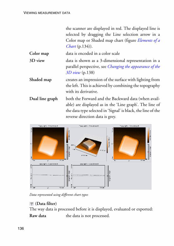
VIEWING MEASUREMENT DATA
13
the scanner are displayed in red. The displayed line is selected by dragging the Line selection arrow in a Color map or Shaded map chart (figure Elements of a Chart (p.134)).
Color map data is encoded in a color scale
3D view data is shown as a 3-dimensional representation in a parallel perspective, see Changing the appearance of the 3D view (p.138)
Shaded map creates an impression of the surface with lighting from the left. This is achieved by combining the topography with its derivative.
Dual line graph both the Forward and the Backward data (when avail-able) are displayed as in the ‘Line graph’. The line of the data type selected in ‘Signal’ is black, the line of the reverse direction data is grey.
(Data filter)The way data is processed before it is displayed, evaluated or exported:
Raw data the data is not processed.
Data represented using different chart types
6
THE CHART BAR
Mean fit the mean value of each line of data points is calculated and then subtracted.
Line fit the best fit line for each line of data points is calculated and then subtracted.
Derived data the difference between two successive data points (derivative) is calculated.
Parabola fit the best fit parabola for each line of data points is cal-culated and then subtracted.
Polynomial fit the best fit fourth order polynomial for each line of data points is calculated and then subtracted.
(Signal)The input channel that is displayed. The available signals depend on the operating mode, the status of the User input (section The Operating mode panel (p.95)) and the measurement mode (section The Imaging panel(p.123)).
(Optimise Chart range)Adjust the chart scale so that it optimally fits the measurement data.
(Decrease Chart range)Halves the chart scale, thereby increasing feature contrast / height.
(Increase Chart range)Doubles the chart scale, thereby decreasing feature contrast / height.
(Chart properties dialog)Opens the chart properties dialog.
The Chart properties dialog
Chart rangeSpanThe signal span that corresponds to the full chart scale. Increasing Span decreases the feature contrast. The current Span is also displayed next to the color bar / axis in the chart
CenterThe signal that corresponds to the center of the chart scale.
137

VIEWING MEASUREMENT DATA
13
Auto setWhen active, the chart scale is automatically set to optimally fit the meas-urement data, as it is being acquired. Clicking has the same effect as clicking the Optimise Chart range button.
Chart sizeSizeThe size of the chart in pixels.
Show AxisWhen active, the labels in charts and the color-bar in ‘Color map’ window, are displayed.
Changing the appearance of the 3D viewAlways click and hold the left mouse button on the 3D view chart while changing the 3D view. The surface is reduced in feature complexity as long as the left mouse button is pressed. Press the following additional keys/buttons to determine what chart property is changed:
Surface rotation mouse left/right
Surface tilt mouse up/down.
Size displayed surface‘Ctrl’- key + mouse up/down
Surface position ‘Shift’-key + mouse up/down/left/right
Z-scale magnificationleft mouse button + right mouse button + mouse up/down
Light source direction (360°)‘Shift’+‘Ctrl’-key + mouse left/right
8

THE CHART BAR
Light source height (0°-90°)‘Shift’+‘Ctrl’-key + mouse up/down
The lowest height of 0° corresponds to ‘sunset’ lighting, the highest height corresponds to mid-day lighting at the equator.
The Chart Properties “Span” and “Center” can be used to cut off high and or low features of the surface.
TipTo create good-looking 3D images you can use any of the following fea-tures:
• Use the Tools ‘Correct Scan Line Level’, ‘Glitch’ and ‘Noise reduction’ filters to remove unwanted measurement artefacts.
• Set the light source direction to 90° (parallel to the scan lines)
• Click once or twice until no clipping of high features is visible (or adjust the “Span” and “Center” Properties).
The Color Palette dialog
The color palette dialog is reached via the menu item ‘Options>Config Color palette...’. The color palette is used to map the display range of the measured values to a color. Three different palette types are available:
Black&White The color map is a linear grey scale
Color The color selection uses the HSB-color model where the color (H) is set in ° value. The color is selected by
139

VIEWING MEASUREMENT DATA
14
entering a number or by clicking a color in the color bar.
Look Up Table A user definable palette (with max. 256 color entries) can be selected. This palette is stored in a ‘.lut’ file that contains an ASCII table with RGB color values. A dif-ferent look up table can be selected by clicking the ‘Browse...’ button.
The Data Info panel
The Data Info panel displays the parameters of the active measurement and the current tool results.
Data Info Panel: Display of measurement parameters
0

THE TOOL RESULTS PANEL
Quick Evaluation Tools
The easyScan 2 software has several tools that allow quick evaluation of a measurement while it is being acquired. This helps find optimal measure-ment settings. For more elaborate evaluations, the optional Nanosurf Anal-ysis or the Nanosurf Report software package can be used (section Creating a report (p.153)).
The quick evaluation tools are activated using the Tools bar or the Tools menu. The number of tools available depends on the type of the currently active chart. The evaluation results are displayed in the Tool Results panel.
IMPORTANTAll results are calculated after the ‘Data filter’ has been applied to the data. The results will generally vary when a different ‘Data filter’ option is used.
The Tool Results panel
The Tool Results panel displays the results of the currently active tool. The panel should automatically become visible when a tool is selected. To make
the panel visible, click in the navigator. The contents of the tool results panel depend on the tool that is active. It will always contain a Cursor posi-tion and a Tool status section, and may also contain a Tool result and a Tool chart section. Because the content of the Tool Results panel depends so strongly on the active tool, this panel is described in more detail with each of the tools.
The Tools bar
Properties of the measurements can be evaluated numerically using the tools. The tools are activated via the corresponding menu item or by click-ing the respective button in the tool bar. Tools can be used in all charts, both during measurement and off-line. Before using a tool on a chart, acti-vate the chart by clicking onto it. To stop using a tool, select another tool, or click its button a second time.
141

QUICK EVALUATION TOOLS
14
Measure LengthStarts measuring the distance and signal difference between two points. The measurement results are displayed in the Tool Results panel.
The two points are defined by drawing a double arrow. The first point is defined by the mouse cursor position where the left mouse button is clicked, the second point by the position where the button is released. When the mouse is not moved between clicking and releasing, an arrow parallel to the X*-axis is drawn.
The direction of the arrow can be adjusted by dragging its end markers; it can be moved by dragging the centre marker.
Measure DistanceStarts measuring the distance between two parallel lines. The measurement result is displayed in the Tool Results panel.Distance is measured by drawing two lines in the chart. The first point of the first line is defined by the mouse cursor position where the left mouse button is clicked, the second point by the position where the button is released. When the mouse is not moved between clicking and releasing, a line parallel to the X*-axis is drawn. After releasing the mouse button, a second parallel line sticks to the mouse cursor, that is released by clicking its desired position. The direction of the parallel lines can be adjusted by dragging their end markers; they can be moved by dragging the centre marker.
2

THE TOOLS BAR
Measure AngleStarts measuring the angle between features in the measurement. The meas-urement result is displayed in the Tool Results panel. In Line graph-type displays, this tool can only be used when the signal displays height data.
The angle is measured by drawing two meeting lines in the chart. The first point of the first line is defined by the mouse cursor position where the left mouse button is clicked, the second point by the position where the button is released. When the mouse is not moved between clicking and releasing, a line parallel to the X*-axis is drawn. After releasing the mouse button, the end of the second line sticks to the mouse pointer. The end is released by clicking its desired position. The angle can be changed by dragging the
143

QUICK EVALUATION TOOLS
14
line’s end point markers or the corner mark; it can be moved by dragging the line’s centre markers.
Create Cross SectionDisplays and can create a new measurement document containing a line cross-section of a Color map or Line View display. The line is displayed in the Tool Results panel. The line can be stored in a new measurement doc-ument.
The line is defined by drawing an arrow. The arrow points toward the for-ward direction of the line. The start of the arrow is defined by the mouse cursor position where the left mouse button is clicked, the end of the arrow by the position where the button is released. When the mouse is not moved between clicking and releasing, an arrow ending in the centre of the meas-urement is drawn. The direction of the arrow can be adjusted by dragging its end markers; it can be moved by dragging the centre marker.
A new measurement document containing the line section is created by double clicking the graph, or by clicking ‘Cut out line’ in the Tool Results panel.
4

THE TOOLS BAR
Cut Out AreaCreates a new measurement document containing a subsection of an exist-ing measurement. The size and area of the area is displayed in the Tool Results panel.
One corner of the area is defined by the mouse cursor position where the left mouse button is clicked, the opposite corner by the position where the button is released. When the mouse is not moved between clicking and releasing, an area is defined that has a size of 33% of the current measure-ment, and is centred on the clicked location. Once an area is defined, it can be resized by dragging one of its corners, and moved to the desired position by dragging its centre point. It is possible to define a rectangular (i.e. non-square) area by pressing the ‘Shift’ key whilst dragging a corner.
A new measurement document containing the area is created by double clicking the graph, or by clicking the ‘Cut out area’ button in the Tool Results panel.
Calculate Line RoughnessCalculates certain roughness parameters along a line. Both the selected line and calculated values are displayed in the Tool Results panel.The cross-section is selected in the same way as with the Cut out Line tool.The calculated parameters are stored in the measurement document when the ‘Store’ button in the Tool Results panel is clicked.
145

QUICK EVALUATION TOOLS
14
Calculate Area RoughnessCalculates certain roughness parameters of an area. The calculated values are displayed in the Tool Results panel.The parameters are calculated as follows:
The Roughness Average, Sa
The Valley depth, Sv
Sv = lowest value
|),(|1
0 0Σ Σ
= =
M-1
k
N-1
llk yxz
MNSa =
The Mean Value, Sm
The Peak Height, SpSp = highest value
0 0
Σ Σ= =
M-1
k
N-1
l
),(1
lk yxz MN
Sm =
The Root Mean Square, Sq
The Peak-Valley Height, SySy = Sp- Sv
0 0Σ Σ
= =
M-1
k
N-1
l
2)),((1
lk yxzMN
Sq =
6

THE TOOLS BAR
The area is selected in the same way as with the Cut out Area tool.The calculated parameters are stored in the measurement document when the ‘Store’ button in the Tool Results panel is clicked.
TipThe Area Roughness tool can be used to determine the mean height differ-ence between two plateaus with more accuracy than with the ‘Measure Dis-tance’ tool. To determine the mean height difference, select an area on each plateau, and calculate the difference between their Sm-values.
Correct BackgroundRemoves the effect of a wrong scan plane when the ‘average’ and ‘plane’ Data filter options do not give satisfactory results. This may occur when the scan lines in different parts of the measurement have a different average height. An example of such a measurement is shown in figure Correct Back-ground.To use the tool, select three points that should be on the same height. This
147

QUICK EVALUATION TOOLS
14
is done with in the same way as the angle tool. The selected points are the end points of the two connected lines.After clicking the ‘Execute’ button in the Tool Results Panel, the plane that is defined by the three points is subtracted from the measurement. To get useful results, the Data filter option for the display in which you draw the line should generally be ‘Raw data’.
Correct scan line levelsRemoves the effect of drift when the ‘average’ and ‘plane’ Data filter options do not give satisfactory results. This may occur when the scan lines in dif-ferent parts of the measurement have a different average height. An example of such a measurement is shown in figure Correct scan line levels.To use the tool, draw a line through points that should have the same height in the same way as with the Measure Length tool.After clicking the ‘Execute’ button in the Tool Results Panel, the average level of each scan line is adjusted so that all points along the drawn line have the same height. To get useful results, the Data filter option for the display in which you draw the line should generally be ‘Raw data’ or ‘Mean fit’.
Glitch FilterThe Glitch Filter removes the effect of small defects in the image such as single short glitches in the scan. Compared to the Noise Filter, it has the advantage of not reducing resolution on step edges. The glitch filter is
Correct Background: left: uncorrected image, the end points of the lines have been moved to points that should have the same height; right: corrected image
8

THE TOOLS BAR
implemented as a Median filter on a 3x3 pixel matrix.To apply the filter, activate the color map chart that is to be filtered, then click the Glitch Filter button in the Tools bar. A new Measurement docu-ment with the filtered data is created.
Noise FilterThe Noise filter removes high frequency noise from the image, but applying the filter will also decrease the resolution of the image. The Noise Filter is
Correct scan line levels: left: uncorrected image with a line through points that should be at the same height; right: corrected image
Glitch Filter: left: unfiltered image with some glitches where the tip lost contact with the sample; right: corrected image
149

QUICK EVALUATION TOOLS
15
implemented as a convolution with a 3x3 pixel Gaussian kernel function.To apply the filter, activate the color map chart that is to be filtered, then click the Noise Filter button in the Tools bar. A new measurement docu-ment with the filtered data is created.
TipFilters are especially useful for improving the appearance of 3D views.
Applying filters may changes the result of the other tools. This may result in incorrect results when evaluating sample roughness.
Noise Filter: left: unfiltered image of AFM measurement on HOPG; right: filtered image
0

STORING AND PRINTING MEASUREMENTS
Storing measurements and further data processing
Storing and Printing measurements
Storing and Printing of measurement documents can be performed using the File menu. The functions Open, Save and Print are also available via the File bar.
Menu item ‘File’ contains the items for opening , closing, saving , and printing the measurement documents and for exiting the program. In the following only the special functions are mentioned.
OpenOpens a dialog for opening Nanosurf ‘.nid’ or ‘.ezd’ (easyScan 1) files. The same dialog is opened using the menu ‘File>Open...’. It is possible to select more than one file at the same time by using the ‘Shift’ and ‘Ctrl’ keys.
‘Save’ and ‘Save as...’Save a measurement document in Nanosurf image data format (file exten-sion ‘.nid’). The same dialog is opened using the menu ‘File>Save’ and ‘File>Save as...’.
Export >Current Chart as / Current document asExports either the active chart or the whole active measurement document for use in other programs or image processing software. Available data types for documents are windows bitmap (.bmp), 16 bit data file (.dat), plot file (.plt). For Charts, additional available data types are comma separated z values (.csv), and (X,Y,Z)-points (.csv).
When the data is exported using the function ‘Export>Current document as...’, every Chart in the measurement document is stored in the export file consecutively. In the binary format, the blocks of data from each Chart are stored directly one behind the other. In the ‘ASCII’ text format the blocks of data for each Chart are separated by two empty lines.
151

STORING MEASUREMENTS AND FURTHER DATA PROCESSING
15
Windows Bitmap (.bmp)
A Windows Bitmap image is suitable for including in documents, e.g. word or image processing software. The exact image as seen on the computer screen will be saved in the file (‘screen shot’).
Data file 16Bit (.dat)
A binary data file can be processed in image processing software. This ‘binary’ data format contains only the measured data. The data is stored consecutively line by line upwards as 16-bit values (-32768 - +32767). The data is first processed using the settings chosen in the Data filter setting of the Chart bar.
Plotfile ASCII (.plt)
This is an ‘ASCII’ text format which contains the measured data as well as a small header with a description of the scan. The data is stored using the setting ‘Data filter’ in the ‘Chart bar’. A measurement as a plotfile can be used for detailed data analysis by various mathematical software packages such as MathLab or plotted by GnuPlot.
• If ‘Line graph’ is selected as ‘Display’ in the ‘Chart bar’, only the visualised lines will be stored. Each data point is stored as a pair of floating point numbers on a separate line. The number pairs are separated by a blank character (SPACE).
• If any other chart type is selected, all measured values are stored. All val-ues in a data line are stored on a separate line in the text file. An empty line is inserted after every data line. The data lines are stored from the bottom to the top. A small header at the beginning of the first data line contains the names of the channel and frame, as well as x-, y-, and z-ranges with their physical units.
Comma separated z values (.csv)
This format stores all the measured data in a chart, as a matrix of floating point numbers in ASCII format separated by a ‘comma’ and ‘SPACE’ char-acter. This enables easy data exchange with commonly used spread sheet and database applications.
2

CREATING A REPORT
(X, Y, Z)-Points (.csv)
This format stores the coordinates of all measured points in a chart as a list of floating point number pairs. For Line graphs, only X and Z points are exported.
Print, Print preview...Prints the currently selected measurement document together with the val-ues shown in the Data Info panel.
Creating a report
The Nanosurf Report software package offers a powerful and extensive set of analysis functions. Complex analyses can be created interactively, and then displayed and printed in visually appealing reports. These reports can then be used as templates to apply the same analysis to another measure-ment.
The Report software is started from the easyScan 2 software by either click-
ing , or using the Report menu. When a measurement is opened by the report software, it will import all measurement channels that are displayed in the current measurement document.
153

STORING MEASUREMENTS AND FURTHER DATA PROCESSING
15
IMPORTANT
• After a fresh installation of the Report software, the Report software has to have run at least one time before you can automatically start it from the easyScan 2 software. To run the Report software for the first time, select it from the MS Windows ‘Start’ menu.
• If you do not save the measurement in the easyScan 2 software, but only save the report, the data in measurement channels that were not displayed is lost.
• A measurement document should only display those channels that are used in a template. When a template is applied to a measurement docu-ment that displays different, or a different number of measurement chan-nels than the template uses, the results may not be correct.
The Report generator configuration dialog is used to configure the behav-iour of the Navigator Icon and the Report menu. For an in depth introduc-tion to the Nanosurf Report software, refer to the Introduction section of the Nanosurf Report on-line help.
The Report Menu
New ReportAn empty report is opened.
Add MeasurementThe currently active measurement is added to the currently opened report.
Apply Template...Opens a dialog that allows you to select a template that is applied to the currently active measurement.
Template listThe template list is a list of the templates that are stored in the template directory (section The Report generator configuration dialog (p.155)). Select-ing a template applies this template to the currently active measurement.
4

CREATING A REPORT
The Report generator configuration dialogThe Report generator configuration dialog is used to configure the behav-iour of the Navigator Icon and the Report menu. It is opened using the menu ‘Options>Config Report...’.
Navigation bar
Determines what happens when the icon is clicked. The check box determines whether the active measurement is evaluated using a template. The Browse-button is used to select the template that is used when the icon is clicked.
Report menuDetermines which templates are displayed in the lower part of the Report menu. The Browse-button allows the selection of the directory where the templates are stored.
155

AUTOMATING MEASUREMENT TASKS
15
Automating measurement tasks
The Nanosurf easyScan 2 AFM Scripting Interface is an optional compo-nent for automating measurement tasks. It offers several possibilities to automate measurement tasks:
• Create scripts inside the easyScan 2 software.
• Create external software that controls the easyScan 2 software.
This chapter describes the user interface features that are related to creating scripts inside the easyScan 2 software.
After purchasing it, the Scripting Interface must be activated using the Edit Access Codes dialog (section The Edit Access Codes Dialog (p.112), or follow the instructions on the Access code certificate delivered with the instru-ment.)
For more information about the automating measurement tasks, and the available script commands, refer to the Programmers Manual. This manual is available as an on-line help file, that can be opened via the windows Start menu: ‘Start>Program files>Nanosurf>Nanosurf easyScan 2 AFM>easy-Scan 2 AFM Programmers Manual’.
The Script Menu
The scripting functions of the easyScan 2 software are reached via the entries in the Script menu:
Script Editor...Opens the Script Editor dialog.
Run From File...On selecting this menu entry, a file dialog appears that allows selecting a script file by browsing. When the script is error free, the script will start executing on clicking the ‘Load’-button. Otherwise, and error message with an error description will appear.
6

THE SCRIPT EDITOR
Other entriesAll scripts in the script directory are displayed below the Run From File menu entry. Selecting one of these entries starts the corresponding script. The example script ‘Show Remain Scantime’, which is installed in the default installation, should normally be listed here.
The Script Editor
The easyScan 2 software has an simple integrated Script Editor that allows editing, running, loading and saving scripts. The can be used in parallel with other application windows, so you can work with other parts of the application while editing a script. The Script Editor is accessed via the menu ‘Script>Script Editor...’.
Editor fieldIn the editor field in the center of the dialog you can edit scripts.
Run ButtonStarts the currently loaded script. If there is an error in the script, a dialog box will appear.
The script editor
157

AUTOMATING MEASUREMENT TASKS
15
The Script Configuration Dialog
The Script Configuration Dialog allows you to set the search path for the scripts that are displayed in the Script menu. The dialog is accessed via the menu entry ‘Options>Config script...’.
8

THE SCRIPT CONFIGURATION DIALOG
This page was intentionally left blank
159

AUTOMATING MEASUREMENT TASKS
16
This page was intentionally left blank
0

THE SCRIPT CONFIGURATION DIALOG
This page was intentionally left blank
161

Quick Reference
Control PanelsApproach 115Data Info 140Imaging 123Operating Mode 95Spectroscopy 130Tool Results 141Video 118Z-Controller 102DialogsAbout 113Cantilever Browser 106Cantilever Editor 107Chart Properties 137Color Palette 139Controller Configuration 110Edit Access Codes 112Report Generator Config. 155Scan Axis Correction 110Scan Head Calibration 108Scan Head Selector 107Script Configuration 158Script Editor 157User Interface 94User Signal Editor 98
Menu itemsFile
Chart Arrangement 135Close> -Export 151Open 151Parameters 93Print 153
O
R
S
T
Print preview... 153Print Setup -Save 151Save as... 151Workspace 91ptionsCheck Scan Head 112Config Access Codes... 112Config Cantilever Types 106Config Color Palette 139Config Controller 110Config Report 155Config Scan Head 107Config script 158Config User Interface 94Simulate Microscope 112eportAdd Measurement 154Apply Template... 154New Report 154
criptRun From File 156Script Editor 156oolsCalculate Area Roughness 146Calculate Line Roughness 145Correct Background 147Correct scan line levels 148Create Cross Section 144Cut Out Area 145Glitch Filter 148Measure Angle 143Measure Distance 142Measure Length 142Noise Filter 149
162

Window -
Operating windowsImaging 120Positioning 115Report 153Spectroscopy 128
163
