2 Physics Review April 2016

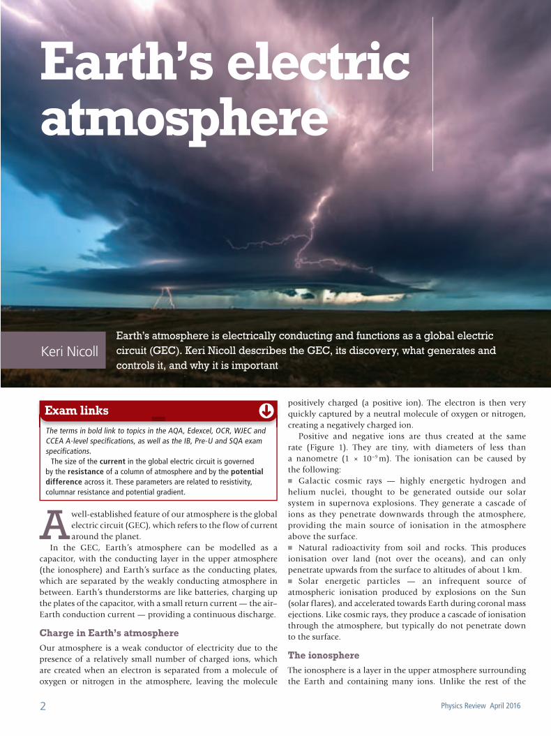
A well-established feature of our atmosphere is the global electric circuit (GEC), which refers to the flow of current around the planet.

In the GEC, Earth’s atmosphere can be modelled as a capacitor, with the conducting layer in the upper atmosphere (the ionosphere) and Earth’s surface as the conducting plates, which are separated by the weakly conducting atmosphere in between. Earth’s thunderstorms are like batteries, charging up the plates of the capacitor, with a small return current — the air–Earth conduction current — providing a continuous discharge.

Charge in Earth’s atmosphereOur atmosphere is a weak conductor of electricity due to the presence of a relatively small number of charged ions, which are created when an electron is separated from a molecule of oxygen or nitrogen in the atmosphere, leaving the molecule

positively charged (a positive ion). The electron is then very quickly captured by a neutral molecule of oxygen or nitrogen, creating a negatively charged ion.

Positive and negative ions are thus created at the same rate (Figure 1). They are tiny, with diameters of less than a nanometre (1 × 10−9 m). The ionisation can be caused by the following:

Galactic cosmic rays — highly energetic hydrogen and helium nuclei, thought to be generated outside our solar system in supernova explosions. They generate a cascade of ions as they penetrate downwards through the atmosphere, providing the main source of ionisation in the atmosphere above the surface.

Natural radioactivity from soil and rocks. This produces ionisation over land (not over the oceans), and can only penetrate upwards from the surface to altitudes of about 1 km.

Solar energetic particles — an infrequent source of atmospheric ionisation produced by explosions on the Sun (solar flares), and accelerated towards Earth during coronal mass ejections. Like cosmic rays, they produce a cascade of ionisation through the atmosphere, but typically do not penetrate down to the surface.

The ionosphereThe ionosphere is a layer in the upper atmosphere surrounding the Earth and containing many ions. Unlike the rest of the

Earth’s electric atmosphere

Earth’s atmosphere is electrically conducting and functions as a global electric circuit (GEC). Keri Nicoll describes the GEC, its discovery, what generates and controls it, and why it is important

Keri Nicoll

The terms in bold link to topics in the AQA, Edexcel, OCR, WJEC and CCEA A-level specifications, as well as the IB, Pre-U and SQA exam specifications.

The size of the current in the global electric circuit is governed by the resistance of a column of atmosphere and by the potential difference across it. These parameters are related to resistivity, columnar resistance and potential gradient.

Exam links

6233_PhysRev_25_4_Press2.indd 2 24/02/2016 10:23

3www.hoddereducation.co.uk/physicsreview

atmosphere, the ionosphere is a good conductor of electricity as it contains so many positive ions and free electrons.

UV radiation and X-rays from the Sun and high-energy particles (cosmic rays) from space continually knock electrons off the molecules of nitrogen and oxygen in the upper atmosphere, forming positive ions and free electrons. Free electrons can survive in the ionosphere because they rarely collide with the molecules and ions as these particles are so far apart in the very low-density atmosphere 60 km above Earth’s surface.

ThunderstormsThunderstorms are generated as a result of rapid upward movement of warm, moist air. Therefore, they are more typically found around the equator — i.e. Africa, South America and Southeast Asia. Measurements from satellites and ground-based lightning location/detection networks have shown that there are approximately 1000 thunderstorms active around the world at any one time (see references and further reading).

Each storm separates positive and negative charge. Positive charge is typically transferred towards the storm top and negative charge accumulates towards the bottom. Positive charge in the storm top flows upwards into the ionosphere, causing it to gain a net positive charge. At the same time, negative charge from the base of the storm is transferred down to Earth’s surface in lightning and negatively charged rain. Thus thunderstorms

actively transport charge, generating a large potential difference (voltage) between the ionosphere and Earth’s surface.

Measurements from aircraft flying in the region above storms have found that each one of those thunderstorms produces an upward positive current to the ionosphere, I

storm, of about 0.8 A. We can thus calculate the total upward current, Iup, from the number of global thunderstorms, Nstorm:

Iup = Nstorm × Istorm = 1000 × 0.8 A = 800 A (1)

If the global thunderstorm generator was suddenly switched off, and all thunderstorms stopped, the ionosphere would slowly discharge. The hypothetical discharge time is about 15 minutes.

Global current The potential difference between the ionosphere and Earth’s surface is approximately 250 kV (2.5 × 105 V). This very large potential difference means that the charged ions in the atmosphere will move and thus produce a vertical current. This is similar to electrons in a wire moving when connected to a voltage source, such as a battery. This vertical current flows globally in fair-weather regions (where there are no storms), between the ionosphere and the surface. Since measurements have never shown a complete absence of fair-weather current for any length of time it can be assumed that global thunderstorms are continuously generating current.

This framework of charge separation in thunderstorms and return current flow in fair-weather regions is known as the global electric circuit (GEC). The GEC is shown schematically in Figure 2 and Table 1 lists some of its key parameters.

Figure 1 Schematic representation of ionisation in Earth’s atmosphere

(1) (2) (3)

neutral molecule

ionising particle

++

negative ion

++

neutral molecule

electron

positive ion

+1

–1

++

++

Figure 2 (a) Schematic diagram of the global electric circuit (GEC). Red arrows denote the direction of positive charge flow. (b) Simple model of the GEC, where the battery symbol represents the global thunderstorm generator

ionosphere

Earth’s surface Earth’s surface

ionosphere

cosmic rays

Jc

JcIstorm

Vl

RcRcionisation

precipitationradongas

disturbedweatherregion

fair-weatherregion

+ + +

++

+

+ +

+

– – – –

–

– –

–

–

(a) (b)

+

–

Table 1 Atmospheric electrical and GEC parameters

Parameter Symbol Typical value

Ionospheric potential (potential difference between surface and ionosphere)

Vi 250 kV (2.5 × 105 V)

Air–Earth conduction current density

Jc 1–2 × 10−12 A m−2

Columnar resistance Rc 200 × 1015 Ω m2

Potential gradient at Earth’s surface

PG 100 V m−1

6233_PhysRev_25_4_Press2.indd 3 24/02/2016 10:23

4 Physics Review April 2016

Boxes 1 and 2 show how the parameters in Table 1 are related to the simple circuit model in Figure 2b.

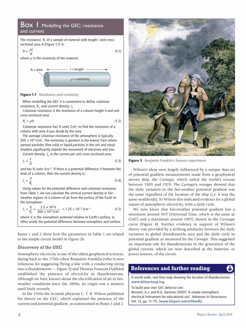
Discovery of the GECAtmospheric electricity is one of the oldest geophysical sciences, dating back to the 1750s when Benjamin Franklin (who is now infamous for suggesting flying a kite with a conducting string into a thunderstorm — Figure 3) and Thomas-François Dalibard established the presence of electricity in thunderstorms. Although we have known about the electrification of air in fair-weather conditions since the 1800s, its origin was a mystery until fairly recently.

In the 1920s the Scottish physicist C. T. R. Wilson published his theory on the GEC, which explained the presence of the current and potential gradient as summarised in Boxes 1 and 2.

A world-wide, real-time map showing the location of thunderstorms:www.blitzortung.org

To build your own GEC detector see:Bennett, A.J. and R.G. Harrison (2007) ‘A simple atmospheric electrical instrument for educational use’, Advances in Geoscience, Vol. 13, pp. 11–15. (www.tinyurl.com/nl5bw9k)

References and further reading References and further reading

Figure 3 Benjamin Franklin’s famous experiment

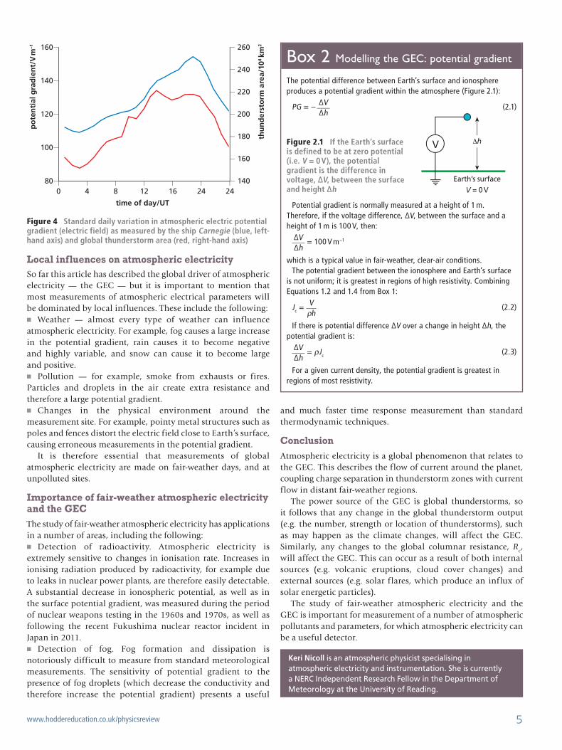
Wilson’s ideas were largely influenced by a unique data set of potential gradient measurements made from a geophysical survey ship, the Carnegie, which sailed the world’s oceans between 1909 and 1929. The Carnegie’s voyages showed that the daily variation in the fair-weather potential gradient was the same regardless of the location of the ship (i.e. it was the same worldwide). To Wilson this indicated evidence for a global nature of atmospheric electricity, with a daily cycle.

We now know that fair-weather potential gradient has a minimum around 3UT (Universal Time, which is the same as GMT) and a maximum around 19UT, shown in the Carnegie curve (Figure 4). Further evidence in support of Wilson’s theory was provided by a striking similarity between the daily variation in global thunderstorm area and the daily cycle in potential gradient as measured by the Carnegie. This suggested an important role for thunderstorms in the generation of the global current, which are now described as the batteries, or power sources, of the circuit.

Box 1 Modelling the GEC: resistance and current

The resistance, R, of a sample of material with length l and cross-sectional area A (Figure 1.1) is:

R = ρlA

(1.1)

where ρ is the resistivity of the material.

A = area l = length

= resistivityρ

Figure 1.1 Resistance and resistivity

When modelling the GEC it is convenient to define columnar resistance, Rc, and current density, Jc.

Columnar resistance is the resistance of a column height h and unit cross-sectional area:

Rc = ρh (1.2)

Columnar resistance has SI units Ω m2; to find the resistance of a column with area A you divide by the area.

The average columnar resistance of the atmosphere is typically 200 × 1015 Ω m2. The resistivity is greatest in the lowest 5 km where aerosol particles (fine solid or liquid particles in the air) and cloud droplets significantly impede the movement of electrons and ions.

Current density, Jc, is the current per unit cross-sectional area:

Jc = IA

(1.3)

and has SI units A m−2. If there is a potential difference V between the ends of a column, then the current density is:

Jc = VRc

(1.4)

Using values for the potential difference and columnar resistance from Table 1, we can calculate the vertical current density in fair-weather regions in a column of air from the surface of the Earth to the ionosphere:

Jc = VI

Rc

= 2.5 × 105 V200 × 1015 Ω m2

= 1.25 × 10−12 A m−2 (1.5)

where VI is the ionospheric potential relative to Earth’s surface, in other words the potential difference between ionosphere and surface.

6233_PhysRev_25_4_Press2.indd 4 24/02/2016 10:23

5www.hoddereducation.co.uk/physicsreview

Keri Nicoll is an atmospheric physicist specialising in atmospheric electricity and instrumentation. She is currently a NERC Independent Research Fellow in the Department of Meteorology at the University of Reading.

Figure 4 Standard daily variation in atmospheric electric potential gradient (electric field) as measured by the ship Carnegie (blue, left-hand axis) and global thunderstorm area (red, right-hand axis)

time of day/UT

po

ten

tial

gra

die

nt/

V m

–1

thu

nd

erst

orm

are

a/10

4 km

2

0 4 8 12 16 24 2480

100

120

140

160

140

160

180

200

220

240

260

Local influences on atmospheric electricitySo far this article has described the global driver of atmospheric electricity — the GEC — but it is important to mention that most measurements of atmospheric electrical parameters will be dominated by local influences. These include the following:

Weather — almost every type of weather can influence atmospheric electricity. For example, fog causes a large increase in the potential gradient, rain causes it to become negative and highly variable, and snow can cause it to become large and positive.

Pollution — for example, smoke from exhausts or fires. Particles and droplets in the air create extra resistance and therefore a large potential gradient.

Changes in the physical environment around the measurement site. For example, pointy metal structures such as poles and fences distort the electric field close to Earth’s surface, causing erroneous measurements in the potential gradient.

It is therefore essential that measurements of global atmospheric electricity are made on fair-weather days, and at unpolluted sites.

Importance of fair-weather atmospheric electricity and the GECThe study of fair-weather atmospheric electricity has applications in a number of areas, including the following:

Detection of radioactivity. Atmospheric electricity is extremely sensitive to changes in ionisation rate. Increases in ionising radiation produced by radioactivity, for example due to leaks in nuclear power plants, are therefore easily detectable. A substantial decrease in ionospheric potential, as well as in the surface potential gradient, was measured during the period of nuclear weapons testing in the 1960s and 1970s, as well as following the recent Fukushima nuclear reactor incident in Japan in 2011.

Detection of fog. Fog formation and dissipation is notoriously difficult to measure from standard meteorological measurements. The sensitivity of potential gradient to the presence of fog droplets (which decrease the conductivity and therefore increase the potential gradient) presents a useful

and much faster time response measurement than standard thermodynamic techniques.

ConclusionAtmospheric electricity is a global phenomenon that relates to the GEC. This describes the flow of current around the planet, coupling charge separation in thunderstorm zones with current flow in distant fair-weather regions.

The power source of the GEC is global thunderstorms, so it follows that any change in the global thunderstorm output (e.g. the number, strength or location of thunderstorms), such as may happen as the climate changes, will affect the GEC. Similarly, any changes to the global columnar resistance, R

c, will affect the GEC. This can occur as a result of both internal sources (e.g. volcanic eruptions, cloud cover changes) and external sources (e.g. solar flares, which produce an influx of solar energetic particles).

The study of fair-weather atmospheric electricity and the GEC is important for measurement of a number of atmospheric pollutants and parameters, for which atmospheric electricity can be a useful detector.

Box 2 Modelling the GEC: potential gradient

The potential difference between Earth’s surface and ionosphere produces a potential gradient within the atmosphere (Figure 2.1):

PG = − ΔVΔh

(2.1)

Figure 2.1 If the Earth’s surface is defined to be at zero potential (i.e. V = 0 V), the potential gradient is the difference in voltage, ΔV, between the surface and height Δh

Potential gradient is normally measured at a height of 1 m. Therefore, if the voltage difference, ΔV, between the surface and a height of 1 m is 100 V, then:

ΔVΔh

= 100 V m−1

which is a typical value in fair-weather, clear-air conditions. The potential gradient between the ionosphere and Earth’s surface

is not uniform; it is greatest in regions of high resistivity. Combining Equations 1.2 and 1.4 from Box 1:

Jc = Vρh

(2.2)

If there is potential difference ΔV over a change in height Δh, the potential gradient is:

ΔVΔh

= ρJc (2.3)

For a given current density, the potential gradient is greatest in regions of most resistivity.

Δh

V = 0 VEarth’s surface

V

6233_PhysRev_25_4_Press2.indd 5 24/02/2016 10:23