Earth and Planetary Science Letters 333–334 (2012) 9–20

Contents lists available at SciVerse ScienceDirect

Earth and Planetary Science Letters

0012-82

http://d

n Corr

Katherin

Austin,

E-m

ksoderlu

aurnou@

journal homepage: www.elsevier.com/locate/epsl

The influence of magnetic fields in planetary dynamo models

Krista M. Soderlund a,n, Eric M. King b, Jonathan M. Aurnou a

a Department of Earth and Space Sciences, University of California, Los Angeles, CA 90095, USAb Department of Earth and Planetary Science, University of California, Berkeley, CA 94720, USA

a r t i c l e i n f o

Article history:

Received 7 November 2011

Received in revised form

27 March 2012

Accepted 29 March 2012

Editor: T. SpohnPr¼1; magnetic Prandtl numbers up to Pm¼5; Ekman numbers in the range 10�3

ZEZ10�5; and

Keywords:

core convection

geodynamo

planetary dynamos

dynamo models

rotating convection models

1X/$ - see front matter & 2012 Elsevier B.V.

x.doi.org/10.1016/j.epsl.2012.03.038

esponding author. Present address: Institut

e G. Jackson School of Geosciences, The Un

TX 78758, USA. Tel.: þ1 218 349 3006; fax: þ

ail addresses: krista@ig.utexas.edu,

nd@gmail.com (K.M. Soderlund), eric.king@b

ucla.edu (J.M. Aurnou).

a b s t r a c t

The magnetic fields of planets and stars are thought to play an important role in the fluid motions

responsible for their field generation, as magnetic energy is ultimately derived from kinetic energy. We

investigate the influence of magnetic fields on convective dynamo models by contrasting them with

non-magnetic, but otherwise identical, simulations. This survey considers models with Prandtl number

Rayleigh numbers from near onset to more than 1000 times critical.

Two major points are addressed in this letter. First, we find that the characteristics of convection,

including convective flow structures and speeds as well as heat transfer efficiency, are not strongly

affected by the presence of magnetic fields in most of our models. While Lorentz forces must alter the

flow to limit the amplitude of magnetic field growth, we find that dynamo action does not necessitate a

significant change to the overall flow field. By directly calculating the forces in each of our simulations,

we show that the traditionally defined Elsasser number, Li , overestimates the role of the Lorentz force

in dynamos. The Coriolis force remains greater than the Lorentz force even in cases with LiC100,

explaining the persistence of columnar flows in Li41 dynamo simulations. We argue that a dynamic

Elsasser number, Ld , better represents the Lorentz to Coriolis force ratio. By applying the Ld

parametrization to planetary settings, we predict that the convective dynamics (excluding zonal flows)

in planetary interiors are only weakly influenced by their large-scale magnetic fields.

The second major point addressed here is the observed transition between dynamos with dipolar

and multipolar magnetic fields. We find that the breakdown of dipolar field generation is due to the

degradation of helicity in the flow. This helicity change does not coincide with the destruction of

columnar convection and is not strongly influenced by the presence of magnetic fields. Force

calculations suggest that this transition may be related to a competition between inertial and viscous

forces. If viscosity is indeed important for large-scale field generation, such moderate Ekman number

models may not adequately simulate the dynamics of planetary dynamos, where viscous effects are

expected to be negligible.

& 2012 Elsevier B.V. All rights reserved.

1. Introduction

Magnetic fields are common throughout the solar system;intrinsic magnetic fields have been detected on the Sun, Mercury,Earth, the giant planets, and the Jovian satellite Ganymede(Connerney, 2007). Evidence of extinct dynamos is also observedon the Moon and Mars (Connerney, 2007). In addition, it isexpected that many extrasolar planets have magnetic fields

All rights reserved.

e for Geophysics, John A. &

iversity of Texas at Austin,

1 512 471 8844.

erkeley.edu (E.M. King),

(e.g., Gaidos et al., 2010). Planetary magnetic fields result fromdynamo action thought to be driven by convection in electricallyconducting fluid regions (e.g., Jones, 2011) and, therefore, arelinked to the planets’ internal dynamics. Convection in thesesystems is subject to Coriolis forces resulting from planetaryrotation. In electrically conducting fluids, these flows can beunstable to dynamo action. Lorentz forces then arise, via Lenz’slaw, that act to equilibrate magnetic field growth.

Insight into the forces that govern the fluid dynamics ofplanetary interiors can be gained through numerical modeling:non-magnetic rotating convection models investigate the influ-ence of rotation on convection, and planetary dynamo modelsincorporate the additional back reaction of the magnetic fields onthe fluid motions from which they arise.

The flows in non-magnetic rapidly rotating convection areorganized by the Coriolis force into axial columns (e.g., Grooms

K.M. Soderlund et al. / Earth and Planetary Science Letters 333–334 (2012) 9–2010

et al., 2010; Olson, 2011; King and Aurnou, 2012). Under theextreme influence of rotation, the dominant force balance isgeostrophic—a balance between the Coriolis force and the pres-sure gradient. Geostrophic flows are described by the Taylor–Proudman constraint, which predicts that fluid motions shouldnot vary strongly in the direction of the rotation axis (e.g., Tritton,1998). Furthermore, linear asymptotic analyses predict that theazimuthal wavenumber of these columns varies as m¼OðE�1=3

Þ

as E-0 (Roberts, 1968; Jones et al., 2000; Dormy et al., 2004).Here, m is non-dimensionalized by the shell thickness and theEkman number, E, characterizes the ratio of viscous to Coriolis

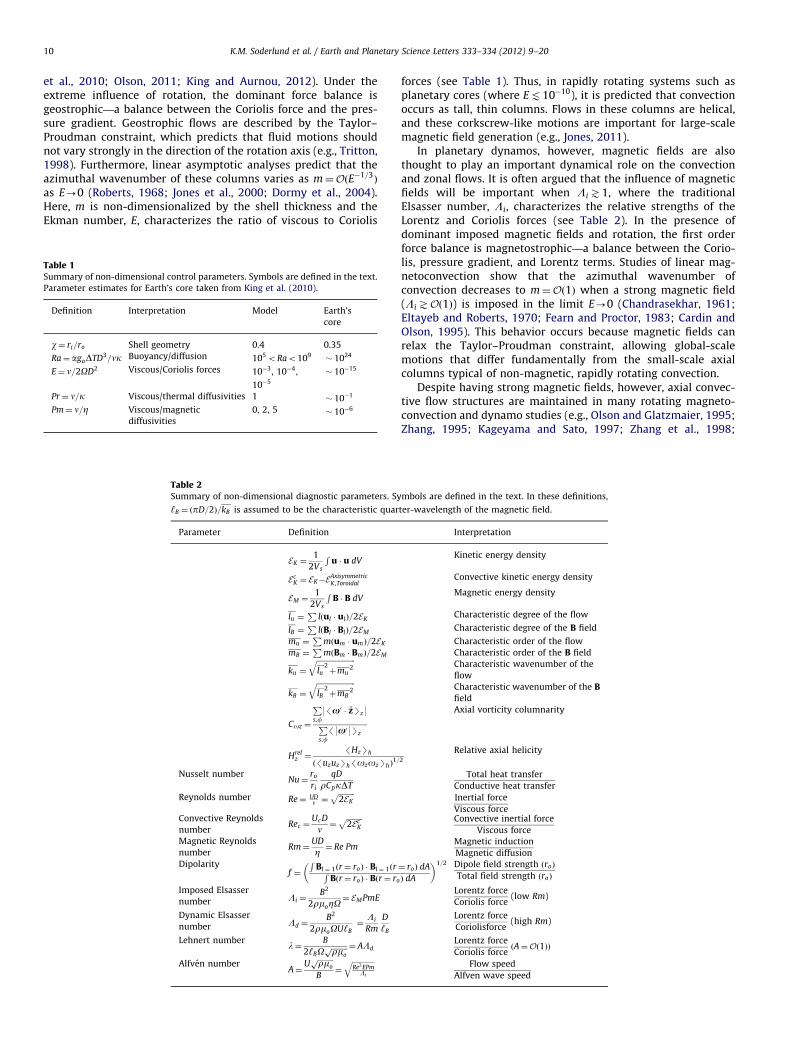
Table 1Summary of non-dimensional control parameters. Symbols are defined in the text.

Parameter estimates for Earth’s core taken from King et al. (2010).

Definition Interpretation Model Earth’s

core

w¼ ri=ro Shell geometry 0.4 0.35

Ra¼ agoDTD3=nk Buoyancy/diffusion 105 oRao109� 1024

E¼ n=2OD2 Viscous/Coriolis forces 10�3, 10�4,

10�5

� 10�15

Pr ¼ n=k Viscous/thermal diffusivities 1 � 10�1

Pm¼ n=Z Viscous/magnetic

diffusivities

0, 2, 5 � 10�6

Table 2Summary of non-dimensional diagnostic parameters. Sy

‘B ¼ ðpD=2Þ=kB is assumed to be the characteristic quar

Parameter Definition

EK ¼1

2Vs

Ru � u dV

EcK ¼ EK�EAxisymmetric

K ,Toroidal

EM ¼1

2Vs

RB � B dV

lu ¼P

lðul � ulÞ=2EK

lB ¼P

lðBl � BlÞ=2EM

mu ¼P

mðum � umÞ=2EK

mB ¼P

mðBm � BmÞ=2EM

ku ¼

ffiffiffiffiffiffiffiffiffiffiffiffiffiffiffiffiffiffiffiffiffilu

2þmu

2

q

kB ¼

ffiffiffiffiffiffiffiffiffiffiffiffiffiffiffiffiffiffiffiffiffilB

2þmB

2

q

Coz ¼

Ps,f

9/x0 � zSz9

Ps,f

/9x09Sz

Hrelz ¼

/HzSh

ð/uzuzSh/ozozShÞ1=

Nusselt numberNu¼

ro

ri

qD

rCpkDT

Reynolds number Re¼ UDn ¼

ffiffiffiffiffiffiffiffiffi2EK

p

Convective Reynolds

numberRec ¼

UcD

n ¼ffiffiffiffiffiffiffiffiffi2Ec

K

pMagnetic Reynolds

numberRm¼

UD

Z ¼ Re Pm

Dipolarityf ¼

RBl ¼ 1ðr¼ roÞ � Bl ¼ 1ðrR

Bðr¼ roÞ � Bðr¼ ro

�

Imposed Elsasser

number Li ¼B2

2rmoZO¼ EMPmE

Dynamic Elsasser

number Ld ¼B2

2rmoOU‘B¼

Li

Rm

D

‘B

Lehnert numberl¼

B

2‘BOffiffiffiffiffiffiffiffiffirmop ¼ ALd

Alfven numberA¼

Uffiffiffiffiffiffiffiffiffirmop

B¼

ffiffiffiffiffiffiffiffiffiffiffiffiRe2 EPm

Li

q

forces (see Table 1). Thus, in rapidly rotating systems such asplanetary cores (where Et10�10), it is predicted that convectionoccurs as tall, thin columns. Flows in these columns are helical,and these corkscrew-like motions are important for large-scalemagnetic field generation (e.g., Jones, 2011).

In planetary dynamos, however, magnetic fields are alsothought to play an important dynamical role on the convectionand zonal flows. It is often argued that the influence of magneticfields will be important when Li\1, where the traditionalElsasser number, Li, characterizes the relative strengths of theLorentz and Coriolis forces (see Table 2). In the presence ofdominant imposed magnetic fields and rotation, the first orderforce balance is magnetostrophic—a balance between the Corio-lis, pressure gradient, and Lorentz terms. Studies of linear mag-netoconvection show that the azimuthal wavenumber ofconvection decreases to m¼Oð1Þ when a strong magnetic field(Li\Oð1Þ) is imposed in the limit E-0 (Chandrasekhar, 1961;Eltayeb and Roberts, 1970; Fearn and Proctor, 1983; Cardin andOlson, 1995). This behavior occurs because magnetic fields canrelax the Taylor–Proudman constraint, allowing global-scalemotions that differ fundamentally from the small-scale axialcolumns typical of non-magnetic, rapidly rotating convection.

Despite having strong magnetic fields, however, axial convec-tive flow structures are maintained in many rotating magneto-convection and dynamo studies (e.g., Olson and Glatzmaier, 1995;Zhang, 1995; Kageyama and Sato, 1997; Zhang et al., 1998;

mbols are defined in the text. In these definitions,

ter-wavelength of the magnetic field.

Interpretation

Kinetic energy density

Convective kinetic energy density

Magnetic energy density

Characteristic degree of the flow

Characteristic degree of the B field

Characteristic order of the flow

Characteristic order of the B field

Characteristic wavenumber of the

flow

Characteristic wavenumber of the Bfield

Axial vorticity columnarity

2

Relative axial helicity

Total heat transfer

Conductive heat transfer

Inertial force

Viscous forceConvective inertial force

Viscous forceMagnetic induction

Magnetic diffusion

¼ roÞ dA

Þ dA

�1=2 Dipole field strength ðroÞ

Total field strength ðroÞ

Lorentz force

Coriolis force(low Rm)

Lorentz force

Coriolisforce(high Rm)

Lorentz force

Coriolis forceðA¼Oð1ÞÞ

Flow speed

Alfven wave speed

K.M. Soderlund et al. / Earth and Planetary Science Letters 333–334 (2012) 9–20 11

Christensen et al., 1999; Zhang and Schubert, 2000; Jones, 2007;Jault, 2008; Busse and Simitev, 2011). Further, King et al. (2010)have shown that heat transfer scaling laws from non-magneticplanar convection also apply to planetary dynamo models,regardless of magnetic field strength. These results imply thatthe traditional force balance argument from linear analysis usingthe Elsasser number Li may not be an adequate measure of thedynamical influence of the Lorentz force in convection systems.Alternate characterizations of the Lorentz to Coriolis force ratiomust therefore be considered.

Here, we contrast dynamo models with non-magnetic, butotherwise identical, rotating convection models to quantify theinfluence of magnetic fields on convective dynamics. Whilecomparisons between dynamo and non-magnetic simulationshave been conducted (e.g., Christensen et al., 1999; Grote andBusse, 2001; Aubert, 2005), these studies are typically limited toconvection less than 40 times critical and dipolar magnetic fieldgeometries. Our survey is complementary to these earlier studiesas it extends the comparison to convection more than 1000 timescritical, considers both dipolar and multipolar magnetic fields,and makes no assumptions of azimuthal symmetries.

We measure the strengths and structures of magnetic fieldsand fluid motions, as well as heat transfer efficiency. We focus on,in order of priority, (i) the effect of the presence of magnetic fieldson convection, (ii) the effect of varying convective vigor, and (iii)the effect of varying the rotation rate. In Section 2, we detail themodel and methods. Behavioral regimes found in our models withfixed E¼ 10�4 are discussed in Section 3, and we analyze para-metrizations of the magnetic field influence in Section 4. InSection 5, we examine the transition from dipolar to multipolardynamos. Section 6 investigates the influence of varying theEkman number, while Section 7 applies our results to planetarycores. Our conclusions are given in Section 8.

2. Numerical model

We use the numerical model MagIC 3.38 (Wicht, 2002;Christensen and Wicht, 2007), which is based on the originalpseudospectral code of Glatzmaier (1984). This model simulatesthree-dimensional, time-dependent thermal convection of a Bous-sinesq fluid in a spherical shell rotating with constant angularvelocity Oz. We conduct two sets of simulations: (i) non-magneticrotating convection models which employ an electrically insulat-ing fluid and (ii) dynamo models which employ an electricallyconducting fluid. The shell geometry is defined by the ratio of theinner to outer shell radii, w¼ ri=ro ¼ 0:4. The shell boundaries areisothermal with an imposed (superadiabatic) temperature con-trast DT between the inner and outer boundaries. The mechanicalboundary conditions are impenetrable and no-slip. Gravity varieslinearly with spherical radius. The region exterior to the fluid shellis electrically insulating, and the electrical conductivity of the rigidinner sphere is chosen to be the same as that of the convectingfluid region.

The dimensionless governing equations for this system are

E@u

@tþu � ru�r2u

� �þ z � uþ

1

2rp¼

RaE

Pr

r

roTþ

1

2Pmðr � BÞ � B,

ð1Þ

@B

@t¼r � ðu� BÞþ

1

Pmr2B, ð2Þ

@T

@tþu � rT ¼

1

Prr

2T , ð3Þ

r � u¼ 0, r � B¼ 0, ð4Þ

where u is the velocity vector, B is the magnetic induction, T isthe temperature, and p is the non-hydrostatic pressure. Wemake use of typical non-dimensionalizations used in the plane-tary dynamo literature: shell thickness D¼ ro�ri as length scale;DT as temperature scale; tn �D2=n as time scale; rnO aspressure scale; n=D as velocity scale such that the non-dimen-sional globally averaged rms flow velocity is equal to theReynolds number Re¼UD=n; and

ffiffiffiffiffiffiffiffiffiffiffiffiffiffiffiffiffiffi2rmoZO

pas magnetic induc-

tion scale such that the square of the non-dimensional globallyaveraged rms magnetic field strength is equal to the tradition-ally defined Elsasser number Li ¼ B2= 2rmoZO. In these defini-tions, r is the density, n is the kinematic viscosity, k is thethermal diffusivity, Z is the magnetic diffusivity, mo is themagnetic permeability of free space, and a is the thermalexpansion coefficient.

The non-dimensional control parameters are the shell geome-try w¼ ri=ro, the Rayleigh number Ra¼ agoDTD3=nk, the Ekmannumber E¼ n=2OD2, the Prandtl number Pr¼ n=k, and the mag-netic Prandtl number Pm¼ n=Z. The Rayleigh number charac-terizes the ratio of buoyancy to diffusion. The Ekman numbercharacterizes the ratio of viscous to Coriolis forces. The Prandtlnumbers Pr and Pm characterize the ratio of viscous to thermaland magnetic diffusivities, respectively. The control parameterdefinitions are summarized in Table 1; the diagnostic parametersare defined in Table 2.

Our suite of simulations consists of 36 planetary dynamomodels and 30 non-magnetic rotating convection models. Thissurvey considers Prandtl number Pr¼1, magnetic Prandtl num-bers up to Pm¼5, Ekman numbers in the range 10�3

ZEZ10�5,and Rayleigh numbers from near onset to more than 1000 timescritical. The critical Rayleigh number, Rac, denotes the onset ofconvection. Here, we use the inferred scaling Rac ¼ 3:5E�4=3 fromKing et al. (2010). The Rayleigh numbers then fall in the range1:9Rac rRar1125Rac . This dataset, given in SupplementaryTables 4 and 5, is among the broadest surveys of supercriticalitymade to date.

The value of Pm is chosen such that the magnetic Reynoldsnumber Rm¼ Re Pm\102, a necessary condition for dynamoaction. For most of our simulations, the parameters are fixed tothe following values, which are commonly used in the currentplanetary dynamo literature: E¼ 10�4, Pr¼1, and Pm¼ ½0;2�.Dynamo models with similar parameters values have been arguedto generate Earth-like magnetic field morphologies (Christensenet al., 2010; Christensen, 2011).

The largest numerical grid uses 213 spherical harmonic modes,65 radial levels in the outer shell, and 17 radial levels in the innercore. No azimuthal symmetries are employed. Dynamo modelsare initialized using the results of prior dynamo simulations. Non-magnetic models are initialized by turning off the magnetic fieldof the associated dynamo model, similar to Zhang et al. (1998)among others. Some studies have found initial conditions to beimportant (e.g., Simitev and Busse, 2009; Sreenivasan and Jones,2011; Dormy, 2011), owing to bistable dynamo states. Thus, wetest for bistability by comparing results obtained with differentinitial conditions for a limited number of cases and find nosignificant differences in time-averaged behaviors. Once theinitial transient behavior has subsided, time-averaged propertiesfor cases with Rar11Rac are averaged over at least tO � tn=pE41500 rotations, cases with 11Rac oRar56Rac are averaged overat least 500 rotations, and all other cases are averaged over atleast 30 rotations.

Hyperdiffusion is used in five of our 66 simulations. It is appliedin our most supercritical models (RaZ562Rac for E¼ 10�4;Ra¼ 12:5Rac for E¼ 10�5) to increase numerical stability by damp-ing the small-scale components of the velocity, thermal, and mag-netic fields. In these models, the viscous, thermal, and magnetic

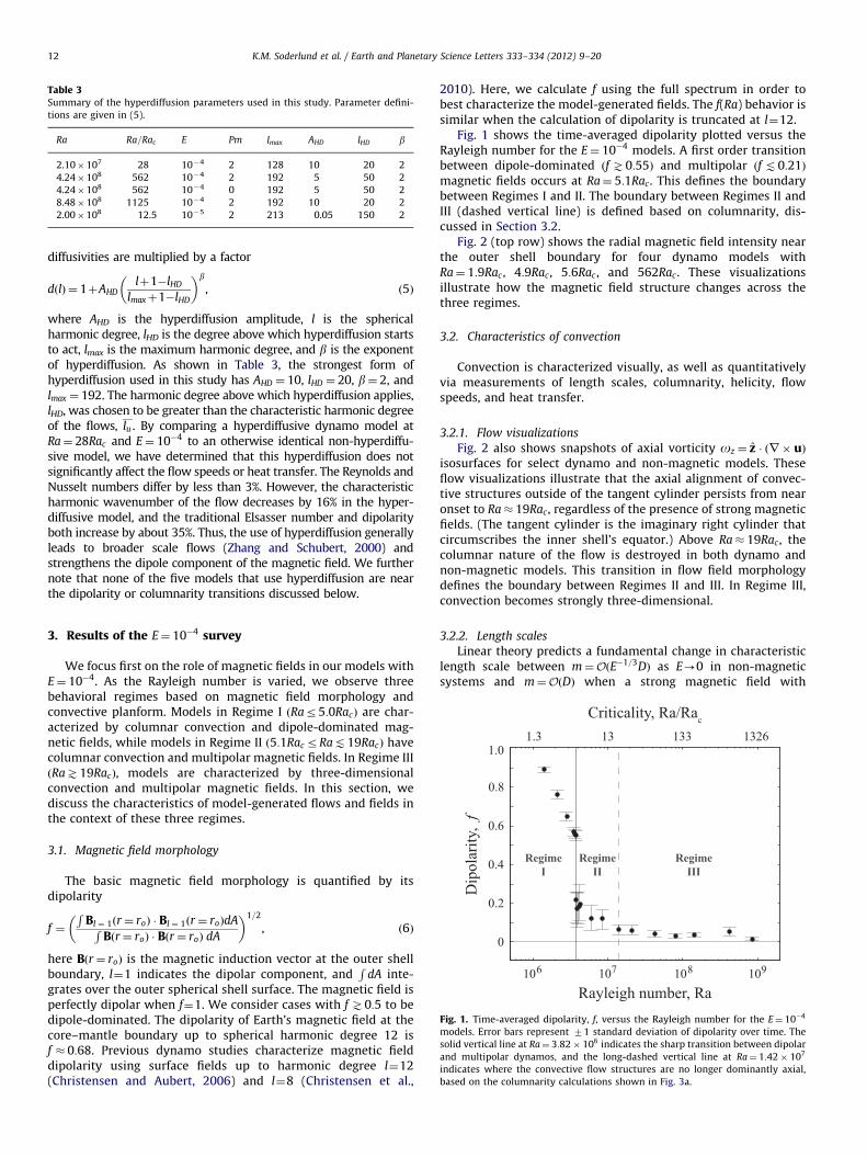
Table 3Summary of the hyperdiffusion parameters used in this study. Parameter defini-

tions are given in (5).

Ra Ra=Rac E Pm lmax AHD lHD b

2.10�107 28 10�4 2 128 10 20 2

4.24�108 562 10�4 2 192 5 50 2

4.24�108 562 10�4 0 192 5 50 2

8.48�108 1125 10�4 2 192 10 20 2

2.00�108 12.5 10�5 2 213 0.05 150 2

K.M. Soderlund et al. / Earth and Planetary Science Letters 333–334 (2012) 9–2012

diffusivities are multiplied by a factor

dðlÞ ¼ 1þAHDlþ1�lHD

lmaxþ1�lHD

� �b

, ð5Þ

where AHD is the hyperdiffusion amplitude, l is the sphericalharmonic degree, lHD is the degree above which hyperdiffusion startsto act, lmax is the maximum harmonic degree, and b is the exponentof hyperdiffusion. As shown in Table 3, the strongest form ofhyperdiffusion used in this study has AHD ¼ 10, lHD ¼ 20, b¼ 2, andlmax ¼ 192. The harmonic degree above which hyperdiffusion applies,lHD, was chosen to be greater than the characteristic harmonic degreeof the flows, lu . By comparing a hyperdiffusive dynamo model atRa¼ 28Rac and E¼ 10�4 to an otherwise identical non-hyperdiffu-sive model, we have determined that this hyperdiffusion does notsignificantly affect the flow speeds or heat transfer. The Reynolds andNusselt numbers differ by less than 3%. However, the characteristicharmonic wavenumber of the flow decreases by 16% in the hyper-diffusive model, and the traditional Elsasser number and dipolarityboth increase by about 35%. Thus, the use of hyperdiffusion generallyleads to broader scale flows (Zhang and Schubert, 2000) andstrengthens the dipole component of the magnetic field. We furthernote that none of the five models that use hyperdiffusion are nearthe dipolarity or columnarity transitions discussed below.

Fig. 1. Time-averaged dipolarity, f, versus the Rayleigh number for the E¼ 10�4

models. Error bars represent 71 standard deviation of dipolarity over time. The

solid vertical line at Ra¼ 3:82� 106 indicates the sharp transition between dipolar

and multipolar dynamos, and the long-dashed vertical line at Ra¼ 1:42� 107

indicates where the convective flow structures are no longer dominantly axial,

based on the columnarity calculations shown in Fig. 3a.

3. Results of the E¼ 10�4 survey

We focus first on the role of magnetic fields in our models withE¼ 10�4. As the Rayleigh number is varied, we observe threebehavioral regimes based on magnetic field morphology andconvective planform. Models in Regime I ðRar5:0RacÞ are char-acterized by columnar convection and dipole-dominated mag-netic fields, while models in Regime II ð5:1Rac rRat19RacÞ havecolumnar convection and multipolar magnetic fields. In Regime IIIðRa\19RacÞ, models are characterized by three-dimensionalconvection and multipolar magnetic fields. In this section, wediscuss the characteristics of model-generated flows and fields inthe context of these three regimes.

3.1. Magnetic field morphology

The basic magnetic field morphology is quantified by itsdipolarity

f ¼

RBl ¼ 1ðr¼ roÞ � Bl ¼ 1ðr¼ roÞdAR

Bðr¼ roÞ � Bðr¼ roÞ dA

� �1=2

, ð6Þ

here Bðr¼ roÞ is the magnetic induction vector at the outer shellboundary, l¼1 indicates the dipolar component, and

RdA inte-

grates over the outer spherical shell surface. The magnetic field isperfectly dipolar when f¼1. We consider cases with f \0:5 to bedipole-dominated. The dipolarity of Earth’s magnetic field at thecore–mantle boundary up to spherical harmonic degree 12 isf � 0:68. Previous dynamo studies characterize magnetic fielddipolarity using surface fields up to harmonic degree l¼12(Christensen and Aubert, 2006) and l¼8 (Christensen et al.,

2010). Here, we calculate f using the full spectrum in order tobest characterize the model-generated fields. The f(Ra) behavior issimilar when the calculation of dipolarity is truncated at l¼12.

Fig. 1 shows the time-averaged dipolarity plotted versus theRayleigh number for the E¼ 10�4 models. A first order transitionbetween dipole-dominated ðf \0:55Þ and multipolar ðf t0:21Þmagnetic fields occurs at Ra¼ 5:1Rac . This defines the boundarybetween Regimes I and II. The boundary between Regimes II andIII (dashed vertical line) is defined based on columnarity, dis-cussed in Section 3.2.

Fig. 2 (top row) shows the radial magnetic field intensity nearthe outer shell boundary for four dynamo models withRa¼ 1:9Rac , 4:9Rac , 5:6Rac , and 562Rac . These visualizationsillustrate how the magnetic field structure changes across thethree regimes.

3.2. Characteristics of convection

Convection is characterized visually, as well as quantitativelyvia measurements of length scales, columnarity, helicity, flowspeeds, and heat transfer.

3.2.1. Flow visualizations

Fig. 2 also shows snapshots of axial vorticity oz ¼ z � ðr � uÞisosurfaces for select dynamo and non-magnetic models. Theseflow visualizations illustrate that the axial alignment of convec-tive structures outside of the tangent cylinder persists from nearonset to Ra� 19Rac , regardless of the presence of strong magneticfields. (The tangent cylinder is the imaginary right cylinder thatcircumscribes the inner shell’s equator.) Above Ra� 19Rac , thecolumnar nature of the flow is destroyed in both dynamo andnon-magnetic models. This transition in flow field morphologydefines the boundary between Regimes II and III. In Regime III,convection becomes strongly three-dimensional.

3.2.2. Length scales

Linear theory predicts a fundamental change in characteristiclength scale between m¼OðE�1=3DÞ as E-0 in non-magneticsystems and m¼OðDÞ when a strong magnetic field with

Fig. 2. Instantaneous radial magnetic fields near the outer shell boundary (top row) and isosurfaces of instantaneous axial vorticity for select E¼ 10�4 dynamo (middle

row) and non-magnetic (bottom row) models. Purple (green) indicates radially outward (inward) directed magnetic fields. Red (blue) indicates cyclonic (anticyclonic)

vorticity. Each subplot has its own color scale. The inner yellow sphere represents the inner shell boundary. The outer boundary layer has been excluded for clarity. Below

each image is either the dipolarity, f, or the axial vorticity columnarity, Coz . (For interpretation of the references to color in this figure caption, the reader is referred to the

web version of this article.)

K.M. Soderlund et al. / Earth and Planetary Science Letters 333–334 (2012) 9–20 13

Li\Oð1Þ is imposed in the limit E-0 (Chandrasekhar, 1961).This prediction is tested by comparing the characteristic wave-numbers of the flow field in the dynamo and non-magneticmodels

ku ¼

ffiffiffiffiffiffiffiffiffiffiffiffiffiffiffiffiffiffiffiffilu

2þmu

2

q, ð7aÞ

where

lu ¼Xl ¼ lmax

l ¼ 0

lðul � ulÞ

2EKð7bÞ

and

mu ¼Xm ¼ mmax

m ¼ 0

mðum � umÞ

2EK, ð7cÞ

here ul is the velocity at spherical harmonic degree l, um is thevelocity at spherical harmonic order m, and EK is the kineticenergy. The time-averaged values, given in SupplementaryTable 6, show that the presence of dynamo-generated magneticfields alters the value of ku by at most 14% in comparison to theassociated non-magnetic cases. Thus, these dynamo models donot produce the fundamental change in length scale that lineartheory predicts.

3.2.3. Columnarity

We can also quantify the style of convection using axialvorticity measurements. Quasigeostrophic convection is domi-nated by axial, vortical columns that extend in z across the entireshell. We define ‘columnarity’ using a measure of the axialvariations of axial vorticity, oz, in the bulk fluid outside of the

tangent cylinder

Coz ¼

Ps,f9/x0 � zSz9P

s,f/9x09Sz

, ð8Þ

here /Sz indicates averages in the axial z direction, x0 indicatesvorticity calculated using only the non-axisymmetric velocityfield, and the summation occurs over the equatorial plane ðs,fÞ.Columnar convection has relatively large columnarity, Coz\0:5,because vorticity, x0, is dominated by its axial component, x0 � z.We consider cases with Coz\0:5 to be columnar, similar to ourconvention for f. Thus, we define the transition between RegimesII and III to occur where C � 0:5. Comparison of axial vorticityisosurfaces shows this convention to be an adequate proxy for thebreakdown of columnar convection.

Fig. 3a shows columnarity as a function of the Rayleigh numberfor the E¼ 10�4 models. The Coz values agree to within an averageof 4% between the dynamo and non-magnetic models, with amaximum difference of 14%. The presence of magnetic fields,therefore, does not change the basic planform of convection.

Columnar convection breaks down near Ra¼ 19Rac , whereCozo0:5 (Fig. 3a). King et al. (2009, 2010) argue that the break-down of columnar convection occurs when the thermal boundarylayer becomes thinner than the Ekman boundary layer. Wecalculate these boundary layer thicknesses and find that theyindeed cross at the transition between Regimes II and III.

This columnarity transition does not, however, coincide withthe magnetic field morphology transition at Ra¼ 5:1Rac . There-fore, columnar convection can generate both dipolar (Regime I)and multipolar (Regime II) magnetic fields. It is also worth noting

Fig. 3. (a) Instantaneous axial vorticity columnarity, Coz , (b) instantaneous relative axial helicity, 9Hrelz 9, (c) time-averaged convective flow speeds, Rec, and (d) time-

averaged heat transfer efficiency, Nu, as a function of the Rayleigh number for the E¼ 10�4 models. The dotted lines indicate classic scalings for non-rotating, non-magnetic

convection: (c) RecpRa1=2 and (d) NupRa2=7. In each plot, the solid and long-dashed vertical lines indicate transitions in dipolarity and columnarity, respectively, defined

in the Fig. 1 caption.

K.M. Soderlund et al. / Earth and Planetary Science Letters 333–334 (2012) 9–2014

that, in contrast to the sharp transition in dipolarity, Coz tends todecrease gradually with increased Rayleigh number such that afirst order transition does not occur.

3.2.4. Helicity

Helicity is common to rotating convection systems and isthought to be essential to large-scale magnetic field generation(e.g., Parker, 1955; Moffatt, 1978; Roberts, 2007). Helical flow isthe corkscrew-like motion produced by correlations betweenvelocity and vorticity fields. Here, we consider axial helicity,Hz ¼ uzoz. Relative axial helicity is defined as axial helicitynormalized by its maximum possible value

Hrelz ¼

/HzSh

ð/uzuzSh/ozozShÞ1=2

, ð9Þ

where /Sh is the volumetric average in each hemisphere exclud-ing boundary layers (e.g., Olson et al., 1999; Schmitz and Tilgner,2010, cf. Sreenivasan and Jones, 2011). Since axial helicity tendsto be anti-symmetric across the equator, we report the averagehelicity magnitude averaged over both hemispheres, 9Hrel

z 9.Fig. 3b shows calculations of relative axial helicity plotted

versus the Rayleigh number. Helicity is not appreciably sensitiveto the presence of magnetic fields in these models; our dynamoand non-magnetic simulations produce 9Hrel

z 9 values that typicallydiffer by less than 10%. Helicity is diminished by increasedthermal forcing (Ra). Regime I models exhibit strongly helicalflows with 9Hrel

z 9\0:4. Near the Regimes I and II boundary(3:8rRa=Rac r8:0), helicity drops off significantly. The three-dimensional flows in Regime III models are poorly correlated,such that 9Hrel

z 9t0:1.The degradation of helical flow occurs at lower Rayleigh

numbers than where columnar convection breaks down. This

implies that changes in axial vorticity are not responsible for thehelicity decrease. The breakdown of helicity is, however, coin-cident with the dipolarity transition in Fig. 1. We discuss this infurther detail in Section 5.

3.2.5. Convective flow speeds

Convective flow speeds are given by the convective Reynoldsnumber Rec ¼UcD=n, where Uc is the rms flow speed excludingthe axisymmetric zonal flow component. Zonal flows are weak inour models due to the no-slip boundaries; non-zonal flow speeds,Rec, and total flow speeds, Re, differ by than less than 13% in all ofour E¼ 10�4 models. This difference is maximum for the stronglysupercritical models where relatively strong zonal flows candevelop.

Fig. 3c plots the time-averaged convective Reynolds numberversus the Rayleigh number. The non-magnetic models have Rec

values that are on average 13% stronger than those of associateddynamos, with a maximum difference of 21%. This indicates thatflow speeds are reduced by the Lorentz force as kinetic energy istransferred to magnetic energy. Fig. 3c shows that the convectiveflow speeds, however, are more sensitive to thermal driving (Ra)than the presence of magnetic fields.

The dotted line in Fig. 3c shows the classic RepRa1=2 ‘free-fall’scaling law found in non-magnetic, non-rotating turbulent con-vection (e.g., Sano et al., 1989; Castaing et al., 1989; Siggia, 1994;Tilgner, 1996). Our data roughly follow this scaling in Regime III,which suggests that neither magnetic fields nor rotation stronglyinfluence these cases.

3.2.6. Heat transfer

Fig. 3d shows the time-averaged heat transfer behavior plottedversus the Rayleigh number. The Nusselt number, Nu, is the ratio

K.M. Soderlund et al. / Earth and Planetary Science Letters 333–334 (2012) 9–20 15

of total to conductive heat transfer

Nu¼ro

ri

qD

rCpkDT, ð10Þ

where q is the heat flux per unit area on the outer shell boundaryand Cp is the specific heat capacity. Between the dynamo and non-magnetic models, the Nusselt numbers agree to within an average of3%, with a maximum difference of 10%. In Regime I, the presence ofmagnetic fields tends to produce slightly larger radial length scales(see Supplementary Table 4) that transport heat more efficiently. InRegime III, magnetic fields weakly damp flow speeds (Fig. 3c),tending to reduce heat transport. Overall, the magnetic field has asecond order influence on heat transport in these models. The classicNupRa2=7 scaling law often found in non-magnetic, non-rotatingturbulent convection systems (e.g., Castaing et al., 1989; Glazieret al., 1999) is superimposed in Fig. 3d. A comparison of our dataagainst this scaling further supports our contention that inertiallydominated convection occurs in Regime III.

3.3. Force integrals

The competition between Lorentz (FL), Coriolis (FC), inertial (FI),and viscous (FV) forces can be quantified by comparing terms in themomentum equation. Toward this end, the forces are integratedover the entire spherical shell volume: F ¼

RV ðF

2r þF2

yþF 2fÞ

1=2 dV

where F is a generic force density. Boundary layers are included inthe integration, but their exclusion does not significantly affect theresults, with the exception of the viscous force integral where up to50% of the force is contained within the boundary layer.

Fig. 4 shows these force integral calculations and their ratiosfor all dynamo and non-magnetic models with E¼ 10�4. In bothsets of models, the Coriolis term dominates in Regimes I and II,indicating that these models are in quasigeostrophic balance,

Fig. 4. (a) and (c), respectively, plot instantaneous integrals of the rms Coriolis, Lorentz

and non-magnetic models. Ratios of the force integrals are shown in (b) and (d) for the

dashed vertical lines indicate transitions in dipolarity and columnarity, respectively, d

consistent with the prevalence of columnar convection withinthese regimes.

The Lorentz force is not a dominant influence on convectiondynamics in these models. The ratio of Lorentz to Coriolis forcesdoes not exceed 0.3 in Regimes I and II, while the ratio of Lorentzto inertial forces is less than 0.7 in Regimes II and III. Thissubdominance of the Lorentz force explains why our dynamoand rotating convection models exhibit similar behaviors. Insimilar models, it has been found that the Lorentz force isspatially intermittent (e.g., Sreenivasan and Jones, 2006; Aubertet al., 2008). So although the Lorentz force is globally subdomi-nant, it can be dynamically important in the sparse regions ofstrong magnetic field intensification.

3.4. Zonal flows

While we are primarily focused on the convective, non-zonaldynamics in this paper, we also note that a first order change inthe style of zonal flow occurs between dipolar and multipolardynamo models. Aubert (2005) shows that dipolar magnetic fieldsplay a critical role in the zonal flow power budget, yet we findthat the non-zonal convection tends not to be strongly sensitiveto magnetic fields in our E¼ 10�4 models. This difference inbehavior occurs because the pressure gradient term can balancethe Coriolis force in the full momentum equation, but is identi-cally zero in the axisymmetric azimuthal momentum equation. Asa result, the convective flows are quasigeostrophic, while thegeostrophic force balance cannot be established for the zonal flow(e.g., Roberts and Aurnou, 2011). The Lorentz force must thenbalance the Coriolis force in the zonal momentum equation whenthe inertial and viscous forces are weak. Consequently, this leadsto first order differences in zonal flows between the dynamo andassociated non-magnetic models.

, inertial, and viscous forces versus the Rayleigh number for the E¼ 10�4 dynamo

dynamo and non-magnetic models, respectively. In each plot, the solid and long-

efined in the Fig. 1 caption.

K.M. Soderlund et al. / Earth and Planetary Science Letters 333–334 (2012) 9–2016

4. Parametrization of magnetic field influence

In this section, we compare calculations and parametrizationsof the Lorentz to Coriolis force ratios in our E¼ 10�4 models.

4.1. Traditional Elsasser number

Following the developments of Christensen et al. (1999) andCardin et al. (2002), the ratio of the Lorentz force ðJ� B=rÞ toCoriolis force ð2X� uÞ is parametrized by the general form of theElsasser number

L¼JB

2rOU: ð11Þ

In order to estimate L using rms magnetic field strength B, thecurrent density J is characterized via either Ohm’s law

J¼ sðEþu� BÞ ð12Þ

(where s¼ 1=moZ is the electrical conductivity), or Ampere’s lawunder the MHD approximation

J¼1

mo

r � B: ð13Þ

Using (12) in (11), the contribution to current density from theelectrical field E is typically discarded, giving J� sUB and yieldingthe traditional form of the Elsasser number

Li ¼B2

2rmoZO: ð14Þ

The benefit of this parameterization is that its components can bedetermined by relatively straightforward observations of plane-tary bodies.

Fig. 5 compares Li against the ratio of the Lorentz and Coriolisforce integrals from Fig. 4b. The explicitly calculated force integralratios range over 0:02rFL=FC r1:6, with a mean of 0.3. Thisdemonstrates that the volume-averaged Lorentz force is dynamicallyweak with respect to the Coriolis force in most of our models withE¼ 10�4. In contrast, the traditional Elsasser numbers are typicallygreater than unity, with a mean value of 20 and a range between0:2rLir200. These relatively large values of Li incorrectly implythat Lorentz forces should dominate. The traditional form of theElsasser number then overestimates the strength of the Lorentz force,typically by a factor of approximately 10 in these dynamo models.

Fig. 5. Comparison of the calculated Lorentz to Coriolis force integral ratios, FL=FC ,

against the traditional and dynamic Elsasser numbers as a function of the Rayleigh

number for the E¼ 10�4 models. The solid and long-dashed vertical lines indicate

transitions in dipolarity and columnarity, respectively, defined in the Fig. 1

caption.

The misfit between Li and the actual force ratio can beunderstood in terms of the two main assumptions that are madeto arrive at L¼Li. First, this formulation assumes that9u� B9¼UB, which is not necessarily appropriate in a non-linearsystem in which the flow and field can self-organize such thatinteraction is more limited: 9u� B9oUB (e.g., Zhang, 1995).Second, the assumption that E¼ 0 physically implies that themagnetic field is not strongly time-variant. This can be seen bycombining (12) and (13) to obtain the uncurled magnetic induc-tion equation

sEþsu� B�1

mo

r � B¼ 0: ð15Þ

The terms from left to right represent the time evolution, induc-tion, and diffusion of magnetic field, respectively. By ignoring thecontribution to current density from the electric field in (12) toget Li, temporal variations of the magnetic field are neglected.This assumption is likely valid for MHD systems with imposed

magnetic fields that do not vary strongly with time (Rmo1),which motivates our use of the subscript ‘i’ for the traditionalElsasser number. However, most natural and simulated dynamosexhibit significant time variability ðRe41,Rm41Þ. Therefore, thetraditional Elsasser number, Li, may not accurately gauge thestrength of the Lorentz force in dynamos.

4.2. Dynamic Elsasser number

The strength of the Lorentz force can be estimated withoutmaking these assumptions by using the form of current densityfrom Ampere’s law (13), so the current density can be parame-trized as J� B=mo‘B. We characterize magnetic field gradientsusing a typical quarter-wavelength of magnetic field variations:‘B � ðpD=2Þ=kB , where

kB ¼

ffiffiffiffiffiffiffiffiffiffiffiffiffiffiffiffiffiffiffiffilB

2þmB

2

qð16Þ

analogous to ku (see Table 2). This parametrization leads to thedynamic Elsasser number, Ld, in which the relative strength ofLorentz and Coriolis forces is estimated by

Ld ¼B2

2rmoOU‘B¼

Li

Rm

D

‘B: ð17Þ

Fig. 5 shows calculations of Ld from our E¼ 10�4 dynamomodels. The values range over 0:01rLdr1:1 with a mean of 0.2,correctly predicting that the influence of magnetic fields onconvection is secondary with respect to the Coriolis force in mostof our models. Further, the dynamic Elsasser number is in goodagreement with the Lorentz to Coriolis force integral ratios; thevalues differ by at most a factor of two.

Christensen et al. (1999) also calculate this parameter for asurvey of dynamo models and find that the values typically rangebetween 0.1 and 0.5 for EZ10�4. However, they interpret theirmodels to be in the ‘strong-field’ regime. This interpretationcontrasts with our observation that magnetic fields have a secondorder influence on convection at these Ekman numbers.

4.3. Lehnert number

Another parameter used to characterize the competing roles ofLorentz and Coriolis forces is the Lehnert number, l (Lehnert,1954; Fearn et al., 1988). This parameter has been employed byrecent studies that consider the effects of imposed magnetic fieldson transient motions in rapidly rotating spherical shells (Jault,2008; Gillet et al., 2011). The Lehnert number quantifies this forceratio by comparing the angular rotation frequency to an Alfvenwave frequency. As such, l can be interpreted as a special case of

K.M. Soderlund et al. / Earth and Planetary Science Letters 333–334 (2012) 9–20 17

the dynamic Elsasser number, Ld, where the typical flow speed U

is assumed to scale as an Alfven wave speed, VA ¼ B=ffiffiffiffiffiffiffiffiffirmop

.Substituting U ¼ VA into (17) produces the Lehnert number

l¼B

2‘BOffiffiffiffiffiffiffiffiffirmop ¼ ALd, ð18Þ

where the Alfven number, A¼U=VA, is the ratio of the flowvelocity to the Alfven wave speed. Thus, when flow speeds followthe Alfven wave speed scaling, A¼Oð1Þ, the Lehnert numbershould aptly characterize this force balance. For example, instudies of transient flow with strong, imposed fields (Jault,2008) or analysis of torsional Alfven wave propagation in Earth’score (Gillet et al., 2011), l is the relevant parameter. However, inmany planetary dynamo models, the typical flow speeds andmagnetic field strengths are not found to be related by A� 1 (cf.Christensen and Aubert, 2006). Therefore, we argue that Ld

provides a more general estimation of the Lorentz to Coriolisforce ratio for dynamos.

5. Breakdown of dipolar magnetic field generation

We observe a sharp transition from dipolar to multipolarmagnetic fields at the boundary between Regimes I and II in ourE¼ 10�4 models (Fig. 1). Poloidal magnetic fields, including thedipole component, are generated by the a-effect in planetarydynamo models (Christensen and Wicht, 2007). The a-effectdescribes the generation of large-scale fields by strongly corre-lated flows, which, for planetary and stellar dynamos, is typicallyattributed to the helical nature of rotating convection (e.g., Parker,1955; Jones, 2011).

Comparing Figs. 1 and 3b, we observe that both dipole-dominance and helical flow break down near the Regimes I andII boundary. Since helical flow is a necessary ingredient for large-scale dynamo generation (e.g., Parker, 1955), the degradation ofrelative helicity (Fig. 3b) likely causes the collapse of the dipolefield (Fig. 1). Importantly, the change in helicity across this regimeboundary occurs even in the absence of magnetic fields, implyingthat the breakdown in helicity is a hydrodynamic process. Thissuggests that the Lorentz force does not strongly influence thetransition from dipolar to multipolar field generation, which isinstead a predominantly hydrodynamic transition. The mechan-ism responsible for this hydrodynamic helicity transition, how-ever, is not currently well understood.

Several studies have suggested that the breakdown of dipolarfield generation is the result of a competition between inertialand Coriolis forces (e.g., Sreenivasan and Jones, 2006; Christensenand Aubert, 2006; Olson and Christensen, 2006; Christensen,2010). We observe in Fig. 4b, however, that the calculated Coriolisforce is an order of magnitude stronger than inertia where thisfield morphology transition occurs. The dominance of the Coriolisforce in both regimes suggests that the transition in helical flowand field morphology is caused instead by competition betweensecond order hydrodynamic forces. Specifically, near the RegimesI and II boundary, we find that inertia becomes stronger thanviscosity. We then hypothesize that the role of viscosity isimportant for helical flow and, therefore, for the generation ofdipolar fields in these models with E¼ 10�4.

6. Influence of varying Ekman number

Our simulations carried out at E¼ 10�4 demonstrate that themagnetic field does not play a dominant role in convectiondynamics, including axial vorticity columnarity, relative axialhelicity, flow speeds, and heat transfer efficiency. Of these

characteristics, helicity is of particular importance since it isfound to be necessary for the generation of dipolar magneticfields. Our models also show that the Lorentz to Coriolis forceratio is well-described by the dynamic Elsasser number. Here, wetest the applicability of these results to simulations with differentEkman numbers ð10�3

ZEZ10�5Þ.

Fig. 6a shows time-averaged dipolarity plotted versus the Ray-leigh number for all of our models. A first order transition betweendipole-dominated ðf \0:5Þ and multipolar ðf t0:3Þ magnetic fieldsoccurs in the EZ10�4 models. This transition appears to be moregradual in the E¼ 10�5 models where f \0:3 and no pronounceddichotomy between dipolar and multipolar dynamos is found.

Fig. 6b shows that relative helicity is diminished by increasingthe Rayleigh number and by decreasing the Ekman number. Thus,our most helical models are found to lie near the onset ofconvection (low Ra) and to occur for the largest Ekman number,where we expect the role of viscosity to be strongest. Theinfluence of magnetic fields on helicity also changes with theEkman number. While magnetic fields typically modify therelative helicity values by less than 20% in the EZ10�4 models,relative helicity is decreased by up to 80% by the presence ofmagnetic fields in the E¼ 10�5 models. Thus, magnetic fieldsproduce first order changes in relative helicity in our lowestEkman number simulations.

A comparison between dipolarity and relative axial helicity(panels a and b of Fig. 6) shows that the breakdown of themagnetic dipole coincides with the degradation of helical flow forall Ekman numbers considered. As the role of viscosity is reducedðEo10�4

Þ, the transition in magnetic field morphology becomesmore gradual. Since we observe that Lorentz forces play a biggerrole in the E¼ 10�5 models, we suspect that magnetic feedbackmay be responsible for the changing nature of the morphologytransition.

Regarding the breakdown of dipolar field generation, a leadinghypothesis is that the dipolarity transition is controlled by therelative strengths of inertial and Coriolis forces (e.g., Christensenand Aubert, 2006). This is tested in Fig. 6c, which shows that theCoriolis force exceeds the inertial force by at least an order ofmagnitude across the dipolarity transition, irrespective of theEkman number. The dominance of the Coriolis force in bothdipolar and multipolar dynamos is consistent with the idea thatthe transition is controlled, instead, by the competition betweensecond order forces.

In Section 5, we present an alternative hypothesis that visc-osity plays an important role in producing helical flow, andtherefore dipolar magnetic fields, in our E¼ 10�4 models. We testthis hypothesis for all of our models in Fig. 6d, which showsdipolarity plotted against the ratio of inertial to viscous forceintegrals. We find that the transition between dipole-dominatedand multipolar dynamos occurs when the inertial and viscousforces become comparable. This result supports our hypothesis,which then suggests that viscous effects are important for dipolarfield generation in many present day dynamo simulations.

We have shown that magnetic fields exert a stronger influenceon helicity at lower Ekman numbers (Fig. 6b). This increase inmagnetic field effects with decreased Ekman number also occursfor other convective properties, although to a lesser extent.Supplementary Table 6 gives the unsigned mean and maximumpercent differences in the characteristics of convection betweenthe dynamo and non-magnetic models for each E considered.These comparisons show that magnetic fields typically modify theconvective properties (ku , Coz, 9Hrel

z 9, Rec, Nu) by about 10%, formodels with EZ10�4. In contrast, for models with E¼ 10�5, theaverage percent difference increases to about 30% for typical flowlength scales and columnarity and 50% for convective flow speedsand heat transfer efficiency.

Fig. 7. Dynamic Elsasser numbers plotted against the Lorentz to Coriolis force

integral ratios for all dynamo models. The solid black line indicates a one-to-one

correlation, while the dashed gray lines indicate a factor of three difference.

Fig. 6. (a) Time-averaged dipolarity, f, and (b) instantaneous relative axial helicity, 9Hrelz 9, versus the Rayleigh number for all dynamo models, where vertical lines denote

the transition between dipolar and multipolar dynamos (at f¼0.5). Hollow markers denote non-magnetic models in (b). Time-averaged dipolarity versus the instantaneous

(c) inertial to Coriolis and (d) inertial to viscous force integral ratios. Here, horizontal lines indicate the dipolarity transition, while vertical lines indicate force integral

ratios of unity.

K.M. Soderlund et al. / Earth and Planetary Science Letters 333–334 (2012) 9–2018

Similar trends have also been reported in the literature. Forexample, Stellmach and Hansen (2004) show that the influence ofmagnetic fields on typical length scales of convection tends toincrease with decreased E in Cartesian dynamo models. Sakurabaand Roberts (2009) also point out the possibility that Lorentzforces significantly affect dynamic length scales in low E modelswhen thermal boundary conditions are changed.

The increasing impact of magnetic fields for lower E iscaptured by the calculated force integral ratios. While the Lorentzto Coriolis force ratios remain less than unity, the system appearsto be trending toward magnetostrophic balance as the Ekmannumber is decreased for otherwise fixed control parameters. Forexample, when we fix Ra¼ 1:9Rac and Pm¼2, the Lorentz toCoriolis force integral ratios are FL=FC ¼ 0:15 and FL=FC ¼ 0:29 formodels with E¼ 10�4 and E¼ 10�5, respectively.

Fig. 7 contrasts the calculated Ld values with the ratio of Lorentzto Coriolis force integrals for all of our models. The dynamic Elsassernumber and the calculated force ratios typically differ by a factor of1.5. (In contrast, the traditional Elsasser number tends to over-estimate the actual force ratio by an order of magnitude; seeSupplementary Tables 4 and 5.) Thus, the dynamic Elsasser numberprovides an adequate estimate of the Lorentz to Coriolis force ratiosfor all of our planetary dynamo models.

7. Applications to planetary cores

Our results suggest that the dynamic Elsasser number, Ld, is agood indicator of the relative influence of magnetic fields on thefield-generating flows. The difficulty in applying this parameter toplanetary settings is its dependence on quantities that are poorlyknown: typical flow speeds and length scales of the magnetic fieldin the dynamo generation region. In order to extrapolate Ld to thelow Ekman and magnetic Prandtl numbers appropriate for planetaryinteriors, a scaling law for the dynamic Elsasser number would beideal. However, this is beyond the scope of the present work. Despite

this difficulty, we can make some simplifying assumptions toestimate the role of Lorentz forces in planetary dynamos.

Metallic planetary core fluids have small magnetic Prandtlnumbers ðPmt10�5; e.g., Dobson et al., 2000). At such low Pm

values, we can assume, as a first order estimate, that the magneticfield is predominantly large-scale (‘B �D). Then the dynamicElsasser number in (17) can be written as

Ld ¼B2

2morOUD¼

Li

Rm: ð19Þ

Using estimates for planetary dynamo regions of Lit1 andRm\100 (Schubert and Soderlund, 2011), all planets with activemagnetic fields are predicted to have Ld values less than unity.Extrapolating our results to planetary settings, we thereforepredict that convection motions, excluding axisymmetric zonal

K.M. Soderlund et al. / Earth and Planetary Science Letters 333–334 (2012) 9–20 19

flows, in planetary interiors are not strongly influenced by theirlarge-scale magnetic fields. This is consistent with the analysis ofgeomagnetic secular variation data, which suggests that large-scale flows in Earth’s core are quasigeostrophic (Schaeffer andPais, 2011) and indicates that the Lorentz force is not strongenough to release the rotational constraint. However, the role ofthe Lorentz force due to smaller-scale field structures will dependon the high-order spatial spectrum of the field, which is not wellknown for any planet.

We have also hypothesized that the helical flow responsiblefor large-scale magnetic field generation in the EZ10�4 simula-tions is viscously controlled. If true, it is unlikely that such modelscorrectly reproduce the physical mechanisms of field generationin planetary cores where viscosity is thought to be negligible.Thus, we caution that moderate Ekman number models mayoperate in different dynamical regimes than planets.

8. Summary

We have carried out a broad survey of dynamo and non-magnetic rotating convection models in which the array ofbehaviors are mapped as a function of thermal forcing (Ra) androtation rate ðE�1

Þ. Comparisons of dynamos against otherwiseidentical, non-magnetic models indicate that the characteristics ofconvection (axial vorticity isosurfaces, characteristic length scales,axial vorticity columnarity, relative axial helicity, convective flowspeeds, heat transfer efficiency, and volume-integrated rms forces)are not significantly affected by magnetic fields in our models atmoderate Ekman numbers ðEZ10�4

Þ. However, the Lorentz forcecan produce stronger changes in the E¼ 10�5 models.

In addition, we calculate the mean amplitudes of the differentforces, and show that the traditional Elsasser number, Li, is not anappropriate measure of the relative strengths of the Lorentz andCoriolis forces. Instead, we argue that the dynamic Elsassernumber, Ld, better parameterizes this ratio of forces. The over-estimation of the Lorentz force by Li explains why columnarstructures are maintained in many dynamo models (e.g., Olsonand Glatzmaier, 1995; Zhang, 1995; Kageyama and Sato, 1997;Christensen et al., 1999; Zhang and Schubert, 2000; Jones, 2007;Jault, 2008), despite having magnetic fields with Li\1. Further,extrapolating our results to planetary cores, we predict that theLorentz force due to large-scale magnetic fields is weak comparedto the Coriolis force in all planets with active dynamos.

We also observe pronounced dynamical regime transitions. Inmodels with EZ10�4, the collapse of dipolar magnetic fieldscoincides with the degradation of helical flow, which occurs evenin the absence of magnetic fields and despite no significant changein columnarity. The comparison between dynamo and non-mag-netic simulations suggests that the breakdown of dipolar fieldgeneration is largely a hydrodynamic process. Calculations of thehydrodynamic forces show that this transition occurs when theinertial and viscous forces become comparable. We hypothesize thathelical flow is responsible for dipolar field generation, and that therole of viscous forces is essential for helical flow in these models.

In addition, our results indicate that the dynamics may bechanging as the role of viscosity is decreased. Thus, dynamomodels with moderate Ekman numbers Et10�4 may not cor-rectly capture the physics of planetary dynamos, where viscosityis expected to be negligible.

Acknowledgments

The authors thank Chris Jones and two anonymous reviewersfor helpful comments and suggestions, as well as Bruce Buffett,

Adolfo Ribeiro, and Gerald Schubert for fruitful discussions. Thisresearch was funded by the NASA Planetary Atmospheres Pro-gram (Grants NNX09AB61G and NNX09AB57G) and the NationalScience Foundation (Grants EAR-0944312 and AAG-0909206).E.M.K. acknowledges the support of the Miller Institute for BasicResearch in Science, and K.M.S. acknowledges the support of theUniversity of Texas Institute for Geophysics (UTIG) during thelatter stages of this research. Computational resources supportingthis work were provided by the NASA High-End Computing (HEC)Program through the NASA Advanced Supercomputing (NAS)Division at Ames Research Center.

Appendix A. Supplementary data

Supplementary data associated with this article can be found inthe online version at http://dx.doi.org.10.1016/j.epsl.2012.03.038.

References

Aubert, J., 2005. Steady zonal flows in spherical shell dynamos. J. Fluid Mech. 542,53–67.

Aubert, J., Aurnou, J.M., Wicht, J., 2008. The magnetic structure of convection-driven numerical dynamos. Geophys. J. Int. 172, 945–956.

Busse, F.H., Simitev, R.D., 2011. Remarks on some typical assumptions in dynamotheory. Geophys. Astrophys. Fluid Dyn. 105 (234–247).

Cardin, P., Brito, D., Jault, D., Nataf, H.C., Masson, J.P., 2002. Towards a rapidlyrotating liquid sodium dynamo experiment. Magnetohydrodynamics 38,177–189.

Cardin, P., Olson, P.L., 1995. The influence of toroidal magnetic field on thermalconvection in the core. Earth Planet. Sci. Lett. 133, 167–181.

Castaing, B., Gunaratne, G., Heslot, F., Kadanoff, L., Libchaber, A., Thomae, S., Wu, X.,Zaleski, S., Zanetti, G., 1989. Scaling of hard thermal turbulence in Rayleigh–Benard convection. J. Fluid Mech. 204, 1–30.

Chandrasekhar, S., 1961. Hydrodynamic and Hydromagnetic Stability. Clarendon,Oxford.

Christensen, U.R., 2010. Dynamo scaling laws and applications to the planets.Space Sci. Rev. 152, 565–590.

Christensen, U.R., 2011. Geodynamo models: tools for understanding properties ofEarth’s magnetic field. Phys. Earth Planet. Int. 187, 157–169.

Christensen, U.R., Aubert, J., 2006. Scaling properties of convection drivendynamos in rotating spherical shells and application to planetary magneticfields. Geophys. J. Int. 166, 97–114.

Christensen, U.R., Aubert, J., Hulot, G., 2010. Conditions for Earth-like geodynamomodels. Earth Planet. Sci. Lett. 296, 487–496.

Christensen, U.R., Olson, P.L., Glatzmaier, G.A., 1999. Numerical modeling of thegeodynamo: a systematic parameter study. Geophys. J. Int. 138, 393–409.

Christensen, U.R., Wicht, J., 2007. Numerical dynamo simulations. In: Olson, P.L.(Ed.), Treatise on Geophysics, vol. 8. Elsevier, pp. 245–282.

Connerney, J.E.P., 2007. Planetary magnetism. In: Spohn, T. (Ed.), Treatise onGeophysics, vol. 10. Elsevier, pp. 243–280.

Dobson, D.P., Crichton, W.A., Vocadlo, L., Jones, A.P., Wang, Y.B., Uchida, T., Rivers,M., Sutton, S., Brodholt, J.P., 2000. In situ measurements of viscosity of liquidsin the Fe–FeS system at high pressures and temperatures. Am. Mineral. 85,1838–1842.

Dormy, E., 2011. Stability and bifurcation of planetary dynamo models. J. FluidMech. 688, 1–4.

Dormy, E., Soward, A.M., Jones, C.A., Jault, D., Cardin, P., 2004. The onset of thermalconvection in rotating spherical shells. J. Fluid Mech. 501, 43–70.

Eltayeb, I., Roberts, P.H., 1970. On the hydromagnetics of rotating fluids. Astro-phys. J. 163, 699–701.

Fearn, D.R., Proctor, M.R.E., 1983. Hydromagnetic waves in a differentially rotatingsphere. J. Fluid Mech. 128, 1–20.

Fearn, D.R., Roberts, P.H., Soward, A.M., 1988. Convection, stability, and thedynamo. In: Galdi, G.P., Straughan, B. (Eds.), Energy Stability and Convection.Longman Scientific Technical, Harlow, pp. 60–324.

Gaidos, E., Conrad, C.P., Manga, M., Hernlund, J., 2010. Thermodynamic limits onmagnetodynamos in rocky exoplanets. Astrophys. J. 718, 596–607.

Gillet, N., Schaeffer, N., Jault, D., 2011. Rationale and geophysical evidence forquasi-geostrophic rapid dynamics within the Earth’s outer core. Phys. EarthPlanet. Int..

Glatzmaier, G.A., 1984. Numerical simulation of Stellar convective dynamos. I. Themodel and method. J. Comput. Phys. 55, 461–484.

Glazier, J., Segawa, T., Naert, A., Sano, M., 1999. Evidence against ‘ultrahard’thermal turbulence at very high Rayleigh numbers. Nature 393, 307–310.

Grooms, I., Julien, K., Weiss, J.B., Knobloch, E., 2010. Model of convective Taylorcolumns in rotating Rayleigh–Benard convection. Phys. Rev. Lett. 104, 224501.

K.M. Soderlund et al. / Earth and Planetary Science Letters 333–334 (2012) 9–2020

Grote, E., Busse, F.H., 2001. Dynamics of convection and dynamos in rotatingspherical fluid shells. Fluid Dyn. Res. 28, 349–368.

Jault, D., 2008. Axial invariance of rapidly varying diffusionless motions in theEarth’s core interior. Phys. Earth Planet. Int. 166, 67–76.

Jones, C.A., 2007. Thermal and compositional convection in the outer core. In:Olson, P.L. (Ed.), Treatise on Geophysics, vol. 8. Elsevier, pp. 131–185.

Jones, C.A., 2011. Planetary magnetic fields and fluid dynamos. Annu. Rev. FluidMech. 43, 583–614.

Jones, C.A., Soward, A.M., Mussa, A.I., 2000. The onset of thermal convection in arapidly rotating sphere. J. Fluid Mech. 405, 157–179.

Kageyama, A., Sato, T., 1997. Generation mechanism of a dipole field by amagnetohydrodynamic dynamo. Phys. Rev. E 55, 4617–4626.

King, E.M., Aurnou, J.M., 2012. Thermal evidence for Taylor columns in turbulent,rotating Rayleigh–Benard convection. Phys. Rev. E 85, 016313.

King, E.M., Soderlund, K.M., Christensen, U.R., Wicht, J., Aurnou, J.M., 2010.Convective heat transfer in planetary dynamo models. Geochem. Geophys.Geosyst. 11, Q06016.

King, E.M., Stellmach, S., Noir, J., Hansen, U., Aurnou, J.M., 2009. Boundary layercontrol of rotating convection systems. Nature 457, 301–304.

Lehnert, B., 1954. Magnetohydrodynamic waves under the action of the Coriolisforce. Astrophys. J. 119, 647–654.

Moffatt, H.K., 1978. Magnetic Field Generation in Electrically Conducting Fluids.Cambridge University Press, Cambridge.

Olson, P.L., 2011. Laboratory experiments on the dynamics of the core. Phys. EarthPlanet. Int. 187, 139–156.

Olson, P.L., Christensen, U.R., 2006. Dipole moment scaling for convection-drivenplanetary dynamos. Earth Planet. Sci. Lett. 250, 561–571.

Olson, P.L., Christensen, U.R., Glatzmaier, G.A., 1999. Numerical modeling of thegeodynamo: mechanisms of field generation and equilibration. J. Geophys.Res. 104, 10383–10404.

Olson, P.L., Glatzmaier, G.A., 1995. Magnetoconvection in a rotating sphericalshell: structure of flow in the outer core. Phys. Earth Planet. Int. 92, 109–118.

Parker, E.N., 1955. Hydromagnetic dynamo models. Astrophys. J. 122, 293–314.Roberts, P.H., 1968. On the thermal instability of a rotating-fluid sphere containing

heat sources. Philos. Trans. R. Soc. London Ser. A 264, 93–117.Roberts, P.H., 2007. Theory of the geodynamo. In: Olson, P.L. (Ed.), Treatise on

Geophysics, vol. 8. Elsevier, pp. 67–105.

Roberts, P.H., Aurnou, J.M., 2011. On the theory of core–mantle coupling. Geophys.Astrophys. Fluid Dyn. 106, 157–230, http://dx.doi.org/10.1080/03091929.2011.589028.

Sakuraba, M., Roberts, P.H., 2009. Generation of a strong magnetic field usinguniform heat flux at the surface of the core. Nat. Geosci. 2, 802–805.

Sano, M., Wu, X.Z., Libchaber, A., 1989. Turbulence in helium-gas free convection.Phys. Rev. A 40, 6421–6430.

Schaeffer, N., Pais, M.A., 2011. On symmetry and anisotropy of Earth-core flows.Geophys. Res. Lett. 38, L10309, http://dx.doi.org/10.1029/2011GL046888.

Schmitz, S., Tilgner, A., 2010. Transitions in turbulent rotating Rayleigh–Benardconvection. Geophys. Astrophys. Fluid Dyn. 104, 481–489.

Schubert, G., Soderlund, K.M., 2011. Planetary magnetic fields: observations andmodels. Phys. Earth Planet. Int. 187, 92–108.

Siggia, E.D., 1994. High Rayleigh number convection. Annu. Rev. Fluid Mech. 26,137–168.

Simitev, R.D., Busse, F.H., 2009. Bistability and hysteresis of dipolar dynamosgenerated by turbulent convection in rotating spherical shells. Europhys. Lett.85, 19001.

Sreenivasan, B., Jones, C.A., 2006. The role of inertia in the evolution of sphericaldynamos. Geophys. J. Int. 164, 467–476.

Sreenivasan, B., Jones, C.A., 2011. Helicity generation and subcritical behavior inrapidly rotating dynamos. J. Fluid Mech. 688, 5–30.

Stellmach, S., Hansen, U., 2004. Cartesian convection driven dynamos at lowEkman number. Phys. Rev. E 70, 056312.

Tilgner, A., 1996. High Rayleigh number convection in spherical shells. Phys. Rev. E53, 4847–4851.

Tritton, D.J., 1998. Physical Fluid Dynamics. Oxford University Press, Oxford.Wicht, J., 2002. Inner-core conductivity in numerical dynamo simulations. Phys.

Earth Planet. Int. 132, 281–302.Zhang, K., 1995. Spherical shell rotating convection in the presence of toroidal

magnetic field. Proc. R. Soc. London A 448, 245–268.Zhang, K., Jones, C.A., Sarson, G.R., 1998. The dynamical effects of hyperviscosity on

numerical geodynamo models. Stud. Geophys. Geod. 22, 1265–1268.Zhang, K., Schubert, G., 2000. Magnetohydrodynamics in rapidly rotating spherical

systems. Annu. Rev. Fluid Mech. 32, 409–443.

Ra Ra

RacN

ro

lmax

Nu Rec

Re C!z

|Hrel

z

| ku

kB

f ⇤i

⇤d

� FLFC

FIFV

1.42⇥ 106 1.9 41 64 1.88 32 34 0.69 0.49 15.0 11.6 0.89 1.31 0.14 0.06 0.15 0.49

(1.74) (41) (43) (0.70) (0.54) (17.5) (0.72)

2.12⇥ 106 2.8 41 64 2.54 51 52 0.66 0.48 17.3 13.6 0.76 2.10 0.18 0.09 0.20 0.72

(2.32) (64) (67) (0.67) (0.51) (19.7) (1.15)

2.83⇥ 106 3.8 41 64 3.19 70 72 0.60 0.41 18.6 15.8 0.65 2.42 0.17 0.11 0.22 0.92

(2.98) (89) (92) (0.63) (0.49) (19.4) (1.30)

3.54⇥ 106 4.7 41 64 3.78 90 91 0.60 0.37 19.5 18.1 0.57 2.37 0.15 0.13 0.25 1.06

(3.74) (113) (118) (0.60) (0.38) (18.9) (1.64)

3.68⇥ 106 4.9 41 64 3.88 93 95 0.60 0.36 19.6 18.7 0.56 2.36 0.15 0.13 0.23 1.11

(3.88) (117) (123) (0.61) (0.35) (18.9) (1.67)

3.75⇥ 106 5.0 41 64 3.94 96 98 0.61 0.35 19.7 18.9 0.55 2.27 0.14 0.13 0.18 1.23

(3.94) (119) (125) (0.63) (0.37) (18.8) (1.70)

3.82⇥ 106 5.1 41 64 4.03 119 124 0.63 0.37 19.1 26.9 0.21 0.14 0.01 0.05 0.02 1.58

(4.00) (121) (127) (0.61) (0.39) (18.8) (1.73)

3.96⇥ 106 5.3 41 64 4.15 123 128 0.59 0.33 19.1 26.7 0.18 0.18 0.01 0.05 0.02 1.75

(4.13) (126) (132) (0.61) (0.35) (18.7) (1.80)

4.11⇥ 106 5.5 41 64 4.28 127 131 0.59 0.33 19.0 26.8 0.18 0.22 0.01 0.06 0.02 1.76

(4.25) (130) (136) (0.59) (0.30) (18.7) (1.90)

4.24⇥ 106 5.6 41 85 4.38 130 135 0.60 0.28 19.0 27.2 0.20 0.24 0.02 0.06 0.02 1.71

(4.36) (133) (140) (0.58) (0.30) (18.6) (1.85)

6.00⇥ 106 8.0 41 85 5.57 169 174 0.57 0.19 19.2 29.0 0.12 0.68 0.04 0.11 0.05 2.10

(5.57) (179) (188) (0.55) (0.18) (18.1) (2.24)

8.50⇥ 106 11 41 128 6.72 210 216 0.54 0.15 19.1 31.4 0.13 1.53 0.07 0.18 0.12 2.42

(6.77) (231) (246) (0.52) (0.14) (17.7) (2.97)

1.42⇥ 107 19 49 128 8.39 285 295 0.45 0.10 18.7 34.6 0.06 3.44 0.13 0.29 0.20 2.82

(8.52) (326) (353) (0.43) (0.12) (17.2) (3.74)

2.10⇥ 107 28 49 128 9.73 357 368 0.40 0.10 18.6 37.8 0.06 5.49 0.18 0.40 0.28 3.24

(9.91) (417) (453) (0.41) (0.12) (17.0) (4.46)

*2.10⇥ 107 28 49 128 9.71 352 358 0.43 0.07 15.6 22.7 0.08 7.56 0.15 0.40 0.07 4.45

4.24⇥ 107 56 49 192 12.4 540 557 0.34 0.10 17.3 44.9 0.04 11.4 0.29 0.68 0.41 4.00

(12.7) (652) (686) (0.31) (0.13) (17.4) (5.71)

8.00⇥ 107 106 49 192 15.2 821 846 0.29 0.09 15.7 51.0 0.03 20.7 0.40 1.04 0.51 5.71

1.42⇥ 108 188 65 192 17.8 1116 1156 0.26 0.09 14.5 58.1 0.04 36.3 0.58 1.58 0.70 6.56

*4.24⇥ 108 562 65 192 23.4 1790 2014 0.26 0.05 12.5 50.5 0.05 106 0.85 2.34 1.27 10.9

* (25.0) (2139) (2470) (0.23) (0.05) (13.7) (18.3)

*8.48⇥ 108 1125 65 192 27.0 2281 2618 0.24 0.03 13.2 46.3 0.02 197 1.11 2.92 1.60 16.1

Table 4: Input and output parameters for fixed � = 0.4, Pr = 1, Pm = 2, and E = 10�4.

Non-magnetic values are given in parentheses. All output quantities are time-averaged,

except for C!z

, |Hrel

z

|, FL

/FC

, and FI

/FV

. The number of radial grid points in the

outer and inner cores is denoted Nro

and Nri

= 17, respectively. All other parameters

are defined in Table 1 and 2. Asterisks indicate the use of hyperdi↵usion (see Table 3).

Dynamo models have dipolar (multipolar) magnetic fields above (below) the short-dashed

line and columnar (3D) convection above (below) the long-dashed line.

Ra Ra

RacN

ro

lmax

Nu Rec

Re C!z

|Hrel

z

| ku

kB

f ⇤i

⇤d

� FLFC

FIFV

E = 10�3, Pm = 5

6.40⇥ 104 1.9 37 42 1.45 10 10 0.74 0.59 7.1 7.9 0.77 1.74 0.42 0.21 0.30 0.38

(1.43) (13) (13) (0.73) (0.62) (9.7) (0.44)

9.70⇥ 104 2.8 37 42 1.60 14 15 0.67 0.58 8.5 8.9 0.65 1.56 0.30 0.22 0.26 0.46

(1.71) (19) (20) (0.67) (0.60) (10.6) (0.60)

1.12⇥ 105 3.2 37 42 1.80 19 20 0.70 0.54 8.6 9.7 0.54 1.30 0.20 0.22 0.18 0.60

(1.83) (22) (23) (0.67) (0.59) (10.6) (0.67)

1.32⇥ 105 3.8 37 42 2.02 27 27 0.66 0.52 9.4 11.8 0.31 0.24 0.03 0.12 0.09 0.77

(1.97) (26) (27) (0.65) (0.56) (9.8) (0.82)

1.60⇥ 105 4.6 37 42 2.16 31 32 0.64 0.47 9.5 13.4 0.26 0.11 0.02 0.09 0.01 0.92

(2.15) (31) (32) (0.64) (0.48) (9.5) (0.90)

5.00⇥ 106 14 37 64 3.55 69 70 0.53 0.23 9.4 19.7 0.15 1.62 0.14 0.50 0.28 1.47

(3.59) (73) (75) (0.55 ) (0.21) (9.7) (1.77)

1.96⇥ 106 56 37 64 5.45 143 151 0.41 0.16 9.6 26.3 0.07 9.11 0.50 1.60 0.64 2.34

(5.60) (163) (176) (0.39) (0.15) (9.3) (3.17)

1.96⇥ 107 560 37 64 10.7 419 454 0.24 0.10 12.7 37.7 0.02 99.2 2.62 7.57 4.10 4.07

(11.3) (526) (565) (0.25) (0.09) (13.1) (5.95)

E = 10�5, Pm = 2

3.10⇥ 107 1.9 49 128 3.07 75 78 0.56 0.25 23.1 15.2 0.79 4.84 0.30 0.07 0.29 0.55

(2.08) (122) (127) (0.70) (0.43) (34.9) (1.29)

5.89⇥ 107 3.7 49 192 5.09 153 158 0.46 0.23 29.7 22.0 0.58 7.07 0.31 0.12 0.42 0.87

(4.02) (271) (284) (0.63) (0.42) (34.0) (2.29)

8.20⇥ 107 5.0 49 192 6.70 214 221 0.45 0.18 33.3 27.0 0.48 8.39 0.32 0.16 0.44 1.07

(6.15) (407) (436) (0.60) (0.33) (30.5) (3.11)

8.50⇥ 107 5.2 49 192 7.04 227 235 0.46 0.16 32.9 27.7 0.46 8.82 0.33 0.17 0.44 1.12

(6.45) (420) (454) (0.60) (0.34) (30.5) (3.21)

9.50⇥ 107 5.8 49 192 7.28 248 257 0.44 0.10 33.8 29.2 0.45 8.85 0.32 0.17 0.48 1.20

(7.29) (474) (514) (0.59) (0.29) (29.5) (3.63)

1.05⇥ 108 6.5 49 192 8.10 279 289 0.43 0.05 35.9 31.2 0.41 9.37 0.32 0.19 0.44 1.34

(8.17) (524) (570) (0.58) (0.25) (29.2) (3.94)

1.50⇥ 108 9.2 65 213 9.85 364 377 0.40 0.04 36.5 34.9 0.35 12.4 0.36 0.25 0.52 1.61

*2.00⇥ 108 12.5 65 213 12.2 466 480 0.42 0.02 36.7 38.6 0.28 14.6 0.38 0.30 0.52 1.95

Table 5: Input and output parameters for fixed � = 0.4 and Pr = 1. Non-magnetic

values are given in parentheses. All output quantities are time-averaged, except for C!z

,

|Hrel

z

|, FL

/FC

, and FI

/FV

. The number of radial grid points in the outer and inner cores is

denotedNro

andNri

= 17, respectively. All other parameters are defined in Tables 1 and 2.

Asterisks indicate the use of hyperdi↵usion (see Table 3). For each Ekman number, the

short-dashed horizontal line indicates the breakdown of dipolar magnetic field generation.

E = 10�3 E = 10�4 E = 10�5

Characteristic degree of the flow, ku 10 (27) 6 (14) 17 (34)

Columnarity, C!z 2 (6) 4 (14) 24 (27)

Relative axial helicity, |Hrelz | 7 (13) 10 (22) 55 (80)

Convective flow speed, Rec 13 (26) 13 (21) 45 (48)

Heat transfer e�ciency, Nu 3 (6) 3 (10) 16 (48)

Table 6: Unsigned mean (maximum) percent di↵erences of convective properties between

the dynamo and non-magnetic values for all Ekman numbers investigated. All parameters

are defined in Table 2.

43