School of Mathematical and Physical Sciences

Department of Mathematics and Statistics

Preprint MPS_2010-34

29 November 2010

Early Warning with Calibrated and Sharper Probabilistic Forecasts

by

Reason L. Machete

Early Warning with Calibrated and Sharper

Probabilistic Forecasts

Machete, R. L.†

†Department of Mathematics and Statistics, University of Reading, United Kingdom

r.l.machete@reading.ac.uk

Abstract

Given a nonlinear deterministic model, a density forecast is obtained by evolv-

ing forward an ensemble of starting values and doing density estimation with the

final ensemble. The density forecasts will inevitably be downgraded by model mis-

specification. To mitigate model misspecification and enhance the quality of the

predictive densities, one can mix them with the system’s climatology. This paper

examines the effect of including the climatology on the sharpness and calibration

of density forecasts at various time horizons. The density forecasts are estimated

using a non-parametric approach. The findings have positive implications for is-

suing early warnings in different disciplines including economic applications and

weather forecasting, but a non-linear electronic circuit is used as a test bed.

Keywords: Calibration; Density forecasts; Nonlinear time series; Scoring rule; Uncertainty

1 Introduction

Brier [1950] was one of the first to highlight the importance of consistency betweenforecast probabilities and observed relative frequencies. This forecast attribute waslater termed validity by Bross [1953] and reliability by Saunders [1958]. Currently it iscommonly known as calibration (e.g. in Gneiting [2008], Lawrence et al. [2006]), althoughthe weather community also uses the term reliability. While much of the discussion oncalibration of probabilistic forecasts has centred on categorical events, Dawid [1984]is notable for proposing the use of probability integral transforms (PITs) to assess thecalibration of density forecasts. A PIT is obtained by plugging an observation into thecumulative predictive distribution function. His proposed test included the additionalcondition that the PITs should be independent and identically distributed. Dieboldet al. [1998] then showed that if density forecasts coincide with the ideal forecasts, thenthe PITs are independent and identically uniformly distributed (iid U [0, 1]). Indeed iidU [0, 1] of PITs is a necessary and sufficient condition for the density forecasts to coincidewith the ideal forecasts.

Unfortunately, ideal forecasts may be unattainable in practice (e. g. weather fore-casting). It is, therefore, understandable that Gneiting et al. [2007] broke down calibra-tion into three categories or modes: probabilistic calibration, exceedance calibration and

1

marginal calibration, which need not all hold at the same time. Density forecasts aresaid to be probabilistically calibrated if and only if the PITs are uniformly distributed.Marginal calibration refers to the case when the time average of all density forecastsis equal to that of ideal forecasts. There is no empirical way of assessing exceedancecalibration.

Gneiting et al. [2007] then conjectured that when a subset of these modes of cali-bration holds, then the predictive distributions are at least as spread out as the idealforecasts, which conjecture they termed a sharpness principle. The term sharpnessseems to have been coined by Bross [1953], and it is a measure of how concentratedprobabilistic forecasts are and a property of the forecasts only (Gneiting [2008], Gneit-ing et al. [2007], Wilks [2006]). Sharpness of predictive distributions has traditionallybeen measured by variance (e. g. Gneiting [2008], Gneiting et al. [2007]) and confidenceintervals (e. g. in Gneiting et al. [2007]), even though Hirschman [1957] argued for theuse of entropy. It has further been argued that the goal of probabilistic forecasting is tomaximise sharpness subject to calibration (Gneiting [2008], Gneiting et al. [2007]). Thisso called paradigm (Gneiting [2008]) depends on the aforementioned conjecture, whichwe shall revisit later and present (with proof) a relevant theorem (or proposition).

When forecasting complex nonlinear systems like weather, model misspecification isinevitable due to simplifications and approximations involved. Even though the under-lying system might be deterministic, a point forecast would be pointless. There mayalso be noise on the observations, increasing uncertainty in the forecasts. To account formodel misspecification and observational uncertainty, a distribution of point forecasts isoften issued at a given forecast lead time. To treat this ensemble of point forecasts as aprobabilistic forecast would be naive. Each ensemble forecast can then be converted intoa density forecast by assimilating some data to estimate kernel parameters as discussedin Broecker & Smith [2008], minimising a logarithmic scoring rule (Gneiting & Raftery[2007]). The scoring rule used is essentially the Kullback-Leibler divergence (Kullback& Leibler [1951]) and is discussed in § 2. Broecker & Smith [2008] pointed out thatthe density forecasts obtained as explained above can be improved by using what theycalled affine functions and mixing the densities with the unconditioned distribution ofthe data or climatology (Also called time series density in Hall & Mitchell [2007]). Theirmain aim was to circumvent the problem of large variance of parameters. The resultingdensity forecasts may be considered an example of mixture models common in Statistics.

As a dynamical system evolves in a bounded domain, it induces a probability densityfunction according to relative frequencies with which it visits the different regions of statespace. With no breaks nor drift in the dynamics, the arising probability distribution iscalled climatology. Thus the unconditioned distribution of time series from a stationarysystem provides an estimate of the system’s climatology.

From the results of Broecker & Smith [2008], it is evident that mixing with climatol-ogy circumvents the problem of large variance of parameters. Including the climatologywas also found by Hall & Mitchell [2007] to improve performance in terms of the loga-rithmic scoring rule. Except for mixing with climatology, Hall & Mitchell [2007] used aparametric density estimation approach. The approach here is non-parametric. It wouldbe interesting to determine if improvement was due to an increase in sharpness at theexpense of calibration. As a test bed, we use an electronic circuit to assess what happens

2

to these attributes when climatology is included. The modes of calibration assessed areprobabilistic and marginal calibration, while it is emphasised that entropy should beused to measure sharpness. The new proposition that addresses Gneiting et al. [2007]’sconjecture helps explain the findings. Whereas Broecker & Smith [2008]’s criticism tonot including affine functions in the density estimation was its guaranteed increase invariance of the predictive distribution compared to the raw ensemble, we demonstratethat the use of variance to measure sharpness could be misleading.

This paper is organised as follows: The next section discusses forecast qualities thatare cumulatively measured by the logarithmic scoring rule. In particular, a decomposi-tion of this scoring rule is presented. The sharpness principle conjectured by Gneitinget al. [2007] is discussed and a relevant proposition presented in § 3. In § 4, the method-ology employed to produce density forecasts is outlined. Results concerning densityforecasts obtained via the logarithmic scoring rule with respect to a nonlinear electroniccircuit are discussed in § 5. Section 6 gives concluding remarks. Appendices A and Bcontain the proof of the proposition concerning the sharpness principle and appendix Ccontains proofs for the rest of the propositions.

2 Probabilistic-Forecast Quality

Model misspecification places limitations on the value of probabilistic forecasts. Onthe other hand, consumers of forecasts may demand predictive distributions that areboth calibrated and sharp. If such forecasts are issued at long time horizons, then earlywarning is afforded. We suggest that these qualities can be cumulatively quantified bythe logarithmic scoring rule proposed by Good [1952]. There are other scoring rulesavailable for selection (see Gneiting & Raftery [2007]). For instance, there is the Brierscore (Brier [1950]). This, however, decomposes into many terms (Murphy [1993]), someof which are not relevant to our discussion and it is suitable for categorical events. Ageneralisation of the Brier score to density forecasts is the continuous rank probabilityscore Gneiting & Raftery [2007], but it lacks a clear interpretation. Indeed traditionaldecompositions of scoring rules do not contain a sharpness term. There is also themean square error loss function (Corradi & Swanson [2006]), which is also irrelevantto the qualities of interest. Suffice it to say, the logarithmic scoring rule is preferredover others for its appeal to information theory concepts (see Roulston & Smith [2002]),which can be traced back to Shannon [1948, 1949]. Information theory has a stronghold on uncertainty, a concept equivalent to sharpness.

2.1 Logarithmic Scoring Rule

Consider a density forecast f(x) and a target probability density function g(x). Ifwe think of X as a random variable, then the foregoing notation says that the truedistribution of X is g(x). With this notation, the information based scoring rule usedin this paper is

E[IGN(f, X)] = −∫ ∞

−∞

g(x) log f(x)dx, (1)

3

where IGN(f, X) = − log f(X), proposed by Good [1952] and termed Ignorance in Roul-ston & Smith [2002] and predictive deviance in Knorr-Held & Rainer [2001]. Hence, (1)is the expected Ignorance. It is related to the Kullback-Leibler divergence (Kullback &Leibler [1951]),

DKL(g||f) =

∫ ∞

−∞

g(x) log

(

g(x)

f(x)

)

dx

by

DKL(g||f) = E[IGN(f, X)] +

∫ ∞

−∞

g(x) log g(x)dx.

It follows that the f that minimises DKL(g||f) also minimises E[IGN(f, X)]. The ex-pected Ignorance is the infamous cross entropy H(g, f). The Ignorance score is especiallyrelevant when one evaluates the performance of density forecasts given time series only,with no access to g(x). An important property of the Ignorance score is that it attainsthe minimum if and only if f(x) = g(x) (Broecker & Smith [2008], Gneiting & Raftery[2007]), meaning it is strictly proper.

Traditionally, the only score that has been decomposed into constituent terms is theBrier score: the infamous reliability-resolution decomposition (Murphy [1993], Wilks[2006]), after removing the uncertainty term. Broecker [2009] extended the decompo-sition to general scores, but in the context of categorical forecasts. Unlike sharpness,resolution is not a property of the forecasts only. Therefore, we introduce a decomposi-tion of (1) as

E[IGN(f, X)] = −∫ ∞

−∞

f(x) log f(x)dx −∫ ∞

−∞

[g(x) − f(x)] log f(x)dx.

In this decomposition of expected Ignorance, the first term is sharpness and the secondis calibration. Notice that the sharpness term is simply the density entropy H(f), aproperty of the density forecast only. It is desirable for this term to be as negativeas possible, effectively expressing more certainty about what is likely to happen. Sincecalibration is a statistical property of the forecasting system, it cannot be assessed basedon one forecast only. For a time series of forecasts, we want each f(x) to be close tog(x) in some way. One is never furnished with g(x) to aid assessment of calibration inan operational setup, but there are time series approaches to address this.

2.2 Sharpness

One way to quantify sharpness is to use the variance (e.g. Gneiting et al. [2007]).We emphasise that sharpness should be quantified by entropy, which “is a measure ofconcentration” of the distribution “on a set of small measure”, a small value of entropycorresponding to a “high degree of concentration” (Hirschman [1957]). The entropy ofa distribution f(x) of variance σ2 satisfies the inequality (Shannon [1948, 1949])

−∫ ∞

−∞

f(x) log f(x)dx ≤ 1

2log

(

2πeσ2)

.

Hence, a smaller variance guarantees lower entropy but not vice versa. Indeed two dis-tributions with the same variances can have unequal entropies. For instance, a mixture

4

of two Gaussians will have lower entropy than a single Gaussian distribution of the samevariance. Much more, a distribution of a higher variance can have a lower entropy thanthat of lower variance.

Sharpness has also been quantified by confidence intervals (Raftery et al. [2005],Gneiting et al. [2007]). Confidence intervals share a similar weakness to variance in thesense that a bimodal distribution that is fairly concentrated on the two modes can havelarger confidence intervals than a unimodal distribution that is fairly spread out. Also,given two non-symmetric distributions, which of them is deemed sharper could dependon what the confidence level is.

2.3 Calibration

The calibration of density forecasts is a well trodden subject. Much of the literaturetakes the stand that a calibrated forecasting system is tantamount to a correctly specifiedmodel. Corradi & Swanson [2006] provide a comprehensive survey of formal statisticaltechniques for assessing calibration of density forecasts to determine if the underlyingmodel is correctly specified. The work of Gneiting et al. [2007] strikes a discord byproviding a calibration framework that accommodates model misspecification. Theybroke down calibration into three modes, each of which could be assessed separately.

Suppose a probability forecasting system issues predictive distributions {Ft(x)}Tt=1,

while the data-generating process issues ideal forecasts {Gt(x)}Tt=1. Gneiting et al. [2007]

then defined the following modes of calibration:

• The sequence {Ft(x)}Tt=1 is probabilistically calibrated relative to {Gt(x)}T

t=1 if

1

T

T∑

t=1

Gt{F−1t (p)} = p, p ∈ (0, 1). (2)

• The sequence {Ft(x)}Tt=1 is exceedance calibrated relative to {Gt(x)}T

t=1 if

1

T

T∑

t=1

G−1t {Ft(x)} = x, x ∈ ℜ.

• The forecaster is marginally calibrated if

limT→∞

1

T

T∑

t=1

Ft(x) = limT→∞

1

T

T∑

t=1

Gt(x).

If we have a time series of observations xt, then zt = Ft(xt) is a probability integral trans-form (PIT) (Corradi & Swanson [2006], Diebold et al. [1998]). Uniformity of the PITsis equivalent to probabilistic calibration (Gneiting et al. [2007]). A visual inspectionof PIT histograms would reveal obvious departures from uniformity. The underlyingmodel is correctly specified if and only if zt ∼ iid U [0, 1].

5

Suppose we have a time series of density forecasts, {ft(x)}t≥1. Then define theforecaster’s climatology as

ρ̃T (x) =1

T

T∑

t=1

ft(x).

We define a forecaster who issues

Ft(x) = GT (x) =1

T

T∑

t=1

Gt(x)

for all t ∈ {1 . . . , T} to be the finite climatological forecaster. If Ft(x) = limT→∞ GT (x),then we have the climatological forecaster. A forecaster is finite marginally calibrated ifρ̃T (x) = G

′

T (x).For all practical purposes, T is finite and we have no access to the Gt(x)’s. Hence

it is difficult to assess finite marginal calibration. If d(ρ̃T , ρ̃2T ) ≈ 0, where d is somemetric, then we can take T to be large enough to evaluate marginal calibration. To thisend, we can use the Hellinger distance (Pollard [2002]) and compute

h(ρ̃T , ρc) =1

2

∫

[

√

ρ̃T (x) −√

ρc(x)]2

dx,

where ρc(x) = limT→∞ G′

T (x) is the system’s climatology. It is useful to note that0 ≤ h(·, ·) ≤ 1, assuming the value of 0 when the two distributions are identical and1 when they do not overlap. This procedure for assessing marginal calibration is analternative to the graphical tests performed in Gneiting et al. [2007]. It is expected tobe more robust to finite sample effects.

3 The Sharpness Principle and Early Warning

Murphy & Wilks [1998] highlighted that forecasts need to be calibrated before oneworries about sharpness. Much earlier, Bross [1953] argued that a forecaster with asharper, but less calibrated probability forecasting system (PFS) could make a lot ofmoney over one with a more calibrated but less sharp PFS. Recently, Gneiting et al.[2007] adopted a paradigm of maximising sharpness subject to calibration. They thenconjectured that the goal to obtain ideal forecasts and of maximising sharpness subjectto calibration are equivalent, which is the sharpness principle. A weaker alternativestates that any sufficiently calibrated forecaster is at least as spread out as the idealforecaster (Gneiting et al. [2007]). It has been demonstrated by counter examples thatnone of the individual modes of calibration alone is sufficient for the weaker conjecture tohold (Gneiting et al. [2007]). Since Pal [2009] admittedly did not satisfactorily addressthis conjecture, it is revisited.

It is noteworthy that Gneiting et al. [2007] could not find a counter example todisprove that a forecaster who is both probabilistically and marginally calibrated is atleast as spread out as the ideal forecaster. The following proposition addresses this inthe case of finite marginal calibration, which means:

1

T

T∑

t=1

Ft(x) =1

T

T∑

t=1

Gt(x). (3)

6

PROPOSITION 1. Suppose {Gt}Tt=1 is a sequence of continuous and strictly increas-

ing distribution functions (ideal forecasts). Then a forecaster who is both probabilisticallyand finite marginally calibrated has either issued ideal forecasts {Gt}T

t=1 or is the finiteclimatological forecaster.

Including exceedance calibration in the hypotheses of the above proposition wouldrule out the finite climatological forecaster. The proof for the above proposition is splitinto two parts and is given in appendix A and B. Even though this proposition doesnot deal with the case when T approaches infinity, it is operationally useful. Indeed thegraphical tests for marginal calibration discussed in Gneiting et al. [2007] deal with finitemarginal calibration. The implications (of the proposition) to the sharpness principleare that the level of expectation with regard to the two modes of calibration needs to bescaled down when the underlying model is misspecified. Without a correctly specifiedmodel, one cannot have both perfect probabilistic and finite marginal calibration unlesshe is the finite climatological forecaster. While marginal calibration might be easierto satisfy, probabilistic calibration may be harder to achieve. From this proposition,we note that when the underlying model is misspecified there will be no bound on thesharpness of predictive distributions. The forecaster should merely aim to maximisesharpness subject to some level of calibration. A forecaster who is both probabilisticallyand finite marginally calibrated affords early warning if he is sharper than climatologyat long time horizons.

4 Density-Forecast Estimation

Suppose we have some data point st, at time t, and we want to know the future stateat time t + τ . We call τ the forecast lead time. If we acknowledge both model mis-specification and noise in the data, then it makes no sense to issue a point forecast.To express uncertainty in the forecasts, we issue a density forecast. The first step toobtaining a density forecast is to generate many points in the neighbourhood of st anditerate each of the points forward with the model to obtain an ensemble of forecasts

X(t+τ) =

{

X(t+τ)i

}N

i=1. If the model is stochastic, it may suffice to iterate it forward

several times to generate the ensemble. This section is concerned with converting theensemble into a density forecast. In all our computations, we used the Gaussian kernelfunction,

K(ξ) =1√2π

exp(

−ξ2/2)

.

4.1 Single Model

One way to convert a forecast ensemble into a density forecast would be to performdensity estimation according to Parzen [1962] and Silverman [1986]. The fundamentalweakness of this approach is that it inherently assumes that the ensemble is a draw fromthe true distribution. In view of this, Roulston & Smith [2002] suggested taking intoaccount how the model has performed in the past. A similar approach is followed by Hall& Mitchell [2007], who use past forecast errors to obtain density forecasts. Therefore,

7

we can form density forecast estimates of the form:

ρ(t)(x) =1

σN

N∑

i=1

K{(

x − X(t)i − µ

)

/σ}

, (4)

where σ and µ are respective bandwidth and offset parameters chosen according topast performance and K(·) is the kernel function. The density forecast in (4) differsfrom the traditional Parzen [1962] estimates by the offset parameter. It is similar tothe Bayesian Model Average proposed by Raftery et al. [2005] with a uniform biascorrection, µ and equal weights. Here, the ensemble members are exchangeable and donot represent distinct models. Selecting σ using Silverman [1986] does not account formodel misspecification.

To account for model misspecification, let us first denote a record of past time se-ries and corresponding ensemble forecasts by VT = {( st, X

(t))}Tt=1. Then the density

forecasts whose parameters, µ and σ, are selected by taking into account past perfor-mance may be denoted by ρ(t)(x|VT ). While ρ(t)(x|VT ) has the same form as in (4), itsparameters are selected by doing the minimisation

minσ>0,µ

{

− 1

T

T∑

t=1

log ρ(t)(st|VT )

}

. (5)

Under certain assumptions, doing the minimisation in (5) is tantamount to minimisingeither the average cross entropy or the average Kullback-Leibler divergence. Withoutmaking any assumptions, the term in (5) should be called average Ignorance, 〈IGN〉.Minimising (5) is equivalent to maximum likelihood under the assumption of indepen-dence of forecast errors (Raftery et al. [2005]). Moreover, it is equivalent to quasimaximum likelihood (QML) under model misspecification with independent conditionalforecasts as discussed by White [1994]. Interestingly, White [1982] called the QML es-timator the ‘minimum ignorance’ estimator, arguing that it minimises our ignoranceabout the correct model structure.

4.2 Mixture Model

Broecker & Smith [2008] noted that, when doing the minimisation in (5), some of theX

(t) may be far from the corresponding st, which could result in choices of σ that weretoo big. Hence, the parameter estimates would not be robust. These short comingscould largely be due to model misspecification. To circumvent these, they proposed amixture model of the climatology, ρc(x), and ρ(t)(x|VT ):

f (t)(x|VT ) = αρ(t)(x|VT ) + (1 − α)ρc(x), (6)

where the mixture parameter, α ∈ [0, 1]. All the three parameters are fitted simultane-ously by minimising average Ignorance. The system’s climatology, ρc(x), is estimatedfrom data via

ρc(x) =1

σcT

T∑

t=1

K {(x − st − µc) /σc} ,

8

and the parameters σc and µc are then selected as proposed in Broecker & Smith [2008].If we let rt = ρ(t)(st)/ρc(st), then we can state the following proposition,

PROPOSITION 2. For a given set of parameters µ and σ, the necessary and sufficientconditions for improvement from including the climatology in the sense of the logarithmicscoring rule are that

1

T

T∑

t=1

rt > 1 and1

T

T∑

t=1

1

rt

> 1.

The proof for this proposition is given in appendix C. The ratio rt may be interpretedas the return ratio on some invested capital in a Kelly betting scenario (Kelly [1956]) withno track take. The proposition states how the model and climatology are to outperformeach other in order for the mixture model to provide additional value.

In order to capture the effect of including the climatology on the kernel width, weconsider the case when N = 1 with µ = 0. When there is no climatology included,minimising the logarithmic score yields,

σ2o =

1

T

T∑

t=1

{

st − X(t)1

}2

. (7)

Let us write a time series version of the logarithmic scoring rule as

〈IGN〉 = − 1

T

T∑

t=1

log f (t)(st|VT ). (8)

PROPOSITION 3. Suppose the score given by equation (8) assumes a minimum atparameter values (σ∗, α∗), then the following equation holds:

σ2∗ =

1

T

T∑

t=1

{

st − X(t)1

}2 ρ(t)(st|VT )

f (t)(st|VT ). (9)

See appendix C for the proof. For illustrative purposes, suppose that the kth forecastis far from the corresponding observation in the sense that

∣

∣

∣sk − X

(k)1

∣

∣

∣≫ max

{∣

∣

∣st − X

(t)1

∣

∣

∣

}

t6=k.

As a result, the kernel width in (7) would be inflated. Equation (9) provides a wayto discount the contributions of a few bad forecasts on the kernel width. In this case,(σ∗, α∗) would be chosen such that

ρ(k)(sk|VT )

f (k)(sk|VT )≪ 1.

This is especially valuable when T is small, which is the case in typical time series.The idea is that a reduction in kernel width is necessary for the entropy of f (t)(x|VT )to decrease even when N > 1, but it is easier to explain how the reduction is achieved

9

when N = 1. Despite this reduction, some mixture forecasts may still be less sharp thanclimatology in the sense of entropy. A straight forward application of the Kullback-Leibler and Jensen’s inequalities leads to the relations

αH{

ρ(t)}

+ (1 − α)H(ρc) ≤ H{

f (t)}

≤ α2H{

ρ(t)}

+ α(1 − α)H{

ρ(t), ρc

}

+ . . .

(1 − α)αH{

ρc, ρ(t)

}

+ (1 − α)2H(ρc),

where H(f) = −∫

f(x) log f(x)dx and H(f, g) = −∫

f(x) log g(x)dx are the entropyand cross entropy respectively. Therefore, the necessary and sufficient conditions forH

{

f (t)}

≥ H(ρc) to hold are that H(ρc) < H{

ρ(t), ρc

}

and H(ρc) < H{

ρ(t)}

respec-tively. Whenever the climatology is sharper than the mixture forecast, it should beissued as the forecast instead of the mixture.

It is not obvious what the effect of the mixture is on calibration, except that includingclimatology improves the KL distance from the ideal forecasts. Nevertheless, the mixtureparameter that minimises the logarithmic score yields the equation

1

T

T∑

t=1

ρc(st)

f (t)(st|VT )= 1.

On the other hand, we note that equation (2) is equivalent to

1

T

T∑

t=1

gt(st)

ft(st)= 1 (10)

The two preceding equations are similar with the ρc replacing gt in (10). What happensto calibration due the mixture will be explored by way of example in the next section.

5 Results and Discussion

This section presents the results that highlight the effects, on sharpness, calibration andthe time horizon over which density forecasts are useful, of introducing the climatologyto form the density forecasts. The system considered is a non-linear, chaotic, electroniccircuit constructed in a Physics laboratory at the University of Oxford. The signalrecorded consisted of voltages at some points on the circuit. The circuit was forecastusing a data based, deterministic, non-linear model. A portion of 210 data points wasused to select the density forecast parameters as discussed in § 4. An out of sampleevaluation of density forecasts was then performed.

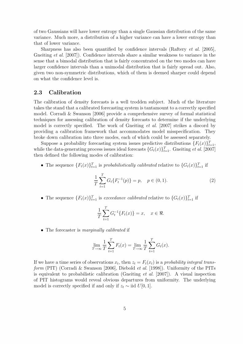
The first quality considered was sharpness. A sample of density forecasts from twoensemble forecasts at a forecast lead time of 6.4 ms is shown in figure 1. On the left aredensity forecasts resulting from estimation without the climatology and those on theright were obtained by mixing with the climatology. It is evident, by visual inspection,that including climatology resulted in predictive distributions that were sharper (nar-rower). Note that all the predictive distributions shown in figure 1 are clearly sharperthan the climatology, which is shown in figure 2.

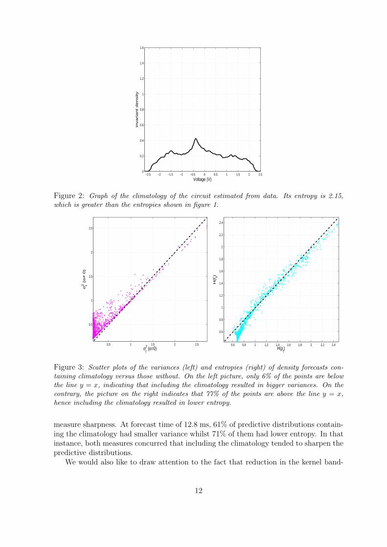
Sharpness was assessed further by computing the corresponding variances and den-sity entropies (see figures 3). The graph on the left shows a scatter plot of the variances

10

−2.5 −2 −1.5 −1 −0.5 0 0.5 1 1.5 2 2.50

0.2

0.4

0.6

0.8

1

1.2

1.4

1.6

Voltage (V)

Pre

dic

tive

De

nsity

Variance = 0.15168, Entropy = 0.68665

−2.5 −2 −1.5 −1 −0.5 0 0.5 1 1.5 2 2.50

0.2

0.4

0.6

0.8

1

1.2

1.4

1.6

Voltage (V)

Pre

dic

tive

De

nsity

Variance = 0.21657, Entropy = 0.46334

−2.5 −2 −1.5 −1 −0.5 0 0.5 1 1.5 2 2.50

0.2

0.4

0.6

0.8

1

1.2

1.4

1.6

Voltage (V)

Pre

dic

tive

De

nsity

Variance = 0.29744, Entropy = 1.1231

−2.5 −2 −1.5 −1 −0.5 0 0.5 1 1.5 2 2.50

0.2

0.4

0.6

0.8

1

1.2

1.4

1.6

Voltage (V)

Pre

dic

tive

De

nsity

Variance = 0.48003, Entropy = 1.0601

Figure 1: Graphs of density forecasts for the circuit at a forecast time of 6.4 ms. Figures onthe same row correspond to the same ensemble. The density forecasts on the left were obtainedby estimation without the climatology and those on the right were obtained by including theclimatology. Notice that including the climatology resulted in narrower distributions. Clearly,the lower entropies for the graphs on the right are a reflection of the noticeable increase insharpness.

of the predictive distributions containing the climatology against those without it. Only6% of the predictive distributions mixed with the climatology resulted in variance reduc-tion. Based on this graph, one could conclude that including the climatology resulted inpredictive distributions that were more spread out. We contend that it is better to useentropy to measure sharpness. On the scatter plot of density entropies on the right handside of figure 3, 77% of the points lie below the line y = x, implying that including theclimatology generally yielded sharper predictive distributions. This example illustratesthat one’s conclusions can vary depending on whether they use entropy or variance to

11

−2.5 −2 −1.5 −1 −0.5 0 0.5 1 1.5 2 2.50

0.2

0.4

0.6

0.8

1

1.2

1.4

1.6

Voltage (V)

inva

ria

nt

de

nsity

Figure 2: Graph of the climatology of the circuit estimated from data. Its entropy is 2.15,which is greater than the entropies shown in figure 1.

0.5 1 1.5 2 2.5

0.5

1

1.5

2

2.5

σt2 (

α≠

0)

σt2 (α=0)

0.6 0.8 1 1.2 1.4 1.6 1.8 2 2.2 2.4

0.6

0.8

1

1.2

1.4

1.6

1.8

2

2.2

2.4

H(f

t)

H(ρt)

Figure 3: Scatter plots of the variances (left) and entropies (right) of density forecasts con-taining climatology versus those without. On the left picture, only 6% of the points are belowthe line y = x, indicating that including the climatology resulted in bigger variances. On thecontrary, the picture on the right indicates that 77% of the points are above the line y = x,hence including the climatology resulted in lower entropy.

measure sharpness. At forecast time of 12.8 ms, 61% of predictive distributions contain-ing the climatology had smaller variance whilst 71% of them had lower entropy. In thatinstance, both measures concurred that including the climatology tended to sharpen thepredictive distributions.

We would also like to draw attention to the fact that reduction in the kernel band-

12

0 2 4 6 8 10 12 14 160

0.002

0.004

0.006

0.008

0.01

0.012

forecast time (ms)

He

llin

ge

r d

ista

nce

α=1α≠ 1

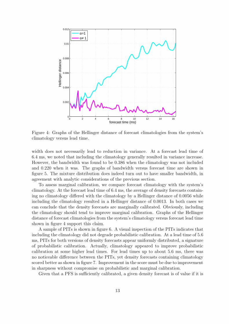
Figure 4: Graphs of the Hellinger distance of forecast climatologies from the system’sclimatology versus lead time.

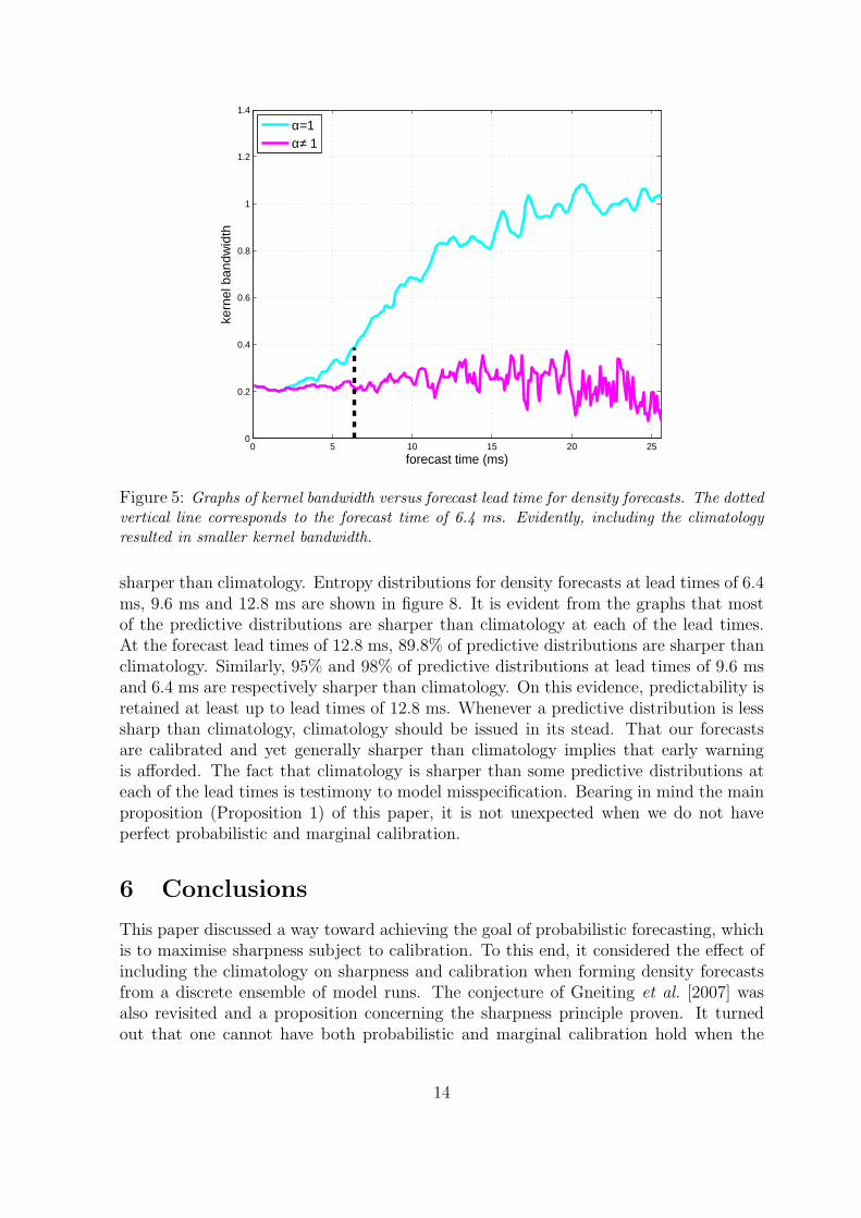
width does not necessarily lead to reduction in variance. At a forecast lead time of6.4 ms, we noted that including the climatology generally resulted in variance increase.However, the bandwidth was found to be 0.386 when the climatology was not includedand 0.220 when it was. The graphs of bandwidth versus forecast time are shown infigure 5. The mixture distribution does indeed turn out to have smaller bandwidth, inagreement with analytic considerations of the previous section.

To assess marginal calibration, we compare forecast climatology with the system’sclimatology. At the forecast lead time of 6.4 ms, the average of density forecasts contain-ing no climatology differed with the climatology by a Hellinger distance of 0.0056 whileincluding the climatology resulted in a Hellinger distance of 0.0013. In both cases wecan conclude that the density forecasts are marginally calibrated. Obviously, includingthe climatology should tend to improve marginal calibration. Graphs of the Hellingerdistance of forecast climatologies from the system’s climatology versus forecast lead timeshown in figure 4 support this claim.

A sample of PITs is shown in figure 6. A visual inspection of the PITs indicates thatincluding the climatology did not degrade probabilistic calibration. At a lead time of 5.6ms, PITs for both versions of density forecasts appear uniformly distributed, a signatureof probabilistic calibration. Actually, climatology appeared to improve probabilisticcalibration at some higher lead times. For lead times up to about 5.6 ms, there wasno noticeable difference between the PITs, yet density forecasts containing climatologyscored better as shown in figure 7. Improvement in the score must be due to improvementin sharpness without compromise on probabilistic and marginal calibration.

Given that a PFS is sufficiently calibrated, a given density forecast is of value if it is

13

0 5 10 15 20 250

0.2

0.4

0.6

0.8

1

1.2

1.4

forecast time (ms)

kern

el b

andw

idth

α=1α≠ 1

Figure 5: Graphs of kernel bandwidth versus forecast lead time for density forecasts. The dottedvertical line corresponds to the forecast time of 6.4 ms. Evidently, including the climatologyresulted in smaller kernel bandwidth.

sharper than climatology. Entropy distributions for density forecasts at lead times of 6.4ms, 9.6 ms and 12.8 ms are shown in figure 8. It is evident from the graphs that mostof the predictive distributions are sharper than climatology at each of the lead times.At the forecast lead times of 12.8 ms, 89.8% of predictive distributions are sharper thanclimatology. Similarly, 95% and 98% of predictive distributions at lead times of 9.6 msand 6.4 ms are respectively sharper than climatology. On this evidence, predictability isretained at least up to lead times of 12.8 ms. Whenever a predictive distribution is lesssharp than climatology, climatology should be issued in its stead. That our forecastsare calibrated and yet generally sharper than climatology implies that early warningis afforded. The fact that climatology is sharper than some predictive distributions ateach of the lead times is testimony to model misspecification. Bearing in mind the mainproposition (Proposition 1) of this paper, it is not unexpected when we do not haveperfect probabilistic and marginal calibration.

6 Conclusions

This paper discussed a way toward achieving the goal of probabilistic forecasting, whichis to maximise sharpness subject to calibration. To this end, it considered the effect ofincluding the climatology on sharpness and calibration when forming density forecastsfrom a discrete ensemble of model runs. The conjecture of Gneiting et al. [2007] wasalso revisited and a proposition concerning the sharpness principle proven. It turnedout that one cannot have both probabilistic and marginal calibration hold when the

14

0 0.1 0.2 0.3 0.4 0.5 0.6 0.7 0.8 0.9 10

10

20

30

40

50

60

70

80

90

100

110

PIT values

Fre

qu

en

cy

lead time, τ = 5.6

α=1α ≠ 1

,0 0.1 0.2 0.3 0.4 0.5 0.6 0.7 0.8 0.9 1

0

10

20

30

40

50

60

70

80

90

100

110

PIT values

Fre

qu

en

cy

lead time, τ = 6.4

α=1α ≠ 1

0 0.1 0.2 0.3 0.4 0.5 0.6 0.7 0.8 0.9 10

10

20

30

40

50

60

70

80

90

100

110

PIT values

Fre

qu

en

cy

lead time, τ = 9.6

α=1α ≠ 1

,0 0.1 0.2 0.3 0.4 0.5 0.6 0.7 0.8 0.9 1

0

10

20

30

40

50

60

70

80

90

100

110

PIT values

Fre

qu

en

cy

lead time, τ = 12.8

α=1α ≠ 1

Figure 6: Top: Graphs of probability integral transforms for predictive distributions at variouslead times. A visual inspection suggests that including climatology via the logarithmic scoringrule tends to improve probabilistic calibration.

15

5 10 15 20 25

−2

−1.5

−1

−0.5

0

0.5

forecast time (x10−3s)

⟨ IG

N ⟩

No climatologyWith climatology

,5 10 15 20 25

0.1

0.2

0.3

0.4

0.5

0.6

0.7

0.8

0.9

1

forecast time (x10−3s)

α (

mix

ture

we

igh

t)Figure 7: Left: Graphs of out-of-sample average Ignorance, with the associated 95% confidenceintervals, versus forecast time for density forecasts with and without the climatology. Theaverage Ignorance is given relative to the entropy of the climatology. Right: Graph of themixture weight versus forecast time. Notice from the left graph that if we do not includethe climatology, we lose predictability after about 13 ms. On the other hand, including theclimatology affords better performance up to 20 ms.

underlying model is misspecified unless they settle for the climatological forecaster. Inlight of this fact, it has been suggested that one should scale down their calibrationexpectations when facing model misspecification.

It was found that including the climatology via the logarithmic scoring rule tendedto improve marginal and probabilistic calibration. This was accompanied by a cor-responding increase in sharpness as measured by entropy. Improvement in marginalcalibration increased with lead time with no compromise to probabilistic calibration.It has also been argued that sharpness is better captured by entropy as opposed tovariance. Fairly calibrated predictive distributions at higher lead times were found tobe generally sharper than climatology, thus affording early warning. Crucially, though,some of the density forecasts may have larger entropy than the climatology. Such fore-casts have to be rejected in favour of the climatology, which is sharper. Even thoughthese observations were made on a nonlinear system, they may be useful in linear timeseries analysis as well, and/or when the model is stochastic. An open problem is todetermine analytically why including the climatology via the logarithmic scoring ruletends to maintain or improve probabilistic calibration.

Acknowledgements

The author would like to acknowledge useful discussions with members of the CATSgroup at LSE and the Applied Dynamical Systems and Inverse Problems group atOxford, and to thank David Allwright for his great insights especially pointing outProposition 4. This work was supported by the RCUK Digital Economy Programme.

16

0.4 0.6 0.8 1 1.2 1.4 1.6 1.8 2 2.2 2.40

20

40

60

80

100

120

140

density entropy

Freq

uenc

y

τ=6.4 msτ=9.6 msτ=12.8 ms

Figure 8: Entropy distributions for density forecasts containing climatology at three differentforecast lead times. The dash-dotted line corresponds to the entropy of the climatology. Densityforecasts whose entropies exceed that of climatology should be rejected in its favour.

References

Brier GW, 1950. Verification of forecasts expressed in terms of probability. MonthlyWeather Review 78:1–3.

Broecker J, 2009. Reliability, sufficiency, and the decomposition of proper scores. Quar-terly Journal of the Royal Meteorological Society 135:1512–1519.

Broecker J, Smith LA, 2008. From Ensemble Forecasting to Predictive DistributionFunctions. Tellus A 60:663.

Bross IDJ, 1953. Design for Decision: an introduction to statistical decision-making.New York: Macmillan.

Corradi V, Swanson NR, 2006. Predictive density evaluation, in Handbook of EconomicForecasting, volume 1. North-Holland.

Dawid AP, 1984. Present position and potential developments: Some Personal Views:Statistical Theory: The Prequencial Approach. J. R. Statist. Soc. A 147:278–292.

Diebold FX, Gunther TA, Tay AS, 1998. Evaluating density forecasts with applicationto financial risk management. International Economics Review 39:863–883.

Gneiting T, 2008. Probabilistic forecasting. J. R. Statist. Soc A 171:319–321.

Gneiting T, Balabdaoui F, Raftery AE, 2007. Probabilistic forecasts, calibration andsharpness. J. R. Statist. Soc. B 69:243–268.

17

Gneiting T, Raftery AE, 2007. Strictly proper scoring rules, prediction and estimation.J. Amer. Math. Soc. 102:359–378.

Good IJ, 1952. Rational decisions. Journal of the Royal Statistical Society. Series B(Methodological) 14:107–114.

Hall SG, Mitchell J, 2007. Combining density forecasts. International Journal of Fore-casting 23:1–13.

Hirschman II, 1957. A note on entropy. American Journal of Mathematics 79:152–156.

Kelly, 1956. A new interpretation of information rate. Bell Systems Technical Journal35:916–926.

Knorr-Held L, Rainer E, 2001. Projections of lung cancer in West Germany: A casestudy in bayesian prediction. Biostatistics 2:109–129.

Kullback S, Leibler RA, 1951. On Information and Sufficiency. The Annals of Mathe-matical Statistics 22:79–86.

Lawrence M, Goodwin P, Marcus O, Onkal D, 2006. Judgmental forecasting: A reviewof progress over the last 25 years. International Journal of Forecasting 22:493–518.

Murphy AH, 1993. What is a good forecast? An essay on the nature and goodness inweather forecasting. Weather and Forecasting 8:281–293.

Murphy AH, Wilks DS, 1998. A case study of the use of statistical models in the forecastverification: Precipitation probability forecasts. Weather and Forecasting 13:795–810.

Pal S, 2009. A note on a conjectured sharpness principle for probabilistic forecastingwith calibration. Biometrika 96:1019–1023.

Parzen E, 1962. On the Estimation of a Probability Density Function and Mode. TheAnnals of Mathematical Statistics 33:1065–1076.

Pollard D, 2002. A User’s Guide to Measure Theoretic Probability. Cambridge UniversityPress.

Raftery AE, Gneiting T, Balabdaoui F, Polakowski M, 2005. Using Bayesian ModelAveraging to Calibrate Forecast Ensembles. Monthly Weather Review 133:1155–1174.

Roulston MS, Smith LA, 2002. Evaluating Probabilistic Forecasts Using InformationTheory. Monthly Weather Review 130:1653–1660.

Saunders F, 1958. The evaluation of subjective probability forecasts. Cambridge, Mas-sachusetts Institute of Technology, Department of Meteorology, Contact AF 19(604)-1305, Sci. Rept. 5.

Shannon CE, 1948. A Mathematical theory of communication. Bell Systems TechnologyJournal 27:379–423,623–656.

18

Shannon CE, editor, 1949. Communication in the presence of noise, volume 37. Pro.Institute of Radio Engineers.

Silverman BW, 1986. Density Estimation for Statistics and Data Analysis. Chapmanand Hall, first edition.

White H, 1982. Maximum likelihood estimation of misspecified models. Econometrica50:1–25.

White H, 1994. Estimation, Inference and Specification Analysis. New York: CambridgeUniversity Press.

Wilks DS, 2006. Statistical Methods in the Atmospheric Sciences. Academic Press, 2nded edition.

A Generalised Construction of Probabilistically Cal-

ibrated Forecasts

PROPOSITION 4. Suppose that Gt is a continuous strictly increasing distributionfunction on an interval It. Let I be any interval and choose for each t a strictly increasingcontinuous map ht : I → It. A probabilistically calibrated forecast distribution functionprecisely takes the form1

Fs(xs) =1

T

T∑

t=1

Gt

[

ht

{

h−1s (xs)

}]

. (11)

Equation (11) is just Gneiting et al. [2007]’s construction in § 2.4 except that T isgeneral rather than 2 and the linear maps x and x/a that Gneiting et al. [2007] use arereplaced by the nonlinear maps ht. Note that each Fs is a strictly increasing continuousdistribution on Is and they are probabilistically calibrated forecasts of the Gt’s, becausegiven 0 < p < 1 there is some x in I with

p =1

T

T∑

t=1

Gt {ht(x)} = Fs {hs(x)} ,

whence F−1t (p) = ht(x) and

1

T

T∑

t=1

Gt

{

F−1t (p)

}

=1

T

T∑

t=1

Gt {ht(x)} = p.

Moreover, any probabilistically calibrated forecast of Gt takes exactly this form. Tosee this, let I be any interval and h1 be any suitable map from I onto I1 and then define

1This proposition and its proof were kindly worked out and privately communicated to me by

David Allwright who is at the Oxford Centre for Industrial and Applied Mathematics.

19

ht(x) = F−1t [F1{h1(x)}]. It then follows that

1

T

T∑

t=1

Gt

[

ht

{

h−1s (xs)

}]

=1

T

T∑

t=1

Gt

[

F−1t {Fs(xs)}

]

= Fs(xs).

The first equality follows by definition of the ht functions and the next by the proba-bilistic calibration property. Hence the Ft’s have exactly the form of the construction.

B Proof of Proposition 1

Using proposition 4, probabilistic calibration implies that Ft takes precisely the formgiven in (11). If the sequence {Ft} is also finite marginally calibrated, we can substi-tute (11) into (3) to obtain

1

T (T − 1)

T∑

t=1

T∑

s=1,s 6=t

Gt

[

ht

{

h−1s (x)

}]

=1

T

T∑

t=1

Gt(x), T ≥ 2.

It is, therefore, required that Gt [ht {h−1s (x)}] = Gi(x), where i ∈ {1, .., T}. If Gt[ht{h−1

s (x)}] =Gs(x) for any s, then the forecasts {Ft} are ideal. On the other hand, if Gt[ht{h−1

s (x)}] =Gt(x), then we have the finite climatological forecaster.

We now wish to show that a non-climatological forecaster who is both probabilis-tically and marginally calibrated is precisely the ideal forecaster. Consider Fs(x) asdefined by equation (11) for a given s. Suppose there exists q such that

Gt[ht{h−1s (x)}] = Gs(x), for all t ≤ q (12)

andGt[ht{h−1

s (x)] = Gt(x) for all t > q. (13)

Equation (12) implies that Gs[hs{h−1t (x)}] = Gt(x) for all t ≤ q while (13) implies that

ht(x) = hs(x) for all t > q. Fs(x) contains q counts of Gs(x). Each

Fi(x) =1

T

T∑

t=1

Gt

[

ht

{

h−1i (x)

}]

,

i 6= s, contains 0 counts of Gs(x) if i ≤ q. If i > q, we get

Gt[ht{h−1i (x)}] = Gt[ht{h−1

s (x)}] = Gs(x),

for all t ≤ q. The first equality follows from noting that hi(x) = hs(x) and the secondfrom applying (12). Hence each Fi(x) contains q counts of Gs(x). Therefore, all thesummations on the right hand side of the forecasters contain q + (T − q)q counts ofGs(x). Finite marginal calibration imposes the requirement that q + (T − q)q = T ,which holds if and only if q = T . But q = T implies that we have ideal forecasts.

More generally, the sequence {Gt[ht{h−1s (x)}]}t>q may contain multiplicities of the

Gt(x) terms. This means that, for a given t = r > q for which Gr[hr{h−1s (x)}] = Gr(x),

20

there may be at least another p 6= r and p > q such that Gp[hp{h−1s (x)}] = Gr(x). Let

j be the number of all p’s for all r’s as defined above. Then the total number of Gs(x)terms over the right hand sides of all Fi(x) and Fs(x) is q + (T − q − j)q. Marginalcalibration imposes the condition that

q + (T − q − j)q = T ⇒ q2 − q(T − j + 1) + T = 0.

For the above quadratic equation to have an integer solution in q, the discriminant mustbe a perfect square, which happens if and only if j = 0. Hence a non-climatologicalforecaster who is both finite marginally and probabilistically calibrated must have issuedideal forecasts.

C Proofs of Propositions 2 and 3

Proof of proposition 2: The second partial derivative of equation (8) with respect tothe mixture parameter α yields

∂2〈IGN〉∂α2

=1

T

T∑

t=1

{

ρ(t)(st|VT ) − ρc(st)

f (t)(st|VT )

}2

.

Hence the first derivative of 〈IGN〉 with respect to α is an increasing function of α. Itfollows that the first derivative will have a zero at some α = α∗ ∈ (0, 1) if and only if

∂〈IGN〉∂α

∣

∣

∣

∣

α=0

< 0 and∂〈IGN〉

∂α

∣

∣

∣

∣

α=1

> 0.

These are essentially the inequalities in the proposition. The second derivative impliesthat α∗ is a global minimiser of the score.

Proof of proposition 3: ∂〈IGN〉/∂σ = 0 implies that

σ2∗

1

T

T∑

t=1

ρ(t)(st|VT )

f (t)(st|VT )=

1

T

T∑

t=1

{

st − X(t)1

}2 ρ(t)(st|VT )

f (t)(st|VT ).

But ∂〈IGN〉/∂α = 0 implies that

1

T

T∑

t=1

ρ(t)(st|VT )

f (t)(st|VT )= 1,

which may be plugged into the left hand side of the previous equation to complete theproof.

21