NBER WORKING PAPER SERIES

EARLY LIFE ENVIRONMENT AND RACIAL INEQUALITY IN EDUCATIONAND EARNINGS IN THE UNITED STATES

Kenneth Y. ChayJonathan Guryan

Bhashkar Mazumder

Working Paper 20539http://www.nber.org/papers/w20539

NATIONAL BUREAU OF ECONOMIC RESEARCH1050 Massachusetts Avenue

Cambridge, MA 02138October 2014

We thank numerous seminar participants and Blaise Melly for helpful comments. The views expressedhere do not reflect the views of the Federal Reserve system. All errors are our own. The views expressedherein are those of the authors and do not necessarily reflect the views of the National Bureau of EconomicResearch.

NBER working papers are circulated for discussion and comment purposes. They have not been peer-reviewed or been subject to the review by the NBER Board of Directors that accompanies officialNBER publications.

© 2014 by Kenneth Y. Chay, Jonathan Guryan, and Bhashkar Mazumder. All rights reserved. Shortsections of text, not to exceed two paragraphs, may be quoted without explicit permission providedthat full credit, including © notice, is given to the source.

Early Life Environment and Racial Inequality in Education and Earnings in the United StatesKenneth Y. Chay, Jonathan Guryan, and Bhashkar MazumderNBER Working Paper No. 20539October 2014JEL No. I12,I14,J13,J24,J31

ABSTRACT

Chay, Guryan and Mazumder (2009) found substantial racial convergence in AFQT and NAEP scoresacross cohorts born in the 1960’s and early 1970’s that was concentrated among blacks in the South.We demonstrated a close tracking between variation in the test score convergence across states andracial convergence in measures of health and hospital access in the years immediately after birth.This study analyzes whether the across-cohort patterns in the black-white education and earnings gapsmatch those in early life health and test scores already established. It also addresses caveats in theearlier study, such as unobserved selection into taking the AFQT and potential discrepancies betweenstate-of-birth and state-of-test taking.

With Census data, we find: i) a significant narrowing across the same cohorts in education gaps drivenprimarily by a relative increase in the probability of blacks going to college; and ii) a similar convergencein relative earnings that is insensitive to adjustments for employment selection, as well as time andage effects that vary by race and state-of-residence. The variation in racial convergence across birthstates matches the patterns in the earlier study. The magnitude of the earnings gains is greater thancan be explained by only the black gains in education and test scores for reasonable estimates of thereturns to human capital. This suggests that other pre-market, productivity factors also improved acrosssuccessive cohorts of blacks born in the South between the early 1960’s and early 1970’s. Finally,our cohort-based hypothesis provides a cohesive explanation for the aggregate patterns in several,previously disconnected literatures.

Kenneth Y. ChayDepartment of EconomicsBrown UniversityBox BProvidence, RI 02912and NBERKenneth_Chay@brown.edu

Jonathan GuryanNorthwestern UniversityInstitute for Policy Research2040 Sheridan RoadEvanston, IL 60208and NBERj-guryan@northwestern.edu

Bhashkar MazumderFederal Reserve Bank of Chicago230 S. LaSalle StreetChicago, IL 60604bhash.mazumder@gmail.com

1

I. Introduction

There has been a growing focus on the importance of early life health and environment for long-

term well-being, such as adult health and human capital. Chay, Guryan and Mazumder (2009) used two

data sources – the Long Term Trends NAEP and AFQT scores for the universe of applicants to the U.S.

military – to show: 1) the black-white convergence in test scores during the 1980s’ was due to relative

improvements across successive cohorts of blacks born between 1963 and the early 1970’s; and 2) these

across-cohort gains were concentrated among blacks in the South. We found that the timing and variation

across states in the AFQT convergence closely tracks racial convergence in measures of health and

hospital access in the years soon after birth; and found that they are highly correlated with post-neonatal

mortality rates (and not with neonatal mortality and low birth weight rates). As the competing hypotheses

did not exhibit similar patterns, we concluded that health investments through increased access during the

first three years of life – due to the racial integration of Southern hospitals in the 1960’s, for example –

led to gains in cognitive skills among Southern-born blacks measurable at ages 17 and 18.

Here, we analyze whether the across-cohort patterns in racial gaps in education and earnings

match those established in the previous paper. If correct, our hypothesis would suggest similar patterns in

other measures of human capital and economic productivity. Further, this study can address two of the

primary caveats in our previous analysis. First, while the size and scope of the AFQT data allowed us to

construct narrow comparisons across birth cohorts and states, the test takers are not representative of the

U.S. population. Although our analyses used several approaches to correct for this nonrandomness,

selection on unobservables could remain as a source of bias. Second, the data provided the state in which

the test was taken but not the actual state-of-birth. Thus, the results could be biased by systematic

discrepancies between state-of-birth and state-of-test taking – e.g., due to nonrandom migration between

birth and age 17 – that vary by race, state, age and time.

Using data from the 1990 and 2000 U.S. Censuses and the 2005 to 2008 American Community

Surveys, we study the changes across cohorts in educational attainment, annual earnings and the

incidence of work disability for blacks and whites born between the mid-1950’s and mid-1970’s. As

these data include the state-of-birth of respondents and are representative of the U.S. population, they

directly address whether the relations between early-life health and later-life skills shown in Chay,

Guryan and Mazumder (2009) are biased by nonrandom migration or selection into test taking.

2

The analysis compares black-white gaps by birth year and region (or state) of birth, while

adjusting for race-specific time and age effects. In contrast to Chay, Guryan and Mazumder (2009), we

can also control for state-of-residence (interacted with race, age and time) effects, which results in

comparisons of blacks (and whites) who live in the same state but were born in different regions or states.

As the relative gains in early-life health were much greater for blacks born in Southern than in non-

Southern states, much of the analysis contrasts adult outcomes for blacks born in the South to their

counterparts born outside of the South; for example, in the states of the Rustbelt.

We find that the black-white education gap exhibits patterns by birth year and birth place that are

quite similar to those in cognitive scores. For example, the black white-gap in college-going is roughly

five percentage points greater for Southern-born men born in the 1950’s and early 1960’s than for their

Rustbelt-born counterparts, and this gap is stable across these birth years. For the later cohorts, however,

there is a striking narrowing of the college gap that continues until the early 1970’s cohorts, for whom

Southern-born black men are marginally more likely to go to college than their Rustbelt-born

counterparts. The results imply that the racial gaps in the completed education and college attendance of

Southern-born men were, respectively, 31 and 40 percent lower in the early 1970’s cohorts than in the

early 1960’s cohorts. We find similar patterns for women. Separate results from the October

supplements of the Current Population Survey show that these findings are driven by relative increases in

high school completion and college enrollment among Southern blacks as of ages 18 and 19.

Turning to annual earnings, we again find no convergence in the black-white gap of Southern-

born men relative to those born outside of the South for the 1950’s and early 1960’s birth cohorts. For the

cohorts born between 1963 and the early 1970’s, the black-white earnings gap falls by 0.07 to 0.08 log

points more among the Southern-born, and these results are insensitive to controls for race-by-year and

race-by-age effects interacted with state-of-residence. Thus, the finding holds even when comparing men

living in the same state who: i) were born in the same year but in different states; and ii) were born in the

same state but in different years. These specifications are quite unrestrictive with respect to labor market

conditions that vary by race, age and state.

The earnings convergence is driven mostly by cross-cohort gains for Southern-born blacks – that

is, white men exhibit very similar cross-cohort changes regardless of where they are born, and the same is

true of blacks born outside of the South and for blacks and whites born outside of the United States. The

3

earnings results are insensitive to different approaches to addressing selection into employment. As in

Chay, Guryan, and Mazumder (2009) we find that the variation in the cross-cohort racial convergence in

education and earnings by state-of-birth is strongly associated with measures of early life health and that

these associations hold even within region-of-birth. For example, racial gaps in post-neonatal mortality

rates in the years when the cohorts were born explain two-thirds and one-half of the variation in the cross-

cohort convergence in college-going and log-earnings, respectively.

The magnitude of the earnings convergence appears too large to be explained by only the black

gains in education and test scores. Roughly three-quarters of the relative earnings convergence remains

after adjusting for the convergence in completed education, and the AFQT gains documented in the

earlier study cannot explain this remainder even under unrealistic assumptions on the independence of

education and test score gains. Further, the between-cohort earnings gains for Southern-born blacks have

a significant interaction with completed education – for example, there is a 0.11 log-point convergence

for black college graduates and a 0.02 convergence among the high school educated. This suggests

unobserved complementarity in human capital formation and/or improvements in other pre-market,

productivity factors for blacks born in the South between the early 1960’s and early 1970’s. Consistent

with this, we find that black disability rates also fell between the two sets of Southern birth cohorts

relative to blacks born outside of the South.

We conclude that our cohort-based hypothesis provides a cohesive explanation for the stylized

facts in previously disconnected literatures that required several, different hypotheses. Prior studies have

documented black gains in test scores in the early 1980s (Jenks and Phillips 1998, Cook and Evans 2000,

Dickens and Flynn 2006, Neal 2006, Magnuson and Waldfogel 2008), in college enrollment in the mid-

1980s (Hauser 1993, Kane 1994), and in relative earnings throughout the 1990s (Couch and Daly 2002,

Card and DiNardo 2002, Western and Pettit 2005). We demonstrate that nearly all of these gains were

concentrated among blacks born in the South between roughly 1963 and 1971; and, therefore, not

primarily the result of contemporary causes in the 1980s and 1990s. The results indicate, for example,

that the black earnings gains in the 1990s were the results of human capital improvements triggered by

events 25 to 30 years earlier – that is, the Civil Rights and War on Poverty periods.

4

II. Data and Estimation

Chay, Guryan and Mazumder (2009) found substantial racial convergence in cognitive test scores

across cohorts born in the 1960’s and early 1970’s. These gains were concentrated among blacks in the

South and strongly associated with state-specific, racial convergence in measures of early life health and

hospital access. Two caveats arose in the analysis, however. Both sources of testing data provided the

state in which the test was administered but not the state-of-birth of the individual; and the AFQT data

came from the universe of applicants to the U.S. military and therefore are not representative of all 17 and

18 year-old men in the cohorts of interest.

The Census data used in this study directly addresses both of these issues. They also allow us to

examine whether similar patterns exist in other measures of human capital and economic productivity,

such as completed education and annual earnings. Further, this study can examine the educational

attainment and earnings of black women, who also should have been affected by changes in early life

environment. While our earlier work examined girls’ test scores in the NAEP, we did not do this in the

AFQT data due to the much greater selectivity issues.

It is critical in this study to plausibly distinguish between time, age and birth year effects;

something that cannot be done without identifying assumptions due to the perfect collinearity of these

effects. In typical survey designs, the year-of-birth is equal to the survey year minus an individual’s age

(in years) at the time of the survey. While not “solving” this identification problem, one advantage of the

AFQT data used in Chay, Guryan and Mazumder (2009) is that the test was administered on a rolling

basis throughout a calendar year. In this case, survey year, age-in-years and birth year are not perfectly

collinear since, for example, there can be 17-year-olds born in the same year who happen to take the exam

in different calendar years. Of course, completely unrestricted effects at a fine enough level of detail –

exact birthday, exact age at and date of exam (or survey) – are collinear.

A. Data

We combine six-percent samples from each of the 1990 and 2000 Censuses with one-percent

samples from each American Community Survey (ACS) in 2005 to 2008.1 The income questions in the

1 The extracts are from the IPUMS USA website maintained by the Minnesota Population Center. For 1990 we combined the five-percent State sample and the one-percent Metropolitan sample. For 2000 we combined the five-percent sample and the one-percent sample. The ACS data are one-percent samples. We do not use the data from

5

Censuses refer to the previous calendar year, while similar questions in the ACS refer to the past twelve

months up to the time of filling out the questionnaire. Since individuals are surveyed throughout the year,

the income measures in the ACS are a mix of the current and previous year.2

Our sample contains individuals aged 26 to 45 who were born between 1945 and 1982. Much of

the analysis focuses on cohorts born between 1951 and 1977. We further restrict the sample to non-

Hispanic whites and blacks and drop individuals with either missing or imputed data on gender, race,

Hispanic ethnicity, year-of-birth, state-of-birth or state-of-residence. We further drop observations with

missing or imputed data on completed education and annual wage and salary income when examining

those outcomes.

For education, we analyze two outcomes of interest – years of completed education and

likelihood of attending college. For annual earnings, we use the individual’s total, pre-tax wage and

salary income for the year prior to the survey. We convert the earnings data into 2007 dollars using the

CPI-U and use its natural logarithm as the outcome of interest. We present separate earnings results for

men who are full-time, full-year workers, which we define as those who worked at least 20 hours-per-

week and at least 26 weeks of the year. We also examine full-time, full-year employment as an outcome.

Finally, we examine disability incidence, which we discuss in more detail below.

Importantly, the Census and ACS data provide the state-of-birth of respondents. Our analysis

often contrasts groups by the region-of-birth based on the state-of-birth. The “South” consists of

Alabama, Arkansas, Florida, Georgia, Louisiana, Mississippi, North Carolina, South Carolina, Tennessee

and Virginia; the “Rustbelt” consists of Illinois, Indiana, Michigan, Missouri, New York, Ohio and

Pennsylvania; the “Border” states include Delaware, Kentucky, Maryland, Texas and West Virginia; and

the “Other” region contains the remaining twenty-eight U.S. states and the District of Columbia. We also

analyze non-Hispanic whites and blacks who were born outside of the United States.

Table 1 presents summary information on our samples of 4.7 million men and 4.9 million women,

who are aged 26 to 45 and born between 1945 and 1982. In the male sample [columns (1a) to (1d)]: black

representation is highest among men born in the South (27.4%); the education data contain few missing

the demonstration phase of the ACS (2001 to 2004) because they were only roughly 1-in-240 samples and covered only 37 percent of the geography of the U.S. (US Census Bureau, 2006) 2 Employment rates for men (especially for the less-educated) fell precipitously in the 2nd-half of 2008 through most of 2009. As a result, we do not add the 2009 ACS to our analysis sample due to the impact of the “Great Recession” on selection into the annual earnings sample.

6

observations; educational attainment is lowest among Southern-born men, both black and white; missing

data are a bigger issue in the earnings sample, particularly when utilizing the natural logarithm of

earnings; the black-white annual earnings gaps are large in each region-of-birth, with earnings ratios

roughly equal to 0.6; the earnings gaps are smaller among full-time, full-year workers (earnings ratios

above 0.7); annual earnings are lowest among Southern-born men, both black and white; and blacks have

lower full-time, full-year worker rates and higher missing data rates for ln-earnings, though the disparities

are similar by region-of-birth.

The patterns for women [columns (2a) to (2d)] are similar, with the following exceptions:

women, especially black women, are better-educated than their male counterparts; the racial gap in

education is smaller for women than for men; women also have small racial gaps in annual earnings –

e.g., black women born in the “Other” states earn slightly more, on average, than white women – but the

gaps are slightly larger among full-time, full-year workers; black and white women have similar rates of

being full-time, full-year workers and of having missing data on ln-earnings. White women are much less

likely to be full-time, full-year workers than white men, while these rates are more similar among blacks.

Below, we focus primarily on the results for men but also present and discuss the findings for women.

The conclusions are similar for both genders.

B. Econometric Models

We now discuss our models for distinguishing birth cohort effects in racial gaps in education and

earnings from age and time effects. The figures below present birth cohort effects by race and place-of-

birth, which are estimated from regression models of the form:

(1) ( ) icatpobwb

cpobw

cicat porracetimeagefy εθλ +++= − ,,,,,

where i indexes individuals, c indexes year of birth, a indexes age in the survey year, and t indexes the

survey year. The outcome variable, y, is completed education or annual earnings; pob and por index

place-of-birth and place-of-residence, respectively; and ε is an error term. The regressions are weighed

by the individual sampling weights.

The parameters of interest, pobwbc

,−θ , measure the black-white gaps by birth year and birthplace;

while the parameters, pobwc

,λ , are the birth cohort effect for whites by birthplace. Given the findings in

Chay, Guryan and Mazumder (2009), we focus on contrasting the black-white cohort effects for those

7

born in the South to those born in the Rustbelt states – e.g., ( )rbeltwbc

southwbc

,, −− −θθ . To confirm that the

patterns are driven by Southern-born blacks, we also contrast: i) the racial gaps for blacks born in areas

outside of the South and Rustbelt (including the foreign-born) to those born in the Rustbelt; and ii) the

cohort effects for whites born in each area relative to those born in the Rustbelt.

By using the Rustbelt-born as the baseline for comparison, our regressions can include

unrestricted race-by-age and race-by-time effects and still identify the birth cohort effects relative to those

born in the Rustbelt (the levels of the Rustbelt cohort effects will not be identified). In this case, the

implicit assumption identifying the relative cohort effects is that the race-specific age and time effects do

not vary by birthplace. Indeed, we can still identify the relative cohort effects even when including race-

specific age and time effects that vary by place-of-residence, as there are many blacks and whites who, by

the ages of 26 to 45, live and work in a different state/region than the one they were born in. In this case,

the analysis is quite unrestricted with respect to race-specific age and time effects in the prevailing local

labor market. It implicitly assumes, however, that blacks (and whites) of the same age, who live in the

same place in the same year as adults but were born in different places, are only distinguished by their

birthplace and not by other unobserved factors.

The figures below present the estimated, relative birth cohort effects from a few specifications of

the control function for race-specific age, time and place-of-residence effects; f(age, time, race, por) in

equation (1). To gauge the magnitudes and statistical significance of the relative racial convergence

across birth cohorts, we estimate the following regression model:

(2) ( ) ( ) ( )

( ) ( ) icatpobr

cpobwb

post

pobwbpre

pobwpost

pobwpreicat

porracetimeagefc

cccy

εγθ

θλλ

+++−=⋅

+−=⋅+−=⋅+−=⋅=−

−

,,,7219701

621960172197016219601),(,

,,,

where 1(∙) is an indicator function equal to one if the individual is born between 1960 and 1962 (or 1970

and 1972); (r) indexes race, and pobrc

),(γ are race-specific birth cohort effects, by place-of-birth, for those

individuals not born in either 1960-62 or 1970-72.3

Equation (2) fits early 1960’s and early 1970’s cohort averages to the figures generated by equation (1). One parameter of interest is ( ) ( )( )rbeltwb

prerbeltwb

postsouthwb

presouthwb

post,,,, −−−− −−− θθθθ – that is, the

difference-in-differences-in-differences (DDD) estimates of the between-cohort racial convergence for

3 As the survey data are for 1990, 2000, and 2005 to 2008 – and the samples are restricted to those aged 26 to 45 – individuals born between 1960 and 1962 are observed at the ages of 28 to 45, and individuals born between 1970 and 1972 are observed at ages 28 to 38.

8

the Southern-born relative to the Rustbelt-born. In the tables below, we also present the DDD estimates

for those born outside of the South and Rustbelt, and the DD estimates for whites – for example, ( ) ( )( )rbeltw

prerbeltw

postsouthw

presouthw

post,,,, λλλλ −−− .

We examine the sensitivity of the DDD (and DD) estimates to progressively more unrestricted

specifications of the race-specific age, time, and place-of-residence effects – f(age, time, race, por). For

completed education, our most unrestricted control function includes unrestricted race-age-year effects

and state-of-residence effects separately interacted with race, age and year effects. For annual earnings,

we utilize several different, flexible specifications that control for unrestricted race-age-year effects;

including one that also contains unrestricted state-of-residence-by-race-by-year effects and state-of-

residence-by-age effects, and another that contains unrestricted state-of-residence-by-race-by-age effects

and state-of-residence-by-year effects.

Before proceeding, we provide a concrete example of the comparisons made when the analysis

controls for state-of-residence effects in addition to race-age-time effects. Imagine four groups of blacks

and whites living in New York state in 2000, those: i) aged 30 and born in the South; ii) aged 30 and born

in the Rustbelt; iii) aged 38, born in the South; and iv) aged 38, born in the Rustbelt. The first two groups

were born in 1970, and the latter two groups in 1962. Our more flexible specifications estimate the

between-cohort racial convergence in the log-earnings of the Southern-born relative to the Rustbelt-born

by comparing the black-white gaps in the four groups of New Yorkers in 2000; ((i − ii) − (iii − iv)).

This comparison clearly controls for unrestricted race-by-age effects prevailing in the New York

labor market in 2000. It will provide a misleading conclusion on the impact of birth year on the relative

racial gaps of the Southern-born if the factors that led to living in New York as an adult in 2000 differed

between 30 and 38 year-old Southern-born blacks relative to Southern-born whites and relative to their

Rustbelt-born black and white counterparts. While such possibilities exist – e.g., nonrandom migration

by birthplace that coincides with these birth cohorts in a race-specific way – they are somewhat

complicated. Regardless, below we find that the estimated earnings gains across cohorts of Southern-

born blacks are insensitive to controlling for the state-of-residence effects, and are significant both for

men who reside in their state-of-birth and men who do not.

9

C. Selection Issues

The Census/ACS data used in this study are representative of the U.S. population; something that

is not true of the AFQT data analyzed in our earlier work. Thus, sample selection issues are significantly

reduced in this study. In the context of completed education, for example, our sample is only missing

individuals in the birth cohorts of interest who were institutionalized between the ages of 26 and 45 in the

survey years. When we analyzed institutionalization incidence, we found that restricting the sample to

the non-institutionalized leads, if anything, to a small downward bias in the estimated cross-cohort gains

for Southern-born blacks (see the Appendix for details).4

The sample selection issues are greater in the annual earnings analysis since it is based on those

with non-missing (and non-imputed) wage and salary income. These issues increase when the analysis is

further restricted to men who are “full-time, full-year” workers. We examine the sensitivity of our log-

earnings findings to several, different approaches to handling men with non-positive earnings. With

respect to earnings among full-time, full year workers, we apply equations (1) and (2) to the probability of

being employed at least 20 hours-per-week and at least 26 weeks of the year. We also apply these

equations to an indicator for having positive (non-missing, non-imputed) annual earnings.

In both cases, we find no evidence of differential selection probabilities across birth cohorts by

region-of-birth. As long as the potential sample selection bias can be summarized by a single-index –

e.g., there is a monotonic relationship between the probability of selection and annual earnings – then this

implies no selection bias in the across-cohort comparisons of the Southern- and Rustbelt-born.5 In this

case, the comparisons provide the average relative convergence across birth cohorts for the full-time, full-

year employed (but not for the population of men as a whole); sometimes referred to as the selected

average treatment effect (SATE).

4 The biggest issue vis-à-vis institutionalization is probably the significant increase in incarceration rates beginning in the 1980s, particularly of black men (Pettit and Western 2004). This would be problematic if the growth in incarceration rates between the early 1960’s and early 1970’s birth cohorts was greater for blacks born in the South than for those born in the Rustbelt. We find evidence that the reverse is true (see Appendix). 5 In the absence of plausible (and powerful) instruments for selection into work, one can construct bounds for the earnings effects in the presence of selection on unobservables. If the selection bias satisfies the “single-index” property (e.g., due to monotoncity), then the probability of selection is a sufficient statistic for the selection bias with no further restrictions placed on the outcome equation other than separability of the error term and regression function (Ahn and Powell 1993). Further, if the probability of selection is the same between comparison groups, then the bounds on the earnings effects collapse to a point (Lee 2009). While single-index sufficiency rules out worst case scenarios for selection (Manski 1990; Horowitz and Manski 2000), monotonicity seems a reasonable approximation in our context – i.e., as the latent probability of employment increases, latent earnings also increase.

10

We also estimate equations (1) and (2) using quantile regressions at the 25th, 50th and 75th

percentiles for the sample of all workers and the sample of full-time, full-year employed. When median

regressions are applied to the sample of all men with non-missing earnings, for example, the resulting

comparisons provide the median effect for the population of all workers. We also estimate quantile

regressions in which men with missing data are assigned annual earnings of one dollar (log-earnings

equal to zero) – that is, the lowest earnings possible. Since quantiles are order statistics, the resulting

estimator effectively treats these data as being below the conditional quantile of interest but puts no

weight on the distance of the observation from the conditional quantile. As long as the (conditional)

percentage of men with missing data is less than the quantile of interest, then the resulting comparisons

provide the population quantile effect for all men. Below, we find similar estimates of the parameters of

interest regardless of the approach and sample used.

III. Education Results

Figure 1 presents the differences between Southern- and Rustbelt-born men in their racial gaps in

educational attainment by birth year – that is, estimates of ( )rbeltwbc

southwbc

,, −− −θθ from equation (1). The

plots for completed years of education (Panel A) and for the incidence of attending college (Panel B)

come from a specification with no control variables and one with unrestricted race-by-age and state-of-

residence fixed effects. While results are only shown for the 1951 to 1977 birth cohorts, the estimation

sample includes men born between 1945 and 1982 in any of the regions of interest (South, Rustbelt,

Border, Other and Foreign).6

In Panel A, the racial gap in the completed schooling of Southern-born men relative to the

Rustbelt-born is stable through the late 1950s and early 1960s birth cohorts. While the racial gap for

these cohorts is slightly smaller among the Southern-born, Southern-born black men actually have less

education than their Rustbelt-born counterparts – in the 1960 cohort, Southern- and Rustbelt-born black

men have, on average, 12.5 and 13.0 years of completed education, respectively.7 Between the 1964 and

early 1970s cohorts, the racial gap for the Southern-born abruptly falls by 0.2 years relative to the

Rustbelt-born – in the 1972 cohort, Southern- and Rustbelt-born black men have 12.9 and 13.1 years of

6 For men born in 1951, we observe their educational attainment at ages 38 or 39 in the 1990 Census. For those born in 1977, educational attainment is observed at ages 28 to 31 in the 2005 to 2008 ACS. 7 In the 1960 cohort, Southern- and Rustbelt-born white men have 13.2 and 13.8 years of education, respectively.

11

education, on average. These patterns are unaltered when state-of-residence and interactions of race with

age are controlled for.8

Panel B shows that the education gains for black men born in the South in the mid-1960s and

early 1970s was primarily due to increased college attendance.9 For men born between 1951 and 1963,

the racial gap in the probability of attaining at least some college is 4-6 percentage points greater for the

Southern-born than for the Rustbelt-born. Strikingly, the relative disadvantage for Southern-born black

men is eliminated by the 1965 to 1968 birth cohorts, and by the early 1970s cohorts the racial gap is

smaller for the Southern-born than for the Rustbelt-born. In the 1960 cohort, the college incidence is 36.1

and 48.2 percent for black men born in the South and Rustbelt, respectively; while in the 1972 cohort, the

corresponding figures are 42.2 and 49.1 percent. The patterns are unaffected by adjustment for race-by-

age and state-of-residence fixed effects.

This relative improvement across birth cohorts in completed schooling, however, was not

experienced by black men born in states outside of the South or Border regions. Figure 2 presents the

(unadjusted) differences in educational attainment for men born in the South and in the “Other” region

relative to the Rustbelt-born. Panel A contains the between-region differences in the black-white gap,

while Panel B contains the between-region differences in the white level.

Panel A shows that, relative to the Rustbelt-born, the racial gaps in education for the Southern-

born and Other-born are quite similar to each other for the 1955 to 1963 cohorts. For cohorts born after

1963, the relative gaps among the Southern- and Other-born diverge markedly, with only the Southern-

born blacks experiencing a relative improvement. Thus, black men born in the South after the mid-1960s

also increased their educational attainment relative to blacks born in the Other region. Panel B shows

that, relative to Rustbelt-born whites, the average education levels for Southern- and Other-born white

men fluctuate relatively little between the 1955 and 1977 cohorts. Thus, the decline in the education gap

8 Men from all places of birth contribute to the state-of-residence and race-by-age effects. 9 There are some differences across the 1990 and 2000 Censuses and 2005 to 2008 ACS in how the completed schooling variable is recorded. We created a years of completed education variable that harmonizes these small differences, which is particularly straightforward for those with less than a high school degree. For those with more education: high school graduates and those with a GED are assigned 12 years of completed education; those with “some college, no degree” or with Associate degrees (program unspecified, occupational program, and academic program) are assigned 14 years of education; those with Bachelor’s, Master’s, Professional and Doctorate degrees are assigned 16, 18, 19 and 20 years of education, respectively.

12

among the later cohorts born in the South is driven entirely by gains made by black men, as there are no

relative changes for blacks born elsewhere or whites born in any region of the United States.

Figure 3 presents the analogous patterns for college-going rates, and their implications are the

same as those in Figure 2. Panels A and B demonstrate that the across-cohort improvement in college

attendance occurred exclusively among black men born in the South. In Panel A, the gaps for black men

born in the Rustbelt and Other states are similar to each other and are relatively stable across all of the

birth cohorts. For the Southern-born, the college attendance gap is 4 to 6 percentage points in the 1951 to

1963 cohorts, but converges sharply toward the gaps of the Rustbelt- and Other-born in the later cohorts.

Panel B shows that, relative to the Rustbelt-born, Southern-born white men are 6 to 9 percentage points

less likely to attend college, and Other-born whites are three percentage points more likely to get at least

some college education. These differences, though, fluctuate very little across the years of birth.

Tables 2 and 3 present the results from fitting equation (2) to the data underlying Figures 2 and 3,

respectively. Recall that equation (2) provides estimates of outcome differences between the 1960-1962

and 1970-1972 birth cohorts, by race and place-of-birth.10 The first column of each table contains the

unadjusted results, and the subsequent columns correspond with regressions that control for progressively

more fixed effects; with the final specification adjusting for unrestricted race-by-year-by-age effects and

state-of-residence separately interacted with race, year and age. Panel A of each table contains the cross-

cohort change in the racial gaps of men born in the South (or in the “Other” states or outside of the U.S.)

relative to those born in the Rustbelt – i.e., the DDD estimates of the difference between regions-of-birth

in the racial convergence across birth cohorts. Panel B contains the cross-cohort change in white levels

relative to the Rustbelt-born (the DD estimates).

Table 2 shows that relative to the Rustbelt-born, the black-white gap in education is 0.20 to 0.22

years smaller for those born in the South in 1970 to 1972 than for their counterparts born between 1960

and 1962. The cross-cohort racial convergence for the Southern-born is highly significant and increases

slightly, in both magnitude and statistical significance, as the regressions control for the state-of-residence

fixed effects and their interactions. These results match the patterns in Figure 1A and imply that the

10 When estimating equation (2), we restrict the sample to those born between 1955 and 1974. Individuals born in the “Border” states are included in the sample. While results for the Border-born are not presented in the tables, they are shown in some of the figures below.

13

racial gap in completed schooling for Southern-born men fell by 31 percent between the early 1960s and

early 1970s birth cohorts.11

Importantly, Table 2 also shows that Southern-born black men are the only group experiencing

cross-cohort gains in educational attainment. The cross-cohort changes in the racial gap for men born

elsewhere are small and insignificant relative to those of the Rustbelt-born. As was foreshadowed in

Figure 2A, black men who were born in the “Other” states experience similar cross-cohort changes in

relative education to the Rustbelt-born. The same is true of the Foreign-born black men who reside in the

United States. Panel B of the table shows that Southern-born white men have a similar difference in

education levels across cohorts as Rustbelt-born whites, and this is also true of white men born in the

Other region and outside of the U.S.

Table 3 shows the parallel results for college attendance, with conclusions that are similar to

those for Table 2. The DDD estimates indicate that the racial gap in attaining at least some college

education fell by roughly 5.5 percentage points across the Southern-born cohorts, relative to their

Rustbelt-born peers. The estimates are highly statistically significant and increase somewhat in

significance and magnitude as the state-of-residence fixed effects are added. In the 1960 to 1962 birth

cohorts, the college-going rates are 36.1 and 50.0 percent for Southern-born black and white men.12

Thus, the results imply that the black-white gap in the college attendance of Southern-born men narrowed

by 40 percent between the early 1960s and early 1970s birth cohorts. As before, Southern-born black

men are the only group that experienced cross-cohort improvements. The cross-cohort change in the

racial gap is similar for the Other- and Rustbelt-born, and white men born in the South and Other regions

experience the same cross-cohort change in college entry as their Rustbelt-born peers.13

These results also indicate that the increased entry of Southern-born blacks into college accounts

for most of the gains in completed schooling shown in Table 2. The high school completion rate was

already high for black men born in the early 1960s in the South, but the college-going rate was not, and

this seems to be the critical margin along which Southern-born blacks made educational progress. While

high school graduation (GED completion) rates for Southern-born black men grew from 76.3 to 84.1 11 In the 1960-1962 birth cohorts, Rustbelt-born black and white men respectively have 13.0 and 13.8 years of education; the figures for Southern-born black and white men are 12.5 and 13.2. Thus, the racial gap among men born in the South between 1970 and 1972 fell by (0.22/0.7)*100 percent. 12 They are 48.8 and 57.7 percent for Rustbelt-born black and white men. 13 The DDD (and DD) estimates for the Foreign-born are insignificant as well.

14

percent between the 1960-1962 and 1970-72 cohorts, college attendance rates rose from 36.1 to 43.0

percent.

Regression models for the likelihood of attaining a Bachelor’s or postgraduate degree indicate

that the cross-cohort improvement in the college graduation rate was over two percentage points greater

for black men born in the South than for their Rustbelt-born peers (results available from authors). The

Southern-born DDD estimate [t-ratio] from the same specification as that for column (2b) in Table 3 is

0.023 [2.52], for example; and the DDD estimate for men born outside of the South and Rustbelt is small

and insignificant at conventional statistical levels. This implies that the racial gap in college completion

fell by 19 percent between the early 1960s and early 1970s cohorts of men born in the South.14

Tables A1 and A2 contain the analogous education results for women. They indicate the same

pattern of cross-cohort schooling gains for Southern-born black women as for their male peers. Relative

to the Rustbelt-born, Southern-born women experience a decline in the racial gap of completed schooling

of 0.16 years between the early 1960s and early 1970s cohorts and a 3.3 percentage point narrowing of

the college attendance gap across cohorts. While these magnitudes are roughly two-thirds of those found

for men, they imply the same percentage reduction in racial inequality across Southern-born cohorts – 30

percent for completed schooling and 40 percent for the likelihood of attending college. This is because

the racial gaps in the early 1960s cohorts are smaller for Southern-born women than for men.15 There are

no relative cross-cohort gains for black women born outside of the South or for white women born in the

South or Other regions.

Evidence from Kim (2009) suggests that the cross-cohort gains in completed education for

Southern-born blacks were driven by the enrollment decisions of the school-aged. He uses the October

supplements of the 1972 to 2007 Current Population Surveys to examine the enrollment outcomes of 15

to 19 year-olds by birth cohort. He contrasts the 1966-1968 and 1961-1963 birth cohorts and finds

significant cross-cohort convergence in the racial gaps of teenagers in the South relative to their peers in

14 In the 1960 to 1962 birth cohorts, college graduation rates are 11.1 and 23.6 percent for Southern-born black and white men, and 14.6 and 29.7 percent for Rustbelt-born black and whites. 15 In the 1960 to 1962 cohorts, Southern-born black and white women have 13.0 and 13.5 years of completed schooling, on average, and the corresponding figures for the Rustbelt-born are 13.4 and 13.9. In these same cohorts, college attendance rates are 47.9 and 56.3 percent for Southern-born black and white women and 56.9 and 61.7 percent for their Rustbelt-born peers.

15

the North.16 Relative to Northerners, the cross-cohort racial convergence for Southerners is 7 percentage

points greater for the high school completion rate and 4-to-7 percentage points greater for the college

enrollment rate (both measured for dependent family members at ages 18 and 19). These magnitudes are

consistent with our findings on the incidence of attaining at least some college education. Kim (2009)

also finds cross-cohort gains in the likelihood of Southern blacks being in the modal grade-for-age at ages

15 and 16 (e.g., 9th grade or higher at age 15) relative to their Northern counterparts.

Before proceeding, we note that Hauser (1993) and Kane (1994) find that, after several years of

decline, the college enrollment rate of black high school graduates rose between 1983 and 1988. Kane

(1994) concludes that while growth in the direct costs of college drove down black enrollment rates

throughout the 1980s, the increasing education levels of the parents of black youths worked to increase

black college enrollment in the latter half of the 1980s. Kim (2009) – who examines the college

enrollment rates of all 18 and 19 year-olds (not conditioned on being a high school graduate) – documents

several facts that cast these conclusions in a different light: i) only residents of the South experienced a

decline in the racial gap in college enrollment during the 1980s (there were no relative gains for blacks in

the North); ii) the gains for Southern blacks relative to their Northern peers are concentrated between the

1964 and 1971 birth cohorts; and iii) the relative cross-cohort gains for Southern blacks remains after

adjusting for the household head’s education level and marital status.

Our findings indicate that the primary cause of the increase in black college enrollment rates

during the 1980s was the improved human capital of blacks born in the South after 1963, and that this

“demand-side” factor counteracted the rising costs of college. The cross-cohort gains in college

attendance did not occur for blacks born in any region outside of the South, and they are highly

concentrated across a handful of birth cohorts. This is not the case for parents’ education.17 We will

return to this and similar topics below. 16 Kim’s (2009) analysis combines men and women and uses the state-of-residence of the teenagers (based on the family home, not school, address) since the CPS does not provide state-of-birth. It adjusts for the education level and marital status of the household head. Due to sample size limitations, Kim (2009) uses more aggregated regional definitions than we do. To our definition of the South, he adds Delaware, Kentucky, Maryland, Oklahoma, Texas, and West Virginia. His definition of the North includes our Rustbelt states and Connecticut, Maine, Massachusetts, New Hampshire, Rhode Island, Vermont, New Jersey, Iowa, Kansas, Minnesota, Nebraska, North Dakota, South Dakota, and Wisconsin. 17 For example, Hauser (1993) finds smooth and continuous improvement in the education levels of the parents of black high school graduates between 1972 and 1988, and that this contributed to the gains in black college enrollment between 1973 and 1978.

16

IV. Annual Earnings Results

Figure 4 presents the equation (1) estimates of the natural logarithm of annual earnings for men

employed at least 20 hours-per-week and at least 26 weeks of the year (full-time/full-year) by race,

region-of-birth, and birth year. Panel A contains the differences in the racial gaps of Southern- and

Rustbelt-born men by birth year – ( )rbeltwbc

southwbc

,, −− −θθ in equation (1) – from two specifications: one

that controls for race-by-year and race-by-age effects and another that further adjusts for state-of-

residence-by-year effects.18 The patterns are similar to those found for educational attainment in Figure

1. Between the 1951 and 1963 cohorts, the difference in the log-earnings gaps of Southern and Rustbelt-

born men is relatively steady (with greater fluctuation in the 1954 and 1959 cohorts). From the 1964 to

1971 cohorts, however, there is a substantial improvement in the earnings gaps of black men born in the

South relative to their Rustbelt-born peers. The relative gain is roughly 0.07 log points by the 1967-1969

cohorts and 0.09 log points by the 1971-1972 cohorts.

While the earnings patterns vary more across birth years than the analogous patterns for

completed education, they leave the same, clear visual imprint. Black men born in the South after 1966

have systematically higher relative earnings than their counterparts born before 1964, and this transition

comes via a sharp turning point in the mid-1960s cohorts. Panel B of Figure 4, which also presents the

relative earnings gaps of men born in the “Other” region, demonstrates that only Southern-born blacks

experienced this striking transition. Black men born in the Other states have higher relative earnings than

their Rustbelt-born peers, and this advantage shows little systematic change across birth cohorts. Thus,

between the 1951 and 1963 birth cohorts, the racial gap is 0.08 to 0.10 log points greater for the Southern-

born than the Other-born. This disadvantage is eliminated between the 1964 and 1971 cohorts.

Interestingly, while adjusting for state-of-residence-by-year effects did not affect the gaps of the

Southern-born relative to the Rustbelt-born, it does affect the relative advantage of Other-born blacks

(Panel C). The results imply that all of this advantage is explained by the fact that Other-born black men

live in higher wage states as adults than their Rustbelt-born counterparts. However, this does not change

the pattern that Southern-born blacks experience much larger earnings gains after the 1964 cohort than

their Other-born peers. Panel D shows that Rustbelt-born white men earn more than Southern-born (by

18 As with Figure 1, the estimation sample includes men born between 1945 and 1982 in any of the regions of interest (South, Rustbelt, Border, Other and Foreign).

17

0.08 to 0.10 log points) and Other-born (0.02 to 0.04 log points) whites, even after adjusting for state-of-

residence fixed effects interacted with survey year. However, these differences fluctuate very little across

the years of birth. Thus, only Southern-born black men experienced rapid earnings growth across the

mid-1960s and early 1970s birth cohorts.

Table 4 presents the results from fitting equation (2) to estimate the change in log-earnings

between the early 1960s and early 1970s birth cohorts, by race and region-of-birth. Column (1a) contains

the unadjusted results; the specifications in columns (1b) and (1c) adjust for race-by-year-by-age effects;

and the subsequent columns correspond to specifications that add progressively more detailed interactions

of the state-of-residence fixed effects with race, survey year and age. Panel A of the table contains the

cross-cohort change in the racial gaps of men born in each region relative to the Rustbelt-born (the DDD

estimates), and Panel B contains the parallel contrasts in white levels (DD estimates).

Relative to the Rustbelt-born, the black-white earnings gap is 0.07 to 0.08 log points smaller for

men born in the South in 1970 to 1972 than for their counterparts born between 1960 and 1962. The

cross-cohort racial convergence for the Southern-born is highly significant and slightly larger when

controls are added for state-of-residence and their interactions with race, year and age. Thus, the cross-

cohort gains for Southern-born blacks remain even when comparing men residing in the same state in the

same year and at the same ages – e.g., the specification in column (5) adjusts for unrestricted state-by-

year-by-age effects in addition to state-by-race effects. Below, we will discuss how the cross-cohort

gains vary by state-of-residence and by whether an individual still lives in the same state that they were

born in. We will also present the results based only on the 2000 Census.

The results imply that the black-white earnings gap for Southern-born men narrowed by 25 to 30

percent between the early 1960s and early 1970s birth cohorts.19 Southern-born blacks are the only group

that experienced systematic, cross-cohort growth in earnings: i) there were no cross-cohort gains for black

men born either in the Other region or outside of the U.S. relative to the Rustbelt-born; and ii) for white

men, the cross-cohort changes in earnings were largely similar regardless of their place-of-birth.20 It 19 In the 1960-1962 cohorts, the annual log-earnings of the full-time/full-year employed are 10.37 and 10.69 for Southern-born black and white men, respectively. Thus, the racial gap for the Southern-born fell by 25 percent (0.08/0.32) across cohorts. When one adjusts for state-of-residence-by-race effects in column (2b), the estimates imply a cross-cohort narrowing in the racial gap of 30 percent (0.079/0.260) for the Southern-born. 20 There is some evidence that Other-born white men have slightly greater cross-cohort growth in earnings than their Rustbelt-born peers – their DD estimates are marginally significant in columns (1a) to (2b). However, this evidence disappears once the specifications control for state-of-residence-by-year effects in column (3a).

18

appears that one’s region- and year-of-birth have much more influence on the relative earnings of

Southern-born black men than the labor market conditions that currently prevail in their residence state.

Our hypothesis is that this is the result of improvements in human capital across successive cohorts of

black men born in the South and that this human capital was accumulated before their entry into the labor

market.21

There are potential selection issues in Table 4 since the underlying sample is conditioned on men

who are employed full-time/full-year and have non-missing (and non-imputed) information on wage and

salary income. Figure 5 contains the results from fitting equation (1) to an indicator variable for being a

full-time/full-year (FTFY) worker with non-missing earnings data. Panel A presents the differences in

the racial gaps in the probability of making the sample for the Southern- and Other-born relative to the

Rustbelt-born, by birth year; and Panel B shows the corresponding differences in white levels. The

results are from specifications that adjust for race-by-year and race-by-age fixed effects.

While Panel A indicates that the racial gap in the likelihood of being FTFY-employed is 4-8

percentage points smaller for Southern-born men than the Rustbelt-born, there is no systematic pattern in

the difference across birth years. Indeed the relative gaps of the Southern-born are roughly similar in the

1960-1962 and 1970-1972 birth cohorts. If latent earnings are (weakly) monotonically increasing in the

probability of being FTFY-employed, then this implies little-to-no selection bias in the DDD contrasts for

the Southern-born in Table 4, as there is no relative change in their probability of selection across the

relevant cohorts. The implications for the DDD contrasts of Other-born black men are similar, though

their relative selection probabilities fluctuate more across birth cohorts.

Table 5 presents the results from fitting equation (2) to the probability of being FTFY-employed

(results for the likelihood of being FTFY-employed and having non-missing earnings are similar). This

outcome is interesting in its own right as it is plausible that the cross-cohort gains in the human capital of

Southern-born blacks would also increase their likelihood of being FTFY-employed. It is worth noting

that if this were the case, and if the employment growth came from men drawn from the low-end of the

latent earnings distribution (as implied by a single-index model of selection), then the DDD estimates for

21 The specifications in columns (4a) and (4b), which allow the state-by-race effects to vary by survey year and age, adjust out some of the cross-cohort gain in completed schooling for Southern-born blacks relative to the Rustbelt-born. Thus, these specifications may be “over-controlling” for the human capital gains made by successive cohorts of Southern-born blacks. This issue becomes more significant in specifications that control for both state-race-year and state-race-age effects at the same time. The results of this are shown in Table 8 and discussed below.

19

Southern-born blacks in Table 4 would understate their true earnings gains across cohorts. The

regression specification used in each column of Table 5 matches the one used for the corresponding

column in Table 4.

As foreshadowed in Figure 5, the DDD estimates in Panel A are small and insignificant, which

implies little selection bias in the corresponding DDD estimates in Table 4.22 Panel B shows that FTFY

rates grew by 0.9 percentage points more across cohorts of white men born in the South than for their

Rustbelt-born peers (also indicated by Figure 5). Thus, the DD estimates for Southern-born whites in

Table 4 may understate their cross-cohort earnings growth relative to the Rustbelt-born. Consistent with

this possibility, the Southern-born DD estimate in Table 4 that is the most negative is for the same

specification that results in the most positive DD estimate in Table 5 – i.e., column (3a) in both tables.

To reduce the potential selection issues, we next examine the cross-cohort earnings changes

among all men with non-missing data. To do this, we fit equations (1) and (2) using quantile regressions

applied to the sample of “all workers”. While the results from fitting least squares regressions are similar,

quantile regressions provide some useful advantages. First, they allow use to study how the cross-cohort

gains vary at different points in the (conditional) earnings distribution. Second, quantile regressions are

less sensitive to outliers in the earnings distribution. Third, they are more amenable to studying how

sensitive the findings are to conditioning on men with non-missing earnings data.

Figure 6 presents the results from using a median regression to fit equation (1) to the log-earnings

of all workers, adjusted for race-by-year and state-of-residence fixed effects.23 Panel A shows the cohort-

specific differences in the racial gaps for the Southern- and Other-born relative to the Rustbelt-born; and

Panel B contains the corresponding difference in white levels. The patterns in the median earnings of all

workers are quite similar to those in the mean earnings of the FTFY-employed found in Figures 4C and

4D. While the relative racial gaps of the Southern- and Other-born track each other closely between the

1956 and 1963 birth cohorts, there is a much greater contraction in the Southern-born gap for the 1964 to

1971 cohorts (Panel A). This convergence is driven entirely by the gains made by black men born in the

South, as it seems that white men exhibit similar cross-cohort changes in median earnings regardless of 22 In the 1960 to 1962 birth cohorts, the FTFY employment rates for Southern-born black and white men are 72.6 and 88.0 percent, respectively; they are 69.1 and 89.7 percent for Rustbelt-born blacks and whites. 23 It is not possible to control for as many fixed effects in the quantile regressions as in the least squares analysis due to the resulting difficulties with convergence to a solution. We present the quantile results from the specifications that were parsimonious enough to allow for convergence.

20

their region-of-birth (Panel B).

Table 6 contains the DDD estimates – the cross-cohort change in the racial gap relative to the

Rustbelt-born – from fitting equation (2) via quantile regression at the median and 25th and 75th

percentiles.24 As a baseline of comparison to Table 4, columns (1a) to (1c) present the results for the

sample of full-time/full-year workers. The DDD estimates at the conditional median and 75th percentile

are similar to the least squares estimates. That is, irrespective of specification, the racial gap in earnings

narrows 0.07 to 0.09 log points more across cohorts of the Southern-born than the Rustbelt-born, while

there are similar cross-cohort changes in the racial gaps of Other- and Rustbelt-born men. While the

DDD estimates for Southern-born blacks are smaller at the 25th percentile (0.04 to 0.06 log points), this is

less true when state-of-residence fixed effects are added.

Columns (2a) to (2c) show the analogous results for the sample of all men with non-missing data

on log-earnings (“all workers”). The DDD estimates for the Southern-born are very similar to those in

columns (1a) to (1c) at every quantile. This implies that conditioning on FTFY employment is

inconsequential to our previous conclusions, which is not surprising given the results in Table 5. The

DDD estimates for the Other-born are also unchanged at the median and 75th percentile. At the 25th

percentile, however, the racial gap for the Other-born now grows by over 0.08 log points more across

cohorts than for the Rustbelt-born. Thus, the FTFY sample selection criterion is not innocuous for the

Other-born at the 25th percentile.

To examine potential selectivity in the sample of all workers, we fit equation (2) to an indicator

equal to one if the individual has missing log-earnings data – i.e., akin to Table 5 but for the probability of

not making it into the sample. The DDD estimates for the Southern- and Other-born are insignificant at

conventional levels (and similar in magnitude, but of opposite sign, to the corresponding estimates in

Table 5). In contrast to Table 5, the DD estimates for Southern-born whites are much smaller in 24 The standard errors used to construct the t-ratios in Table 6 are estimated under the assumption of independently and identically distributed residuals. This is not correct if, for example, the residuals are heteroskedastic. We examined sensitivity to this assumption by using the robust bootstrap to calculate standard errors for the unweighted quantile regressions (we could not bootstrap the sample weighted analogs). The bootstrap standard errors (based on 100 replications) were similar in magnitude to those based on the i.i.d. assumption – e.g., 10 to 20 percent larger for the Southern-born DDD estimates from the median regressions in columns (1b) and (2b) and the 75th percentile regression in column (3b). We conclude that the significance levels of the estimates shown in Table 6 are roughly correct. While convergence is not achieved in the sample-weighted quantile regressions that include both race-year-age and state-of-residence fixed effects, it is in the unweighted versions, which results in DDD estimates and t-ratios that are similar to those in columns (1c), (2c) and (3c) of Table 6. This is also true of unweighted specifications that allow the state-of-residence fixed effects to vary by race.

21

magnitude and insignificant. These results suggest that selecting on men with non-missing earnings data

is not a substantive source of bias.

Even so, we use the “order statistic” properties of quantiles to further probe sensitivity to this

selection criterion. Specifically, we apply quantile regression to a sample in which all men with missing

data are assigned a natural logarithm of annual earnings equal to zero (an implied earnings level of one

dollar). The resulting estimator treats each “imputed” observation as being below the conditional quantile

of interest but puts no weight on its distance from the quantile. This approach is valid if all men with

missing data would have earned no more than the chosen quantile. It also requires that the (conditional)

percentage of men with imputed data is less than the quantile. Otherwise the estimator will fit a quantile

line through the imputed values; for example, if one estimates a 25th percentile regression but over 25-

percent of black men born in the Rustbelt in 1964 have missing log-earnings data in 1990.25

Consequently, this approach is more likely to be valid at high quantiles. Columns (3a) to (3c) of

Table 6 present the results of fitting a 75th percentile regression to the sample of all men, with missing

log-earnings replaced by zeroes.26 The DDD estimates for the Southern- and Other-born are quite similar

to the corresponding estimates in the sample of “all workers”. Though not presented, there are no

estimated cross-cohort gains for Southern-born whites (relative to the Rustbelt-born). So the racial

convergence across Southern-born cohorts is driven entirely by the earnings gains of black men.27

The earnings results are insensitive to the various methods used to address missing data and the

employment status of men. It is important to note, however, that each method provides estimates of the

average (or quantile effects) for different subpopulations. For example, Table 4 and columns (1a) to (1c)

25 For example, over 40 percent of black men born in the Rustbelt between 1957 and 1960 have missing log-earnings data. This percentage is higher in some residence states, which is a consideration in specifications that control for state-of-residence. The use of sampling weights may further complicate these issues. 26 Among men who report being FTFY-employed, 15.2 percent of whites and 17.4 percent of blacks have missing earnings data. This suggests that not all of the missing observations have “true” earnings located at the low end of the distribution, or even necessarily below the median. Further, if valid the quantile regressions that replace missing data with imputed values should not be sensitive to the values assigned as long as they are below the quantile of interest. This is true of the sample-weighted 75th percentile regressions – the same results are attained when the missing data are assigned a value of zero or assigned the 25th percentile log-earnings in their group, as defined by survey year (1990, 2000, 2005-08), race and age. For the weighted median regression, however, the results are quite sensitive to the imputed values used – e.g., zero or the 10th percentile log-wage in the year-race-age cell – especially in specifications that include state-of-residence effects. 27 As mentioned, we can simultaneously include race-year-age and state-of-residence (by race) fixed effects in unweighted quantile regressions. At the 75th percentile, these specifications lead to slightly larger DDD estimates for the Southern-born (0.082 to 0.085 log points) than in column (3c). The estimates for the unweighted 55th, 60th and 65th percentiles are the same, and larger at the unweighted median (though this may be invalid).

22

of Table 6 show the estimated effects for men who are employed full-time, full-year; columns (2a) to (2c)

of Table 6 the effects for all men with non-missing data on log-earnings; and columns (3a) to (3c) the 75th

percentile effects for, in principle, the entire male population. We return to this issue below when we

contrast the education and earnings results with the test score results from our earlier work.

Table A3 contains the earnings results for women from quantile regression specifications and

samples that parallel those used for men in Table 6. The conclusions are similar to those for men, though

the estimates vary more for women. For the conditional median and 75th percentile, the mode of the DDD

estimates across the samples and specifications implies that the racial gap in earnings narrowed about

0.05 log points more across cohorts of Southern-born women than for their Rustbelt-born peers. At these

quantiles, the ratio of the cross-cohort gains in earnings and education for Southern-born women (0.33) is

similar to that for Southern-born men (0.35). There is no racial convergence across cohorts of Other-born

women (relative to the Rustbelt-born) in any of the samples.

The results at the 25th percentile are much more sensitive to the sample restrictions. In the FTFY-

employed sample, the Southern-born DDD is similar in magnitude to the estimates at the median and 75th

percentile only when the analysis adjusts for state-of-residence fixed effects. In the all-worker sample, on

the other hand, the Southern-born DDD at the 25th percentile is significantly larger than the median and

75th percentile estimates. Thus, selection on the intensity of employment is more problematic for women

than for men at the 25th percentile of the conditional earnings distribution, though this is less so at the

conditional median and 75th percentile.28

Before proceeding, we demonstrate that our conclusions are unaffected when the analysis is

focused on just the 2000 Census and when geographic mobility is considered. Table A4 presents the

Southern- and Other-born DDD and DD estimates for various outcomes when equation (2) is applied to

the sample of men in the 2000 Census. For each outcome, results are shown for a specification that

includes race-by-age fixed effects and another that adds state-of-residence fixed effects that vary by race.

For the Southern-born DDD estimate, the latter specification compares four groups of black and white

men living in the same state in 2000: i) ages 28 to 30 and born in the South; ii) ages 28 to 30 and born in

28 We applied equation (2) to indicators for: i) full-time, full-year employment (analogous to Table 5); ii) not making it into the FTFY-employed sample; and iii) not making it into the all-worker sample. For the first two, the Southern-born (and Other-born) DDD estimates were small – negative and positive, respectively – and insignificant. For the probability of having missing log-earnings data, the Southern-born DDD was positive and marginally significant.

23

the Rustbelt; iii) ages 38 to 40, born in South; iv) ages 38 to 40, born in Rustbelt. It further allows the

underlying reasons for living in the state in 2000 to vary by race and assigns the remaining differences

between age groups to the place-of-birth.

The results mirror those for the full sample. If anything, the Southern-born DDD estimates for

college attendance, mean log-earnings among the FTFY-employed, and median log-earnings for all

workers are greater than before. They imply that the racial gap in the college-going rate of Southern-born

men fell by 48 percent between the early 1960s and early 1970s birth cohorts; and that the earnings gap

narrowed by 34 percent across cohorts. The other DDD and DD estimates indicate that only Southern-

born blacks have education and earnings that is significantly greater for 28-to-30 year-olds than for 38-to-

40 year-olds in 2000 (relative to the Rustbelt-born). Figure A1 presents the estimates from applying

equation (1) to the sample of all men with non-missing, log-earnings data in 2000, adjusted for state-of-

residence fixed effects. The patterns are similar to those in Figure 6 and confirm that the relative earnings

gains among the Southern-born are limited to blacks in the 1965 to 1972 cohorts – ages 28 to 35 in 2000 –

with no relative gains across the older cohorts (36-and-older in 2000).

We now discuss how the estimated earnings effects differ for men who do and do not reside in the

same state that they were born in. The DDD estimates for the Southern-born are insensitive to controlling

for state-of-residence, which suggests that geographic mobility as a child or adult is not a factor in

explaining our findings. That said, it is plausible that human capital accumulation during and after

childhood could affect migration patterns and that the cross-cohort earnings convergence of the Southern-

born could differ between migrants and non-migrants as a result.

First, we applied equation (2) to an indicator equal to one if an individual’s residence state is

different from his state-of-birth to estimate DDD’s (relative to the Rustbelt-born) of the probability of

migration by region-of-birth (the foreign-born were dropped from the sample). The estimates imply that

black men born in the South in the early 1970s are 7.2 percentage points less likely to have residence and

birth states that differ than their counterparts born in the early 1960s – i.e., they have significantly lower

migration rates. The DDD estimates for the Other-born, by contrast, are small and insignificant as are the

DD estimates for Southern-born whites.29

29 These results are for all men. The overall “migration” rates of black men are 32.3 and 34.8 percent for the Southern- and Rustbelt-born, and 40.5 percent for the Other-born. The corresponding figures for white men are slightly higher. Relative to the Rustbelt-born, a much higher proportion of the migration for the Southern-born is to

24

Next, we estimated equation (2) separately for the log-earnings of migrants and non-migrants

using a median regression applied to the sample of men with non-missing log-earnings data. In

specifications that include race-year-age fixed effects, the Southern-born DDD [t-ratio] is 0.098 [4.09] for

the migrant sample and 0.053 [3.70] for the non-migrant sample (those whose residence and birth states

are the same).30 Thus, while the migration rate of Southern-born blacks declined across birth cohorts, the

movers experienced greater cross-cohort gains in their relative earnings. This difference should be

interpreted with caution, however, as both subsamples are nonrandom.

More generally, it is not clear whether it is preferable to control or not control for state-of-

residence. On one hand, specifications that do not include state-of-residence fixed effects partially draw

contrasts between men who live in different parts of the country. This implicitly restricts the race-specific

time and age effects to be the same across areas and will be biased by shocks to local labor markets that

vary by race and age. On the other hand, the specifications that include the state-of-residence effects

compare men living in the same state but born in different regions and years. This will be biased if the

reasons for moving to a given state are endogenously related to one’s place-of-birth in a way that varies

by race and age. Our approach is to verify that the conclusions are unchanged regardless of how we

address these issues.

In this spirit, we also estimated equation (2) for the sample of men who at the time of survey

reside in California, Texas, Florida or New York. Each state is the most populous state in the four

respective regions – Other, Border, South and Rustbelt – and also has a significant share of residents who

were born elsewhere.31 Thus, this analysis emphasizes men who live in the same state but were born in

different areas of the country.

states in the same region. The Southern-born DDD estimates are two percentage points smaller in magnitude when the sample is restricted to men with non-missing log-earnings data or to men who are FTFY-employed. This implies that the black migrants in the later Southern-born cohorts are more likely to be employed. 30 This analysis allows the race-year-age effects to differ for migrants and non-migrants. The migrant sample, which includes the foreign-born, contains 1,094,156 men; the non-migrant sample has 1,563,040 men. In the migrant sample, the Other-born DDD is small and insignificant, as are the Southern- and Other-born DD’s for whites. In the non-migrant sample, the Other-born DDD is negative (-0.044) and significant (t-ratio = 2.39); and the Southern- and Other-born DD’s are positive and significant, implying relative earnings losses across cohorts of Rustbelt-born white men residing in the same state that they were born in (partially through reduced employment). Mean regressions applied to the sample of FTFY-employed men leads to similar results – the Southern-born DDD [t-ratio] is 0.113 [3.20] for migrants and 0.066 [2.54] for non-migrants – though the Other-born DDD’s and Southern- and Other-born DD’s are now not significant in either sample. 31 In the sample, 27,233 black men reside in California, 50.5 percent of whom were born there. These figures are 28,942 and 60.6 percent for Texas; 27,341 and 46.9 percent for Florida; and 27,577 and 49.7 percent for New York.

25

For the median log-earning regression using the sample of men with non-missing data (and

controlling for race-year-age effects), the Southern-born DDD [t-ratio] is 0.073 [2.45], while the Other-

born DDD is small and insignificant, as are the Southern- and Other-born DD’s for white men. We

further focused on just the Southern- and Rustbelt-born migrants to each state by dropping residents of

New York and Florida who were born there. The Southern-born DDD estimate increases to 0.096 [2.15].

Mean regressions applied to the sample of FTFY-employed men provide similar results.32

V. The Interaction between Education and Earnings

Here we explore the interconnections between the education and earnings gains across cohorts of

Southern-born blacks. First, we show that completed schooling can explain only 25 to 30 percent of the

racial convergence in earnings across cohorts. Second, we document a sizeable positive interaction

between the earnings convergence and completed education – the cross-cohort earnings growth is greater

for the Southern-born blacks with more schooling. Third, we discuss how the test score gains found in

our earlier work cannot fully explain these residual patterns, leaving room for cross-cohort improvements

in other forms of human capital. Finally, we demonstrate that the cross-cohort gains in both the education

and earnings of blacks are highly correlated with corresponding changes in black post-neonatal mortality

rates by state-of-birth, which suggests that improvements in the early life circumstances of blacks are a

plausible cause.

As there are significant cross-cohort gains in both the education and earnings of Southern-born

blacks, a natural question is the extent to which the former can account for the latter. The results in

Tables 2, 3 and 4 indicate a limited role for completed schooling in the earnings gains. For example, in

the specification that includes race-year-age and state-of-residence-by-race fixed effects (column (2b) in

each table), the Southern-born DDD is 0.22 years for education and 0.079 log points for annual earnings.

Thus, to completely explain the earnings convergence, the return to an extra year of education would need

to be 36 percent, which is roughly three to four times greater than conventional estimates of the return. A

similar analysis implies a return to college attendance of 1.39 log points, which is again much too large.

32 For the FTFY-employed sample, the mean DDD [t-ratio] for the Southern-born is 0.104 [2.21]. Adding the residents of Maryland and New Jersey – the next most populous states in the Border and Other regions, respectively – to the sample strengthens our findings.

26

A more direct approach is to control for educational attainment in the estimation of equation (2)

for log-earnings. Table 7 presents these results for regression specifications that include education or

education-by-race fixed effects and: do not adjust for other factors in columns (1a) to (1c); also include

race-year-age and state-of-residence-by-race fixed effects in columns (2a) to (2c); and further include

state-of-residence-by-year and state-of-residence-by-age fixed effects in columns (3a) to (3c). In each set

of columns, controlling for the education fixed effects reduces the Southern-born DDD estimate for log-

earnings by only 25 percent. Allowing the effects of education to differ by race reduces the Southern-

born DDD by another four percent.33

We next probe the sensitivity of these findings to further controlling for time and potential

experience effects that are allowed to differ for black and white men in each state-of-residence.34 These

specifications serve two purposes. First, they are the most unrestricted in that they simultaneously allow

each local labor market to have different experience profiles for blacks and whites; and local labor market

shocks to have different impacts on blacks and whites. Second, they do not allow differences in

experience profiles to contribute to the estimated gains across birth cohorts. In principle, the remaining

cross-cohort gains represent the earnings differences between men measured at the beginning of their

careers. If some of the earnings growth over the career is attributable to one’s year and place of birth,

these specifications will improperly attenuate the cross-cohort gains.

Table 8 presents the results from including race-specific, state-of-residence effects that are

interacted with survey year and potential experience. The experience profiles are specified as a quartic

polynomial in columns (1a) to (1c) and an 8th-order polynomial in columns (2a) to (2c); columns (3a) to

(3c) use unrestricted experience fixed effects. Each set of columns also adjusts for education and

education-by-race fixed effects. The Southern-born DDD estimate is roughly 0.060 log points and highly

significant in each specification, while the DDD’s for the Other- and Foreign-born are small and

insignificant. In contrast to Table 7, the Southern-born DDD is unaffected by controlling for the

33 In regressions similar those in columns (2a) to (2c) but with a linear specification for education, the estimated return to education [t-ratio] is 0.111 [68.57], and one cannot reject equal returns for black and white men. In the 1960 to 1962 cohorts of Southern-born men, including the education fixed effects reduces the black-white earnings gap from -0.328 to -0.255 log points (by 22 percent), and interacting the education effects with race reduces it further to -0.172 (by another 25 percent). The findings are similar for the corresponding Rustbelt-born cohorts. So allowing the effects of education to differ by race has a bigger impact on the estimated level of racial inequality than on the estimated relative change in inequality across birth cohorts. 34 Potential experience is defined as an individual’s age minus his years of completed schooling minus six.

27

education, or race-by-education, fixed effects.

While the goodness-of-fit of the regressions is greatly improved by simultaneously including the

state-race-time and state-race-experience effects, the education fixed effects do not improve the

regression fits as much as in Table 7. In fact, evidence suggests that controlling for the state-race

experience and time effects may represent an “over-adjustment” in our context – i.e., it attenuates the

overall cross-cohort gains of interest. For example, these interactions remove the observed education

gains across cohorts of Southern-born blacks.35 This is perhaps not surprising as potential experience is,

by construction, a function of education, and completed education does not change for most adult men as

they age. Also, as mentioned before, these interactions are collinear with differences that may actually be

due to birth cohort.36

Nevertheless, Table 8 shows that there is a six percent gain in earnings between the early 1960s

and early 1970s cohorts of Southern-born blacks even after purging their gains in completed schooling

and their earnings growth as they age.37 In principle, this remainder is due to other productivity factors

that were attained before labor market entry. We return to this possibility below.

Table 9 examines how the cross-cohort earnings convergence varies by the level of completed

schooling. Specifically, for the log-earnings of FTFY-employed men, we estimated equation (2) for three

different subsamples: those with exactly 12, 14 and 16 years of education. About 83 percent of the black

and white men in the overall sample are in one of these categories. To maintain precision, we estimate

the differences between the 1958-to-1963 and 1968-to-1973 birth cohorts, though the estimates are

35 If, instead of log-earnings, the dependent variable in Table 8 is years of education or an indicator for college attendance, the DDD estimate for the Southern-born is close to zero. In other words, the potential experience and time interactions purge the education gains across Southern-born cohorts of blacks found in Tables 2 and 3. 36 If all men lived in the same region that they were born in, then unrestricted age and time effects interacted with state-of-residence-by-race would be perfectly collinear with the birth region and cohort effects of interest. Two things prevent this in Table 8: i) potential experience and age are differentiated by an individual’s years of schooling; and ii) 19.8 and 16.9 percent of Southern-born black and white men in the sample reside outside of the South, and 28.8 and 30.5 percent of Rustbelt-born blacks and whites live outside of the Rustbelt. The Southern-born DDD falls slightly if state-race-age interactions are used instead in the specifications in Table 8 – e.g., a cubic polynomial in age interacted with state-by-race effects leads to a Southern-born DDD estimate [t-ratio] of 0.053 [3.30]. This specification, however, likely over-adjusts for factors that are actually the result of birth year. 37 Limiting the sample to the 2000 Census, as in Table A4, intensifies this result. In the log-earnings regression for the FTFY-employed, the Southern-born DDD only falls from 0.118 to 0.093 (21 percent smaller) when education fixed effects are added to the specification in column (2b) and to 0.090 when the education effects are interacted with race. This holds up when unrestricted state-of-residence-by-race-by-age effects are included: the respective Southern-born DDD estimates [t-ratios] are 0.127 [3.09], 0.110 [2.98] and 0.109 [2.95]. These specifications contrast identically-aged men living in the same state in 2000 but are therefore only identified off of the men who moved out of their region of birth.

28

similar when we examine the changes from the 1960-62 to 1970-72 cohorts. While this analysis allows

the race-year-age and state-of-residence effects to differ by education level, we get similar results when

we pool the three samples and interact only the birth cohort effects with education.

The table presents the Southern-born DDD and DD estimates for men with 12 years of education

in columns (1a) to (1c), with 14 years in columns (2a) to (2c), and with 16 years in columns (3a) to (3c).

While Southern-born whites show no gains across cohorts (relative to the Rustbelt-born) regardless of

schooling level, the cross-cohort earnings gains of Southern-born blacks are monotonically increasing in

educational attainment. For men who are high school graduates or have a GED, the Southern-born DDD

indicates an insignificant racial convergence of two percent. For men who have some college or an

Associate’s degree, the convergence is over four percent; and for men who have a Bachelor’s degree, it is

11 percent and highly significant.38

These results have several implications. First, the majority of the cross-cohort earnings gains for

Southern-born blacks, conditional on completed schooling, occurred among college graduates. Further,

these gains vary substantially more by education level than by quantile of the conditional log-earnings

distribution (Table 6).39 Finally, they imply a higher return to education for Southern-born blacks in the

1968-1973 cohorts than for their counterparts in the 1958-1963 cohorts. These inferences should be

interpreted with caution, however, since we have shown that completed schooling is endogenous – i.e.,

Southern-born blacks made educational advances across birth cohorts. Also, restricting the analysis to

non-institutionalized men may lead to an understatement of the Southern-born DDD for high school

graduates more so than for college graduates (see Appendix).

We now address whether the gains in AFQT scores found in Chay, Guryan and Mazumder (2009)

can account for these patterns. The answer is a qualified no. We found that the racial convergence in

AFQT scores between the 1960-62 and 1970-72 birth cohorts was 7 percentile points greater for 17 and

18 year-old Southerners than for their counterparts in the Rustbelt. Neal and Johnson’s (1996) analysis

suggests that a 10-percentile point increase in AFQT at age 17 is associated with a 0.067 point gain in 38 These estimates imply that between the two sets of cohorts the racial gap in earnings for the Southern-born fell by less than 8 percent for high school graduates, by 20 percent for men with two years of college, and by 42 percent for college graduates. 39 For men with 12, 14 and 16 years of education, we separately estimated equation (2) at the 25th, 50th and 75th percentiles of log-earnings. At each education level, the Southern-born DDD estimate was similar across quantiles (and to the mean effects in Table 9), indicating uniform gains across the conditional log-earnings distribution. Similar results were found when the samples were expanded to all workers and to men with missing data.

29

log-wages at ages 26 to 29.40 Even under the unrealistic assumption that all of the cross-cohort gains in

AFQT scores for Southern blacks are independent of their education gains, this could explain, at most,

about three-quarters of the 0.060 log point earnings growth that remains after conditioning on education

and potential experience.41

It is also difficult to explain the significant differences in the cross-cohort earnings gains by level

of completed schooling. The simplest, but least satisfying, possibility would be to treat cognitive ability

as the residual claimant for this variation. It is possible, for example, that the cross-cohort gains in AFQT

scores were greater for Southern-born black college graduates than for high school graduates. We cannot

directly test this, unfortunately, since data on cognitive scores by completed education do not exist for the

cohorts of interest.

Most of the other possibilities are also beyond this study’s scope. Dynamic complementarity

between early and later investments could lead to both higher human capital returns – e.g., children get

more out of schooling – and greater accumulation of unobserved human capital components (Cunha and

Heckman, 2007). Second, even without dynamic complementarity, parents may invest more in their

children (in ways not measured by completed schooling) in reaction to their improved early endowments

and the better opportunities initiated by the Civil Rights era. Third, other forms of human capital could

have improved across Southern-born black cohorts as a result of their gains in early life health.42 Another

complication is that the various human capital inputs – education, cognitive ability, health, non-cognitive

skills – may be complements in the earnings production function.

The Census data allow us to examine cross-cohort changes in disability rates, a proxy for adult

health. We applied equation (2) to an indicator equal to one if the individual reports having a disability in

the 2000 Census. We discuss the reasons for focusing on the disability data from the 2000 Census and 40 For the NLSY sample used in Neal and Johnson (1996), we regressed the log hourly wage of those aged 26 to 29 on their AFQT scores at age 17. This resulted in an estimated coefficient (standard error) of 0.067 (0.007) for a 10-percentile point change (in a sample of 589 observations). Using AFQT at age 16 resulted in a smaller coefficient, 0.048 (0.007). 41 There are a few caveats in this analysis. First, the AFQT results are linked to the state in which the teenager took the exam, which may sometimes differ from his state-of-birth. Second, they are weighted to represent individuals who were highly likely to take the exam and are thus not representative of all men. Finally, the estimates in Neal and Johnson (1996) are for the log hourly wage and not log annual earnings, which is our outcome of interest. 42 Chay et al. (2009) found evidence suggesting that the post-natal health improvements of Southern-born blacks had much larger effects at the median and 75th percentile of the conditional AFQT distribution than at the 25th percentile. This indicates the possibility that early life health may complement later human capital investments – e.g., an early shock to human capital would lead to a widening of the adult human capital distribution. However, it is also consistent with higher returns to early investments for those with higher latent skill potential.

30

the items used to define disability in the Appendix. Table 10 presents the results for two sets of contrasts,

1960-62 to 1970-72 cohort changes and 1959-62 to 1969-72 cohort changes. The estimates from the two

comparison sets are similar but are more precisely estimated in the latter case.

The disability gap of Southern-born black men fell by 2.5 percentage points more across cohorts

than the Rustbelt-born gap; implying a 33-percent reduction in the Southern-born racial gap.43 The adult

health of Southern-born blacks appears to have improved for the later birth cohorts. Those who report

having a disability have significantly lower education and earnings and are less likely to be FTFY-

employed (72.4% versus 90.5%). So these cross-cohort gains in health “capital” could explain some of

the cross-cohort earnings gains left unexplained by education (and AFQT scores).

To investigate this we added the disability indicator as a control variable in log-earnings

regressions similar to those used in Table A4. For the mean of the FTFY-employed, the Southern-born

DDD estimate falls by an additional 12 percent when the control for disability is added to specifications

that include education and race-by-education fixed effects. For the median of all workers, the Southern-

born DDD falls by 14 percent when the disability control is added to regressions that include education

fixed effects. So the disability indicator accounts for some of the Southern-born DDD conditional on

completed education. As it is somewhat crude, more detailed measures of latent health could possibly

explain a greater share of the residual earnings gains.

Chay et al. (2009) found that the most important predictor, by far, of state and year-of-birth

variation in the racial gap in AFQT scores is the racial gap in the cohort’s post-neonatal mortality (1-to-12

months after birth). We next document similar findings for variation across birth states in black education

and earnings gains across cohorts. We first estimated a version of equation (2) that allows the racial gap

changes between the 1958-1963 and 1968-1973 cohorts to vary by state-of-birth for each of the 22 states

in the South, Rustbelt and “Border” regions. We then regress these estimated cross-cohort changes on

changes in the racial gap in the post-neonatal mortality rate (PNMR) from 1959-1964 to 1969-1974.44

43 In the 1959-to-1962 birth cohorts, disability rates are 12.6% and 20.2% for Southern-born white and black men; 9.8% and 16.3% for the Rustbelt-born. Contrasts of the 1958-62 and 1968-72 cohorts lead to a Southern-born DDD estimate [t-ratio] of -0.028 [2.83]; similar in magnitude and significant at the one-percent level. 44 The first regression uses the 1951 to 1975 cohorts and estimates separate cross-cohort changes in the racial gap for the 22 birth states relative to the change in the “Other” birth region. It controls for race-year-age, state-of-residence by race, and state-of-residence by year fixed effects. The second-stage regression uses the inverse of the variances of the 22 state-of-birth DDD estimates from the first-stage as weights. The estimated variances in both steps are corrected for heteroskedasticity.

31

Figure 7 contains the results. Panel A shows that the cross-cohort improvement in the college-

going gap grows systematically with greater reductions in the PNMR gap. This relation holds both across

birth regions and across states within a birth region. The regression implies that changes in the PNMR

gap explain 67 percent of the variation in changes in the college-going gap across birth states, with a

highly significant slope coefficient (t-ratio of 9.01). Panel B documents similar findings for cross-cohort

changes in the log-earnings gap, with PNMR convergence explaining 47 percent of the earnings

convergence (slope coefficient t-ratio of 3.82). Panel C, which plots the cross-cohort change in the

FTFY-employment rate gap, confirms that employment selection is not a major concern for interpreting

the earnings results (slope coefficient t-ratio of 0.79).

The birth state-specific variation in Figure 7 can be used to cross-validate our earlier results based

on birth region contrasts. The ratio of the slope coefficients in Panels B and A is 1.49 (-0.0113/-0.0076).

In Tables 3 and 4, the ratio of the Southern-born DDD for log-earnings and college attendance is 1.45

(0.081/0.056). The patterns again seem to hold both across birth regions and across birth states within a

region. The results for AFQT scores in Chay et al. (2009) are quite similar – for example, PNMR

convergence alone explains 52 percent of the variation across states in AFQT convergence (slope

coefficient t-ratio of 3.91).45

That study also investigated several alternative hypotheses to hospital desegregation as an

explanation for the AFQT convergence. Most share the feature of black health improvements at early

ages as the mechanism, such as expansions to AFDC, Medicaid, Food Stamps and Head Start. We found,

however, that the roll-outs of these programs do not match the across-state patterns in racial convergence

in AFQT scores and PNMR. The stories that do not rely on early health as a mechanism – such as school

desegregation – also fail to match the cohort-based convergence patterns. We further found that the

AFQT convergence has little correlation with family background measures, such as mother’s education,

age and marital status by birth cohort. We concluded that health improvements in the first two to three

years of life for blacks, resulting from the integration of Southern hospitals, were a primary cause of the

narrowing test score gap. 45 We do not directly estimate how much of the state-level variation in earnings convergence can be jointly explained by college-going rates and AFQT scores for two reasons. First, the AFQT data are by state-of-test taking, not state-of-birth. Second, the results for each outcome represent different populations: the AFQT results are weighted to represent men with a probability of one of taking the test; the education results are for the (non-institutionalized) male population; the log-earnings results are for full-time, full-year workers.

32

It is possible that black parents made greater childhood investments in reaction to the improved

economic and political environment in the South; or that the early health gains interacted with parental

investments and the rollout of the various antipoverty programs. The cross-cohort convergence in the test

scores, education and earnings of Southern-born blacks may have been smaller without these interactions.

However, as the large gains in early health preceded these potential interactions in childhood and

adolescence, it seems plausible that the cross-cohort convergence might not have occurred in their

absence. For example, the rollout of several programs was swifter and larger in magnitude in several

non-Southern states. Further, the cross-cohort patterns imply nonlinear effects that are more consistent

with progress in the first couple of years of life, though possibly magnified by later interactions. Finally,

the disability results seem more compatible with early health affecting later human capital acquisition

than, for example, school desegregation affecting disability.

VI. Implications for National Earnings Gains of Blacks during 1990s

Here we show that the changes in the relative earnings of black men during the 1990s and early

2000s were driven more by the place and year of birth of the workforce than by period-specific factors.

Figure A2 presents trends in the male, black-white ratio of median income for all workers.46 Panel A

shows that there have been only two periods of sustained racial convergence in incomes in the U.S. since

World War II – between 1963 and the early 1970s (an increase in the ratio from 0.52 to 0.61); and

between 1992 and the early 2000s (a ratio increase from 0.61 to 0.72). With allowances for the selective

withdrawal of black men from the labor force and human capital gains across successive cohorts of black

labor market entrants, the literature has concluded that the black earnings progress during the 1960s was

due primarily to Title VII of the 1964 Civil Rights Act (CRA), which outlawed racial discrimination by

employers (Donahue and Heckman 1991). A key factor in drawing this conclusion is that the vast

majority of the black gains occurred in the American South; the area most affected by Title VII as most

non-Southern states already had Title VII-type laws in place well before the 1964 CRA.

46 Data come from the U.S. Census Bureau’s “Historical Income Tables: People” and are for men 15 years-old-and-over beginning with March 1980, and 14 years-old-and-over for prior years. Income is in 2011 CPI-U-RS adjusted dollars. Results for full-time, full-year workers are similar. Earnings data are unavailable before 1967 but present similar patterns to median income in the years in which both are available.

33

Panel B presents the black-white ratios for the South and Northeast regions, where region is based

on the Census definitions. Most of the racial progress that occurred between 1963 and 1972 was for black

men residing in the South; so much so that the between-region difference in the black-white income ratio

fell from 0.35 in 1961 to less than 0.20 by 1975. While there are some fluctuations, the between-region

difference in racial inequality was roughly the same in 1991 as in 1975, as the income ratio was mostly

stable in both regions during this period. The patterns indicate, however, that most of the black progress

during the 1990s found in Panel A was driven by relative gains in the South. Indeed, racial inequality in

the South was slightly lower than inequality in the Northeast throughout the 2000s (Vigdor 2006).47

Akin to the findings of the literature on the 1964 CRA, most of the black economic progress

during the 1990s was concentrated among Southern residents. So it is less likely to be the result of

national phenomena – such as the high economic growth in the 2nd half of the 1990s – than due to place-

specific factors. Also, the timing of these gains roughly match when the cohorts of black men born in the

1960s and early 1970s entered the labor market. We posit that the nation-wide gains for black men

between the early 1990s and 2000s were primarily the result of the changing composition of the black

workforce, where the composition effects are defined by year- and place-of-birth.

Panel C shows the black-white ratios in the U.S. for 25-to-34 and 35-to-44 year olds.48 Excepting

the five years after the early 1980s recessions, the ratios and the difference in the ratio between age

groups are relatively stable between 1968 and 1991. However, the ratio for 25-to-34 year olds rose

(mostly) continuously between 1991 and 2001 (from 0.68 to 0.83). The ratio for 35-to-44 year olds, on

the other hand, began to increase after 1995 and continued to rise through 2005 (from 0.64 to 0.75). This

difference in the timing of the black gains by age group is more consistent with birth cohort-specific

effects than with secular time effects. This interpretation is further corroborated by the fact that there was

little change in the black-white ratio for 45-to-54 year olds throughout the 1990s and into the mid-2000s –

e.g., the ratio was 0.64 in both 1990 and 2000, and 0.66 in 2005.49

47 Patterns in the Midwest are similar to those in the Northeast with two small exceptions: i) the black-white ratio falls more in the Midwest between 1982 and 1992 before rebounding; ii) the Midwest does not have the dip in the ratio that occurs in the Northeast between 1994 and 1999. 48 The age-specific income data available in the U.S. Census Bureau’s “Historical Income Tables: People” are not separated by region of residence. 49 Contrasted to 45-54 year-olds, the black-white ratio of 25-34 year-olds begins rising in 1992-93, and the ratio of 35-44 year-olds starts rising in 1998-99. The patterns imply that most of the black gains in the early and mid-1990s in Panel A are for 25-34 year-olds; and the gains in the late 1990s and early 2000s are driven by 35-44 year-olds.

34

These figures imply that the black gains nationally after 1991 were concentrated among

Southerners born between the early 1960s and early 1970s. However, they cannot directly distinguish the

effects of year- and region-of-birth from the effects of age, year and region-of-residence. We use the

1990 and 2000 Census microdata to investigate this matter more formally, with the results shown in

Figure 8. The panels present age profiles in mean log-earnings in 1990 and 2000, separately for men born

in the South and men born in either the Rustbelt or Other states.

In Panel A, while the black-white earnings gap in the 1990 Census is greater for the Southern-

than for the non-Southern-born, this difference is similar at all ages between 26 and 44 (men born

between 1946 and 1964). Panel B contains several key findings on changes in racial inequality between

1990 and 2000. First, only one group experienced significant racial convergence in earnings over the

decade – men aged 26-to-34 and born in the South. There is no racial convergence for men of the same

ages who were born outside of the South. Second, for men aged 38-to-44 the racial gap widened by

roughly the same amount for those born in and outside of the South. Third, relative to the older ages, the

greater racial convergence for the Southern-born begins at ages 36 to 37 (which contrast the 1953-54 and

1963-64 birth cohorts). Finally, Panels A and B together imply that by the year 2000 the relative earnings

of Southern-born blacks aged 26-to-34 were slightly higher than that of the non-Southern-born, while

they remained lower among those aged 38-to-44.

These results imply that most of the nation-wide, racial gains between 1990 and 2000 in Figure

A2 accrued to blacks born in the South between 1964 and 1974. For example, when evaluated at the ages

of 28 to 32, relative earnings were 0.08 log points higher for Southerners born between 1968 and 1972

than for those born in 1958 to 1962; but there is no across-cohort convergence for their non-Southern-

born counterparts. Panel C, which presents the 1990-to-2000 changes for white men, indicates that this

result is driven by the earnings differences across black cohorts – i.e., earnings growth is similar for white

men born in the South and non-South at each age.50

We next directly investigate whether the region-of-residence patterns between 1990 and 2000

shown in Panel B of Figure A2 are driven by region- and year-of-birth. We use the 1990 and 2000

Census data to estimate regressions that, for a given region-of-residence, separate the 1990-to-2000

50 The age-earnings profiles in 1990 are very similar for white men born in the South and non-South, with the primary difference being that Southern-born whites earn slightly less at each age.

35

changes by residents’ birth regions. For the sample of Southern residents, for example, we estimated the

change in the racial earnings gap by the age and region-of-birth of the resident; and the same analysis was

done for residents of the Rustbelt and Other states.

Figure A3 presents the results.51 Panel A contains the 1990-to-2000 change in the black-white

gap for all Southern residents and for the Southern residents who were born in the South. The racial gap

among Southern residents narrowed significantly more at ages 28-to-32 (about 0.10 log points) than at

ages 38-to-42 (0.01 points), and this result is driven by those born there (dashed gray line). Panel B

contains the changes for the residents of each region who were not born there (“migrants”). There is no

systematic pattern in the gains of blacks residing in the South but born in the Rustbelt or Other regions

(dashed gray line) – both younger and older blacks experienced modest (and noisy) earnings growth. By

contrast, for Southern-born blacks residing in the Rustbelt or Other regions (solid black line), 28-to-32

year-olds experienced earnings gains while 38-to-42 year-olds experienced relative losses. Indeed, the

age-profile pattern for all Southern-born blacks in Figure 8B roughly holds for men who do and do not

remain in the South (level effects differ). As there is no racial convergence among younger residents of

the Rustbelt-or-Other states who were born there, only the black residents who were born in the South had

earnings gains at ages 28-to-32.52 Two caveats are the large sampling errors in Panel B and the

nonrandom selection of migrants to different regions.

Figures 8 and A3 provide strong evidence that the aggregate patterns in Figure A2 are driven by

the earnings gains of blacks born in the South during and after the revolution in Civil Rights legislation.

While previous research found a modest contribution of composition effects to the racial earnings

convergence after the 1964 CRA, we find that most of the equally-sizable convergence during the 1990s

51 The Southern resident sample contains 475,907 men; 317,123 of whom were born in the South. The sample size for the Rustbelt and Other state residents is 1,413,883, with 1,322,133 born there. Birth regions are the South, Rustbelt-and-Other states, and Border states. The regression for a region-of-residence includes race-by-birth region fixed effects, race-by-age effects, and age-by-time effects for whites. The age-by-time effects for blacks vary by the three birth regions; and the implied regression restrictions can be justified by the patterns in Figure 8. 52 For those aged 28-to-32, the log point change in the black-white gap [t-ratio] is 0.104 [7.48] for South residents who were born there; 0.043 [1.57] for South residents born in Rustbelt-or-Other; -0.013 [0.81] for Rustbelt-or-Other residents born there; and 0.073 [2.35] for Rustbelt-or-Other residents born in the South. Sampling errors in Panel A of Figure A3 are 0.027 to 0.032 for “All South residents” and 0.029 to 0.034 for “South-born, South residents”. In Panel B they are 0.051 to 0.071 for “Non-South residents born in South” and 0.052 to 0.071 for “South residents born in Non-South”.

36

was the result of composition effects determined by the place- and year-of-birth of workers.53 We

attribute these composition effects to the human capital gains made by blacks born in the South during the

Civil Rights era. That is, the federal antidiscrimination effort may have led to both the black economic

progress between 1964 and 1972 and the relative progress between 1990 and 2000. But while the black

earnings gains after the 1964 CRA were not primarily due to human capital improvements, the 1990s

gains were.

VII. Conclusion

Prior studies have documented racial convergence in test scores in the early 1980s, in college

enrollment in the mid-1980s, and in relative earnings throughout the 1990s, as well as intriguing age

patterns in the racial gaps. These stylized facts generated entire literatures that posited and tested a

plethora of hypotheses – for example, changes in parental background, school quality and school

desegregation, credit constraints and college costs, and secular economic growth. We have shown that

each of these racial gains is due more to birth year and birthplace than to contemporaneous factors in

those decades. Indeed, nearly all of the progress was concentrated among blacks born in the South

between roughly 1963 and 1972. Further, each advance is strongly associated with across-state variation

in improvements in black infant health for these cohorts. Our single framework provides a simple

explanation for the disparate findings in previously disconnected literatures. It also generates other

testable implications that previously went unnoticed – such as the regional variation in black progress and

the cross-cohort reduction in the disability rate of Southern-born blacks.

The earnings convergence for Southern-born blacks is too large to be explained by only their

education and test score gains, and it exhibits a significant interaction with completed education. This

suggests either unobserved complementarity in human capital formation or cross-cohort gains in other

pre-market, productivity factors. This study cannot provide direct evidence on the former. The

convergence in disability rates provides some evidence consistent with the latter, though future work

could investigate convergence in other forms of human capital (e.g., “non-cognitive” skills).

53 Controlling for cohort effects has a modest impact on the black relative earnings gains in the South between 1964 and 1972. See Donahue and Heckman (1991), Card and Krueger (1992), Smith and Welch (1989), Chay and Honoré (1998).

37

Previous research found a modest contribution of composition effects to the significant racial

convergence in earnings after the 1964 Civil Rights Act (CRA). By contrast, we find that most of the

equally-sizable convergence during the 1990s was the result of composition effects determined by the

place- and year-of-birth of workers. We attribute these composition effects to the human capital gains

made by blacks born in the South during the Civil Rights era. That is, the federal antidiscrimination

effort may have led to both the black economic progress between 1964 and 1972 and the relative progress

between 1990 and 2000. But while the black earnings gains after the 1964 Civil Rights Act were not

primarily due to human capital improvements, the 1990s gains were.

We submit that the health improvements in the first years of life for blacks, resulting from the

integration of Southern hospitals after the 1964 CRA, were a primary cause of the black progress made

decades later. It is possible that black parents made greater childhood investments in reaction to the

improved economic and political environment in the South; or that the early health gains interacted with

parental investments and the rollout of various antipoverty programs. Without these interactions the

cross-cohort convergence in the test scores, education and earnings of Southern-born blacks may have

been smaller. However, as the large gains in early health preceded these potential interactions, it seems

possible that they were a necessary condition for the cross-cohort convergence. For example, the rollout

of several programs was swifter and larger in magnitude in several non-Southern states; and the cross-

cohort patterns imply nonlinear effects that are more compatible with progress in the first years of life,

though possibly magnified by later interactions. Changes to the transitory and permanent income of

Southern blacks triggered by the 1964 CRA undoubtedly had an impact as well.

38

References Ahn, Hyungtaik, and James L. Powell. 1993. “Semiparametric Estimation of Censored Selection Models

with a Nonparametric Selection Mechanism,” Journal of Econometrics 58:3-29. Brault, Matthew W. 2009. “Review of Changes to the Measurement of Disability in the 2008 American

Community Survey,” U.S. Census Bureau, Washington, DC. Cameron, Steven V. and James J. Heckman. 2001. “The Dynamics of Educational Attainment for Black,

Hispanic, and White Males,” Journal of Political Economy 109(3):455-499. Card, David and John E. DiNardo. 2002. “Skill-Biased Technological Change and Rising Wage

Inequality: Some Problems and Puzzles,” Journal of Labor Economics 20(4): 733-783. Card, David and Alan B. Krueger. 1992. “School Quality and Black-White Relative Earnings: A Direct

Assessment,” Quarterly Journal of Economics 107(1):151-200. Chay, Kenneth Y., Jonathan Guryan and Bhashkar Mazumder. 2009. Birth Cohort and the Black-White

Achievement Gap: The Roles of Access and Health Soon After Birth. NBER Working Paper No. 15078.

Chay, Kenneth Y. and Bo E. Honore. 1998. “Estimation of Semiparametric Censored Regression Models:

An Application to Changes in Black-White Earnings Inequality During the 1960s,” Journal of Human Resources 33(1):4-38.

Cook, Michael D., and William N. Evans. 2000. “Families or Schools? Explaining the Convergence in

White and Black Academic Performance,” Journal of Labor Economics, 18(4):729-754. Couch, Kenneth and Mary C. Daly. 2002. Black-White Inequality in the 1990s: A Decade of Progress,”

Economic Inquiry 40(1): 31-41. Cunha, Flavio and James Heckman. 2007. “The Technology of Skill Formation,” American Economic

Review 97(2):31-47. Dickens, William T., and James R. Flynn. 2006. “Black Americans Reduce the Racial IQ Gap,”

Psychological Science, 17(10) 913-290. Donohue, John J. III and James Heckman. 1991. “Continuous Versus Episodic Change: The Impact of

Civil Rights Policy on the Economic Status of Blacks,” Journal of Economic Literature 29(4):1603-1643.

Hauser, Robert M. 1993. “Trends in College Entry among Whites, Blacks, and Hispanics,” in Charles T.

Clotfelter and Michael Rothschild, eds. Studies of Supply and Demand in Higher Education. University of Chicago Press.

Horowitz, Joel L. and Charles F. Manski. 2000. “Nonparametric Analysis of Randomized Experiments

with Missing Covariate and Outcome Data,” Journal of the American Statistical Association 95(449):77-84.

Jencks, Christopher and Meredith Phillips. 1998. The Black-White Test Score Gap, Washington, DC:

Brookings Institution Press.

39

Kane, Thomas J. 1994. “College Entry by Blacks since 1970: The Role of College Costs, Family

Background, and the Returns to Education,” Journal of Political Economy 102(5):878-911. Kim, Daeho. 2009. “The Black-White Gap in Educational Attainment: Suggestive Evidence on the Role

of Hospital Desegregation,” mimeograph, Brown University. Magnuson, Katherine and Jane Waldfogel. 2008. Steady Gains and Stalled Progress: Inequality and the

Black-White Test Score Gap. New York: Russell Sage Foundation. Manski, Charles F. 1990. “Nonparametric Bounds on Treatment Effects,” American Economic Review

80(2):319-323. Neal, Derek. 2006. “Why Has Black-White Skill Convergence Stopped?” Handbook of the Economics of

Education: Volume 1, Eric A. Hanushek and Finis Welch, eds. Neal, Derek A. and William R. Johnson. 1996. “The Role of Premarket Factors in Black-White Wage

Differences,” Journal of Political Economy 104(5):869-895. Pettit, Becky and Bruce Western. 2004. “Mass Imprisonment and the Life Course: Race and Class

Inequality in U.S. Incarceration,” American Sociological Review 69(April):151-169. Smith, James P. and Finis R. Welch. 1989. “Black Economic Progress After Myrdal,” Journal of

Economic Literature 27(2):519-564. Stern, Sharon. 2004. “Counting People With Disabilities: How Survey Methodology Influences Estimates

in Census 2000 and the Census 2000 Supplementary Survey,” U.S. Census Bureau, Washington, DC.

Vigdor, Jacob L. 2006. “The New Promised Land: Black-White Convergence in the American South,

1960-2000,” NBER Working Paper No. 12143. Western, Bruce and Becky Pettit. 2005. “Black-White Wage Inequality, Employment Rates, and

Incarceration,” American Journal of Sociology 111(2): 553-578.

40

Appendix

A. Institutionalization in the 1980, 1990 and 2000 Censuses

In our analysis, we excluded men who are institutionalized at the time of survey (1.4 percent). While institutionalization rates are low, analysis that conditions on the non-institutionalized can be biased if these rates vary by race, year-of-birth and place-of-birth. We investigate this by using the “group quarters type” question in the 1980, 1990 and 2000 Censuses of the Population to construct an institutionalized population that includes the incarcerated and those in other institutions.54 We applied equation (2) to an indicator equal to one if the individual resides in an institution at the time of survey. We did this for two different samples of men in the 1955 to 1974 birth cohorts: i) those aged 15-to-45 in the 1980, 1990 and 2000 Censuses; and ii) those aged 26-to-45 in the 1990 and 2000 Censuses. The former sample investigates institutionalization rates from adolescence onward – a potential outcome of interest in its own right – for the relevant cohorts. The latter sample more closely matches the samples used to examine education and earnings. The resulting estimates are adjusted for unrestricted race-year-age effects and state-of-residence by race fixed effects. For both samples, we find that the Southern-born DDD estimate is negative and statistically insignificant. In the latter sample, the racial gap in institutionalization rates fell by 0.8 percentage points more across Southern-born cohorts relative to the Rustbelt-born (t-ratio of -0.98).55 As the institutionalized have less average education, the estimates presented in the paper understate the true cross-cohort gains in the education of Southern-born blacks.56 For example, applying equation (2) to the educational attainment of the non-institutionalized in the 1990 and 2000 Censuses results in a Southern-born DDD estimate [t-ratio] of 0.206 [2.68] years, which is similar to the estimates in Table 2. Including the institutionalized increases the Southern-born DDD estimate by over 25 percent to 0.261 [3.84]. Most of this increase is driven by growth in the high school graduation rate of Southern-born blacks (more so than growth in the college-going rate). If the institutionalized would have had lower annual earnings had they worked, our estimates will also understate the earnings gains of Southern-born blacks across cohorts.57 Similar issues arise when interpreting the differences in earnings gains by completed education shown in Table 9. The above evidence implies that the non-institutionalized, Southern-born blacks in the 1970-1972 cohorts whose counterparts in the 1960-1962 cohorts were institutionalized are disproportionately likely to be high school graduates instead of college-goers or college graduates. So conditioning the analysis on 12 years of completed education will lead to downward selection bias in the Southern-born DDD in columns 1a-c of Table 9. Since the high school graduates in the 1970-1972 cohorts contain some blacks whose closest

54 The group quarters variable differs across Censuses. Only the 1980 Census differentiates individuals in correctional institutions from those in “mental institutions” and institutions for the elderly and “handicapped”. The 1990 and 2000 Censuses group these individuals into a single category for the institutionalized. The non-institutionalized consist of those in non-group quarters households and those in non-institutional group quarters. For the latter, the 1980 and 2000 Censuses distinguish those in the military or a college dormitory from those in another non-institutional group quarters setting; the 1990 Census does not. 55 For men in the 1990 and 2000 Censuses and 1960-to-1962 birth cohorts, institutionalization rates are 5.0 and 1.1 percent for Southern-born blacks and whites and 7.4 and 0.8 percent for Rustbelt-born blacks and whites. The Other-born DDD estimates for institutionalization are insignificant in both samples. 56 For men aged 26-to-45 in the 1990 and 2000 Censuses (and the 1955-1974 birth cohorts), average education is 11.5 for the institutionalized and 13.7 for the non-institutionalized. For blacks, these figures are 11.4 and 12.9. 57 For men aged 26-to-45 in the 1990 and 2000 Censuses (and 1955-1974 birth cohorts), the 22 percent of the institutionalized with non-missing annual earnings data have average log-earnings of 9.12; compared to 10.58 for the non-institutionalized. We applied equation (2) to the 75th percentile of log-earnings where men with missing data were assigned log-earnings of zero (as in columns 3a-c in Table 6). In specifications with race-year-age effects, the Southern-born DDD [t-ratio] is 0.105 [6.15] when the sample is restricted to the non-institutionalized (2,701,541 observations). It is 0.115 [6.93] when the institutionalized are included (2,739,943 observations).

41

counterparts in the 1960-1962 cohorts were institutionalized, the estimated cross-cohort earnings gains for high school graduates will be attenuated. The selection bias for college graduates will be much smaller as few of them are at the margin of being institutionalized in either set of cohorts. It is beyond the scope of this paper to attempt to correct for this type of bias.

B. Disability Data We focus our analysis on the disability data available in the 2000 Census for several reasons. First, there was a significant change in the questions defining disability between the 1990 and 2000 Censuses. Second, the definition of disability in the ACS changed in 2003 creating a break in the series. Third, the disability questions were changed again in the 2008 ACS, to the point where the 2008 questions “should not be used to make comparisons to earlier ACS disability estimates” (Brault 2009). The 2008 ACS dropped the employment disability question; and the lower rates for the other disability items in the 2008 ACS relative to the 2007 ACS “does not reflect real difference, just difference in measurement.” There are six items that define disability in the 2000 Census. The “long-lasting conditions” are (a) blindness, deafness, and (b) long lasting condition limiting physical activities. The “physical, mental or emotional conditions lasting 6 months or longer making activities difficult” are (c) mental disability, (d) self-care disability, (e) go-outside-home disability, and (f) employment disability. People age 5-and-over can report (a) through (d); people age 16-and-over can further report (e) and (f). We assign an individual to the disabled group if they responded yes to any of these items. Before Census 2000, the Census Bureau tested several different sets of disability questions, with the final questions chosen for the 2000 Census based on performance. In 1996 the ACS administered a disability questionnaire in four test sites and continued with the same wording through the 1998 ACS. For the 1999 through 2002 ACS, the wording of the disability questionnaire items was changed to match the Census 2000 long form. The 2000 Census and the 2000 Census Supplemental Survey (C2SS), which was conducted in 1,200 counties using ACS methods and also asked disability questions, resulted in different counts for the population with disabilities – 48.9 million (Census) and 39.7 million (C2SS). The discrepancy is entirely explained by two of the six items in the disability questionnaire; employment disability and go-outside-home disability (Stern 2004). While both the Census and ACS have mailback and non-response follow-up, most of the differences for items (e) and (f) were due to non-response follow-up. The C2SS was later renamed “ACS” for the first few years of the ACS. Regardless, the ACS and C2SS used the same questions in 2001 and 2002, before the ACS instrument changed in 2003.

Table 1: Statistics for non-Hispanic blacks and whites born between 1945 and 1982 and aged 26-to-45 in 1990 and 2000 Censuses and 2005 to 2008 American Community Surveys

Men (non-Hispanic blacks and whites) Women (non-Hispanic blacks and whites)

Full sample Born in South

Born in Rustbelt

Born in “Other”

Full sample

Born in South

Born in Rustbelt

Born in “Other”

(1a) (1b) (1c) (1d) (2a) (2b) (2c) (2d) Number of observations 4,700,939 888,738 1,624,210 1,519,780 4,914,855 966,907 1,678,432 1,569,372 Percent black 13.4 27.4 10.3 5.8 15.4 31.2 12.1 6.6 Completed education Number of observations 4,635,886 875,135 1,603,480 1,500,569 4,853,632 953,246 1,659,837 1,551,750 Black 12.95 12.62 13.05 13.20 13.30 13.07 13.47 13.58 White 13.88 13.38 13.97 14.03 14.03 13.67 14.08 14.17 High school dropout (%) Black 17.65 21.33 16.09 13.99 14.66 17.14 13.06 11.11 White 9.24 14.65 8.02 7.22 7.18 10.74 6.46 5.46 Some college or more (%) Black 46.26 39.05 48.87 51.93 55.08 49.82 58.85 61.14 White 61.56 53.73 61.92 64.94 65.96 60.00 65.44 69.83 Annual earnings, all non-missing Number of observations 4,070,348 752,359 1,410,601 1,331,748 4,340,762 839,312 1,488,283 1,397,590 Black, mean $30,607 $28,618 $30,874 $32,959 $24,240 $21,714 $25,331 $27,872 White, mean $51,087 $44,917 $53,374 $51,611 $26,791 $24,284 $27,525 $27,721 Black, median $26,157 $25,095 $25,915 $28,274 $20,479 $18,403 $21,749 $24,900 White, median $41,850 $37,350 $43,575 $43,146 $21,165 $20,076 $21,590 $22,382 Annual earnings, ft/fy employed Number of observations 3,331,491 591,922 1,167,390 1,110,741 2,727,279 523,168 935,489 897,877 Black, mean $39,917 $37,216 $41,993 $43,554 $33,103 $29,760 $35,208 $37,635 White, mean $56,480 $50,086 $58,639 $56,790 $37,614 $34,344 $38,481 $38,145 Full-time, full-year worker (%) Black 73.5 73.8 69.9 72.5 69.9 69.7 68.2 70.9 White 89.5 88.7 90.1 89.9 68.7 68.3 68.9 70.1 Missing ln-earnings (%) Black 30.9 31.2 33.4 31.0 30.5 31.0 31.7 29.3 White 19.5 21.2 18.6 19.0 29.2 30.3 28.5 27.9 Notes: Sample consists of non-Hispanic blacks and whites, aged 26-to-45, and born between 1945 and 1982 with non-missing place-of-birth. Statistics weighted by the personal sampling weights. “Border” states contain 438,218 men (13.6% black) and 463,323 women (15.9% black); and the foreign-born consist of 229,993 men (25.4% black) and 236,821 women (26.7% black). If annual earnings are reported as zero, then ln-earnings are treated as missing.

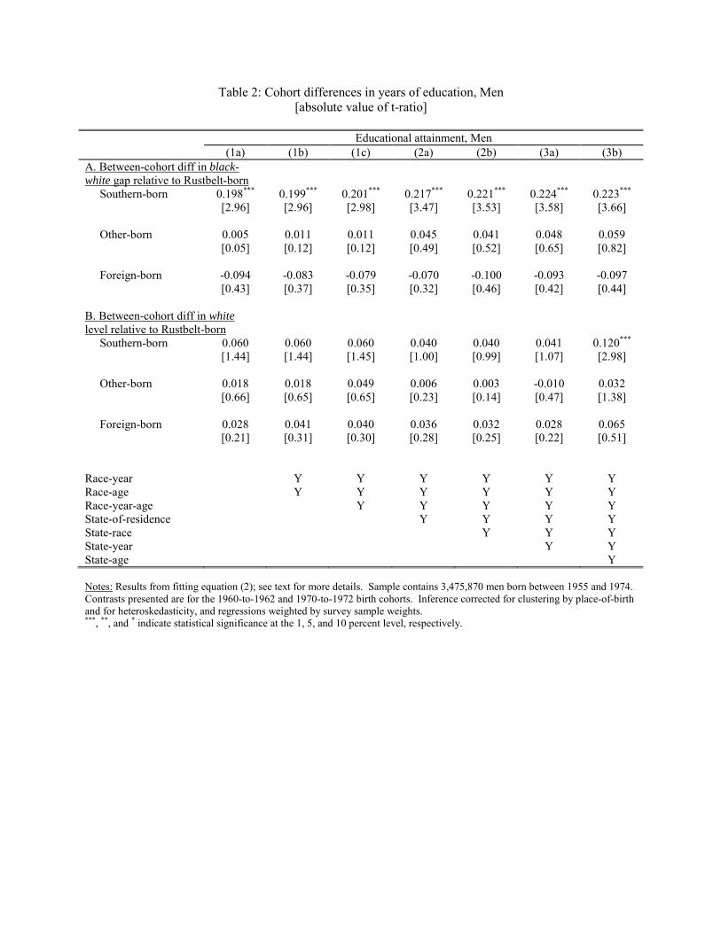
Table 2: Cohort differences in years of education, Men [absolute value of t-ratio]

Educational attainment, Men (1a) (1b) (1c) (2a) (2b) (3a) (3b) A. Between-cohort diff in black-white gap relative to Rustbelt-born

Southern-born 0.198*** 0.199*** 0.201*** 0.217*** 0.221*** 0.224*** 0.223***

[2.96] [2.96] [2.98] [3.47] [3.53] [3.58] [3.66] Other-born 0.005 0.011 0.011 0.045 0.041 0.048 0.059 [0.05] [0.12] [0.12] [0.49] [0.52] [0.65] [0.82] Foreign-born -0.094 -0.083 -0.079 -0.070 -0.100 -0.093 -0.097 [0.43] [0.37] [0.35] [0.32] [0.46] [0.42] [0.44] B. Between-cohort diff in white level relative to Rustbelt-born

Southern-born 0.060 0.060 0.060 0.040 0.040 0.041 0.120***

[1.44] [1.44] [1.45] [1.00] [0.99] [1.07] [2.98] Other-born 0.018 0.018 0.049 0.006 0.003 -0.010 0.032 [0.66] [0.65] [0.65] [0.23] [0.14] [0.47] [1.38] Foreign-born 0.028 0.041 0.040 0.036 0.032 0.028 0.065 [0.21] [0.31] [0.30] [0.28] [0.25] [0.22] [0.51] Race-year Y Y Y Y Y Y Race-age Y Y Y Y Y Y Race-year-age Y Y Y Y Y State-of-residence Y Y Y Y State-race Y Y Y State-year Y Y State-age Y Notes: Results from fitting equation (2); see text for more details. Sample contains 3,475,870 men born between 1955 and 1974. Contrasts presented are for the 1960-to-1962 and 1970-to-1972 birth cohorts. Inference corrected for clustering by place-of-birth and for heteroskedasticity, and regressions weighted by survey sample weights. ***, **, and * indicate statistical significance at the 1, 5, and 10 percent level, respectively.

Table 3: Cohort differences in college attendance, Men [absolute value of t-ratio]

Probability of college, Men (1a) (1b) (1c) (2a) (2b) (3a) (3b) A. Between-cohort diff in black-white gap relative to Rustbelt-born

Southern-born 0.053*** 0.053*** 0.053*** 0.056*** 0.057*** 0.057*** 0.056***

[4.01] [4.00] [4.03] [4.63] [4.74] [4.73] [4.57] Other-born 0.011 0.012 0.012 0.018 0.017 0.021 0.025 [0.65] [0.68] [0.69] [1.10] [1.18] [1.42] [1.64] B. Between-cohort diff in white level relative to Rustbelt-born

Southern-born 0.005 0.005 0.005 0.002 0.002 0.001 0.014**

[0.79] [0.79] [0.80] [0.28] [0.27] [0.19] [2.04] Other-born 0.002 0.002 0.002 -0.001 -0.001 -0.003 0.005 [0.25] [0.26] [0.26] [0.12] [0.16] [0.42] [0.86] Race-year Y Y Y Y Y Y Race-age Y Y Y Y Y Y Race-year-age Y Y Y Y Y State-of-residence Y Y Y Y State-race Y Y Y State-year Y Y State-age Y Notes: See notes to Table 2 and text for more details. Dependent variable is an indicator equal to one if the individual attained at least some college education. ***, **, and * indicate statistical significance at the 1, 5, and 10 percent level, respectively.

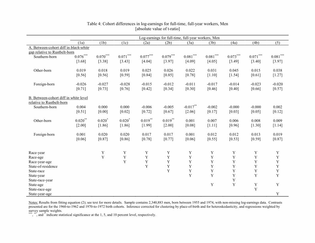
Table 4: Cohort differences in log-earnings for full-time, full-year workers, Men [absolute value of t-ratio]

Log-earnings for full-time, full-year workers, Men (1a) (1b) (1c) (2a) (2b) (3a) (3b) (4a) (4b) (5) A. Between-cohort diff in black-white gap relative to Rustbelt-born

Southern-born 0.076*** 0.070*** 0.071*** 0.077*** 0.079*** 0.081*** 0.081*** 0.073*** 0.071*** 0.081***

[3.68] [3.38] [3.43] [4.04] [3.97] [4.09] [4.05] [3.49] [3.40] [3.97] Other-born 0.019 0.018 0.019 0.025 0.026 0.022 0.031 0.045 0.015 0.038 [0.56] [0.56] [0.59] [0.84] [0.85] [0.78] [1.10] [1.54] [0.61] [1.27] Foreign-born -0.026 -0.027 -0.028 -0.015 -0.012 -0.011 -0.017 -0.014 -0.023 -0.020 [0.71] [0.73] [0.76] [0.42] [0.34] [0.30] [0.46] [0.40] [0.66] [0.57] B. Between-cohort diff in white level relative to Rustbelt-born

Southern-born 0.004 0.000 0.000 -0.006 -0.005 -0.017** -0.002 -0.000 -0.000 0.002 [0.51] [0.00] [0.02] [0.72] [0.67] [2.06] [0.17] [0.03] [0.05] [0.12] Other-born 0.020** 0.020* 0.020* 0.019** 0.019** 0.001 0.007 0.006 0.008 0.009 [2.00] [1.86] [1.86] [1.99] [2.00] [0.08] [1.11] [0.96] [1.30] [1.14] Foreign-born 0.001 0.020 0.020 0.017 0.017 0.001 0.012 0.012 0.013 0.019 [0.06] [0.87] [0.86] [0.78] [0.77] [0.06] [0.55] [0.53] [0.59] [0.87] Race-year Y Y Y Y Y Y Y Y Y Race-age Y Y Y Y Y Y Y Y Y Race-year-age Y Y Y Y Y Y Y Y State-of-residence Y Y Y Y Y Y Y State-race Y Y Y Y Y Y State-year Y Y Y Y Y State-race-year Y State-age Y Y Y Y State-race-age Y State-year-age Y Notes: Results from fitting equation (2); see text for more details. Sample contains 2,340,883 men, born between 1955 and 1974, with non-missing log-earnings data. Contrasts presented are for the 1960-to-1962 and 1970-to-1972 birth cohorts. Inference corrected for clustering by place-of-birth and for heteroskedasticity, and regressions weighted by survey sample weights. ***, **, and * indicate statistical significance at the 1, 5, and 10 percent level, respectively.

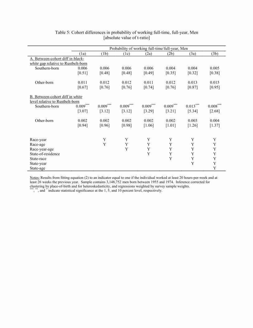
Table 5: Cohort differences in probability of working full-time, full-year, Men [absolute value of t-ratio]

Probability of working full-time/full-year, Men (1a) (1b) (1c) (2a) (2b) (3a) (3b) A. Between-cohort diff in black-white gap relative to Rustbelt-born

Southern-born 0.006 0.006 0.006 0.006 0.004 0.004 0.005 [0.51] [0.48] [0.48] [0.49] [0.35] [0.32] [0.38] Other-born 0.011 0.012 0.012 0.011 0.012 0.013 0.015 [0.67] [0.76] [0.76] [0.74] [0.76] [0.87] [0.95] B. Between-cohort diff in white level relative to Rustbelt-born

Southern-born 0.009*** 0.009*** 0.009*** 0.009*** 0.009*** 0.013*** 0.008***

[3.07] [3.12] [3.12] [3.29] [3.21] [5.34] [2.68] Other-born 0.002 0.002 0.002 0.002 0.002 0.003 0.004 [0.94] [0.96] [0.98] [1.06] [1.01] [1.26] [1.37] Race-year Y Y Y Y Y Y Race-age Y Y Y Y Y Y Race-year-age Y Y Y Y Y State-of-residence Y Y Y Y State-race Y Y Y State-year Y Y State-age Y Notes: Results from fitting equation (2) to an indicator equal to one if the individual worked at least 20 hours-per-week and at least 26 weeks the previous year. Sample contains 3,148,752 men born between 1955 and 1974. Inference corrected for clustering by place-of-birth and for heteroskedasticity, and regressions weighted by survey sample weights. ***, **, and * indicate statistical significance at the 1, 5, and 10 percent level, respectively.

Table 6: Quantile log-earnings results for various samples of Men [absolute value of t-ratio]

Conditional quantiles of log-earnings, Men Full-time, full-year workers All workers All men (missing ln-earnings=0) (1a) (1b) (1c) (2a) (2b) (2c) (3a) (3b) (3c) Between-cohort diff in black-white gap relative to Rustbelt-born

Southern-born 25th percentile 0.037** 0.043*** 0.062*** 0.047*** 0.046** 0.065*** [2.30] [2.67] [3.91] [2.76] [2.51] [3.87] Median 0.089*** 0.075*** 0.069*** 0.074*** 0.078*** 0.067*** [7.01] [5.85] [5.22] [5.92] [6.38] [5.35] 75th percentile 0.072*** 0.076*** 0.081*** 0.074*** 0.079*** 0.097*** 0.065*** 0.073*** 0.073***

[4.75] [5.00] [5.64] [5.40] [5.74] [7.20] [5.09] [5.58] [5.91] Other-born 25th percentile -0.035* -0.016 -0.024 -0.096*** -0.082*** -0.084*** [1.75] [0.82] [1.19] [4.59] [3.66] [4.05] Median -0.004 0.00 -0.015 -0.009 -0.019 -0.034** [0.27] [0.00] [0.93] [0.60] [1.30] [2.25] 75th percentile 0.016 0.002 0.025 0.019 0.001 0.025 0.012 0.006 0.000 [0.83] [0.13] [1.40] [1.11] [0.06] [1.49] [0.75] [0.38] [0.02] Race-year Y Y Y Y Y Y Y Y Y Race-age Y Y Y Y Y Y Race-year-age Y Y Y State-of-residence Y Y Y Sample size 2,340,883 2,340,883 2,340,883 2,657,196 2,657,196 2,657,196 3,523,994 3,523,994 3,523,994 Notes: See text for more details. Sample weights used. In columns 3a-c, the natural logarithm of earnings is set to zero for individuals who either have missing earnings data or have self-reported earnings of zero. Standard errors estimated under the assumption that the residuals are independently and identically distributed. The estimator depends on the reciprocal of the density of the dependent variable evaluated at the quantile of interest (sparsity function). The fitted values for the predicted quantiles and the Epanechnikov kernel were used to estimate the sparsity function. ***, **, and * indicate statistical significance at the 1, 5, and 10 percent level, respectively.

Table 7: Log-earnings results controlling for educational attainment [absolute value of t-ratio]

Log-earnings for full-time, full-year workers, Men (1a) (1b) (1c) (2a) (2b) (2c) (3a) (3b) (3c) A. Between-cohort diff in black-white gap relative to Rustbelt-born

Southern-born 0.076*** 0.056*** 0.053*** 0.079*** 0.059*** 0.056*** 0.082*** 0.062*** 0.058***

[3.70] [3.13] [2.99] [3.99] [3.29] [3.14] [4.08] [3.43] [3.28] Other-born 0.020 0.009 0.009 0.027 0.014 0.014 0.033 0.018 0.018 [0.60] [0.36] [0.37] [0.91] [0.62] [0.64] [1.18] [0.85] [0.88] Foreign-born -0.020 0.008 0.009 -0.006 0.020 0.022 -0.011 0.016 0.018 [0.54] [0.25] [0.28] [0.17] [0.67] [0.74] [0.30] [0.53] [0.60] B. Between-cohort diff in white level relative to Rustbelt-born

Southern-born 0.004 0.004 0.004 -0.005 -0.002 -0.002 -0.001 -0.009 -0.008 [0.49] [0.71] [0.73] [0.67] [0.32] [0.30] [0.13] [1.28] [1.23] Other-born 0.020** 0.018** 0.018** 0.019** 0.018** 0.018** 0.007 0.005 0.005 [1.99] [2.14] [2.14] [1.98] [2.22] [2.21] [1.07] [0.76] [0.75] Foreign-born -0.001 -0.006 -0.006 0.014 0.008 0.008 0.010 0.001 0.000 [0.02] [0.37] [0.38] [0.67] [0.49] [0.48] [0.45] [0.04] [0.03] Education fixed effects Y Y Y Y Y Y Race-education effects Y Y Y Race-year-age Y Y Y Y Y Y State-of-residence-race Y Y Y Y Y Y State-year Y Y Y State-age Y Y Y R-squared 0.034 0.188 0.188 0.094 0.230 0.230 0.097 0.233 0.233 Notes: See notes to Table 4. Sample contains 2,324,807 men, born between 1955 and 1974, with non-missing education data. Inference corrected for clustering by place-of-birth and for heteroskedasticity, and regressions weighted by survey sample weights. ***, **, and * indicate statistical significance at the 1, 5, and 10 percent level, respectively.

Table 8: Log-earnings results controlling for interactions of potential experience with race and state-of-residence [absolute value of t-ratio]

Log-earnings for full-time, full-year workers, Men (1a) (1b) (1c) (2a) (2b) (2c) (3a) (3b) (3c) Between-cohort diff in black-white gap relative to Rustbelt-born

Southern-born 0.057*** 0.058*** 0.060*** 0.059*** 0.060*** 0.062*** 0.062*** 0.059*** 0.061***

[3.49] [3.67] [3.77] [3.71] [3.84] [3.98] [3.53] [3.38] [3.55] Other-born 0.012 0.010 0.010 0.012 0.009 0.010 0.015 0.014 0.015 [0.76] [0.60] [0.63] [0.71] [0.51] [0.57] [0.99] [0.88] [0.98] Foreign-born 0.021 0.012 0.010 0.021 0.012 0.011 0.011 0.006 0.004 [0.67] [0.40] [0.35] [0.66] [0.40] [0.36] [0.35] [0.20] [0.12] Education fixed effects Y Y Y Y Y Y Race-education effects Y Y Y Race-year-age Y Y Y Y Y Y Y Y Y State-of-residence-race Y Y Y Y Y Y Y Y Y State-race-year Y Y Y Y Y Y Y Y Y State-race-experience 4th-order polynomial Y Y Y 8th-order polynomial Y Y Y Experience fixed effects Y Y Y R-squared 0.228 0.238 0.238 0.229 0.238 0.239 0.233 0.242 0.242 Notes: See notes to Table 4 and text for more details. Sample contains 2,324,807 men, born between 1955 and 1974, with non-missing education data. Potential experience is equal to an individual’s age minus year of complete schooling minus six. ***, **, and * indicate statistical significance at the 1, 5, and 10 percent level, respectively.

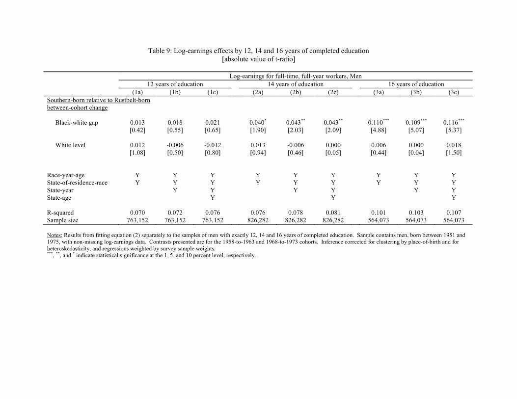
Table 9: Log-earnings effects by 12, 14 and 16 years of completed education [absolute value of t-ratio]

Log-earnings for full-time, full-year workers, Men 12 years of education 14 years of education 16 years of education (1a) (1b) (1c) (2a) (2b) (2c) (3a) (3b) (3c) Southern-born relative to Rustbelt-born between-cohort change

Black-white gap 0.013 0.018 0.021 0.040* 0.043** 0.043** 0.110*** 0.109*** 0.116***

[0.42] [0.55] [0.65] [1.90] [2.03] [2.09] [4.88] [5.07] [5.37] White level 0.012 -0.006 -0.012 0.013 -0.006 0.000 0.006 0.000 0.018 [1.08] [0.50] [0.80] [0.94] [0.46] [0.05] [0.44] [0.04] [1.50] Race-year-age Y Y Y Y Y Y Y Y Y State-of-residence-race Y Y Y Y Y Y Y Y Y State-year Y Y Y Y Y Y State-age Y Y Y R-squared 0.070 0.072 0.076 0.076 0.078 0.081 0.101 0.103 0.107 Sample size 763,152 763,152 763,152 826,282 826,282 826,282 564,073 564,073 564,073 Notes: Results from fitting equation (2) separately to the samples of men with exactly 12, 14 and 16 years of completed education. Sample contains men, born between 1951 and 1975, with non-missing log-earnings data. Contrasts presented are for the 1958-to-1963 and 1968-to-1973 cohorts. Inference corrected for clustering by place-of-birth and for heteroskedasticity, and regressions weighted by survey sample weights. ***, **, and * indicate statistical significance at the 1, 5, and 10 percent level, respectively.

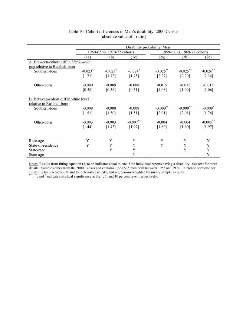
Table 10: Cohort differences in Men’s disability, 2000 Census [absolute value of t-ratio]

Disability probability, Men 1960-62 vs. 1970-72 cohorts 1959-62 vs. 1969-72 cohorts (1a) (1b) (1c) (2a) (2b) (2c) A. Between-cohort diff in black-white gap relative to Rustbelt-born

Southern-born -0.023* -0.023* -0.024* -0.025** -0.025** -0.026**

[1.71] [1.72] [1.75] [2.27] [2.29] [2.34] Other-born -0.009 -0.009 -0.008 -0.015 -0.015 -0.015 [0.58] [0.58] [0.51] [1.08] [1.09] [1.06] B. Between-cohort diff in white level relative to Rustbelt-born

Southern-born -0.008 -0.008 -0.008 -0.009** -0.009** -0.009*

[1.51] [1.50] [1.51] [2.01] [2.01] [1.76] Other-born -0.003 -0.003 -0.007** -0.004 -0.004 -0.005**

[1.44] [1.43] [1.97] [1.60] [1.60] [1.97] Race-age Y Y Y Y Y Y State-of-residence Y Y Y Y Y Y State-race Y Y Y Y State-age Y Y Notes: Results from fitting equation (2) to an indicator equal to one if the individual reports having a disability. See text for more details. Sample comes from the 2000 Census and contains 1,668,535 men born between 1955 and 1974. Inference corrected for clustering by place-of-birth and for heteroskedasticity, and regressions weighted by survey sample weights. ***, **, and * indicate statistical significance at the 1, 5, and 10 percent level, respectively.

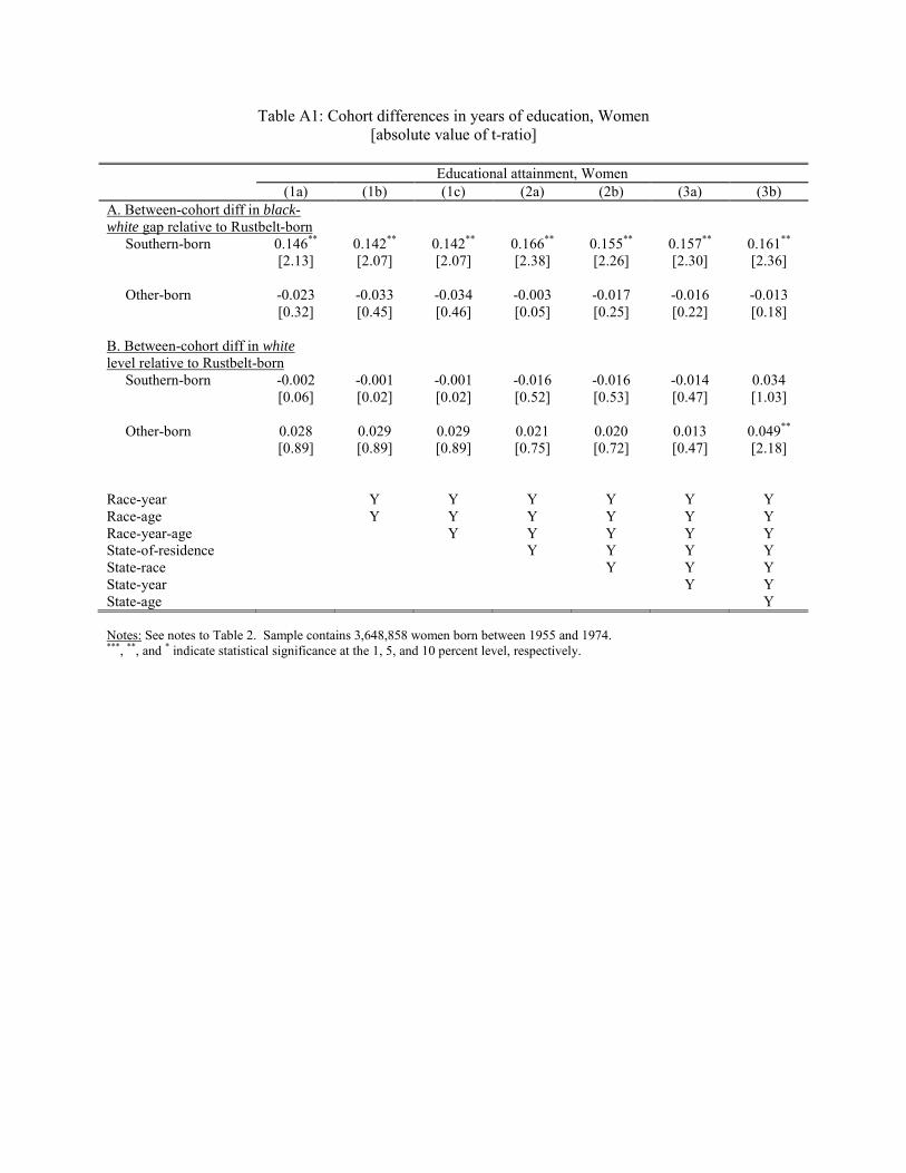
Table A1: Cohort differences in years of education, Women [absolute value of t-ratio]

Educational attainment, Women (1a) (1b) (1c) (2a) (2b) (3a) (3b) A. Between-cohort diff in black-white gap relative to Rustbelt-born

Southern-born 0.146** 0.142** 0.142** 0.166** 0.155** 0.157** 0.161**

[2.13] [2.07] [2.07] [2.38] [2.26] [2.30] [2.36] Other-born -0.023 -0.033 -0.034 -0.003 -0.017 -0.016 -0.013 [0.32] [0.45] [0.46] [0.05] [0.25] [0.22] [0.18] B. Between-cohort diff in white level relative to Rustbelt-born

Southern-born -0.002 -0.001 -0.001 -0.016 -0.016 -0.014 0.034 [0.06] [0.02] [0.02] [0.52] [0.53] [0.47] [1.03] Other-born 0.028 0.029 0.029 0.021 0.020 0.013 0.049**

[0.89] [0.89] [0.89] [0.75] [0.72] [0.47] [2.18] Race-year Y Y Y Y Y Y Race-age Y Y Y Y Y Y Race-year-age Y Y Y Y Y State-of-residence Y Y Y Y State-race Y Y Y State-year Y Y State-age Y Notes: See notes to Table 2. Sample contains 3,648,858 women born between 1955 and 1974. ***, **, and * indicate statistical significance at the 1, 5, and 10 percent level, respectively.

Table A2: Cohort differences in college attendance, Women [absolute value of t-ratio]

Probability of college, Women (1a) (1b) (1c) (2a) (2b) (3a) (3b) A. Between-cohort diff in black-white gap relative to Rustbelt-born

Southern-born 0.032** 0.031** 0.031** 0.035** 0.033** 0.033** 0.033***

[2.02] [1.98] [1.98] [2.19] [2.12] [2.11] [2.07] Other-born 0.006 0.005 0.005 0.010 0.008 0.011 0.015 [0.45] [0.35] [0.32] [0.69] [0.57] [0.81] [1.06] B. Between-cohort diff in white level relative to Rustbelt-born

Southern-born 0.003 0.003 0.003 0.000 0.000 0.002 0.012 [0.32] [0.35] [0.35] [0.05] [0.04] [0.28] [1.63] Other-born -0.002 -0.002 -0.002 -0.004 -0.004 -0.002 0.008 [0.20] [0.18] [0.19] [0.38] [0.40] [0.26] [1.12] Race-year Y Y Y Y Y Y Race-age Y Y Y Y Y Y Race-year-age Y Y Y Y Y State-of-residence Y Y Y Y State-race Y Y Y State-year Y Y State-age Y Notes: See notes to Table A1. Dependent variable is an indicator equal to one if the individual attained at least some college education. ***, **, and * indicate statistical significance at the 1, 5, and 10 percent level, respectively.

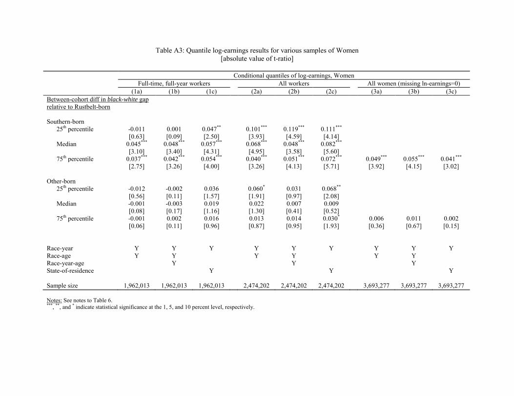
Table A3: Quantile log-earnings results for various samples of Women [absolute value of t-ratio]

Conditional quantiles of log-earnings, Women Full-time, full-year workers All workers All women (missing ln-earnings=0) (1a) (1b) (1c) (2a) (2b) (2c) (3a) (3b) (3c) Between-cohort diff in black-white gap relative to Rustbelt-born

Southern-born 25th percentile -0.011 0.001 0.047** 0.101*** 0.119*** 0.111*** [0.63] [0.09] [2.50] [3.93] [4.59] [4.14] Median 0.045*** 0.048*** 0.057*** 0.068*** 0.048*** 0.082*** [3.10] [3.40] [4.31] [4.95] [3.58] [5.60] 75th percentile 0.037*** 0.042*** 0.054*** 0.040*** 0.051*** 0.072*** 0.049*** 0.055*** 0.041***

[2.75] [3.26] [4.00] [3.26] [4.13] [5.71] [3.92] [4.15] [3.02] Other-born 25th percentile -0.012 -0.002 0.036 0.060* 0.031 0.068** [0.56] [0.11] [1.57] [1.91] [0.97] [2.08] Median -0.001 -0.003 0.019 0.022 0.007 0.009 [0.08] [0.17] [1.16] [1.30] [0.41] [0.52] 75th percentile -0.001 0.002 0.016 0.013 0.014 0.030* 0.006 0.011 0.002 [0.06] [0.11] [0.96] [0.87] [0.95] [1.93] [0.36] [0.67] [0.15] Race-year Y Y Y Y Y Y Y Y Y Race-age Y Y Y Y Y Y Race-year-age Y Y Y State-of-residence Y Y Y Sample size 1,962,013 1,962,013 1,962,013 2,474,202 2,474,202 2,474,202 3,693,277 3,693,277 3,693,277 Notes: See notes to Table 6. ***, **, and * indicate statistical significance at the 1, 5, and 10 percent level, respectively.

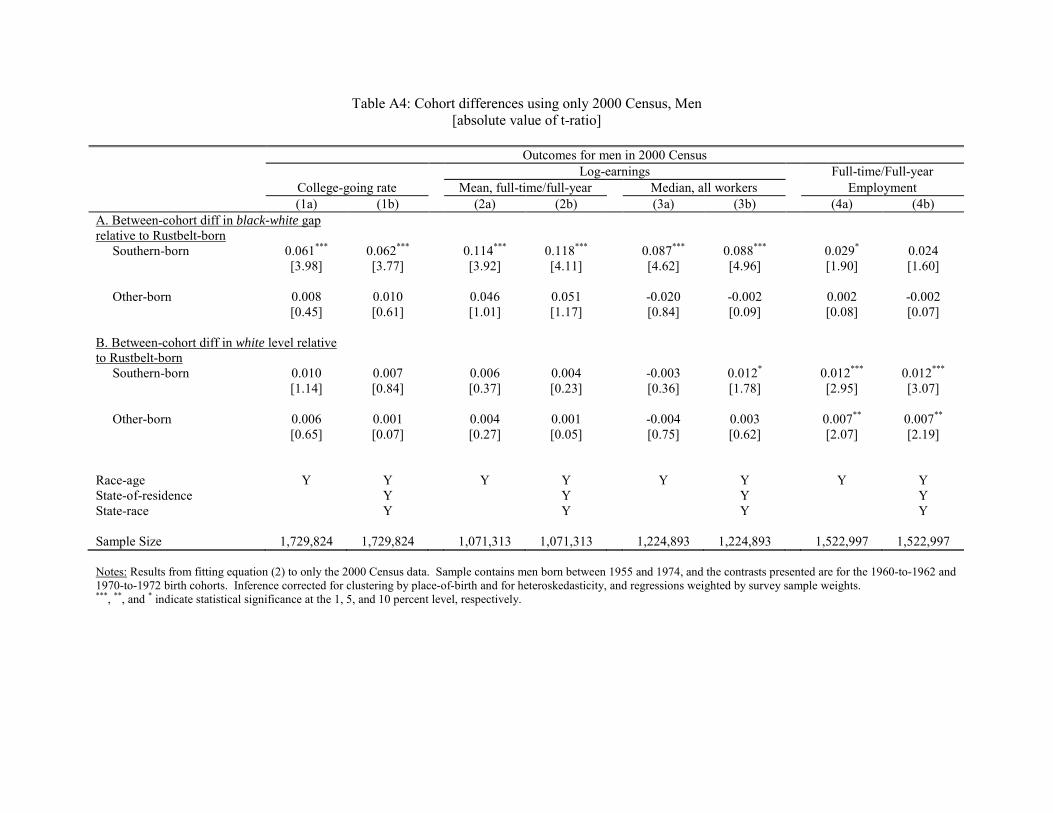
Table A4: Cohort differences using only 2000 Census, Men [absolute value of t-ratio]

Outcomes for men in 2000 Census Log-earnings Full-time/Full-year College-going rate Mean, full-time/full-year Median, all workers Employment (1a) (1b) (2a) (2b) (3a) (3b) (4a) (4b) A. Between-cohort diff in black-white gap relative to Rustbelt-born

Southern-born 0.061*** 0.062*** 0.114*** 0.118*** 0.087*** 0.088*** 0.029* 0.024 [3.98] [3.77] [3.92] [4.11] [4.62] [4.96] [1.90] [1.60] Other-born 0.008 0.010 0.046 0.051 -0.020 -0.002 0.002 -0.002 [0.45] [0.61] [1.01] [1.17] [0.84] [0.09] [0.08] [0.07] B. Between-cohort diff in white level relative to Rustbelt-born

Southern-born 0.010 0.007 0.006 0.004 -0.003 0.012* 0.012*** 0.012***

[1.14] [0.84] [0.37] [0.23] [0.36] [1.78] [2.95] [3.07] Other-born 0.006 0.001 0.004 0.001 -0.004 0.003 0.007** 0.007**

[0.65] [0.07] [0.27] [0.05] [0.75] [0.62] [2.07] [2.19] Race-age Y Y Y Y Y Y Y Y State-of-residence Y Y Y Y State-race Y Y Y Y Sample Size 1,729,824 1,729,824 1,071,313 1,071,313 1,224,893 1,224,893 1,522,997 1,522,997 Notes: Results from fitting equation (2) to only the 2000 Census data. Sample contains men born between 1955 and 1974, and the contrasts presented are for the 1960-to-1962 and 1970-to-1972 birth cohorts. Inference corrected for clustering by place-of-birth and for heteroskedasticity, and regressions weighted by survey sample weights. ***, **, and * indicate statistical significance at the 1, 5, and 10 percent level, respectively.

Figure 1: Difference in black-white education gaps between Southern- and Rustbelt-born, Men A. Years of education

B. Probability of some college education or more

-0.3

-0.2

-0.1

0

0.1

0.2

0.3

0.4

0.5

0.6

1951 1953 1955 1957 1959 1961 1963 1965 1967 1969 1971 1973 1975 1977

Birth Year

Sou

th-R

ustb

elt d

iff in

bla

ck-w

hite

edu

catio

n ga

p

no controls + race-age, state-of-residence

-0.1

-0.08

-0.06

-0.04

-0.02

0

0.02

0.04

0.06

0.08

1951 1953 1955 1957 1959 1961 1963 1965 1967 1969 1971 1973 1975 1977

Birth Year

Sou

th-R

ustb

elt d

iff in

bla

ck-w

hite

Col

lege

gap

no controls + race-age, state-of-residence

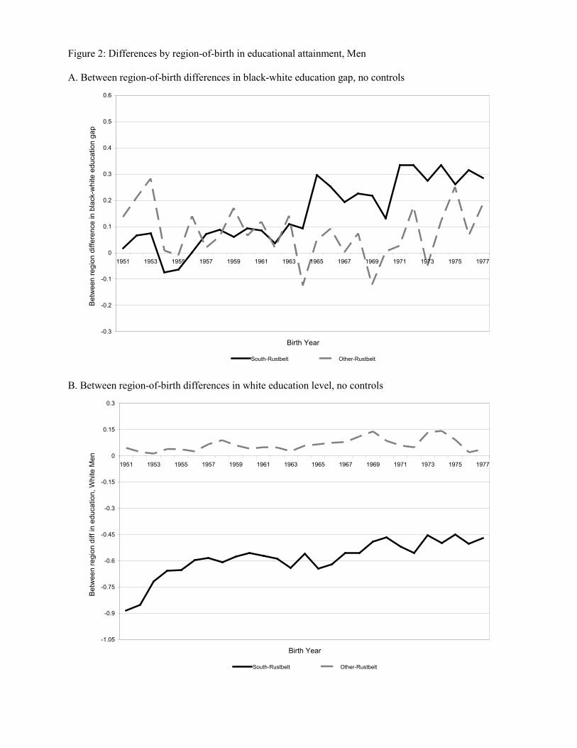
Figure 2: Differences by region-of-birth in educational attainment, Men A. Between region-of-birth differences in black-white education gap, no controls

B. Between region-of-birth differences in white education level, no controls

-0.3

-0.2

-0.1

0

0.1

0.2

0.3

0.4

0.5

0.6

1951 1953 1955 1957 1959 1961 1963 1965 1967 1969 1971 1973 1975 1977

Birth Year

Bet

wee

n re

gion

diff

eren

ce in

bla

ck-w

hite

edu

catio

n ga

p

South-Rustbelt Other-Rustbelt

-1.05

-0.9

-0.75

-0.6

-0.45

-0.3

-0.15

0

0.15

0.3

1951 1953 1955 1957 1959 1961 1963 1965 1967 1969 1971 1973 1975 1977

Birth Year

Bet

wee

n re

gion

diff

in e

duca

tion,

Whi

te M

en

South-Rustbelt Other-Rustbelt

Figure 3: Differences by region-of-birth in probability of going to college, Men A. Between region-of-birth differences in black-white college-going gap, no controls

B. Between region-of-birth differences in white college-going rate, no controls

-0.1

-0.08

-0.06

-0.04

-0.02

0

0.02

0.04

0.06

0.08

1951 1953 1955 1957 1959 1961 1963 1965 1967 1969 1971 1973 1975 1977

Birth Year

Bet

wee

n re

gion

diff

eren

ce in

bla

ck-w

hite

Col

lege

gap

South-Rustbelt Other-Rustbelt

-0.15

-0.12

-0.09

-0.06

-0.03

0

0.03

0.06

1951 1953 1955 1957 1959 1961 1963 1965 1967 1969 1971 1973 1975 1977

Birth Year

Bet

wee

n re

gion

diff

in C

olle

ge, W

hite

Men

South-Rustbelt Other-Rustbelt

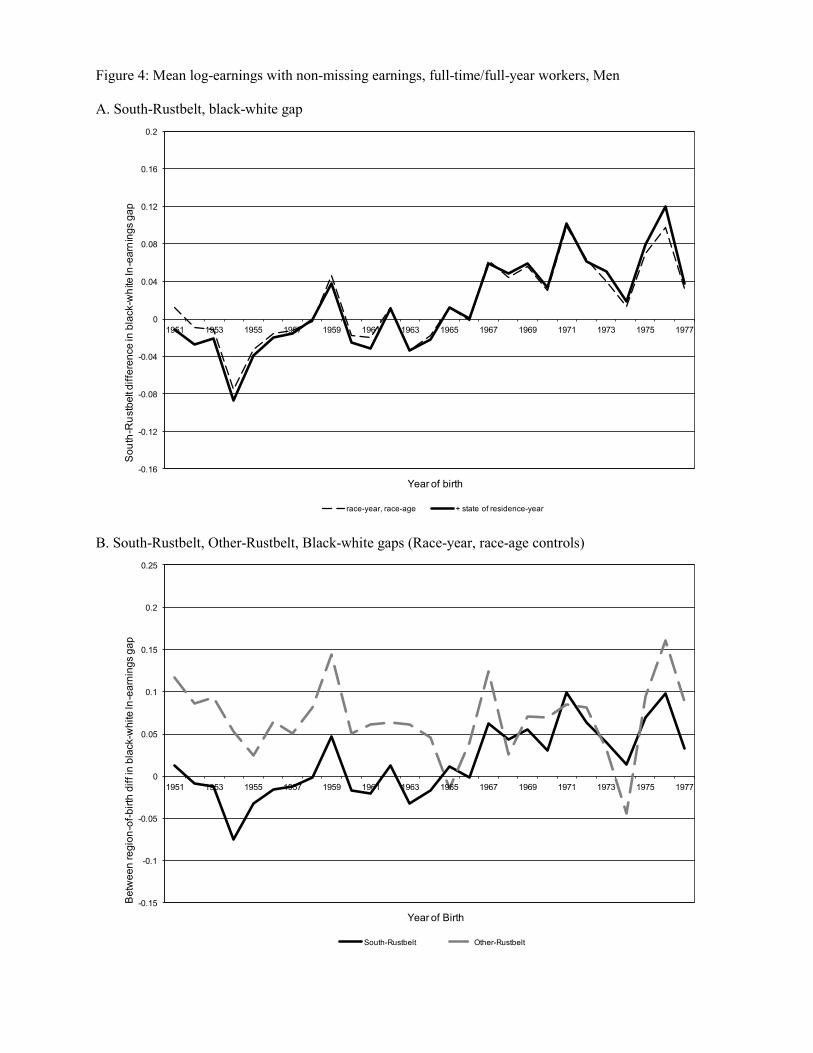
Figure 4: Mean log-earnings with non-missing earnings, full-time/full-year workers, Men A. South-Rustbelt, black-white gap

B. South-Rustbelt, Other-Rustbelt, Black-white gaps (Race-year, race-age controls)

-0.16

-0.12

-0.08

-0.04

0

0.04

0.08

0.12

0.16

0.2

1951 1953 1955 1957 1959 1961 1963 1965 1967 1969 1971 1973 1975 1977

Sou

th-R

ustb

elt d

iffer

ence

in b

lack

-whi

te ln

-ear

ning

s ga

p

Year of birth

race-year, race-age + state of residence-year

-0.15

-0.1

-0.05

0

0.05

0.1

0.15

0.2

0.25

1951 1953 1955 1957 1959 1961 1963 1965 1967 1969 1971 1973 1975 1977

Bet

wee

n re

gion

-of-b

irth

diff

in b

lack

-whi

te ln

-ear

ning

s ga

p

Year of Birth

South-Rustbelt Other-Rustbelt

C. South-Rustbelt, Other-Rustbelt, Black-white gaps (Race-year, race-age, state-year controls)

D. South-Rustbelt, Other-Rustbelt, White differences (Race-year, race-age, state-year controls)

-0.2

-0.15

-0.1

-0.05

0

0.05

0.1

0.15

0.2

1951 1953 1955 1957 1959 1961 1963 1965 1967 1969 1971 1973 1975 1977

Bet

wee

n re

gion

-of-b

irth

diff

in b

lack

-whi

te ln

-ear

ning

s ga

p

Year of Birth

South-Rustbelt Other-Rustbelt

-0.2

-0.16

-0.12

-0.08

-0.04

0

0.04

0.08

0.12

1951 1953 1955 1957 1959 1961 1963 1965 1967 1969 1971 1973 1975 1977

Bet

wee

n re

gion

-of-b

irth

diffe

renc

e in

Whi

te ln

-ear

ning

s

Year of Birth

South-Rustbelt Other-Rustbelt

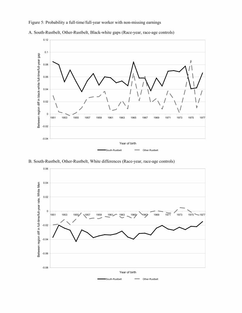
Figure 5: Probability a full-time/full-year worker with non-missing earnings A. South-Rustbelt, Other-Rustbelt, Black-white gaps (Race-year, race-age controls)

B. South-Rustbelt, Other-Rustbelt, White differences (Race-year, race-age controls)

-0.04

-0.02

0

0.02

0.04

0.06

0.08

0.1

0.12

1951 1953 1955 1957 1959 1961 1963 1965 1967 1969 1971 1973 1975 1977

Year of birth

Bet

wee

n re

gion

diff

in b

lack

-whi

te fu

ll-tim

e/fu

ll-ye

ar g

ap

South-Rustbelt Other-Rustbelt

-0.08

-0.06

-0.04

-0.02

0

0.02

0.04

0.06

1951 1953 1955 1957 1959 1961 1963 1965 1967 1969 1971 1973 1975 1977

Year of birth

Bet

wee

n re

gion

diff

in fu

ll-tim

e/fu

ll-ye

ar ra

te, W

hite

Men

South-Rustbelt Other-Rustbelt

Figure 6: Median log-earnings with non-missing earnings, all workers, Men A. South-Rustbelt, Other-Rustbelt, Black-white gaps (race-by-year effects, state-of-residence effects)

B. South-Rustbelt, Other-Rustbelt, White differences (race-by-year effects, state-of-residence effects)

-0.16

-0.12

-0.08

-0.04

0

0.04

0.08

0.12

0.16

0.2

1956 1957 1958 1959 1960 1961 1962 1963 1964 1965 1966 1967 1968 1969 1970 1971 1972 1973 1974

Year of Birth

Bla

ck-w

hite

gap

in m

edia

n ln

-ear

ning

s, re

lativ

e to

Rus

tbel

t-bor

n

South-born Other-born

-0.2

-0.16

-0.12

-0.08

-0.04

0

0.04

0.08

0.12

0.16

1956 1957 1958 1959 1960 1961 1962 1963 1964 1965 1966 1967 1968 1969 1970 1971 1972 1973 1974

Year of Birth

Whi

te m

edia

n ln

-ear

ning

s, re

lativ

e to

Rus

tbel

t-bor

n

South-born Other-born

Figure 7: Scatter plots of between-cohort changes in racial gaps (22 states) A. Change in gaps in College-going rate and PNMR

B. Change in gaps in Log-earnings and PNMR

-0.04

-0.02

0

0.02

0.04

0.06

0.08

-12 -11 -10 -9 -8 -7 -6 -5 -4 -3 -2 -1 0 1 2

Black-white PNMR gap (1969-74 minus 1959-64)

Bla

ck-w

hite

col

lege

-goi

ng g

ap (1

968-

73 m

inus

195

8-63

)

South Border States Rustbelt

y = –0.0193 – 0.0076∙x, R-squared=0.673 [4.15] [9.01]

-0.1

-0.05

0

0.05

0.1

0.15

0.2

-12 -11 -10 -9 -8 -7 -6 -5 -4 -3 -2 -1 0 1 2

Black-white PNMR gap (1969-74 minus 1959-64)

Bla

ck-w

hite

log-

earn

ings

gap

(196

8-73

min

us 1

958-

63)

South Border States Rustbelt

y = –0.0083 – 0.0113∙x, R-squared=0.474 [0.53] [3.82]

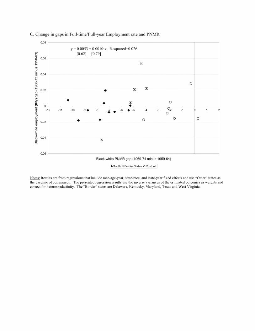
C. Change in gaps in Full-time/Full-year Employment rate and PNMR

Notes: Results are from regressions that include race-age-year, state-race, and state-year fixed effects and use “Other” states as the baseline of comparison. The presented regression results use the inverse variances of the estimated outcomes as weights and correct for heteroskedasticity. The “Border” states are Delaware, Kentucky, Maryland, Texas and West Virginia.

-0.06

-0.04

-0.02

0

0.02

0.04

0.06

0.08

-12 -11 -10 -9 -8 -7 -6 -5 -4 -3 -2 -1 0 1 2

Black-white PNMR gap (1969-74 minus 1959-64)

Bla

ck-w

hite

em

ploy

men

t (ft/

fy) g

ap (1

968-

73 m

inus

195

8-63

)

South Border States Rustbelt

y = 0.0053 + 0.0010∙x, R-squared=0.026 [0.62] [0.79]

Figure 8: Mean log-earnings by age for men employed full-time/full-year, by region-of-birth

A. Black-white log-earnings gap in 1990 Census

B. Change in black-white log-earnings gap between 1990 and 2000 Censuses

-0.45

-0.4

-0.35

-0.3

-0.25

-0.2

-0.15

-0.1

-0.0526 27 28 29 30 31 32 33 34 35 36 37 38 39 40 41 42 43 44

Bla

ck-w

hite

gap

in lo

g-ea

rnin

gs in

199

0

Age

South-born

Rustbelt- andOther-born

-0.2

-0.16

-0.12

-0.08

-0.04

0

0.04

0.08

0.12

0.16

26 27 28 29 30 31 32 33 34 35 36 37 38 39 40 41 42 43 44

Cha

nge

in b

lack

-whi

te lo

g-ea

rnin

gs g

ap fr

om 1

990

to 2

000

Age

South-born

Rustbelt- andOther-born

C. Change in white log-earnings between 1990 and 2000 Censuses

Notes: The South-born and Rustbelt-and-Other-born samples of full-time, full-year workers (with non-missing log-earnings) consist respectively of 391,555 and 1,528,558 observations. In Panel A the sampling errors are roughly 0.018 to 0.020 for the South-born and 0.019 to 0.025 for the Rustbelt- and Other-born. In Panel B they are 0.028 to 0.030 for the South-born and 0.029 to 0.034 for the Rustbelt- and Other-born. In Panel C they are 0.012 to 0.014 for the South-born and 0.007 for the Rustbelt- and Other-born.

-0.09

-0.06

-0.03

0

0.03

0.06

0.09

0.12

26 27 28 29 30 31 32 33 34 35 36 37 38 39 40 41 42 43 44

Cha

nge

in lo

g-ea

rnin

gs fr

om 1

990

to 2

000,

whi

te m

en

Age

South-born

Rustbelt- andOther-born

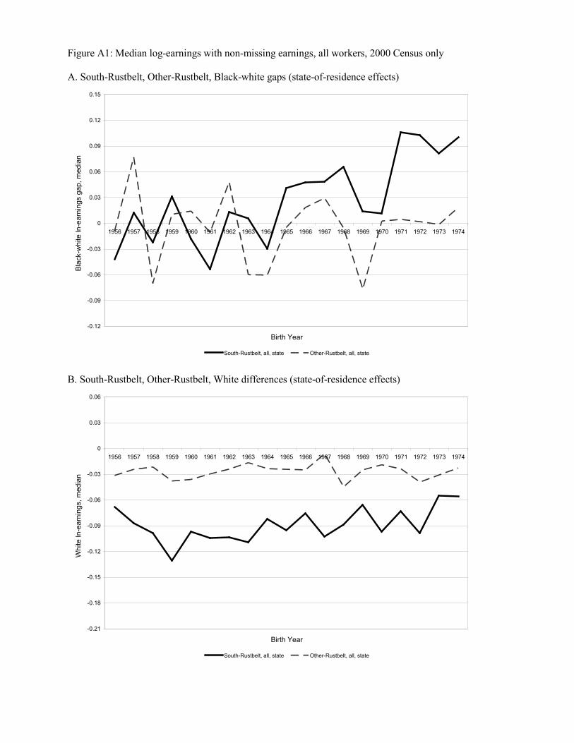
Figure A1: Median log-earnings with non-missing earnings, all workers, 2000 Census only A. South-Rustbelt, Other-Rustbelt, Black-white gaps (state-of-residence effects)

B. South-Rustbelt, Other-Rustbelt, White differences (state-of-residence effects)

-0.12

-0.09

-0.06

-0.03

0

0.03

0.06

0.09

0.12

0.15

1956 1957 1958 1959 1960 1961 1962 1963 1964 1965 1966 1967 1968 1969 1970 1971 1972 1973 1974

Birth Year

Bla

ck-w

hite

ln-e

arni

ngs

gap,

med

ian

South-Rustbelt, all, state Other-Rustbelt, all, state

-0.21

-0.18

-0.15

-0.12

-0.09

-0.06

-0.03

0

0.03

0.06

1956 1957 1958 1959 1960 1961 1962 1963 1964 1965 1966 1967 1968 1969 1970 1971 1972 1973 1974

Birth Year

Whi

te ln

-ear

ning

s, m

edia

n

South-Rustbelt, all, state Other-Rustbelt, all, state

Figure A2: Male black-white ratio of median income, all workers A. United States, 1948 to 2011

B. South and Northeast, 1953 to 2011

0.4

0.45

0.5

0.55

0.6

0.65

0.7

0.75

0.8Bl

ack-

Whi

te R

atio

of I

ncom

e (a

ll wor

kers

aged

14-

15+)

Year

Median income, Men

0.2

0.3

0.4

0.5

0.6

0.7

0.8

0.9

Mal

e Bl

ack-

Whi

te R

atio

of M

edia

n In

com

e (a

ll w

orke

rs)

Year

South

Northeast

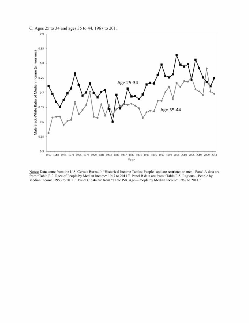
C. Ages 25 to 34 and ages 35 to 44, 1967 to 2011

Notes: Data come from the U.S. Census Bureau’s “Historical Income Tables: People” and are restricted to men. Panel A data are from “Table P-2. Race of People by Median Income: 1947 to 2011.” Panel B data are from “Table P-5. Regions—People by Median Income: 1953 to 2011.” Panel C data are from “Table P-8. Age—People by Median Income: 1967 to 2011.”

0.5

0.55

0.6

0.65

0.7

0.75

0.8

0.85

0.9

1967 1969 1971 1973 1975 1977 1979 1981 1983 1985 1987 1989 1991 1993 1995 1997 1999 2001 2003 2005 2007 2009 2011

Mal

e Bl

ack-

Whi

te R

atio

of M

edia

n In

com

e (a

ll w

orke

rs)

Year

Age 25-34

Age 35-44

Figure A3: Change in racial gap by age and region-of-residence, men employed full-time/full-year

A. Change in black-white log-earnings gap between 1990 and 2000 for residents of South

B. Change in racial gap for South-born living in non-South and non-South-born living in South

Notes: See text for the regression specifications used to generate the figures and the sampling errors. Non-South consists of the states of the Rustbelt and Other regions. Border states included in the analysis but with effects that are not presented.

-0.06

-0.03

0

0.03

0.06

0.09

0.12

0.15

0.18

0.21

26 27 28 29 30 31 32 33 34 35 36 37 38 39 40 41 42 43 44

Cha

nge

in b

lack

-whi

te lo

g-ea

rnin

gs g

ap fr

om 1

990

to 2

000

Age

All South residents South-born, South residents

-0.4

-0.3

-0.2

-0.1

0

0.1

0.2

0.3

0.4

26 27 28 29 30 31 32 33 34 35 36 37 38 39 40 41 42 43 44

Cha

nge

in b

lack

-whi

te lo

g-ea

rnin

gs g

ap fr

om 1

990

to 2

000

Age

Non-South residentsborn in South

South residentsborn in Non-South