EACLIPSE RESEARCH ACTIVITIES AND RESULTS, 2008-09 Introduction to Project Research Activities The second year of the project, “Dynamic Interactions among People, Livestock, and Savanna Ecosystems under Climate Change” (commonly known as EACLIPSE for East Africa Climate-Land Interaction Project in Savanna Ecosystems) was focused on a continuation of the fieldwork and statistical analyses started in Year 1, and the start of modeling activities that will eventually link the various threads of the research together through space and time. The project is working towards understanding the dynamics between the coupled human and biophysical systems in the East African savannas under climate change. The project covers the savannas of Kenya and Tanzania, with fieldwork and high resolution modeling and analysis in agro-pastoral sites in northern Tanzania and southern Kenya. The threads of the research include analysis of the human land management system at the household, community and regional levels, analysis of the ecological system from plant species to land cover types, and analysis of climate from the station to the regional level. Various types of data and information are providing some information on the relations of changes in climate, humans and ecological systems such as remote sensing data and perceptions of local people. The modeling will help quantify and extend the interactions, as well. The main research activities of Year 2 of the project, include:

1. the continuation of ecological, socioeconomic and land use change fieldwork in Kenya and Tanzania,

2. analysis of remote sensing data and meteorological station data to identify temporal and spatial trends and patterns in climate and vegetation, and

3. regional climate modeling and coupled climate/ vegetation and surface water modeling. These various activities were conducted by scientists and students at the University of Dar es Salaam (UDSM) in Tanzania, the International Livestock Research Institute (ILRI) in Kenya, and Virginia Polytechnic University (VPI),. Ohio University (OU) and Michigan State University (MSU) in the U.S. Coordination was assisted by holding bi-monthly meetings at Michigan State University with OU and VPI members joining by telephone or Skype. Olson, the project’s PI, made around five visits to Tanzania and Kenya over the course of the year (some trips funded by other sources). A workshop bringing together all those conducting field work in Kenya and Tanzania was held in July 2008 in Mto wa Mbu, Tanzania (near our field site) to discuss preliminary findings and statistical analysis approaches. This cross-site comparison workshop occurred at the same time as the EACLIPSE education group (Michigan teachers, Tanzanian teacher-educators, MSU education specialists) was meeting to prepare teaching modules, so the education group was able to see the field work results first hand from the researchers. These and other educational activities are described in the Training section of this report. An unfortunate situation of a three-year long prolonged drought in the study areas has affected the ability of both the ecological and socioeconomic field teams to complete their data collection. The ecological teams in both Kenya and Tanzania collected data in their plots twice (once in the dry season and once in what should have been the wet season) but because of the drought, very little especially annual and grass species were left to count. We probably need to return to the

1

plots a third time after the rains start (hopefully in November). The team conducting the household survey was able to collect some data in the Kenyan site but before we could finish, households started dispersing across wide areas, many over 50 kilometers away, to search for water and forage for their animals. We still need to complete some household surveys in Kenya, and all of those needed in Tanzania. The socioeconomic qualitative information collection (community mapping, wealth ranking, etc.) was completed in Kenya but not all the villages were completed in Tanzania before people started dispersing. It is an awkward situation to request people to stay and answer our questions when they are so busy and preoccupied. Methodology of Field Data Collection The approach of the project is necessarily multi-faceted and complex due to the nature of the questions being addressed concerning the interaction over space and time of climate, vegetation, human land management and the wider socioeconomic system. The project has adopted the following principles in developing its methodology:

1. Triangulation of data / information from different sources. For example, analyze information on changing vegetation information from a) remote sensing/ NDVI, LUCC from air photos and imagery, b) community mapping and timeline exercises, c) community and household surveys, and d) vegetation plot analysis.

2. Collect similar information at different spatial scales (household, community, site or “box”, and regional. These could include, for example, plant species/ plant composition/ and biome information at different scales.

3. In the data analysis, focus on the causal or impact linkages between changes in climate, vegetation and human livelihoods. Work towards understanding the relative importance of each affecting the other (especially the relative influence of climate and land use on vegetation).

Much of the data and information being analyzed comes from other sources, either from prior fieldwork of the researchers or others, from publicly available data, and from other secondary sources. The field work sites, for example, were chosen in part because of existing data and information in those areas. Nevertheless, it was decided that some new data did need to be collected to answer the specific questions of this project that require parallel ecological and socioeconomic data and information covering the same locations and time periods, and to permit effective cross-site comparison. Two initial sites were chosen for focused field data collection and high resolution modeling, one in northern Tanzania (Simanjiro District), and one in southern Kenya (Loitokitok District, formerly part of Kajiado District). These two sites are near enough to each other to be within one “box” straddling the Kenya/ Tanzania border for high resolution modeling and remote sensing data analysis (Figure 1). The team would like to include an additional box and fieldwork site, north of Mt. Kenya (Isiolo and Laikipia Districts) if funds and time permit. All sites are in semi-arid savanna areas dominated by agro-pastoralism, and have seen dynamic changes in the past 20 to 30 years. Both have been affected by strong governmental support for wildlife conservation, and have witnessed an increase in the importance of farming by themselves and in-migrants, and erosion of the social and economic basis of the pastoral system. Loitokitok in Kenya is less remote and better linked to the national economy and services, while Simanjiro is more remote. Both have been significantly affected by the recent drought.

2

Fig. 1. Study domain of the EACLIPSE project. Remote sensing analysis and coupled modeling is occurring in all of Kenya and Tanzania, and detailed modeling and fieldwork are occurring in the two “boxes” or sites.

3

Field Data Collection The methodology and sampling strategy for conducting the fieldwork activities were developed in Year 1 of the project, and data sheets and questionnaires tested and finalized in Year 2. A guide summarizing the methodology was prepared and shared among the team members (Olson 2008). To better ensure comparable data collection procedures, the main Kenyan ecological field researcher (Mugatha) and socioeconomic researchers (Smucker, Wangui and Karanja) joined the Tanzanian teams at the start of their fieldwork, and the one socio-economist, Karanja, is leading the household surveys in both Kenya and Tanzania. The Tanzanian ecological team includes Noah, Mwansasu and Yanda, and socioeconomic team includes Mong’ong’o, Olson and two Master’s students. The Kenyan ecological team consists of Mugatha, Said, Maitima and Ogutu, and socioeconomic team is Karanja, Herrero, Smucker and Wangui. Sampling strategy In order to identify the effect of climate and land use on vegetation transects representing a gradient of climate and land use type/ intensity were selected. Some transects cross a climate gradient (e.g., from cool/ moist to hot/ dry) and plots are sampled among the climate types to obtain examples of different land uses (wildlife conservation, wildlife/livestock grazing, and mixed crop/livestock). Where climate doesn’t vary much such as in Simanjiro, the transects cross land use intensity gradients. In all, six transects were chosen in Loitokitok (four near and across the Amboseli National Park and two on the northern slopes of Mt. Kilimanjaro) and four transects were chosen in Simanjiro (starting in Tarangire National Park crossing land uses including the park, a game reserve, grazing, and mixed farming/ grazing) and covering different vegetation types (dominated by grasses, herbaceous plants, shrubs or trees). See Figures 2 and 3 for the locations of the plots. Thirty plots were sampled in Loitokitok and thirty in Simanjiro. The villages near these sites were selected for the socioeconomic information collection. The community level, qualitative work (community mapping, wealth ranking, timelines) was done in each village so that the villagers could provide a historical context and causal interpretation for the data collected by the land use survey and the vegetation plots. Within the villages, a random sample of 30 households in each wealth category was selected for the household survey. Ecological data collection The EACLIPSE ecological fieldwork approach was two-pronged. First, ecological parameters were measured using standard field methods and apparatus to capture variability within and across different land use types. Secondly, historical changes and trends were assessed by use of questionnaires that were administered to livestock keepers and farmers that lived nearest to each plot for more than 40 years. Once a plot starting point was determined, GPS coordinates were taken and the plot was laid 100m in the east direction and 50m in the north direction. There are therefore 8 quadrants or subplots of 25x25m. The plot was assigned a number and a photo of that number taken at diagonal of the plot (north east direction). Herbaceous and grass layer parameters were enumerated in a set of two 1mx1m quadrat laid out within 25mx25m quadrat in each plot (Figure 4). In the 25mx25m quadrants trees and shrubs were sampled. Five most dominant species of trees and shrubs were identified and recorded at each quadrat. See Figure 4 for a list of variables that were collected in each sampling point. In addition to these variables, soil samples were collected in the Tanzanian points. The ecological teams consisted of ecologists, geographers and

4

a botanist, who provided their expertise to identify plant species, describe their environmental requirements, and provide information on plant indicators (of, for example, heavy grazing or recent burning). In addition, an ecological questionnaire was administered to get local historical and contemporary views of vegetation trends such as increase or decrease of species, bush encroachment or opening up, use of fire, and browser population changes over time. Forty questionnaires were administered in Simanjiro, and 30 in Loitokitok.

Fig. 2. Map of the Sampled Plots in Simanjiro, Tanzania.

5

Fig. 3. Map of Sample Plots in Loitokitok, Kenya.

N

50m

25mx25m

1mx1m

E 100m

Fig. 4. Plot and quadant layout

6

Plot size (m) Herbaceous Shrub Tree25x25 (8/plot) Ranked five dominant sp

(grass & herbs•Ranked five dominant sp •Ranked five dominant sp

•Sp count •Sp count •% cover •% cover •Greenness •DBH •Leafyness •Greenness •Burn & age of burn •Leafyness

•Burn & age of burn •Damage, agent & degree, age of damage

1x1m (16/plot) •% cover •% bare ground •Sp count •Ht (m) •% litter •% greenness •Burn •Grazing levl •Types & no. animals in site

Fig. 5. Variables collected at each data point. In both Loitokitok and Simanjiro, the ecological teams have visited the plots to collect data during a dry season and a wet season. The prolonged drought, however, has affected the results. The plots in the “wet” reason were actually drier than they had been earlier (Fig. 6).

Fig. 6. Photos taken of the same plots during the dry and wet season during the ecological fieldwork, Loitokitok, by Mugatha.

7

Photos of wildlife affected by drought taken during fieldwork in Loitokitok, by Mugatha. After the data was collected, it was checked for consistency and accuracy, and species lists forwarded to the botanists for checking. At this point, data entry templates have been created for the three types of data collected – the vegetation plots, the land use survey and the household survey, and the data that has been collected has been entered. Species area curves have been generated for the different land use categories and land forms, and other preliminary analyses conducted. The statistical analysis of the data is on-going. To ensure similar analysis of both sites’ data, the Tanzanian team members will come to Nairobi in October 2009 to meet with the ILRI team members and project PI. As explained above, the drought has affected the field data collection. We may return to the vegetation plots for a third time after it has rained and plants have emerged, and we have not been able to complete the household surveys and community meetings because people have scattered over long distances seeking water and forage for their animals. Data analysis of existing vegetation plot data The EACLIPSE project is also taking advantage of a large, longitudinal database of plant species collected in the Masai Mara National Reserve by WWF’s Maasai Mara Ecological Monitoring Program from July 1989 to December 2003. The data had been collected using a comparable methodology as the EACLIPSE project. An agreement was signed between Ogutu at ILRI and the WWF - Eastern Africa Regional Programme Office permitting ILRI to enter, clean and analyze the data under the EACLIPSE project umbrella. The aim is to conduct an analysis of long-term trends in woody vegetation dynamics. The data are being used to 1) establish spatial and temporal patterns of variability in herbaceous and woody plant species, and 2) evaluate the relative importance of variability in climate, including climatic extremes, fire occurrences and herbivory on the established dynamics in herbaceous and woody vegetation. During the period of this report, the data entry and cleaning was completed, and researchers at ILRI from the University of Groningen, the Netherlands (Bhola), the University of Hohenheim (Anderson) and ILRI (Ogutu) explored various methods of statistically analyzing these data. A suitable statistical model for long-term trends in counts of trees and shrubs should accommodate possibly nonlinear trends for different plots. The model should further allow for non-normality of the tree counts, many zeros and missing counts.

8

We analyzed long-term trends in the monthly counts using a Generalized Linear, Mixed Effects GLMM with a negative binomial error distribution and a log link function of the time series of counts to allow for trend curves for different plots. The trend model included both fixed and random effects. The fixed effects included plot, year, age class and the various interactions and the random part of the model accounted for spatial and temporal autocorrelation in the counts of each plant species in each plot through time and across plots. The model assumed autoregressive error structure. We thus used a spatial power function due to the irregular sampling points and computed the correlation as a function of distance of separation between pairs of sampling points through time. Additional analyses will be explored in the 2009-2010 period:

1) Species turnover in space and time 2) Species abundance distributions 3) Germination and recruitment of woody seedlings and saplings 4) Threshold effects, regime shifts and stable states in woody cover- 5) Allometry, biomass scaling, ecological equivalence - equilibrium vs. non-equilibrium

dynamics. Themes emerging from the ecological fieldwork The savanna vegetation is evolving across the landscape due to both changes in land use and land management, and to changes in the climate. The main changes that have been observed by the researchers and/or by the local herders and farmers, and that will examined in the statistical and remote sensing analyses, include:

1. Bush encroachment in several areas that had been grassland. The reasons given by local people include: prolonged drought, reduced fire incidents that used to promote grass, overgrazing, and cultivation (opening new land).

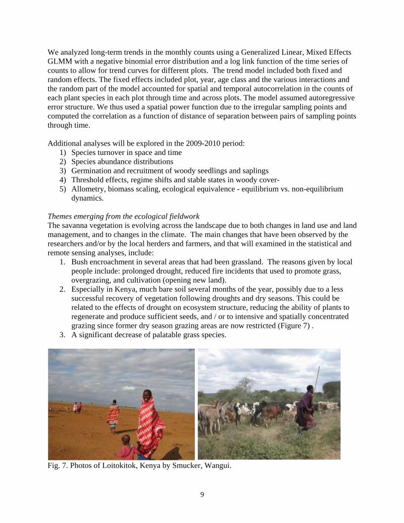
2. Especially in Kenya, much bare soil several months of the year, possibly due to a less successful recovery of vegetation following droughts and dry seasons. This could be related to the effects of drought on ecosystem structure, reducing the ability of plants to regenerate and produce sufficient seeds, and / or to intensive and spatially concentrated grazing since former dry season grazing areas are now restricted (Figure 7) .

3. A significant decrease of palatable grass species.

Fig. 7. Photos of Loitokitok, Kenya by Smucker, Wangui.

9

Socioeconomic data collection – household surveys The purpose of the household survey is to provide information on how different types of households—those with different livelihood types (pastoralism, agro-pastoralism, mostly agriculture) and of different resource levels – are being and will be affected by climate change, and how their livelihood and food security situation, land use decisions and drought coping strategies are being affected. The surveys were preceded by a wealth ranking and other exercises which had produced household lists by wealth category, and had introduced the survey team (led by Karanja) and research topic. To execute the surveys well, a Maasai woman (Sumare) interviewed the women of the households and aided in translation (from Maa to English and vice-versa). With the assistance of a key village person, each of household has been/ will be identified and visited for interview. In Loitokitok District, Kenya, three villages were chosen in which to conduct the quantitative research to overlap with the ecological and qualitative field research, and to provide a variety of livelihood types (Table 1 and Figure. 8). Each village is relatively small, comprising between 30-100 bomas (households or extended families living together). The villages are not official administrative units in Kenya, but rather informal geographical units with which people are familiar. Village Group Ranch Predominant

Livelihood Activities

Total number of wealth ranked households

Household interviewed to date

Remaining households yet to be interviewed

Empiron Kimana Livestock and agriculture

131 21 0

Mbirikani Mbirikani Livestock and Tourism-related Activities

106 20 1

Risa Olngulului-Lolarashi

Primarily Livestock

34 5 16

Table 1. Villages and households being surveyed in Loitokitok District, Kenya. The surveys in Loitokitok District, Kenya were started in June and July, 2008. Thirty surveys are being conducted in each of three villages: Mbirikani, Mpiron, and Lisa. By the end of July, 2008, only 15 and 4 household had been interviewed in Mpiron and Mbirikani respectively. In 2009 (from June- to date) we finished the remaining 4 households in Mpiron, plus 16 households in Mbirikani, and are attempting to conduct the survey in Risa. However, a major difficulty we are facing is that most households have moved with their livestock in search of green pastures, due to the ongoing drought. Some of the locations households have moved into include;- Kitengela, Chyulu hills, Taveta, Ukunda-Mombasa, Voi, Rombo and across the border to Tanzania (several over 50 kilometers from their homes). Consequently, we are forced to ask where they can be found, and we try to seek them. Similar plans are underway to complete the household survey in three villages in Simanjiro, Tanzania (Figure 9) but the problem of households having scattered due to the drought is being faced there, too. In the meantime, a data entry format for the questionnaire was completed and data entry is on-going.

10

Fig. 8. Location of villages where socioeconomic data is being collected in Loitokitok District, Kenya.

Terat

Kitwei A

Namalulu

Fig. 9. Location of villages where socioeconomic data is being collected in Simanjiro District, Tanzania. The household survey data will be analyzed using the IMPACT model and a variety of statistical methods. This model will be used to run baseline analysis on such issues as food security, household labor flow and seasonal nutrient production.

11

Socioeconomic data collection – qualitative field research The focus of the qualitative socioeconomic field research is to understand how pastoralist land use and livelihoods are changing in light of recent climate and vegetation changes, and other drivers of change at the community and higher levels. The village level case studies will assist with our understanding the dynamics of vulnerability and resilience through documenting trends in livelihood adaptation and the advent of new coping strategies. A cross-site, comparative case study approach is being implemented to understand changes in savanna land management through the broader lens of changing livelihoods and coping strategies, as land management is embedded in the dynamics of livelihood and coping. The fieldwork in Loitokitok District, Kenya was conducted by Smucker and Wangui in May, June and July, 2008. In each of villages, three community meetings and multiple key informant interviews were carried out. The meetings were taped and transcribed. A parallel effort is underway in Simanjiro, Tanzania by Mong’ong’o. People in two villages in Simanjiro, Kitwai A and Namalulu have been interviewed but the third village, Terat, has not been completed due to the problem of households having been significantly affected by the drought. The themes coming from the qualitative fieldwork will be explored more thoroughly when the household survey, remote sensing and other data has been analyzed. Feedback workshops will be conducted to provide the communities the results of the research and to confirm with them our interpretation of the information. Wealth Ranking Discussions. Wealth ranking forums explored local socioeconomic differentiation, how this differentiation has changed in the recent past, and which kinds of livelihood activities are seen as least and most vulnerable to climate variability. In addition, a list of potential household survey respondents were categorized into three wealth groups. Community Mapping Forums. Mapping forums explored the geography of overlapping livelihood spaces along the transects and elaborated the relationship between land management and vegetation change in local contexts. Activities included sketch mapping of livelihood spaces such as key land and water resources that participants manage/use directly (Fig. 10). The mapping exercise was followed by a discussion of environmental changes in each area and the implications for livestock management. Groups of men and women prepared separate maps. Fig. 10. Map of livelihood space and key resources created by participants in community mapping forum (Risa, Loitoktok District, Kenya)

12

Livelihoods/Coping/Land Management Timeline Discussions. Small group discussions were held to identify the primary shifts that have occurred in the following areas:

• how livelihood and coping strategies have changed over the last 25 years. People’s management of savanna landscapes is embedded in broader livelihood strategies, and may also reflect adaptation to local environmental change (e.g., changing rainfall patterns, vegetation composition, etc.). The meetings elicited narratives of change over the last 25 years as a means of elaborating the interrelationships between livelihood, land and livestock management, and environmental change in each local context. A particular concern will be to identify and explain the timing of major shifts in livelihood and management. These shifts will later be examined relative to the analysis of MODIS imagery over the same period (1982-2008).

• Meetings participants discussed how vegetation has changed over time and how peoples’ use of land/grazing and other resource use strategies have changed over time as a result (herd composition/numbers, herding strategies, fire; new land uses); incorporate questions that reflect the livelihood-vegetation connection

• Projections of future livelihood/coping options. Preliminary Findings of Socioeconomic Field Research Preliminary analyses based on qualitative data suggest a rapidly changing social geography of vulnerability to climatic variability that may be exacerbated by more frequent and more intense droughts and the broad trend toward the privatization of resources access. Among the major areas of change discussed by participants were:

• Further diversification of livelihoods • Deepening socio-economic differentiation • Changing gender divisions of labor • Changing institutional articulations • Changing dynamics of livestock mobility • Vegetation change and responses in fuelwood collection areas • Vegetation change and responses in grazing areas.

These will be briefly explained below. Further Diversification of Livelihoods. The transition toward sedentarization and diversification of livelihood strategies has progressed and taken on new forms. Each of the study villages report growing involvement in crop production (as wage laborers and farmers on rented or purchased land) and non-farm activities. The importance of agriculture emerged in discussions in each of the communities, though linkages to the agricultural economy vary within and between communities. In Kenya, those who have been allocated land that can be irrigated are generally benefiting most. Others who have not been allocated land or who are not experienced farmers tend to engage in casual labor on irrigated farms. In Tanzania, large scale farmers had been allocated large tracts of land by the government; many have recently abandoned their farms due to the increasingly insufficient rains, leaving large cleared areas on the landscape. On the whole, people tend to speak reluctantly about the benefits of agriculture and many lament the demise of pastoral mobility. Several factors have further added to the risk associated with livestock keeping. Disease was cited as a major concern. Traditional treatments are seen as ineffective while modern veterinary

13

treatment was commercialized in the 1990’s and remains out of reach for many livestock keepers. Furthermore, school attendance has increased since the advent of the 2003 “free primary” policy, which further discouraged mobility. Declining mobility and greater diversification may contribute to changing views of wildlife as an economic asset (in Kenya, not so much in Tanzania). A common development observed was providing services for mobile phones (e.g., repair, charging, etc.). A new development in diversification is the growing participation of women in non-farm activities (both as casual laborers and in micro-enterprise). In Tanzania, income accrued from the mining business has been used to change the pastoralists’ way of life, including building of modern houses, buying and owning motorcycles, vehicles, telephones and generators for electrifying their houses. Participants from all communities in Kenya noted an increase in socioeconomic inequality that has accompanied livelihood diversification and, with the exception of Risa, land subdivision. In developing criteria for wealth ranking in each community, a tension was observed between the cultural prestige associated with livestock (particularly cattle) ownership and the realities of a more diversified livelihood system in which non-farm sources of income may be a more important indicator of household well-being. It should be noted that in discussing wealth or general well-being, respondents rarely took a narrow economic view and tended to frame the wealth categories relative to broader concerns for social relations and community standing. In Tanzania, the social network and sharing of resources between wealth categories is breaking down as pastoralism evolves. The rich tend to keep large herds of cattle as a strategy to accumulate wealth. Traditionally when the herds get too big and unmanageable by an individual

they split them into smaller units and loan them to either the moderately rich people or the poor to take care of them. In payment the keeper drinks the milk and keeps some of the heifers born in the new place. The poor benefit and are able to positively shift their position on the wealth spectrum to a relatively better wealth category. The system is disintegrating as Maasai traditional institutions are no longer tenable. Today the wealthy sell a few bulls to have money to hire someone to care for their other animals. The rich are also diversifying into business, especially through selling of livestock and investing in lucrative enterprises buying and minerals. Water and grazing are being privatized, especially during droughts.

Fig 11. Mong’ong’o and herder constructing the village timeline in Kitwai A, Tanzania. Photo by Olson. The criteria established for wealth categories varied among the villages. In Empiron, for example, lack of formal landholding was seen as an important indicator of poverty as was the

14

passing up of free public education to send children to academies. However, cattle remain important, suggesting that pasture is still available in the aftermath of subdivision to those who can use market and social relations to access them. In pre-subdivision Risa, cattle and wives remain central to peoples’ thinking about wealth given the enduring importance of the labor of wives and children to livestock keeping. Even in Risa, access to or ownership of more than thirty acres of land for cultivation is seen as an important indicator of wealth. In contrast, cattle and other animals, and wives and children are the only indicators of wealth in Kitwai A in Tanzania, where land is basically communal and not lacking. The wealthiest groups in Tanzania were defined as having at least 500 cattle and many other animals, and 6 or more wives. Wealth Class Empiron Mbirikani Risa Wealthy • > 5 acres, owned

• > 100 cattle • has employees • take children to

‘academies’

• > 100 cattle • salaried

employment

• > 100 cattle • > 30 acres • > six wives • Educated children

Poor • Landless; • No livestock • Casual worker

• < 10 cattle; • No employment

• Less than 10 cattle; • No wife or children

Table 2. Wealth Ranking Criteria Identified by Participants in Kenya. Using their own criteria, each village categorized all households in the community into one of the wealth categories. In Kenya, the largest wealth category pre-subdivision Risa was the wealthy group. In Mbirikani, on the precipice of subdivision, the groups were evenly divided. In post-subdivision Empiron, the wealthy group was by far the smallest. Empiron Mbirikani Risa Wealthy 18 (12%) 39 (37%) 14 (44%) Middle 68 (45%) 36 (34%) 7 (22%) Poor 64 (43%) 30 (39%) 11 (34%) Table 3. Distribution of Households by Wealth Rank in Loikotikok, Kenya. This differentiation has implications with how people manage climatic variability. In all sites, people recognized that the poor were most vulnerable to losing or being forced to liquidate productive resources during drought, and that wealthy people were less immediately impacted by drought, both because they maintained the ability to move livestock through pasture rental and because they could rely on non-farm activities for income during drought periods:

There is a big difference between the rich and the poor in terms of survival during bad times. The rich are able to save more of their livestock as they have the resources and money to rent extra land for their livestock to feed on. The rich are also better placed during bad droughts as besides keeping livestock they also have got some other extra sources of income to rely on, like small businesses and farming. (Empiron male)

Discussions highlighted the difficulties of building and maintaining viable herds in light of perceived declining and less predictable rainfall:

15

In the past it was easy to keep livestock. Nowadays it is hard to raise livestock due to the fact that the rains have become shorter and unpredictable. In the past there was adequate rainfall to let the grass to grow, there were few and short drought periods. Nowadays the rains are shorter, and the droughts are more frequent many things depend on rain like livestock keeping and crop farming. An example is a man who had around 2,000 cows but is now being given food rations by the government as the cattle have no value when there is a drought. But if there was rain, the 2,000 heads of cattle would have helped the man and his family, so everything is highly depended on the availability of the rains. (Risa male)

Goats and sheep tend to survive better than cattle with the reduced rainfall and loss of grass, so herds in Tanzania are tending to have a higher ratio of small stock to cattle. However, people still need to keep cattle. Cattle are more highly valued; they are needed for getting wives (dowry), the wives need the milking cows, and the price of cattle is higher. Nevertheless, herd composition is significantly changing. In Kenya, herders are experimenting with drought resistant goat and sheep from Somalia that unfortunately eat down to the grass roots, leaving the landscape less able to recover when rains return. Changing Gender Divisions of Labor Women’s contributions to new livelihood activities have evolved dramatically. The free primary education policy, instituted in 2003 in Kenya, resulted in a massive influx of school age children into local schools and consequently created a shortage of labor for herding in many bomas. Women seem to have filled this gap by and large, and now engage in both local and long distance movements to dry season grazing areas, particularly in Risa. This has created a tension between women’s livestock activities far from the boma and traditional responsibilities in the boma. Women’s ole in managing changing grazing environments will likely increase, but their perspective on vegetation is relatively short-term given their recent entry into herding. Women also discussed small business and trading activities as particularly important during drought. Longer-term development strategies, such as the formation of local women’s CBOs to develop saving schemes, are put on hold during these times. Other themes that came out of the discussions include changing livestock mobility and grazing patterns due to land tenure, drought and social factors, changing vegetation structure and forage quality, and the role of institutions. Changing Gender Roles Master’s Thesis The thesis research of a UDSM Master’s student (Euster Kibona) was conducted under the EACLIPSE umbrella. It examined climate variability / change adaptation strategies and their impacts on gender roles in Simanjiro District. Quantitative data was collected with questionnaires and qualitative data was collected using Participatory Rural Appraisal tools. Agro-pastoral communities living in harsh conditions of climate have been able to cope with periodic drought and other climatic difficulties. They are used to handling adversity and risk, but climate change is presenting a burden that is likely to go beyond their historical experience. The study found that as climate change unfolds, communities have been responding including

16

changing their livestock migration patterns. This has resulted in shifts in gender roles. Men are finding themselves away from home for long periods of time and their previous tasks nearer the home are now being performed by women. This is in addition to the numerous domestic chores already performed by women. In this transitional stage, some gender roles have been disjointed. While the women remain responsible for feeding the household, they do not have regular access to cash to purchase supplemental foods. Cash proceeds obtained from the sale of livestock products such as milk are controlled by men. Thus for cash needs, most women have to depend upon their husbands or male relatives. Further, while the introduction of agriculture provides alternative foods for the household, it has tended to be an additional work activity for women (simply because that is what happens in agricultural communities) and has thus increased women's work loads. Impact of Land Use /Land Cover Changes on Resource Management Master’s Thesis A second Master’s thesis was conducted under the EACLIPSE umbrella at UDSM. Jacqueline Senyagwa examined changing land use/ land cover (LULCC) in the Namalulu and Naberere area Simanjiro, and how that has affected natural resource management. The research employed qualitative and quantitative approaches in data collection. The type of data collected ranged from key informant interviews, a household survey, remote sensing (Landsat TM) analysis, and collection of secondary data. Water and tree resources in forests were founds to be the resources most affected by LULCC, especially the expansion of agriculture. In the future, however, agriculture is not expected to play as large a role due to the failure of many especially large scale farms due to low rainfall, and different patterns are expected as summarized in Table 4. . Drivers affecting future land use Frequency Percent Clearing of forests to open new farms 21 30 Charcoal making 10 14 Tribalism: Maasai offered large chunks of land 1 1 Not enforcing laws 7 10 Poor leadership 5 7 Climate change 5 7 Unsystematic selling of land 5 7 Population increase 5 7 Soil degradation 1 1 Increase in agriculture subsidies 6 9 Agriculture given priority nationally 2 3 Opening of mining sites 1 1 Total 69 100

Table 4. Drivers of LULCC expected to affect natural resources in the future (survey results).

17

Remote sensing analysis The main purpose of the analysis of remotely sensed data is to identify trends over space and time in changing vegetative patterns, and explain these patterns in terms of weather/ climate and human land use / land management. The project researchers Qi and Chuan are analyzing the GIMMS dataset (bi-monthly, 1982 to 2008) and more recent MODIS time series images to identify changes in amounts and seasonality of the vegetation (NDVI) using the TIMESAT model. East Africa is a very complex region to analyze changes in seasonality because it straddles the equator and has areas of bi-modal rainfall (with different areas having the long and the short rainy season), and areas of uni-modal rainfall but where the one rainy season occurs at

different times of the year. TIMESAT does not handle this very well. We have been able to identify trends in the start and duration of the growing seasons. Figure 12 illustrates one result of the on-going analysis, of changes in the “large integral” (total amount of growth of vegetation during the rainy season). It shows that generally Northeastern Kenya and southern Sudan are trending towards more vegetative growth, whereas central Tanzania and areas in Kenya and Uganda are experiencing a decline in vegetative growth. This is fairly consistent with the results of our regional climate and crop-climate modeling, in which the northern part of our domain is / will experience increasing rainfall but elsewhere yields will decline due to the warming temperatures and no increase or a decreased in precipitation. Fig. 12. Change in vegetation amounts (large integral in TIMESAT analysis) between 1984 and 2005 (blue is increase, red is decrease).

The changes in seasons and vegetation amounts will be compared to climate data that we have to identify the relationship between them, and to identify areas where human activity may have an important role affecting the vegetation. This approach has been develop using data from China, where afforestation, deforestation and urbanization have had large impacts on vegetation. In East Africa, we anticipate that areas of recent increases in land use intensity, such as in southern Kenya where savanna land has been sub-divided and become intensely grazed or cultivated, may become apparent in GIMMS data. However, Said and Mwansasu are also conducting higher resolution imagery analysis of the sites where we are collecting field data. This higher resolution imagery (Landsat TM, QuickBird) will be used to identify whether vegetation changes that the field ecologists and the local herders and farmers described, including bush encroachment in some areas and .significant loss of vegetative cover in others is visible, and what of it can be linked to weather/ climate changes.

18

Simulations of climate/ vegetation and surface water The objective of the coupled climate/ vegetation and surface water modeling is to identify the relationship between climate and vegetation trends, and to simulate the effect of climate change on vegetation productivity and on the availability of surface water. This analysis is being informed by the remote sensing analysis. Initial modeling has been done by Alagarswamy at the 18 km2 resolution (which will be done for the entire domain), but within the boxes the modeling will be done at a 6 km2 resolution. We are using the ecosystem Century Soil Organic Matter Model (v 4.5) to simulate grass biomass and soil carbon (Metherell et al. 1993). We will later simulate other vegetation types, and crops similar to what we did in our earlier CLIP project. Century model requires weather data minimum and maximum air temperature and precipitation at monthly intervals, and soil physical attributes (texture, bulk density) as input data. We used temporal weather data from the WorldCLIM data set (Hijmans et al., 2005) for current climate representing the period 1951-2002. Daily maximum and minimum air temperatures and precipitation amounts were generated from monthly climate normals for each grid synthetically using the MarkSim weather generator (Jones and Thornton, 2000). Additional details on the methods used in climate data development are given in Thornton et al. (2009). Thirty replicates of monthly weather data of different weather years were generated from climatological base line current climate normals from WorldCLIM. All agriculturally suitable soil types in the study area were defined on the basis of the FAO (1978) soil unit ratings. Soil textural and other input data for those soil types were taken from the International Soils Reference and Information Centre’s World Inventory of Soil Emission Potentials (WISE) database (Batjes and Bridges, 1994), as modified and reformatted by Gijsman et al. (2007). As initial soil carbon values for the study sites were not available, Century model was run for a longer time frame (about 2000 years) to simulate initial soil carbon for the current climate period using stochastic meteorological data generated using monthly weather data derived from WorldClim. Fig. 13 presents an example of calibrated Century model result for initial soil carbon in a typical soil in the study site. Longer time frame initial runs were needed to reach equilibrium soil carbon contents. Subsequent to longer equilibrium period, simulation results indicate sharp decline in soil carbon content which represented normal soil carbon losses in a cultivated land representing enhanced decomposition of organic matter as well due to a reduction in crop residue incorporation to the soils (Donigian et al., 1994, Mikhailova et al., 2000).

19

Fig. 13. Simulating equilibrium soil organic matter content in a selected study site pixel by the Century model.

Figure 14 shows simulated grass production in both EACLIPSE study sites for the curren, period (representing 1970-2002) to serve as base line for comparing the impact of future climate change on grass production. Grass yield in the southern study site ranged from 125 to 400 g/m2 with a mean of 266 (SD 42) while in the northern study site grass yield varied from 75 to 400 g/m2 with a mean of 230 g/m2 (SD 86 ). The southern study site pixels were more productive as simulated grass yield were greater than 225 g/m2 in 85% of the pixels (out of total 223 pixels). The northern study site was comparatively less productive in terms of grass yield as only 50% of the pixels (out of total 123 pixels) recorded grass production greater than 225 g/m2. The coefficient of variation for the southern site was 15% and for the northern site was 37%, indicating greater dispersion of grass yields with in the northern study site. Substantial spatial heterogeneity existed in grass yield in both the study sites. Simulated grass yields were within the range of reported (220 – 340 g/m2) in Nairobi National park and in Masai Mara game by Owaga 1980, Desmuk 1986, Bouton et al. 1987 and Kinyamario, and Imbamba, 1992.

20

Fig.14 (left). Grass biomass (g/m2) simulated for Fig. 15 (right). Simulated total soil the current period by CENTURY model in study carbon (g/m2) in 20 cm soil depth sites. for current period by CENTURY model in study sites. Figure 15 shows simulated total carbon in the soil (top 20 cm depth) in both study sites for the current period (representing 1970-2002) to serve as base line for comparing the impact of future climate change on soil carbon losses. Soil carbon in the southern study site ranged from 1370 to 5140 g/m2 with a mean of 3420 (SD 640) while in the northern study site soil carbon ranged from 950 to 5900 g/m2 with a mean of 2730 g/m2 (SD 1523). The coefficient of variation for the southern site was 19% and for the northern site was 56%, indicating the greater dispersion of soil carbon stock with in the northern study site. Simulated soil carbon content was comparable to observed 6250 g/m2 for Nairobi national park (Ojima et al.1996). The base line simulated grass productivity and soil carbon data will be used to assess climate change effects on savanna productivity, its ability to support live stock and pastoral activities in the future. The base line grass productivity data also will be used to link NPP/ NDVI estimated from remote sensing products from MODIS and to field level measurements at study sites. The Century biomass results are being validated using MODIS data. Figure 16 illustrates the annual biomass (net primary productivity) from an analysis of MODIS images for year 2000 on the left compared against the grass biomass yield pattern produced by the Century Model on the right in our northern study site.

21

. Fig. 16. Comparison of MODIS derived net primary productivity on the left, and grass biomass Century model results on the right in our northern site. In addition, the surface water model SWAT is being prepared in order to simulate the effect of climate change on surface water availability for livestock and people. The remote sensing analysis and Century simulations of grass biomass productivity will inform livestock productivity modeling (using RUMINANT), which will then inform the household survey modeling and analysis to identify the impact of climate change on household food security and income. Climate data analysis and simulations Perhaps this report should have started with the results of the analyses of historical climate data, and simulations of future climates. Historical climate is being examined using various datasets including meteorological station data where available, spatially explicit East Anglia’s Climatic Research Unit (CRU) and ERA40 data. The basic questions being asked are, What if any are the trends in temperature and precipitation? Are the frequency and severity of droughts changing? To address these questions, a variety of time series statistical approaches have been tested on data for precipitation and temperature. Historical Precipitation Trends We used the Standardized Precipitation Index (SPI) to compare the cumulative precipitation over selected time scales (6, 12, 24, 36 months, etc.) to the historic record. These values are then

22

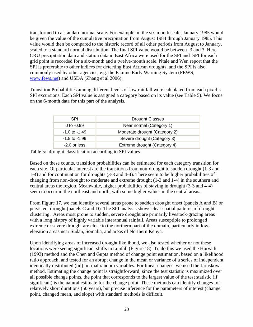
transformed to a standard normal scale. For example on the six-month scale, January 1985 would be given the value of the cumulative precipitation from August 1984 through January 1985. This value would then be compared to the historic record of all other periods from August to January, scaled to a standard normal distribution. The final SPI value would be between -3 and 3. Here CRU precipitation data and station data in East Africa were used for the SPI and SPI for each grid point is recorded for a six-month and a twelve-month scale. Ntale and Wen report that the SPI is preferable to other indices for detecting East African droughts, and the SPI is also commonly used by other agencies, e.g. the Famine Early Warning System (FEWS; www.fews.net) and USDA (Zhang et al 2006). Transition Probabilities among different levels of low rainfall were calculated from each pixel’s SPI excursions. Each SPI value is assigned a category based on its value (see Table 5). We focus on the 6-month data for this part of the analysis.

SPI Drought Classes 0 to -0.99 Near normal (Category 1)

-1.0 to -1.49 Moderate drought (Category 2) -1.5 to -1.99 Severe drought (Category 3) -2.0 or less Extreme drought (Category 4)

Table 5: drought classification according to SPI values Based on these counts, transition probabilities can be estimated for each category transition for each site. Of particular interest are the transitions from non-drought to sudden drought (1-3 and 1-4) and for continuation for droughts (3-3 and 4-4). There seem to be higher probabilities of changing from non-drought to moderate and extreme drought (1-3 and 1-4) in the southern and central areas the region. Meanwhile, higher probabilities of staying in drought (3-3 and 4-4) seem to occur in the northeast and north, with some higher values in the central areas. From Figure 17, we can identify several areas prone to sudden drought onset (panels A and B) or persistent drought (panels C and D). The SPI analysis shows clear spatial patterns of drought clustering. Areas most prone to sudden, severe drought are primarily livestock-grazing areas with a long history of highly variable interannual rainfall. Areas susceptible to prolonged extreme or severe drought are close to the northern part of the domain, particularly in low-elevation areas near Sudan, Somalia, and areas of Northern Kenya. Upon identifying areas of increased drought likelihood, we also tested whether or not these locations were seeing significant shifts in rainfall (Figure 18). To do this we used the Horvath (1993) method and the Chen and Gupta method of change point estimation, based on a likelihood ratio approach, and tested for an abrupt change in the mean or variance of a series of independent identically distributed (iid) normal random variables. For linear changes, we used the Jaruskova method. Estimating the change point is straightforward; since the test statistic is maximized over all possible change points, the point that corresponds to the largest value of the test statistic (if significant) is the natural estimate for the change point. These methods can identify changes for relatively short durations (50 years), but precise inference for the parameters of interest (change point, changed mean, and slope) with standard methods is difficult.

23

ig. 17. Spatial distribution of transition probabilities for: (A) normal conditions to severe me

Fdrought; (B) normal conditions to extreme drought; (C) severe drought continuing; (D) extredrought continuing.

24

Time of Change

No Cha

nge

&

1950

-1960

&

1960

-1970

&

1970

-1980

&

1980

-1990

&

1990

-2000

&

2000

-2002

Fig. 18. Statistically significant changes in rainfall based on CRU change point analysis. The precipitation for both the CRU and the ERA40 shows little change in most sites (and disagree for much of the domain!), but the changes that do occur are decreases in means (with a couple sites showing changes in variance). These decreases do not seem to happen within a similar time period. This would suggest local changes as opposed to regional changes. However, the variability of the change point estimates is large, so the exact time of change is difficult to determine. The areas that do show rainfall change are concentrated in Northern Kenya, an area that may already be exhibiting increased NDVI associated with increased rainfall. Much of the changes occur around the climate shifts associated with the 1970s (Seidel and Lanzante 2004), and is likely the result of complex changes in flow from the Indian Ocean. Examples of change point detection for individual stations witnessing precipitation declines are shown in Figure 19.

Fig. 19. Examples of abrupt changes in rainfall detected by change-point analysis of meteorological station data (Iringa and Pemba, Tanzania). These results are written up in a draft for publication, anticipated for completion in October. Although these trends show relatively few areas of changing rainfall, part of the lack of signal may derive from severe paucity of data. CRU and ERA40 data are fundamentally derived from a

25

box model driven by station and radiosonde data; station data in this part of the world is notoriously sparse. Hence, the signals of change detected from such modeled data may not capture the extreme variations and numerous microclimates in this extremely varied terrain. White the detection of change using these methods is robust, the point of detection can sometimes be complicated by high variability; this variability is demonstrated in the examples of Figure 22. One additional interesting point is worth pointing out. Although most GCMs are not yet run at grid spacings suitable for making regional predictions with any skill, most of the projections of elevated greenhouse gas effects include increased precipitation in East Africa, particularly in the semiarid regions of Kenya, Sudan, and Uganda. If the processes behind these wettening areas in Northern Kenya are associated with increased Hadley cell convection in the ITCZ, then these shifts may mark some sort of early detection of greenhouse gas effects in East Africa. Fig. 20: Max Temp: Change point estimate Fig. 21: Min Temp: Change point estimate

Time of Change

No Cha

nge

&

1950

-1960

&

1960

-1970

&

1970

-1980

&

1980

-1990

&

1990

-2000

&

2000

-2002

26

Historical Temperature Trends Change point detection was also applied to the CRU temperature data and the tests show widespread increases (Figures 20 & 21). Again, it is hard to say whether these changes occurred at about the same time or not. However, the fact that so many sites had significant changes presents strong evidence that temperatures have increased in this region between 1950 and 2000. The entire domain shows warming, albeit with the change point occurring at various dates and not as consistent with any ocean or global pattern. Following Christy et al. (2009), who have pointed out the importance of treating Tmin and Tmax separately, we identify once consistent large scale pattern between the trends: both regions show the interior warming earlier than the coastal regions (Fig. 22). The reasons behind this lag are uncertain, but may be due to complex moisture processes that also influence temperature ranges. Continued simulations of climate shifts due to both GHG changes and LCLUC suggest that LCLUC along the coasts may contribute more to the coastal warming pattern, particularly since such land cover change did not begin in earnest until the adoption of more open land use policies and market liberalization in the 1980s.

Figure 22. Examples of temperature increases (meteorological station data, Mtwara, Moshi and Morogoro, Tanzania) Conclusion Year 2 of the EACLIPSE project has seen the large team active in the field and conducting innovative analyses and modelling of large remote sensing, climate and other databases in an effort to better identify and understand the impact of climate and other drivers of change on savannah vegetation, animals and people. New primary data being collected in the field is permitting a link to be established between the evolving socioeconomic and ecological systems, and climate, but it is also producing unexpected findings. Although changing land use and land management in the context of rapidly evolving agro-pastoral system is clearly having a direct effect on savannah vegetation, there are significant changes in vegetation composition and biomass productivity that will need to be examined using time series remote sensing data and the coupled climate/ vegetation and water modelling system. The current prolonged drought is affecting our ability to complete the field data collection, since plant species counts will need to wait until the rains come and plants recover, and since people have scattered across a wide area to seek water and forage for their livestock and are not available for interviews.

27

References Bouton, T.W., L.L. Tieszen, S.K. Imbambal. 1987. Biomass dynamics of grassland vegetation in

Kenya. African Journal of Ecology 26: 89-101.

Batjes, N.H., E.M. Bridges, 1994. Potential emissions of radiatively active trace gases from soil to atmosphere with special reference to methane: development of global database (WISE). J Geo. Phy. Res., 99(D8) 16:479-489.

Chen, J. & Gupta, A. K. (1997) Testing and Locating Variance Changepoints With Application to Stock Prices. J. Am. Stat. Assoc. 92, 739-747.

Desmukh, I. 1986. Primary production of a grassland in Nairobi National Park. J Appl. Ecol., 23:115-123.

FAO (Food and Agricultural Organization of the United Nations), 1978. Report on the AgroEcological Zones Project, Volume 1. Methodology and Results for Africa, UNESCO, Paris and FAO Rome.

Gijsman, A.J., P.K. Thornton, G. Hoogenboom. 2007. Using WISE database to parameterize soil inputs for crop simulation models. Computers and Electronics in Agriculture 56: 85-100.

Hijmans, R.J., S.E. Cameron, J.L. Para, P.G. Jones, A. Jarvis. 2005. Very high resolution interpolated climate surfaces for global land areas. Int. J. Climatology 25: 1965-1978.

Horváth, L. (1993). The maximum likelihood method for testing changes in the parameters of normal observations. Ann. Statist. 21, 671-680.

Jaruková, D. (1998). Testing appearance of linear trend. J. Stat. Plan. Inf. 70, 263-276.

Jones, P.G., and P.K.Thornton, 2000. MarkSim. Software to generate daily weather data for Latin America and Africa. Agron. J., 93:445-453.

Kinyamario, J.I., and S.K. Imbamba, 1992. Savanna at Nairobi National Park, Nairobi. In: Long, S.P., M.B. Jones, and M.J. Roberts. (Eds)., Primary Productivity of Grass Ecosystems, Chapter 2. Chapman and Hall, London.

Metherell, A. K., L.A. Harding, C.V. Cole, W.J. Parton. 1993. CENTURY Soil Organic Matter Model Environment. Technical Documentation, Agroecosystem Version 4.0 Great Plains System Research Unit, Technical Report No. 4. USDA-ARS, Fort Collins, CO.

Owaga, M.L.A. 1980. Primary productivity and herbage utilization by herbivores in Kaputei plains, Kenya. African J Ecol., 18:1-5.

Ojima, D.S., W.J. Parton, M.B. Coughenour, J.M.O. Scurlock, T.B. Kirchner, T.G.F. Kittel, D.O. Hall, D.S. Schimel, E.G. Moya, T.G. Gilmanov, T.R. Seastedt, A. Kamnalput, J.L. Kinyamario, S.P. Long, J.C. Menaut, O.E. Sala, R.J. Scholes, and J.A. van Veen. 1995. In: Breymeyer, A.I., D.O.Hall., J.M. Melillo, and G.I. Agren. (Eds)., Global Change: Effects on Coniferous Forests and Grasslands. Chapter 12,John Wiley & Sons, Chichester, New York, Brisbane, Toronto, Singapore.

Seidel D. J., J. R. Lanzante (2004), An assessment of three alternatives to linear trends for characterizing global atmospheric temperature changes, J. Geophys. Res., 109, D14108, doi:10.1029/2003JD004414.

28

Thornton, P.K., P.G. Jones, G Alagarswamy, J Andresen. 2009. Spatial variation of crop yield response to climate change in East Africa. Global Env. Change 19, 1: 54-65.

Zhang, P., B. T. Anderson, and R. Myneni (2006), Monitoring 2005 Corn Belt Yields From Space, Eos Trans. AGU, 87(15), doi:10.1029/2006EO150003.

29