Exploiting noise in array CGH data to improvedetection of DNA copy number changeJing Hu, Jian-Bo Gao*, Yinhe Cao1, Erwin Bottinger2 and Weijia Zhang2,*

Department of Electrical and Computer Engineering, University of Florida, Gainesville, FL 32611, 1Biosieve,1026 Springfield Drive, Campbell, CA 95008 and 2Department of Medicine, Mount Sinai School of Medicine,One Gustave L. Levy Place, New York, NY 10029, USA

Received April 14, 2006; Revised September 20, 2006; Accepted September 21, 2006

ABSTRACT

Developing effective methods for analyzing array-CGH data to detect chromosomal aberrations isvery important for the diagnosis of pathogenesisof cancer and other diseases. Current analysismethods, being largely based on smoothing and/orsegmentation, are not quite capable of detectingboth the aberration regions and the boundary breakpoints very accurately. Furthermore, when evaluat-ing the accuracy of an algorithm for analyzing array-CGH data, it is commonly assumed that noise inthe data follows normal distribution. A fundamentalquestion is whether noise in array-CGH is indeedGaussian, and if not, can one exploit the character-istics of noise to develop novel analysis methodsthat are capable of detecting accurately the aberra-tion regions as well as the boundary break pointssimultaneously? By analyzing bacterial artificialchromosomes (BACs) arrays with an average 1 Mbresolution, 19 k oligo arrays with the average probespacing <100 kb and 385 k oligo arrays with theaverage probe spacing of about 6 kb, we show thatwhen there are aberrations, noise in all three typesof arrays is highly non-Gaussian and possesseslong-range spatial correlations, and that such noiseleads to worse performance of existing methodsfor detecting aberrations in array-CGH than theGaussian noise case. We further develop a novelmethod, which has optimally exploited the charac-ter of the noise, and is capable of identifying bothaberration regions as well as the boundary breakpoints very accurately. Finally, we propose a newconcept, posteriori signal-to-noise ratio (p � SNR),to assign certain confidence level to an aberrationregion and boundaries detected.

INTRODUCTION

Amplification or deletion of chromosomal segments can leadto abnormal mRNA transcript levels and result in the mal-functioning of cellular processes. Locating chromosomalaberrations in genomic DNA samples is an important stepin understanding the pathogenesis of many diseases, mostnotably cancers. Microarray-based comparative genomichybridization (array CGH) is a powerful technique for mea-suring such changes (1–5). To realize the promise of thearray CGH technique, it is very important to develop effec-tive methods to identify aberration regions from array CGHdata. Existing analysis methods (6–23) can be roughly classi-fied into two categories: smoothing-based (6–9) andsegmentation-based (10–19). The latter approaches explicitlymodel the observed array data as a series of segments, withunknown boundaries and unknown heights estimated fromthe data by employing certain optimization criterion. Whilethe boundary points thus identified are reliable, the aberrationregions identified may be less so, in the sense that some ofthem may be false positives. Smoothing-based approachesassume that true signals in a specific region, aberration ornon-aberration, are smoother than any kind of noise superim-posed on the signals. Therefore, they attempt to reduce noiseby comparing individual data points to their adjacent onesand modifying them. While such methods can reduce thenumber of false aberration regions identified, the boundarypoints detected are usually less accurate than segmentation-based methods. It would be very desirable to develop newmethods for analyzing array CGH data, with both the meritsof smoothing and segmentation based approaches. Such agoal may not be fully accomplished by just incorporatingmean or median smoothing to a segmentation-based method.

The term ‘noise’ is often used in biology to describeexperimental measurement imprecision. In particular, whenevaluating the accuracy of an algorithm for detecting aberra-tions, it is commonly assumed that noise in the data followsnormal distribution. However, this important assumptionhas not been verified/falsified based on the analysis of

*To whom correspondence should be addressed. Tel: +1 2122412883; Fax: +1 2128492643; Email: weijia.zhang@mssm.edu*Correspondence may also be addressed to Jian-Bo Gao. Tel: +1 3523920918; Fax: +1 3523920044; Email: gao@ece.ufl.edu

� 2007 The Author(s).This is an Open Access article distributed under the terms of the Creative Commons Attribution Non-Commercial License (http://creativecommons.org/licenses/by-nc/2.0/uk/) which permits unrestricted non-commercial use, distribution, and reproduction in any medium, provided the original work is properly cited.

Nucleic Acids Research, 2007, Vol. 35, No. 5 e35doi:10.1093/nar/gkl730

experimental data. More importantly, one has to ask whetherthe performance of an algorithm depends on the character ofthe noise, and if yes, can one exploit the characteristics ofnoise to improve detection of aberrations?

To address the above questions, in this work, we treat anydeviations from mean values as noise. Therefore, our noiseessentially represents the array CGH measurements them-selves, encompassing both global measurement imprecisionand localized underlying biological alterations. Based onthe analysis of bacterial artificial chromosomes (BACs)arrays with an average 1 Mb resolution (2), 19 k oligo arrayswith the average probe spacing <100 kb (24) and 385 k oligoarrays with the average probe spacing of about 6 kb (http://www.nimblegen.com/products/cgh/), we show that whenthere are aberrations, noise in all three types of arrays ishighly non-Gaussian and possesses long-range spatial corre-lations. We also show that such noise indeed leads to worseperformance of existing methods for detecting aberrations inarray-CGH than the Gaussian noise case. Fortunately, suchnoise can be exploited to devise a novel algorithm foranalyzing array-CGH, which is capable of identifying bothaberration regions as well as the boundary break pointsvery accurately. We also address the fundamental questionof how to assign certain confidence level to an aberrationregion and boundaries detected, by proposing a new concept,posteriori signal-to-noise ratio (p � SNR).

CHARACTERIZATION OF NOISE IN ARRAY CGH

In this section, we carry out distributional analysis as well asspatial correlation analysis of array-CGH noise, and assessthe effect of such noise on the performance of published algo-rithms for detecting aberrations from array-CGH data. Below,we first describe data.

Data

In this paper, we analyze data of three resolutions, BAC array(2), 19 k oligo array (24) and 385 k oligo array (http://www.nimblegen.com/products/cgh/). The BAC array (2) hasan average 1 Mb resolution. It is from Stanford University,which can be freely downloaded from http://www.nature.com/ng/journal/v29/n3/suppinfo/ng754_S1.html. It consistedof 15 human cell lines with known karyotypes (12 fibroblastcell lines, 2 chorionic villus cell lines and 1 lymphoblast cellline) from the NIGMS Human Genetics Cell Repository.Each cell line had been hybridized with an array CGH of2276 BACs, spotted in triplicate. The variable used foranalysis was the normalized average of the log base 2 testover reference ratio, as processed by the original authors. Ineach cell line, there were either one or two aberrations.Among the 15 cell lines, 6 had aberrations that covered anentire chromosome. Note that some of these datasets wererecently used by Olshen and Vankatraman (12) to evaluatethe effectiveness of their algorithm for detecting aberrationsfrom the data. For convenience, the names of the 15 celllines are listed in the first column of Table 1.

The 19 k oligo array data (24) are from Harvard MedicalSchool. It has an average probe spacing of <100 kb. The com-plete OligoLibrary consists of 18 861 oligos representing18 664 LEADSTM clusters and 197 positive controls. There

are four datasets for lymphoma tumors that developed inATM deficient mice (24).

The 385 k oligo array data http://www.nimblegen.com/products/cgh/ has a median probe spacing of 6 000 bpthrough genic and intergenic regions. There are two datasetsfor the 385 k oligo array data. One is the normal female ver-sus male case, where polymorphisms are observed by ourmethod (to be described later) in chromosomes 1, 4 and 5.Another is the tumor case, where chromosome 8 has the long-est aberration length (�2000), while chromosomes 10 and19–22 do not have detectable aberrations at all (see Figure1). Note that if we downsample the data to a resolution com-parable to the BAC array data (2), then the longest aberrationregion in chromosome 8 only has less than 20 points. There-fore, the 385 k oligo array data http://www.nimblegen.com/products/cgh/ has the smallest aberration regions.

Distributional analysis of array CGH noise

When carrying out distributional analysis, an important issueto consider is the size of the sample points. For the 385 koligo array data http://www.nimblegen.com/products/cgh/,we have considered noise for each chromosome in two scena-rios, corresponding to that aberration and non-aberrationregions (i) are considered together and (ii) are consideredseparately. The results are similar for both scenarios. Forthe BAC array data (2) and the 19 k oligo array data (24),we have also considered two cases, (i) each chromosome isconsidered separately and (ii) all the chromosomes arecombined together. While the distribution for all the chro-mosomes combined is not the same as that for individualchromosomes, the qualitative feature of deviation fromGaussian distributions is similar for both cases. Comparisonsof these different scenarios suggest that the non-Gaussiandistributions discussed below may not be due to summationof multiple Gaussian distributions with different variance,corresponding to the euploid and copy-number-variant partsof the chromosome. In the main text here, we present resultsfor the first scenario for all three types of data. Readers inter-ested in knowing more details about the second scenario arereferred to Supplementary Figures 1–3.

Table 1. p � SNR and Hurst parameter for noise of the 15 BAC array data (2)

Cell line/chromosome(s) p � SNR H

GM01750/9/14 3.555/5.905 0.743GM01524/6 5.308 0.739GM01535/5/12 4.032/12.170 0.688GM03134/8 2.829 0.619GM03563/3/9 3.910/11.019 0.715GM05296/10/11 5.793/3.741 0.666GM07081/7 3.193 0.664GM13031/17 5.172 0.667GM13330/1/4 3.982/7.947 0.663GM00143/18 4.429 0.741GM02948/13 3.960 0.718GM03576/2/21 5.080/5.473 0.770GM04435/16/21 4.337/4.266 0.707GM07408/20 5.774 0.712GM10315/22 5.277 0.728

When there are two aberration regions, p � SNR is defined for both regions.

e35 Nucleic Acids Research, 2007, Vol. 35, No. 5 PAGE 2 OF 10

To simplify analysis, we have simply formed histograms.This is justified by noticing that the number of sample pointsis large in all the datasets. The distributions for the noise intwo of the 15 BAC array data (cell line GM05296 andGM04435) are shown in Figure 2a and b. We observe thatthe distribution deviates from the Gaussian distributionconsiderably. In fact, these are typical results for the BACarray data (2). The distribution of noise in the 19 k oligoarray data (24) is even more non-Gaussian, as shown inFigure 2c and d, which are typical among the four datasets.Since the 19 k oligo array data (24) has wider aberrationregions, we suspect that the deviation from Gaussian distribu-tion is positively correlated with the length of aberrationregions. This hypothesis seems to be supported by analysisof the 385 k oligo array data http://www.nimblegen.com/products/cgh/. In Figure 2e–h we have shown the distribu-tions for noise in chromosomes 8 and 9 of both the normaland tumor cases, where Figure 2e and g are for the normalcase, while Figure 2f and h are for the tumor case. Notethat distributions for noise in other chromosomes are verysimilar to those shown in Figure 2e–h. We observe that thedistribution in Figure 2e and g is very close to Gaussian,while the distribution in Figure 2f and h is non-Gaussian,

but the deviation from Gaussian is less severe than thatshown in Figure 2a–d. Note that there are no aberrationsin the normal case, while the aberration regions in thetumor case of the 385 k oligo array data (http://www.nimblegen.com/products/cgh/) are smaller than thosein the BAC array data (2).

Spatial correlations in array CGH noise

Denote array CGH noise by x1, x2, � � � , xt and the spatial res-olution by Dx. We have found that array CGH noise can becharacterized as a type of fractal noise characterized by analgebraically decaying spatial autocorrelation function,

gðmÞ ¼ EðxixiþmÞ/Eðx2i Þ � m2H�2‚ 1

where m corresponds to physical spacing mDx, 0 < H < 1 isthe Hurst parameter (25). In particular, when 1/2 < H < 1, thesummation of the autocorrelation becomes unbounded if mcan go to infinity. Therefore, such noise process is oftensaid to have long-range persistent correlations. We shall dis-cuss its implications to DNA copy number change momentar-ily. When H ¼ 1/2, the noise is like the white Gaussian noise.

Figure 1. The 385 k oligo array data for (a) chromosome 1, normal; (c)chromosome 1, tumor; (e) chromosome 8, normal; (g) chromosome 8, tumor.The right column ones are the corresponding data processed by the proposedmethod described in Exploiting noise to improve detection of aberrationsfrom array CGH data. The negative peak in (b) contains six sample points.

Figure 2. Probability distribution function (PDF) for noise of (a and b) BACarray data (cell line GM05296 and GM04435), (c and d) 19 k oligo array data,(e) 385 k oligo array data, chromosome 8, normal case and (f) 385 k oligoarray data, chromosome 8, tumor case, (g) 385 k oligo array data,chromosome 9, normal case, and (h) 385 k oligo array data, chromosome9, tumor case. The solid black curves are estimated from the data, while thedashed red ones are the fitted Gaussian distribution curves.

PAGE 3 OF 10 Nucleic Acids Research, 2007, Vol. 35, No. 5 e35

There exist many different ways to estimate the Hurstparameter H (25,26,27). For ease of interpretation, we choosevariance-spacing relation. To use this method, one cananalyze non-overlapping running means of the originalarray data by constructing a new time series XðmÞ ¼ fXðmÞt ‚t ¼ 1‚2‚3‚g‚m ¼ 1‚2‚3‚ � � �:

XðmÞt ¼ ðxtm�mþ1 þ � � � þ xtmÞ/m‚ t > 1:

For a noise process with the property described by Equation(1), the variance of the running means, X

ðmÞt , declines in a

power-law manner as the size of the sample, m, increases:

varðXðmÞÞ ¼ s2m2H�2, 2

where s2 is the variance of the original time series xt. Basedon Equation (2), one can readily understand the meaning ofH in terms of how effective smoothing can reduce variationsin the noise. For example, when H ¼ 0.5, var(X(m)) drops tos2/10 when m ¼ 10. However, if H becomes 0.75, then forthe variance to drop to s2/10, one needs to take m ¼ 100.This is an order of magnitude larger than if H ¼ 0.5. Inother words, smoothing is less effective in reducing variationsin the data. For notational convenience, we shall re-writeEquation (2) as

FðmÞ ¼ m½varðXðmÞÞ�1/2 ¼ smH: 3

We examine the long-range spatial correlations in the385 k oligo array data (http://www.nimblegen.com/products/cgh/) first. Since the datasets have very high-spatial resolu-tion, in each chromosome, we have plenty of data points.We carry out variance-spacing relation analysis of the datain each chromosome separately. When aberration regionsexist in the data, we pre-process the data using two methods.One is to discard the part of data corresponding to the aber-ration regions. Another is to retain the part of data corre-sponding to the aberration regions, with the mean of thatpart removed. It is clear that after processing by eithermethod, the remaining data is the fluctuations or noise inthe array probes. The characteristics of fluctuations by bothmethods are similar. Below, we present results for the firstmethod. Figure 3 shows log2 F(m) versus log2 m for thedata of the six chromosomes of the 385 k oligo array data,where the red diamond is for the tumor case, while theblack circle is for the normal case. The solid black anddashed red lines are straight lines fitted by linear least squaresregression, whose slopes estimate the Hurst parameter. Weobserve that the fitted straight lines are valid up to m ¼210. Since the spatial resolution of the data are �6 kb, thiscorresponds to �6 Mb physical spacing within the chromo-some. We also observe that for the chromosomes 1, 8,9 and 12, which have fairly large aberration regions, theHurst parameters for the tumor case are larger than thosefor the normal case. In fact, in the tumor case, those Hurstparameters are much larger than 0.5, indicating strong long-range spatial correlations. However, for the chromosomes19 and 20, which do not have any aberration regions, thereis little difference in the Hurst parameter between thetumor and the normal case.

Comparing spatial correlation analysis with distributionalanalysis of the 385k oligo array data (http://www.nimblegen.

com/products/cgh/), we make a few interesting observations.In terms of distributions, all the chromosomes are similar: thedistributions are close to Gaussian in the normal case(Figure 2e and g), but deviate, with similar degree, fromGaussian in the tumor case (Figure 2f and h). In terms ofspatial correlations, chromosomes with aberrations are char-acterized by a Hurst parameter larger than 0.5 (Figure 3a–d),indicating array probes to be correlated with array probes notonly nearby but also far away. Because of this, differentchromosomes in the tumor case become different, dependingon whether there are aberrations in the chromosomes, andif yes, how large the aberration regions are. On the otherhand, chromosomes without aberrations become all similar,irrespective of whether they are in the normal or tumorcase. Therefore, spatial correlation is a better means tocharacterize aberrations than the distribution.

Due to the low spatial resolution of the BAC array data (2)and the 19 k oligo array data (24), in each chromosome, wedo not have enough data points to carry out variance spacingrelation analysis. Thus, we have performed the analysis basedon the whole array data, without separating the data intodifferent chromosomes. We find that the Hurst parametersfor the BAC array data (2) and the 19 k oligo array data

Figure 3. log2F(m) versus log2 m for the data of the 6 chromosomes of the385 k oligo array datasets. The red diamond is for the tumor case, while theblack circle is for the normal case. The solid black and dashed red lines arestraight lines fitted by linear least squares regression. There are no aberrationsin chromosomes 19 and 20. The Hurst parameters are obtained as the slopesof the straight lines, which are indicated in the figure.

e35 Nucleic Acids Research, 2007, Vol. 35, No. 5 PAGE 4 OF 10

(24) are in the range of 0.6–0.77 (H for the BAC arraydata (2) are listed in the 3rd column of Table 1). Whilethey are all larger than 0.5, suggesting long-range spatialcorrelations, we have to emphasize that such long-rangespatial correlations are the correlations across chromosomes,and therefore, are different than the correlations in the 385 koligo array data (http://www.nimblegen.com/products/cgh/),which are within chromosomes. We believe this is theprimary reason that the Hurst parameters for the BAC arraydata (2) and the 19 k oligo array data (24) are smaller thanthose of the 385 k oligo array data (http://www.nimblegen.com/products/cgh/) with tumors. While the long-range spatial correlations in the BAC array data (2) and the19 k oligo array data (24) might not have much biologicalrelevance, they are important features to consider whenone designs methods to detect DNA copy number changesfrom them.

Effect of array noise on detection of aberrations

To illustrate the effect of array noise on detection of aberra-tions, we choose CGHseg algorithm (15), which is one of thebest segmentation based algorithms, and consider simulateddata of various aberration widths (5, 10, 20 and 40 probes)and noise levels (SNR of 1, 2, 3 and 4). SNR is defined asthe mean magnitude of the aberration (i.e. signal) dividedby the SD of the superimposed noise. Two types of noiseare considered. One is simulated Gaussian noise. The otheris the actual noise in the BAC array data (2). For eachaberration width and SNR, we generate 100 artificial chromo-somes, each consisting of 100 probes and with the square-wave signal profile added to the center of the chromosome.To generate receiver operating characteristic (ROC) curvecorresponding to a particular aberration width and SNR,

we calculate the true positive rates (TPR) and the false posi-tive rates (FPR). TPR is defined as the number of probesinside the aberration whose fitted values are above the thresh-old level divided by the number of probes in the aberration.FPR is defined as the number of probes outside the aberrationwhose fitted values are above the threshold level divided bythe total number of probes outside the aberration. We vary thethreshold value for aberration from the minimum log-ratiovalue to the maximum. Each threshold value results in aTPR and a FPR, represented by a point on the ROC curve.Similar simulation procedure has been used by Lai et al.(23). Figure 4 shows the ROC curves corresponding to differ-ent aberration widths and SNRs, where the purple curves cor-respond to the simulation with real array noise, while thegreen curves correspond to the simulation with Gaussiannoise. We observe that the green curves are generallyabove the purple ones. This is especially so when SNR ¼ 1and the aberration width is 20. Therefore, we can concludethat performance of CGHseg algorithm for detecting aberra-tions from array CGH data are worse when real array noise isused than when Gaussian noise is used. Interestingly, otherexisting methods behave similarly.

Summary

Summarizing the results discussed so far, we can concludethat when there are aberrations, noise in array CGH is highlynon-Gaussian and possesses long-range spatial correlations. Itappears that the non-Gaussian feature as well as the long-range spatial correlation feature become stronger when theaberration regions become larger. When SNR is low andthe aberration width is large, performance of existing meth-ods for detecting aberrations is worse with this type ofnoise than when noise is assumed to be Gaussian.

Figure 4. ROC curves corresponding to different aberration widths and SNRs.

PAGE 5 OF 10 Nucleic Acids Research, 2007, Vol. 35, No. 5 e35

EXPLOITING NOISE TO IMPROVE DETECTION OFABERRATIONS FROM ARRAY CGH DATA

We now present an algorithm for detecting aberrations fromarray CGH data that has considerably taken into account thecharacter of array noise. Since the method has merits of bothsmoothing and segmentation based methods, we denote it byCGHss. It consists of five steps. They are detailed below.

(1) To reduce noise, the original log2 ratio data y(n),n ¼ 1, 2, � � � , N is filtered by a median filter. In ordernot to lose too much information about the boundary, thelength of the filter is 3-point. Let us denote the resultingdata by y1(n).

(2) Construct a random walk process from y1(n) by simplyforming partial summation of y1(n) based on thefollowing formula,

y0

1ðnÞ ¼Xn

i¼1

½y1ðiÞ � m�‚ 4

where m is the mean of y1(n); then y01ðnÞ is partitioned

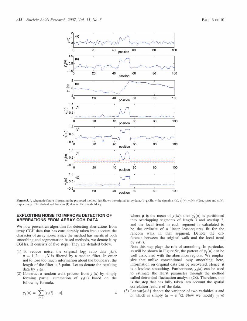
into overlapping segments of length 3 and overlap 2,and the local trend in each segment is calculated tobe the ordinate of a linear least-squares fit for therandom walk in that segment. Denote the dif-ference between the original walk and the local trendby y2(n).Note this step plays the role of smoothing. In particular,as will be shown in Figure 5c, the pattern of y

01ðnÞ can be

well-associated with the aberration regions. We empha-size that unlike conventional lossy smoothing, here,information on original data can be recovered. Hence, itis a lossless smoothing. Furthermore, y2(n) can be usedto estimate the Hurst parameter through the methodcalled detrended fluctuation analysis (28). Therefore, thisis the step that has fully taken into account the spatialcorrelation feature of the data.

(3) Let var{a,b} denote the variance of two variables a andb, which is simply (a � b)2/2. Now we modify y1(n)

Figure 5. A schematic figure illustrating the proposed method. (a) Shows the original array data, (b–g) Show the signals y1(n), y0

1ðnÞ, y2(n), y*1ðnÞ, y3(n) and y4(n),

respectively. The dashed red lines in (f) denote the threshold T1.

e35 Nucleic Acids Research, 2007, Vol. 35, No. 5 PAGE 6 OF 10

according to the following rule:

y*1ðnÞ y1ðnþ 1Þ‚ if varfy1ðnÞ‚y1ðn � 1Þg

> varfy1ðnÞ‚y1ðnþ 1Þg‚y*

1ðnÞ y1ðn � 1Þ‚ otherwise

8<: 5

Note this step does both segmentation and smoothing.(4) Let

y3ðnÞ ¼ y*1ðnÞ · y2ðnÞ‚

and define

y4ðnÞ ¼y*

1ðnÞ‚ if jy3ðnÞj > T1‚

y3ðnÞ‚ otherwise

�6

where T1 is a threshold value. This step yields a squarewave-like signal. With this signal, we can make simpledecisions, which is our step (5).

(5) Set thresholds T2 (a positive number) and T3 (a negativenumber), and identify the regions in y4(n) data greaterthan T2 or less than T3 as potential amplifications ordeletions in array CGH data. Sometimes in order toreduce false positives, we may discard small regions withonly one or two probes. However this should be donewith caution, since some microdeletions may onlycontain a single probe.

To make the above steps concrete, we have simulated anartificial chromosome data consisting of 100 probes, withthe centering 10 probes having aberrations. The simulateddata y(n) is shown in Figure 5a. Figure 5b–g show the signalsy1(n), y

01ðnÞ, y2(n), y*

1ðnÞ, y3(n) and y4(n), respectively. Thered dashed lines in Figure 5f correspond to a more or lessarbitrarily chosen threshold value T1.

Note all the three thresholds, T1, T2 and T3, can be definedby users. Also note that the ROC curves presented below donot depend on T1 sensitively. After we describe the conceptof p � SNR, we shall provide some guidelines as how tochoose T2 and T3.

We now compute the ROC curves for our method underthe same setting as when we discussed the CGHseg algorithm(Figure 4, green and purple curves). They are shown inFigure 4 as red and black curves, for array noise and Gaussiannoise, respectively. First we note that comparing with theresults of a recent comparison paper (23), our method iscomparable to the best smoothing based methods. Next, wemake two interesting observations from Figure 4: (i) TheROC curves for our method are very similar for the arraynoise and the Gaussian noise. This is because our methodhas fully taken into account the character of the arraynoise. (ii) Our method is more accurate than CGHseg, espe-cially when SNR is low and the aberration width is narrow.As we shall argue later, in the low SNR case, a good thresh-old to choose would correspond to the case of TPR +FPR ¼ 1. Under such a criterion, our method is almost20% more accurate than CGHseg, for the case of SNR ¼ 1and aberration width ¼ 5. Therefore, our method will beespecially useful for processing array CGH data with smallSNR [the 19 k oligo array data (24) belong to this category,as we shall show in the next section].

Next we examine the performance of our method fordetecting the boundaries of aberrations. Figure 6 compares

our result with those obtained using the CGHseg algorithm(15). The simulated data, shown in Figure 6a, consists of asingle aberration region, from 48 to 52. Due to fairly lowSNR, visually it is hard to tell which region might be theaberration region. However, our method correctly detectsboth the aberration region and the two breakpoints, asshown in Figure 6b. The CGHseg algorithm, however, doesnot seem to be able to cope with such low SNR data. Thisis evident in Figure 6c and d (as well as SupplementaryFigures 4–7): The CGHseg method may not only producefalse aberration regions, but also fail to detect boundarypoints correctly. The reason that our method works better isthat a few steps of our method have used smoothing. In par-ticular, the second step of our method is a lossless smoothing.No other methods have done so.

Finally, we evaluate our method by analyzing 15 BACarray data (2). Figure 7 compares aberration detection byusing our method shown in Figure 7a and b and the methodof Olshen and Vankatraman (12) shown in Figure 7c and d.The cell line is GM05296, with known aberrations on chro-mosomes 10 and 11. We observe that the two methods per-form similarly well. As will be explained later, these twodatasets have fairly high-SNR, and hence, aberration detec-tion is not too difficult.

POSTERIORI SIGNAL-TO-NOISE-RATIO (p � SNR)

We now consider an important question: after one appliesan algorithm to identify aberration regions and breakpointsfrom an array CGH data, how much confidence can onehave on the final result? When there are a lot of data avail-able, together with information on the background normalsituations, one may follow the procedure discussed byWang et al. (19). Here, we consider the more challengingcase of only one array data are available.

Our solution is quite simple. It amounts to utilizing theinformation summarized by ROC curves obtained by numeri-cal simulations as much as possible. From Figure 4, it is clearthat the accuracy of detection depends on two criticalparameters, the size of the aberration region and SNR. Infact, from Figure 4, it is clear that SNR is even more impor-tant than the size of the aberration region. Therefore, a goodstarting point would be to estimate SNR after one identifiesone or a few aberration regions. This can be achieved byusing the following simple formula:

p � SNR ¼ jmeanðaberrationÞ � meanðbackgroundÞjmax½STDðaberrationÞ‚STDðbackgroudÞ� ‚ 7

where p is used to emphasize that this is a posteriori esti-mation, and mean and STD denote mean and SD of thedata in the aberration region and background region (i.e.non-aberration region), respectively. When there are multipleaberration regions, p � SNR may be estimated for each aber-ration region identified. When this is the case, one needs totake the background region to be only around that aberrationregion. The p � SNR for the BAC array data (2) are listed inthe second column of Table 1. We observe that they are quitelarge, indicating that one can have high-confidence in thefinal detection results for the BAC array data (2). The p �SNR for the 385 k oligo array data http://www.nimblegen.

PAGE 7 OF 10 Nucleic Acids Research, 2007, Vol. 35, No. 5 e35

com/products/cgh/ are around 0.9 to 1.5, and are even smallerfor the 19 k oligo array data (24) (around 0.7–1.1). In particu-lar, we have estimated the p � SNR for the 385 k and 19 koligo array data based on the X chromosome using sex-mismatched samples. We have found that the p � SNR forthe two array platforms are 1.26 and 1.03, respectively,both falling in the range for each type of data listed above.Although we do not have access to the sex-mismatched Xchromosome data for the BAC array data (2), based on ouranalysis of the other two types of data, we have good reasonto believe that the p � SNR for the BAC array data’s sex-mismatched X chromosome would be at least around 3, there-fore, much larger than the p � SNR of the other two typesof data.

Our concept of p � SNR suggests that a good starting pointto choose the parameters T2 and T3 used in step (5) of ouralgorithm may correspond to signal intensity divided byp � SNR. This amounts to choosing one SD of the data.This rule suggests an iterative operation: starting fromarbitrarily chosen T2 and T3, calculate the correspondingp � SNR, then use the criterion discussed above to obtaina new estimate of T2 and T3, finally calculate the newp � SNR0. If p � SNR and p � SNR0 are similar, then thetwo parameters have been chosen appropriately.

We emphasize that our method works excellently if p �SNR is high. However, if p � SNR is low, then one maychoose threshold values that roughly yield TPR + FPR ¼ 1,where TPR and FPR define the ROC curve. In this case,

however, one should bear in mind that the classificationmay be incorrect with a probability of FPR.

DISCUSSION

In this paper, we have examined noise in array CGH dataof three resolution, the BAC array data, the 19 k and 385 koligo array data, and found that noise is highly non-Gaussianand possesses long-range spatial correlations. We have alsodeveloped a novel method for processing array CGH data.The method is a suitable combination of smoothing andsegmentation, and has fully taken into account the charac-teristics of noise in array CGH data. We have shown thatthe method is as accurate as the best smoothing-basedmethods for detecting aberration regions, and as accurate asthe best segmentation-based methods for finding boundarypoints. Furthermore, we have proposed a new concept,(p � SNR), to quantify the confidence level of aberrationregions and boundaries detected. We have found thatp � SNR for the 15 publicly available BAC array CGHdata are all quite large, indicating it is a relatively easy matterto accurately detect aberrations and boundaries from thosedata. However, p � SNR for the four 19k oligo arraydata are quite small, suggesting it is considerably morechallenging to detect aberrations from such array CGH data.

Although we have found that array CGH noise is highlynon-Gaussian with long-range spatial correlations, we do

Figure 6. Comparison of our result with those obtained using CGHseg algorithm (15). The aberration region consists of 5 probes, from 48 to 52. SNR is 2. (a)Shows the simulated data; this signal is also shown in (b–d) as blue dots. (b) Shows the result of our method. The red curve is y4(n), as explained in the procedure.The breakpoints 48 and 52 are both correctly detected; (c) Shows the result by CGHseg algorithm using heteroscedastic model, the estimated number of segmentsis K ¼ 3, while the breakpoints identified are 65 and 66; (d) Shows the result by CGHseg algorithm using homoscedastic model. The estimated number ofsegments is K ¼ 8, one of the two breakpoints, 48, is correctly detected. In (c and d), red lines represent the estimated mean of each segment, and green lines, theestimated mean plus or minus 1SD. To aid visual inspection, vertical dotted lines are drawn in (b–d).

e35 Nucleic Acids Research, 2007, Vol. 35, No. 5 PAGE 8 OF 10

not clearly know the mechanisms. A challenging task forfuture research would be to understand the biological mecha-nisms of such noise, as well as understand whether thosemechanisms are differentially related to different types ofdiseases.

Being able to identify smaller copy-number changes thataffect only a few probes is of particular importance in thefield of copy number polymorphism. This is because inher-ited, germ-line copy number variants are typically muchsmaller than rearrangements in cancer genomes. For example,two recent papers, one by McCarroll et al. (29), another byConrad et al. (30), identified a large class of inherited, multi-kilobase deletion polymorphisms that are predominantlysmaller than 20 kb in size. We emphasize that in order todetect small copy number changes, the key is to improvethe resolution of the array technology so that at least 2 pointscan be sampled for the region of interest. If only a single iso-lated point can be sampled, then it would be impossible byany analysis method to classify it as a true copy numberchange or just an outlier or noise.

Finally, readers interested in this method are stronglyencouraged to contact with the authors (e.g. gao@ece.ufl.edu)to obtain the source Matlab code.

ACKNOWLEDGEMENTS

Funding to pay the Open Access publication charges for thisarticle was provided by the Personalized Medicine Research

Program of Department of Medicine of Mount Sinai Schoolof Medicine.

Conflict of interest statement. None declared.

REFERENCES

1. Pinkel,D., Segraves,R., Sudar,D., Clark,S., Poole,I., Kowbel,D.,Collins,C., Kuo,W.L., Chen,C. and Zhai,Y. (1998) High resolutionanalysis of DNA copy number variation using comparative genomichybridization to microarrays. Nature Genet., 20, 207–211.

2. Snijders,A.M., Nowak,N., Segraves,R., Blackwood,S., Brown,N.,Conroy,J., Hamilton,G., Hindle,A.K., Huey,B. and Kimura,K. (2001)Assembly of microarrays for genome-wide measurement of DNA copynumber. Nature Genet., 29, 263–264.

3. Solinas-Toldo,S., Lampel,S., Stilgenbauer,S., Nickolenko,J.,Benner,A., Dohner,H., Cremer,T. and Lichter,P. (1997) Matrixbasedcomparative genomic hybridization: biochips to screen for genomicimbalances. Genes Chromosomes Cancer, 20, 399–407.

4. Ishkanian,A.S., Malloff,C.A., Watson,S.K., DeLeeuw,R.J., Chi,B.,Coe,B.P., Snijders,A., Albertson,D.G., Pinkel,D. and Marra,M.A.(2004) A tiling resolution DNA microarray with completecoverage of the human genome. Nature Genet., 36, 299–303.

5. Pinkel,D. and Albertson,D.G. (2005) Array comparative genomichybridization and its applications in cancer. Nature Genet., 37,s11–s17. Review.

6. Pollack,J.R., Sorlie,T., Perou,C.M., Rees,C.A., Jeffrey,S.S.,Lonning,P.E., Tibshirani,R., Botstein,D., Borresen-Dale,A.-L. andBrown,P.O. (2002) Microarray analysis reveals a major direct roleof DNA copy number alteration in the transcriptional programof human breast tumors. Proc. Natl Acad. Sci. USA, 99, 12963–12968.

7. Beheshti,B., Braude,I., Marrano,P., Thorner,P., Zielenska,M. andSquire,J.A. (2003) Chromosomal localization of DNA amplifications inneuroblastoma tumors using cDNA microarray comparative genomichybridization. Neoplasia, 5, 53–62.

Figure 7. Aberration detection using (a and b) our method and (c and d) the method of Olshen and Vankatraman (12). The cell line is GM05296, with knownaberrations on chromosomes 10 and 11. The dotted points are the original data. Red lines in (a and b) are the y4(n) signals explained in the procedure. Theyrepresent the estimated mean of each segment in (c and d). To aid visual inspection, vertical dotted lines are drawn in all the plots.

PAGE 9 OF 10 Nucleic Acids Research, 2007, Vol. 35, No. 5 e35

8. Hsu,L., Self,S.G., Grove,D., Randolph,T., Wang,K., Delrow,J.J.,Loo,L. and Porter,P. (2005) Denoising array-based comparativegenomic hybridization data using wavelets. Biostatistics, 6, 211–226.

9. Eilers,P.H.C. and de Menezes,R.X. (2005) Quantile smoothing of arrayCGH data. Bioinformatics, 21, 1146–1153.

10. Hodgson,G., Hager,J.H., Volik,S., Hariono,S., Wernick,M., Moore,D.,Nowak,N., Albertson,D.G., Pinkel,D., Collins,C. et al. (2001) Genomescanning with array CGH delineates regional alterations in mouse isletcarcinomas. Nature Genet., 29, 459–464.

11. Jong,K., Marchiori,E., Meijer,G., Vaart,A.V.D. and Ylstra,B. (2004)Breakpoint identification and smoothing of array comparative genomichybridization data. Bioinformatics, 20, 3636–3637.

12. Olshen,A.B., Venkatraman,E.S., Lucito,R. and Wigler,M. (2004)Circular binary segmentation for the analysis of array-based DNA copynumber data. Biostatistics, 5, 557–572.

13. Hupe,P., Stransky,N., Thiery,J.-P., Radvanyi,F. and Barillot,E. (2004)Analysis of array CGH data: from signal ratio to gain and loss of DNAregions. Bioinformatics, 20, 3413–3422.

14. Daruwala,R.-S., Rudra,A., Ostrer,H., Lucito,R., Wigler,M. andMishra,B. (2004) A versatile statistical analysis algorithm to detectgenome copy number variation. Proc. Natl Acad. Sci. USA, 101,16292–16297.

15. Picard,F., Robin,S., Lavielle,M., Vaisse,C. and Daudin,J.-J. (2005) Astatistical approach for array CGH data analysis. BMC Bioinformatics,6, 27.

16. Autio,R., Hautaniemi,S., Kauraniemi,P., Yli-Harja,O., Astola,J.,Wolf,M. and Kallioniemi,A. (2003) CGH-Plotter: MATLAB toolboxfor CGH-data analysis. Bioinformatics, 19, 1714–1715.

17. Myers,C.L., Dunham,M.J., Kung,S.Y. and Troyanskaya,O.G. (2004)Accurate detection of aneuploidies in array CGH and gene expressionmicroarray data. Bioinformatics, 20, 3533–3543.

18. Lingjaerde,O.C., Baumbusch,L.O., Liestol,K., Glad,I.K. andBorresen-Dale,A.-L. (2005) CGH-Explorer: a program for analysis ofarray-CGH data. Bioinformatics, 21, 821–822.

19. Wang,P., Kim,Y., Pollack,J., Narasimhan,B. and Tibshirani,R. (2005)A method for calling gains and losses in array CGH data. Biostatistics,6, 45–58.

20. Snijders,A.M., Fridlyand,J., Mans,D.A., Segraves,R., Jain,A.N.,Pinkel,D. and Albertson,D.G. (2003) Shaping of tumor anddrug-resistant genomes by instability and selection. Oncogene, 22,4370–4379.

21. Sebat,J., Lakshmi,B., Troge,J., Alexander,J., Young,J., Lundin,P.,Maner,S., Massa,H., Walker,M., Chi,M. et al. (2004) Large-scale copynumber polymorphism in the human genome. Science, 305,525–528.

22. Fridlyand,J., Snijders,A.M., Pinkel,D., Albertson,D.G. and Jain,A.(2004) Hidden Markov models approach to the analysis of array CGHdata. J Multivariate Anal., 90, 132–153.

23. Lai,W.R., Johnson,M.D., Kucherlapati,R. and Park,P.J. (2005)Comparative analysis of algorithms for identifying amplifications anddeletions in array CGH data. Bioinformatics, 21, 3763–3770.

24. Ziv,S., Brenner,O., Amariglio,N., Smorodinsky,N.I., Galron,R.,Carrion,D.V., Zhang,W.J., Sharma,G.G., Pandita,R.K. et al. (2005)Impaired genomic stability and increased oxidative stress exacerbatedifferent features of Ataxia-telangiectasia. Hum. Mol. Genet., 14,2929–2943.

25. Mandelbrot,B.B. (1982) The Fractal Geometry of Nature.W.H. Freeman, ISBN-10: 0716711869.

26. Gao,J.B., Hu,J., Tung,W.W., Cao,Y.H., Sarshar,N. andRoychowdhury,V.P. (2006) Assessment of long range correlation intime series: How to avoid pitfalls. Phys. Rev. E, 73, 016117.

27. Gao,J.B., Billock,V.A., Merk,I., Tung,W.W., White,K.D., Harris,J.G.and Roychowdhury,V.P. (2006) Inertia and memory in ambiguousvisual perception. Cogn. Process., 7, 105–112.

28. Peng,C.K., Buldyrev,S.V., Havlin,S., Simons,M., Stanley,H.E. andGoldberger,A.L. (1994) Mosaic organization of dna nucleotides. Phys.Rev. E, 49, 1685–1689.

29. McCarroll,S.A., Hadnott,T.N., Perry,G.H., Sabeti,P.C., Zody,M.C.,Barrett,J.C., Dallaire,S., Gabriel,S.B., Lee,C., Daly,M.J. andAltshuler,D.M. (2006) Common deletion polymorphisms in the humangenome. Nature Genet., 38, 86–92.

30. Conrad,D.F., Andrews,T.D., Carter,N.P., Hurles,M.E. andPritchard,J.K. (2006) A high-resolution survey of deletionpolymorphism in the human genome. Nature Genet., 38, 75–81.

e35 Nucleic Acids Research, 2007, Vol. 35, No. 5 PAGE 10 OF 10