e-theory and kk-theory for groups which act properly and ... kasparov - 2001... · e-theory and...
TRANSCRIPT

Digital Object Identifier (DOI) 10.1007/s002220000118Invent. math. 144, 23–74 (2001)
E-theory and KK-theory for groups which actproperly and isometrically on Hilbert space
Nigel Higson1,,Gennadi Kasparov2
1 Department of Mathematics, Pennsylvania State University, University Park, PA 16802,USA
2 Institut de Mathematiques de Luminy, CNRS – Luminy – Case 907, 163 Avenue deLuminy, 13288 Marseille Cedex 9, France
Oblatum 13-I-2000 & 14-IX-2000Published online: 8 December 2000 – Springer-Verlag 2000
1. Introduction
A good deal of research in C∗-algebra K -theory in recent years has beendevoted to the Baum-Connes conjecture [3], which proposes a formula forthe K -theory of group C∗-algebras that blends group homology with therepresentation theory of compact subgroups. The conjecture has brought C∗-algebra theory into close contact with manifold theory through its obvioussimilarity to the Borel conjecture of surgery theory [9,31] and its links withthe theory of positive scalar curvature [27]. In addition there are points ofcontact with harmonic analysis, particularly the tempered representationtheory of semisimple groups, although the proper relation between theBaum-Connes conjecture and representation theory is not well understood.
The conjecture is most easily formulated for groups which are discreteand torsion-free. For such a group G there is a natural homomorphism
µred : K∗(BG)→ K∗(C∗red(G)
),
mapping the K -homology of the classifying space of G to the K -theory ofthe reduced C∗-algebra of G (the reduced C∗-algebra is the completion ofthe complex group algebra of G in the regular representation as operatorson 2(G)). This assembly map is a counterpart of its namesake in surgerytheory, and, in line with the Borel conjecture, the Baum-Connes conjectureasserts that the assembly map is an isomorphism.
Nigel Higson was partially supported by an NSF grant. This research was partiallyconducted during the period Nigel Higson was employed by the Clay Mathematics Instituteas a CMI Prize Fellow.

24 N. Higson, G. Kasparov
The statement of the conjecture for discrete groups with torsion, orfor non-discrete groups, uses equivariant KK -theory [22]. Associated toany second countable, locally compact group G is a universal proper G-space EG, which is unique up to equivariant homotopy [3], and usingKK -theory we may form its equivariant K -homology K G∗ (EG). There isthen an assembly map
µred : K G∗ (EG)→ K∗
(C∗red(G)
)which is conjectured by Baum and Connes to be an isomorphism. For moredetails see [3].
The decoration ‘red’ – short for ‘reduced’ – is used because there is alsoan assembly map
µmax : K G∗ (EG)→ K∗
(C∗max(G)
)involving the full group C∗-algebra C∗max(G) (which is the enveloping C∗-algebra of the complex group algebra in the discrete case, and the envelop-ing C∗-algebra of L1(G) in general). This ‘max’ assembly map is notgenerally an isomorphism. Both the assembly maps µred and µmax may begeneralized by introducing a coefficient C∗-algebra A, on which G acts con-tinuously by C∗-algebra automorphisms. If the associated reduced crossedproduct C∗-algebra is denoted C∗red(G, A) then there is a reduced assemblymap
µred : KK G∗ (EG, A)→ K∗
(C∗red(G, A)
)defined again using KK -theory [3], along with a similar map µmax for thefull crossed product algebra C∗max(G, A).
The main purpose of this article is to prove the Baum-Connes conjec-ture for an interesting and fairly broad class of groups, called by Gromova-T-menable [10], and known to harmonic analysts as groups with theHaagerup approximation property [16]. These are those locally compactgroups which admit continuous, affine, isometric and metrically properactions on a Hilbert space, the latter term meaning that
limg→∞‖g · v‖ = ∞,
for every vector v in the Hilbert space. Gromov’s terminology is explainedby the twin facts that all (second countable) amenable groups admit suchan action [4], whereas no non-compact group with Kazhdan’s property Tdoes [13]. The Haagerup approximation property first arose in an investiga-tion of the Banach space structure of C∗-algebras [12].
Our main theorem is as follows.
KK-theory for groups which act properly on Hilbert space 25
1.1. Theorem. If G is a second countable, locally compact group, andif G has the Haagerup approximation property, then for any separableG-C∗-algebra A the Baum-Connes assembly maps
µred : KK G∗ (EG, A)→ K∗
(C∗red(G, A)
)and
µmax : KK G∗ (EG, A)→ K∗
(C∗max(G, A)
)are isomorphisms of abelian groups.
Remark. A recent article of Chabert, Echterhoff and Meyer [5] asserts thatthe definition of proper action used in the standard formulation of the Baum-Connes conjecture [3] agrees with the usual notion of a proper action ofa locally compact group on a locally compact space (this is obvious fordiscrete groups, but rather less clear otherwise). We shall use the latternotion throughout this paper.
Apart from amenable groups, important examples of groups coveredby Theorem 1.1 are free groups, the real and complex hyperbolic groupsSO(n, 1) and SU(n, 1), and Coxeter groups. A recent Seminaire Bourbakiof P. Julg [16] gives a good account of these and other examples. TheBaum-Connes conjecture was previously established for real and complexhyperbolic groups [21,17], but the argument we give here is quite differentin character. In fact, in view of the arguments used in [17] to prove theBaum-Connes conjecture for SU(n, 1), which blend contact geometry withunitary representation theory, it is quite remarkable that the arguments ofthis paper rely on essentially no geometry or representation theory at all.
Theorem 1.1 and a sketch of its proof, at least for discrete groups, werethe content of our recent announcement [14]. We shall give a full account ofthat argument, as it applies to the assembly mapµmax, in the first six sectionsof this paper. This much of Theorem 1.1 is sufficient for applications to theNovikov conjecture. Of course if G is amenable then µmax = µred, so wewill at this stage have completed the proof of Theorem 1.1 for discrete,amenable groups.
The arguments in [14] use asymptotic morphisms and E-theory [6,11],and unfortunately this theory is not well suited to dealing directly withµred. In our announcement we indicated an ad hoc way of circumventingthis problem. Here we shall follow a somewhat different course. A properG-C∗-algebra is a mildly non-commutative generalization of the notion ofa proper G-space (the algebra of continuous functions, vanishing at infinity,on a locally compact proper G-space is the prototypical example of a properG-C∗-algebra). It is proved in [11] that if G is discrete and A is proper thenthe assembly map
µmax : EG∗ (EG, A)→ K∗
(C∗max(G, A)
)

26 N. Higson, G. Kasparov
is an isomorphism. Roughly speaking, this is because proper actions arelocally modelled by actions of finite groups, while the Baum-Connes con-jecture is readily verified for finite groups. We used this result in our an-nouncement [14], by noting that if the C∗-algebra C (with trivial G-action)is isomorphic in equivariant E-theory to a proper G-C∗-algebra then everyseparable G-C∗-algebra B is E-theoretically a direct summand of a properG-C∗-algebra, so that the Baum-Connes assembly map for B, being a directsummand of the assembly map for a proper G-C∗-algebra, is an isomorph-ism. Here we shall use an improved result of Tu [29]: if the C∗-algebra C(with trivial G-action) is isomorphic in equivariant KK -theory to a properG-C∗-algebra then both of the Baum-Connes assembly maps µred and µmaxare isomorphisms, for any coefficient C∗-algebra.
The problem of showing that C is isomorphic in equivariant KK -theoryto a proper G-C∗-algebra reduces, as in [14], to Bott periodicity. If G actslinearly and isometrically on a finite-dimensional Hilbert space H then thetangent space TH is equivalent in equivariant K -theory to a point. If G actsproperly and affine-isometrically on H then the G-C∗-algebra C0(TH) isproper. Using the fact that any affine-isometric action on the flat Euclideanspace H is homotopic to a linear-isometric action, it follows that if G actsproperly and affine-isometrically on a finite-dimensional Euclidean spaceH then the proper G-C∗-algebra C0(TH) is equivalent in equivariant K -theory, and indeed in equivariant KK -theory, to C. We shall take the sameapproach in the infinite-dimensional case, following earlier work of ourswith J. Trout on the periodicity phenomenon in infinite dimensions [15].The main problems here are to find a suitable substitute for C0(TH), whichdoes not make sense in infinite dimensions, and to replicate Atiyah’s index-theoretic Bott periodicity argument [2] in the new context. The first problemwas solved in [15] and is reviewed here in Sect. 4. The requisite index theory,which is the heart of the matter, is developed in Sects. 2 and 3, and is appliedto our problem in the remaining sections of the paper.
To carry out the details of the above argument within KK -theory ratherthan E-theory (as was the case in [14] and [15]) we must recast our basic E-theory constructions in the language of KK -theory. The somewhat delicatearguments needed for this are presented in Sects. 7 and 8. Having done so,an attractive consequence presents itself:
1.2. Theorem. Every second countable, locally compact topological groupwith the Haagerup approximation property is K-amenable.
We shall not give the definition of K -amenability here (see [7,18]), butwe recall for the reader that it implies that at the level of K -theory there isno difference between C∗max(G, A) and C∗red(G, A). It follows that if G isK -amenable then the Baum-Connes assembly maps µmax and µred actuallycoincide. Thus if µmax is an isomorphism then so of course is µred.
It is a pleasure to thank George Skandalis for sharing with us his insightsinto one or two key arguments below. The second author would like to thank
KK-theory for groups which act properly on Hilbert space 27
the Shapiro Fund of the Pennsylvania State University for supporting a visitto State College, during which this project was initiated. The first authorwould like to thank the Department of Mathematics of the University Aix-Marseille II and the Institut de Mathematiques de Luminy for supportinga visit to Marseille during which the final parts of this paper were completed.
2. The Bott-Dirac operator in infinite dimensions
Let H be a separable, infinite-dimensional, real Hilbert space. The purposeof this section is to construct a certain Z/2-graded, complex Hilbert spaceH(H), comprised of differential forms on H . We shall also define a grading-degree one, index one, unbounded operator B on H(H) which is central tothe Bott periodicity phenomenon in infinite dimensions [15].
The complex Hilbert space H(H) will depend only on the affine struc-ture of H , and in fact we shall construct not one Hilbert space but an entirecontinuous field over the positive reals 0 < α <∞. These features will beused in later sections.
For any finite-dimensional, affine subspace V of H , we denote by V0 theunderlying vector subspace of H , comprised of differences of elements in V .We will call V a linear subspace of H if it contains the point 0 ∈ H . In thiscase V and V0 are one and the same. We will consider the exterior algebraΛ∗(V0) ⊗ C as endowed with its natural Euclidean structure, induced bythat of V0.
Fix a positive real number α.
2.1. Definition. (i) Let H(V ) be the Z/2-graded Hilbert space of square-integrable functions from V into Λ∗(V0)⊗ C.(ii) If W is a finite-dimensional linear subspace of H then denote by ξW ∈H(W ) the L2-normalized scalar function
ξW(w) = (πα)−m/4 exp(−‖w‖2/2α),
where m = dim(W ).(iii) If V ′ is an affine subspace of V , then the orthogonal complement W ofV ′ in V is defined as the orthogonal complement of V ′0 in V0. It is a linearsubspace. We define an isometry H(V ′)→ H(V ) by mapping f ∈ H(V ′)to the L2-form f(v′)·ξW (w). We regard the latter as a function of v = v′+w,where v′ ∈ V ′ and w ∈ W .
Notice that the isometry H(V ′)→ H(V ) depends on α > 0.If V ′′ ⊂ V ′ ⊂ V then the composition of isometries
H(V ′′)→ H(V ′)→ H(V )
is equal to the isometry associated to the inclusion V ′′ ⊂ V . This allows usto make the following construction:
28 N. Higson, G. Kasparov
2.2. Definition. Denote by H = H(H) the Hilbert space direct limit
H(H) = lim−→V⊂H
H(V ),
taken over the directed system of finite-dimensional affine subspaces of H ,using the isometries H(V ′) → H(V ) in Definition 2.1. Denote by ξH ∈H(H) the unit vector corresponding to any ξW ∈ H(W ) in the directedsystem, where W is any finite-dimensional linear subspace (all W producethe same ξH ).
The Hilbert space H(H) certainly depends on our choice of α > 0. Lateron, where necessary, we shall write Hα(H) in place of H(H) to indicatethis dependence.
Since the family of all finite-dimensional, affine subspaces of H is ratherunwieldy, we shall often use the following simple approximation result,whose proof is omitted.
2.3. Lemma. If H ′ is a dense subspace of H then the inclusion
lim−→V⊂H ′
H(V ) → lim−→V⊂H
H(V )
is an isomorphism of Hilbert spaces. In particular, if V1 ⊂ V2 ⊂ · · · is anincreasing family of finite-dimensional affine subspaces of H whose unionis dense in H then the canonical isometric inclusion of the Hilbert spacedirect limit lim−→H(Vn) into H(H) is a unitary isomorphism.
2.4. Definition. If W is a finite-dimensional linear subspace of H , and ifw ∈ W , then denote by ext(w) the operator of exterior multiplication by won Λ∗(W )⊗ C and by int(w) its adjoint (i.e. interior multiplication by w).The Clifford multiplication operators c(w) and c(w) are defined by
c(w) = ext(w)− int(w)c(w) = ext(w)+ int(w).
2.5. Definition. If V is a finite-dimensional affine subspace of H thendenote by s(V ) the dense Z/2-graded subspace of H(V ) comprised ofSchwartz functions from V into Λ∗(V0)⊗ C.
2.6. Definition. If W is a finite-dimensional linear subspace of H then wedefine a partial differential operator
BW : s(W )→ s(W )
by the formula
BW =m∑
i=1
αc(wi)∂
∂xi+ c(wi)xi,
KK-theory for groups which act properly on Hilbert space 29
where w1, . . . , wm is an orthonormal basis for W and x1, . . . , xm are coor-dinates in W dual to the orthonormal basis. This operator will be called theBott-Dirac operator on W .
The operator BW is independent of the choice of the basis w1, . . . , wmand is a symmetric, grading-degree one operator on s(W ). The square ofBW is
B2W =
m∑i=1
(−α2 ∂
2
∂x2i
+ x2i
)+ 2αN − αm,
where N is the operator which assigns to a differential form its degree. Itfollows from the well-known spectral theory for the harmonic oscillatorHamiltonian1 −α2d2/dx2 + x2 that the grading-degree zero and degreeone subspaces of s(W ) each contain an orthonormal basis comprised ofeigenfunctions for B2
W . The eigenvalues are 0, 2α, 4α, . . . ; each is of finitemultiplicity; and 0 occurs only in grading-degree zero, and with multiplicityone. The L2-normalized 0-eigenfunction is the function
ξW(w) = (πα)−m/4 exp(−‖w‖2/2α)
of Definition 2.1.It follows from the existence of an eigenbasis, or from standard facts
about first order linear partial differential operators, that BW is an essentiallyself-adjoint operator on the Hilbert space H(W ), with domain s(W ). It hascompact resolvent, and index one (in the graded sense of the word index).
Note that if W1,W2, . . . ,W j ⊂ W then we can certainly regard theoperators BW j as operators on s(W ). If W = W1 ⊕ · · · ⊕W j then
BW = BW1 + · · · + BW j
(the addition here refers to the ordinary sum of operators defined on thecommon domain s(W ); we are not concerned yet with the domains of theself-adjoint extensions of any of these operators). In addition it is easilyverified that Bi B j + B j Bi = 0 if i = j, so that
B2W = B2
W1+ · · · + B2
W j.
To define a Bott-Dirac operator on the whole of H we shall use thefollowing calculation.
1 For each n = 0, 1, 2, . . . the harmonic oscillator−α2d2/dx2 + x2 has an eigenfunction
of the form pn(x)e−x2/2α with eigenvalue (2n+ 1)α, where pn is a polynomial of degree n.
The lowest eigenfunction is e−x2/2α.
30 N. Higson, G. Kasparov
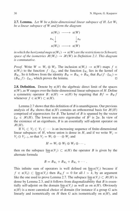
2.7. Lemma. Let W be a finite-dimensional linear subspace of H. Let W1be a linear subspace of W and form the diagram
s(W1) −−−→ s(W )
BW1
BW
s(W1) −−−→ s(W )
in which the horizontal maps s(W1 )→ s(W ) are the restrictions to Schwartzspace of the isometries H(W1)→ H(W ) in Definition 2.1. This diagramis commutative.
Proof. Write W = W1 ⊕ W2. The inclusion s(W1) → s(W ) maps f ∈s(W1) to the function f · ξW2, and the function ξW2 lies in the kernel ofBW2. So it follows from the identity BW = BW1 + BW2 that BW( f · ξW2) =(BW1 f ) · ξW2, which proves the lemma.
2.8. Definition. Denote by s(H) the algebraic direct limit of the spacess(W ), as W ranges over the finite-dimensional linear subspaces of H . Definea symmetric operator B : s(H) → s(H) by requiring that B f = BW fwhenever f ∈ s(W ) ⊂ s(H).
Lemma 2.7 shows that this definition of B is unambiguous. Our previousanalysis of BW shows that s(H) contains an orthonormal basis for H(H)comprised of eigenvectors for B. The kernel of B is spanned by the vectorξH ∈ H(H). The lowest non-zero eigenvalue of B2 is 2α. In view ofthe existence of an eigenbasis, B is an essentially self-adjoint operator onH(H).
If V1 ⊂ V2 ⊂ V3 ⊂ · · · is an increasing sequence of finite-dimensionallinear subspaces of H , whose union is dense in H , and if we write W j =Vj Vj−1, so that Vj = W1 ⊕ · · · ⊕W j and
H = W1 ⊕W2 ⊕W3 ⊕ · · · ,then on the subspace lim−→ s(Vj) ⊂ s(H) the operator B is given by thealternate formula
B = BW1 + BW2 + BW3 + · · · .This infinite sum of operators is well defined on lim−→ s(Vj) because iff ∈ s(Vk) ⊂ lim−→ s(Vj) then BWl f = 0 for all l > k, by an argumentlike the one used to prove Lemma 2.7. The subspace lim−→ s(Vj) ⊂ H(H) isdense by Lemma 2.3, and it follows from diagonalizability that B is essen-tially self-adjoint on the domain lim−→ s(Vj) as well as on s(H). Obviouslys(H) is a more canonical choice of domain (for instance if a group G actslinearly and isometrically on H then G acts isometrically on s(H), and
KK-theory for groups which act properly on Hilbert space 31
the operator B, defined on this domain, is equivariant). But lim−→ s(Vj) issometimes better suited to computations.
Because the operator B is so central to what follows, we conclude thissection with two other descriptions of it.
First, if w1, w2, . . . is an orthonormal basis for H , and if Vj is the spanof w1, . . . , w j , then on the subspace lim−→ s(Vj) ⊂ s(H) the operator B isgiven by the infinite series
B =∞∑
i=1
(αc(wi)
∂
∂xi+ c(wi)xi
).
As before, the infinite sum is well-defined since if η ∈ H(Vj) then η is inthe kernel of all the operators αc(wi)
∂∂xi+ c(wi)xi for i > j.
Second, if W is a finite-dimensional linear subspace of H then denoteby Ωalg(W ) the linear space of polynomial differential forms on W (in otherwords Ωalg(W ) is the linear span, within all differential forms on W , ofall polynomials on W , all de Rham differentials of polynomials, and allsums of products of these). If W1 ⊂ W then the operation of pull-backof differential forms along the orthogonal projection W → W1 defines anembedding Ωalg(W1)→ Ωalg(W ), and we define
Ωalg(H) = lim−→W⊂H
Ωalg(W ).
The de Rham differential gives a well-defined operator d : Ωalg(H) →Ωalg(H). Now define an inner product on Ωalg(H) by the formula
〈ω1, ω2〉 = (πα)− dim(W )/2∫
W(ω1, ω2)we−‖w‖
2/α dw (ω1, ω2 ∈ Ωalg(W )),
where (ω1, ω2)w denotes the pointwise inner product ofω1 andω2 atw ∈ W .The map ω → ω · ξW is an isometry from Ωalg(W ) into s(W ), and fromΩalg(H) into s(H).
2.9. Lemma. Under the inclusion Ωalg(H) ⊂ s(H) the Bott-Dirac oper-ator B on s(H) corresponds to the de Rham-type operator αd + αd∗ onΩalg(H) where d is the de Rham differential and d∗ denotes its formaladjoint with respect to the given inner product on Ωalg(H).
Remark. Part of the lemma is the assertion that the formal adjoint exists, asan operator on Ωalg(V ).
We shall not use the Lemma below. Its simple proof is left to the reader.
32 N. Higson, G. Kasparov
3. A non-commutative functional calculus for the operator B
If W is finite-dimensional then the resolvents (BW ± i)−1 of the Bott-Diracoperator are compact operators. This is no longer true in infinite dimensions,and the main purpose of this section is to introduce perturbations of the Bott-Dirac operator B for which this property is restored. Unfortunately theseperturbations destroy the symmetries of B, which is initially equivariant forany isometric linear action of a group on H . But we shall also investigatethe extent to which a limited form of equivariance is retained.
To accomplish these goals we shall introduce an interesting ‘functionalcalculus’ for B which associates to any self-adjoint (but not necessarilybounded) operator h on H a self-adjoint operator h(B) on H(H), in sucha way that for instance if h = I then h(B) = B, while if h has compactresolvent then so does h(B). The basic construction appears in our previouswork [14] and [15]. A recent article of Tu [30], extending our original workto groupoids, sketches a similar construction to the one below.
Our first definition of h(B) will require that h be diagonalizable. Laterwe will extend the definition to arbitrary h (see Definition 3.5).
3.1. Definition. Let h be a self-adjoint operator on the real Hilbert space H .Assumethath isdiagonalizable.Write H asanorthogonal sumofeigenspacesW j for h, and denote by λ j the corresponding eigenvalues. Let Vj =W1⊕· · ·⊕W j and define the operator h(B), acting on the space lim−→ s(Vj) ⊂H(H), by
h(B) = λ1 BW1 + λ2 BW2 + . . . .Remark. In the cases of most importance to us the eigenspaces W j will befinite-dimensional. But if some W j is infinite-dimensional then by BW j wewill of course mean the operator constructed by the direct limit procedureof the previous section.
By a calculation like the ones done in the previous section, when theinfinite sum
∑j λ j BW j is applied to any vector in lim−→ s(Vj) the result
has only finitely many non-zero terms. Hence there is no difficulty withconvergence of the sum in Definition 3.1.
3.2. Lemma. Let h be a self-adjoint diagonalizable operator on H. Thenthe operator h(B) is essentially self-adjoint. If h has compact resolvent thenh(B) also has compact resolvent.
Proof. We shall use the notation of Definition 3.1. In complete analogywith the case of B, the space lim−→ s(Vj) admits an orthonormal eigenbasis forh(B), therefore h(B) is essentially self-adjoint. If h has compact resolventthe each W j is finite-dimensional and the values λ2
j tend to infinity as jtends to infinity. The square of h(B) is
h(B)2 = λ21 B2
W1+ λ2
2 B2W2+ · · · ,

KK-theory for groups which act properly on Hilbert space 33
from which it follows that h(B)2 has an eigenbasis within lim−→ s(Vj) whoseeigenvalues are all sums
2n1λ21α+ 2n2λ
22α+ · · · ,
where n1, n2, . . . are non-negative integers, almost all zero. Associated toeach such sequence n1, n2, . . . there are finitely many eigenfunctions in theeigenbasis, so we see that
(1) the eigenvalues of the h(B)2 form a sequence converging to∞; and(2) each eigenvalue is of finite multiplicity.
The lemma follows immediately from this. In the following lemma, by the self-adjoint domain of an essentially
self-adjoint operator we mean the domain of its self-adjoint extension, or inother words the domain of its closure.
3.3. Lemma. Let h be a self-adjoint operator on H with compact resolvent,and suppose that h2 ≥ 1. Then the self-adjoint domain of h(B) is containedin the self-adjoint domain of B, and ‖h(B)ξ‖ ≥ ‖Bξ‖ for all vectors ξ inthe self-adjoint domain of h(B).
Proof. Let V1, V2, . . . be as in Definition 3.1. If ξ lies in lim−→S(Vj) then the
inequality ‖h(B)ξ‖2 ≥ ‖Bξ‖2 is clear from the formula for h(B)2 given inthe proof of Lemma 3.2, together with the fact that λ2
j ≥ 1, for all j. Theinequality ‖h(B)ξ‖2 ≥ ‖Bξ‖2 implies that the domain of the closure ofB contains the domain of the closure of h(B). Furthermore the inequalityextends by continuity to the domain of the closure of h(B).
To prove more about the operator h(B)we need an alternate descriptionwhich gives an explicit formula for h(B) on a larger domain than lim−→ js(Vj).Let h be any self-adjoint operator on H and let Hh ⊂ H be the domain of h.Denote by s(Hh) ⊂ s(H) the direct limit
s(Hh) = lim−→V⊂Hh
s(V )
over all finite-dimensional subspaces of Hh . We are going to define a sym-metric operator
h(B) : s(Hh)→ s(H)which, in the case where h is diagonalizable, will be an extension of the op-erator h(B) of Definition 3.1 (note that s(Hh) contains the domain lim−→ s(Vj)
given in Definition 3.1).

34 N. Higson, G. Kasparov
3.4. Definition. If W and V are finite-dimensional linear subspaces ofH then denote by s(W, V ) the Schwartz space of functions from W intoΛ∗(V ) ⊗ C. If W ′ ⊂ W and V ′ ⊂ V then the map f → f · ξW ′′ , whereW ′′ = W W ′, defines an isometry of s(W ′, V ′) into s(W, V ), just as inDefinition 2.1. Observe that
lim−→W,V⊂H
s(W, V ) = lim−→W⊂H
s(W ),
since the set of pairs (V, V ) is cofinal in the directed set of all pairs offinite-dimensional subspaces.
3.5. Definition. Let W be a finite-dimensional subspace of Hh and let V beany finite-dimensional subspace of H containing h[W]. Define an operator
h(BW ) : s(W,W )→ s(W, V )
by
h(BW ) =m∑
i=1
αc(hwi)∂
∂xi+ c(hwi)xi,
wherew1, . . . , wm is any orthonormal basis for W (the choice does not affectthe operator) and x1, . . . , xm are dual coordinates on W . As in Lemma 2.7and Definition 2.8, the formula
h(B)ξ = h(BW )ξ, ξ ∈ s(W )
unambiguously defines a symmetric operator
s(Hh) = lim−→W⊂Hh
s(W )h(B)−−−−→ lim−→
W,V⊂H
s(W, V ) = s(H).
3.6. Lemma. If h is a diagonalizable self-adjoint operator on H then therestriction of the symmetric operator h(B) : s(Hh) → s(H) to the directlimit lim−→ s(Vj) ⊂ s(Hh) of Definition 3.1 is the operator h(B).
Proof. If Vj is the direct sum of eigenspaces W1 ⊕ · · · ⊕W j for h, then bychoosing an orthonormal basis for V compatible with this decomposition itis clear that
h(BVj) = λ1 BW1 + · · · + λ j BW j .
The lemma follows immediately from this. Thus if h is diagonalizable then the operator h(B) is a symmetric exten-
sion of the essentially self-adjoint operator h(B) (and consequently has thesame closure). In view of this, henceforth we shall drop the tilde, and writeh(B) in place of h(B).

KK-theory for groups which act properly on Hilbert space 35
3.7. Lemma. If h is a bounded self-adjoint operator then ‖h(B)ξ‖ ≤‖h‖ · ‖Bξ‖, for every vector ξ ∈ s(H).Proof. Suppose first that h is diagonalizable, with eigenspaces W j , andeigenvalues λ j . Let Vj = W1 ⊕ · · · ⊕ W j . On the subspace lim−→ s(Vj) the
operator h(B)2 is the sum of the infinite series
h(B)2 = λ21 B2
W1+ λ2
2 B2W2+ · · · ,
while of courseB2 = B2
W1+ B2
W2+ · · · .
Since λ2j ≤ ‖h‖2 for all j, it follows easily that ‖h(B)ξ‖ ≤ ‖h‖‖Bξ‖ if
ξ ∈ lim−→ s(Vj). The inequality shows that the domain of the closure of B iscontained in the domain of the closure of h(B). Furthermore, by a continuityargument, the inequality extends to the domain of the closure of B. Since Bis essentially self-adjoint on lim−→ s(Vj), the domain of its closure certainlycontains s(H), and so the lemma is proved for diagonalizable operators.
A general bounded self-adjoint operator is a sum h1 + h2 of bounded,self-adjoint and diagonalizable operators, and we can even ensure that h2 hasnorm no more than any preassigned ε > 0. This follows, for instance, fromthe Weyl-von Neumann Theorem on diagonalizing self-adjoint operatorsmodulo compact operators. Since it is clear from Definition 3.5 that h(B) =h1(B) + h2(B) on s(H), it follows that ‖h(B)ξ‖ ≤ (‖h1‖ + ε)‖Bξ‖, andsince ε is arbitrarily small, the lemma follows.
3.8. Lemma. Let h1 and h2 be two self-adjoint operators on H which differby a bounded operator, and let Hh ⊂ H be their common domain. Assumethat h2
1 ≥ 1 and h22 ≥ 1. Then
‖h1(B)ξ − h2(B)ξ‖ ≤ ‖h1 − h2‖‖Bξ‖,for every ξ in s(Hh).
Proof. The difference h1(B) − h2(B) is the operator h(B), where h =h1 − h2. According to Lemma 3.3, s(Hh) ⊂ s(H). So this lemma followsfrom the previous one.
The following technical result will be called upon in Sect. 5.
3.9. Lemma. Let h1 and h2 be two positive, self-adjoint operators withcompact resolvent which differ by a bounded operator, and set
h1,α = 1+ αh1, B1,α = h1,α(B)h2,α = 1+ αh2, B2,α = h2,α(B).
Then limα→0 ‖ f(B1,α)− f(B2,α)‖ = 0, for any f ∈ C0(R).
36 N. Higson, G. Kasparov
Remark. When we use this lemma in Sect. 5 we shall want to think of B j,αas an unbounded operator on the Hilbert space Hα(H). The proof below isvalid whether or not the Hilbert space H(H) varies with α > 0.
Proof of the Lemma. By the Stone-Weierstrass Theorem, it suffices to provethe lemma for the function f(x) = (x + i)−1. By Lemma 3.8, if ξ ∈ s(Hh)then
‖B1,αξ − B2,αξ‖ ≤ α‖h1 − h2‖‖Bξ‖.If η belongs to the dense subspace (B1,α + i)s(Hh) ⊂ H(H) then
(B2,α + i)−1η− (B1,α + i)−1η = (B2,α + i)−1(B1,α − B2,α)(B1,α + i)−1η,
so if ξ = (B1,α + i)−1η ∈ s(Hh) then∥∥(B2,α + i)−1η− (B1,α + i)−1η∥∥ ≤ ‖B2,αξ − B1,αξ‖ ≤ α‖h1 − h2‖‖Bξ‖.
But since h21,α ≥ 1, it follows from Lemma 3.3 that ‖Bξ‖ ≤ ‖B1,αξ‖, and
so
‖Bξ‖2 ≤ ‖B1,αξ‖2 < ‖B1,αξ‖2 + ‖ξ‖2 = ‖(B1,α + i)ξ‖2 = ‖η‖2.
Therefore, ∥∥(B2,α + i)−1η− (B1,α + i)−1η∥∥ ≤ α‖h1 − h2‖‖η‖,
which proves the lemma.
Actually, we shall need a slight strengthening of the Lemma 3.9:
3.10. Lemma. With the notation of Lemma 3.9,
limα→0
sup ∥∥ f(s−1 B1,α)− f(s−1 B2,α)
∥∥ : s > 0 = 0
for any f ∈ C0(R).
Proof. The previous proof may be repeated verbatim, but with B1,α replacedby s−1 B1,α, and similarly for B2,α and B.
To illustrate the purpose of Lemma 3.9, let us note the following simpleconsequence:
KK-theory for groups which act properly on Hilbert space 37
3.11. Proposition. Suppose that a group G acts on H by linear isometries.Let h be a positive self-adjoint operator on H and suppose that g(h)− h isa bounded operator, for every g ∈ G. If Bα = hα(B), as in Lemma 3.9, then
limα→0
‖ f(Bα)− g( f(Bα))‖ = 0,
for every g ∈ G and f ∈ C0(R).
Thus despite the fact that h(B) is not equivariant, the operators hα(B)constitute a sort of ‘asymptotically equivariant’ family of operators.
Proof of the Proposition. Set h = h1 and g(h) = h2, and define B1,α andB2,α as in Lemma 3.9. Then since B is G-equivariant, g( f(B1,α) = f(B2,α).So the proposition follows immediately from Lemma 3.9. Remark. As in 3.10, it also follows that limα→0 ‖ f(s−1 Bα)− g( f(s−1 Bα))‖= 0, uniformly for s > 0. This will be used in Sect. 6.
This concludes that part of our discussion of the functional calculush → h(B)which is needed for this paper. But because it may be of interestelsewhere, we shall conclude this section with a further description ofh(B). Note first that for any subspace E ⊂ H we can define the Bott-Dirac operator BE : s(H) → s(H) to be the limit, as in Definition 2.8, ofoperators BV as V ranges over the finite-dimensional subspaces of E. Fortwo orthogonal subspaces E ′ and E ′′ in H , one has BE′+E′′ = BE′ + BE′′and B2
E′+E′′ = B2E′ + B2
E′′ .
3.12. Definition. Let h be a self-adjoint operator on H . Using the SpectralTheorem, let us write it in the integral form
h =∫ +∞
−∞t dPt
where dPt is a projection-valued measure on R. Thus h is the limit ofRiemann sums
∑k tk(Ptk+1 − Ptk). We define an operator h(B) on Hα as
the limit of the Riemann sums∑
k tk Bk where Bk is the operator BE for thesubspace E = Im(Ptk+1 − Ptk).
We leave to the reader the task of making precise and verifying theconvergence of the Riemann sums. Symbolically one can write:
h =∫ +∞
−∞t dPt, h(B) =
∫ +∞
−∞tBdPt H .
38 N. Higson, G. Kasparov
4. The C∗-algebra of a Hilbert space
In this section we shall review the construction in [15] of a certain non-commutative C∗-algebra associated to a real Hilbert space H . It plays therole of the algebra of continuous functions on the cotangent space of Hwhich vanish at infinity (note that if H is infinite-dimensional then thereare no non-zero, continuous functions on H which vanish at infinity, in theordinary sense of the term). The algebra described here differs very slightlyfrom the one introduced in [15]. In fact, we will use both the algebraintroduced in [15] and a new one which will be now defined.
Let V be a finite-dimensional affine subspace of H and, as in Sect. 2, letV0 be the associated vector subspace of H .
4.1. Definition. Denote by L(V ) the C∗-algebra of linear operators onthe finite-dimensional complex Hilbert space Λ∗(V0) ⊗ C. Observe thatΛ∗(V0) ⊗ C is a Z/2-graded Hilbert space, and so L(V ) is a Z/2-gradedC∗-algebra. Denote by Cliff (V ) the subalgebra of L(V ) generated by theClifford multiplication operators c(v) (defined in 2.4) for all v ∈ V .
4.2. Definition. Denote by C(V ) the Z/2-graded C∗-algebra C0(V0 × V,L(V )) of continuous, L(V )-valued functions on V0 × V which vanishat infinity, with the Z/2-grading induced from L(V ). Denote by C(V )the Z/2-graded C∗-algebra C0(V,Cliff (V )) of continuous, Cliff (V )-valuedfunctions on V which vanish at infinity, with the Z/2-grading induced fromCliff (V ).
The algebra C(V ) was used in [15]; it is the same as the algebra calledCτ (V ) in [22]. Here we will mainly use C(V ) (which is “twice bigger” thanC(V )) because it is better suited to the construction we will carry out in thenext section. Note that by a well-known isomorphism, L(V ) identifies withthe complex Clifford algebra of the Euclidean space V0 × V0 – this linksboth algebras.
4.3. Definition. Denote by S = C0(R) the C∗-algebra of continuouscomplex-valued functions on R which vanish at infinity. We shall con-sider S as Z/2-graded, according to even and odd functions. If A is anyZ/2-graded C∗-algebra then denote by S A the graded tensor product S⊗A.In particular, let SC(V ) = S⊗C(V ) and SC(V ) = S⊗C(V ). We will alsouse the following notation:
A(V ) = SC(V ), A(V ) = SC(V ).
Remark. One should think of the operation of graded tensor product with Sas encoding the grading information from C(V ) in the ungraded C∗-algebraA(V ). When we come to consider KK -theoretic invariants in Sect. 7, we
KK-theory for groups which act properly on Hilbert space 39
shall consider A(V ) and A(V ) as ungraded C∗-algebras (in other wordswe shall ignore their Z/2-grading). In Sect. 6, where E-theoretic invariantswill be discussed, one can consider these C∗-algebras either as graded or asungraded – both points of view are possible. But since the gradings will notplay any role at all the reader may perfectly well ignore them throughoutthe paper.
Now let V ′ be an affine subspace of V . Associated to the inclusionV ′ ⊂ V we are going to define a natural ∗-homomorphism A(V ′)→ A(V ).Having done so we will be able to define
A(H) = lim−→V⊂H
A(V ),
where the C∗-algebra direct limit is over the directed system of all finite-dimensional affine subspaces of H .
4.4. Definition. Suppose that W is a finite-dimensional linear subspaceof H . The Bott operator BW for C(W ) is the function BW : W × W →L(W ) whose value at (w1, w2) is the operator
ic(w1)+ c(w2) : Λ∗(W )⊗ C→ Λ∗(W )⊗ C(the Clifford multiplication operators c(w1) and c(w2) were introducedin Definition 2.4). The Bott operator is a grading-degree one, essentiallyself-adjoint, unbounded multiplier of C(W ), with domain the compactlysupported functions in C(W ). Using it, define a ∗-homomorphism A(0)→A(W ) by the formula
f → f(X⊗1+ 1⊗BW ),
where f ∈ S = A(0). Here X denotes the operator of multiplication by thefunction x onR, viewed as a degree one, essentially self-adjoint, unboundedmultiplier of S = C0(R) with domain the compactly supported functionsin S (see [15]). Similarly, in the case of A(W ), we can use the Bott operatorBW on Cliff (W ) given by the Clifford multiplication c(w) (which is thesecond variable part of the previous Bott operator) in order to define (by thesame formula) a ∗-homomorphism A(0)→ A(W ). (See again [15].)
Suppose now that V and V ′ are finite-dimensional affine subspaces of Hwith V ′ ⊂ V . There is a canonical inclusion L(V ′)→ L(V ) under whichthe Clifford operators c(v′) ∈ L(V ′) are mapped to the correspondingClifford operators c(v′) ∈ L(V ). So if we denote by p : V → V ′ theorthogonal projection then by composing with p we can transform anyfunction V ′ → L(V ′) to a function V → L(V ′), and hence to a functionV → L(V ). This gives a ∗-homomorphism from C(V ′) into the multiplieralgebra of C(V ) (but not into C(V ) itself, since the transformed functionswill not generally vanish at infinity).

40 N. Higson, G. Kasparov
Let W be the orthogonal complement of V ′0 in V0. There is similarlya canonical inclusion L(W )→ L(V ), and also a ‘projection’ q : V → Wdefined by q(v) = v − p(v). Using these, the Bott operator for W may beviewed as an unbounded multiplier of C(V ), and the operator X⊗1+1⊗BWas an unbounded multiplier of A(V ).
We can now define a ∗-homomorphism A(V ′)→ A(V ) by the formula:
A(V ′) = S⊗C(V ′) f ⊗h → f(X⊗1+ 1⊗BW ) · h ∈ A(V ).
Note that although generally neither of the multipliers f(X⊗1 + 1⊗BW )or h belongs to A(V ), the product always does.
The map A(V ′)→ A(V )may also be described as follows. The canoni-cal inclusions L(V ′)→ L(V ) and L(W )→ L(V ) induce an isomorphism
L(V ) ∼= L(W )⊗L(V ′),
and consequent isomorphisms
C(V ) ∼= C(W )⊗C(V ′)A(V ) ∼= A(W )⊗C(V ′).
We can now form a ∗-homomorphism
A(V ′) ∼= A(0)⊗C(V ′)→ A(W )⊗C(V ′) ∼= A(V )
by tensoring the Bott homomorphism of Definition 4.4 with the identity onC(V ′).
Quite similarly, there exists also a ∗-homomorphism A(V ′) → A(V )(see [15]).
4.5. Lemma. The ∗-homomorphisms A(V ′) → A(V ) we have just de-fined are transitive with respect to a triple of inclusions V ′′ ⊂ V ′ ⊂ V.
Proof. This is proved in [15, Proposition 3.2] for inclusions of linear sub-spaces; the proof for affine inclusions is just the same. 4.6. Definition. Define the C∗-algebras
A(H) = lim−→V⊂H
A(V ), A(H) = lim−→V⊂H
A(V ),
where the inductive limit is taken over the directed set of all finite-dimension-al affine subspaces of H .
As in Lemma 2.3, if H ′ is a dense subspace of H then the inclusion
lim−→V⊂H ′
A(V ) → lim−→V⊂H
A(V )
is an isomorphism of C∗-algebras. In particular, if V1 ⊂ V2 ⊂ · · · is anincreasing family of finite-dimensional affine subspaces of H , whose union
KK-theory for groups which act properly on Hilbert space 41
is dense in H , then the canonical isometric inclusion of lim−→A(Vn) into
A(H) is a unitary isomorphism. The same is true for A(H).We may regard V as a subspace of V0 × V via the embedding v →
(0, v). In the same way as in Definition 4.4, we define a ∗-homomorphismA(0) → A(V0) using the Bott operator on V0 which is the Clifford mul-tiplication operator ic(v) (i.e. the first variable part of the Bott operator ofDefinition 4.4). Now repeating the construction following Definition 4.4,we get an embedding A(V ) ⊂ A(V ) for any affine subspace V ⊂ H . Thetransitivity of the construction (similar to Lemma 4.5) guarantees that wecan pass to an inductive limit:
4.7. Lemma. The above procedure defines an embedding A(H) ⊂ A(H).
Suppose now that a second-countable, locally compact group G actscontinuously by affine isometries on the real Hilbert space H . Let us writethe action of G on H in the form:
g · v = π(g)v+ κ(g)where π is a linear orthogonal representation of G on H and κ is a one-cocycle on G with values in H . Thus κ is a continuous function from G intoH such that κ(g1g2) = π(g1)κ(g2)+ κ(g1).
The C∗-algebras A(H) and A(H) carry a natural action of our group G,and equipped with this action, they are G-C∗-algebra – that is, the action iscontinuous.
4.8. Definition. The affine isometric action of G on H is metrically properif limg→∞ ‖κ(g)‖ = ∞.
We recall from [11,14,22] that a G-C∗-algebra A is proper if there isa locally compact, second-countable, proper G-space Z and an equivariant∗-homomorphism from C0(Z) into the center of the multiplier algebra of Asuch that C0(Z) · A is dense in A.
4.9. Proposition. If G acts metrically properly on H then A(H) and A(H)are proper G-C∗-algebras.
Proof. The following elegant argument, which much improves our originalproof, is due to G. Skandalis. We will give the proof for A(H), the prooffor A(H) is similar.
For any non-zero, finite-dimensional affine subspace V ⊂ H , the centerZ(V ) of the C∗-algebra A(V ) is the algebra
Z(V ) = Sev ⊗ C0(V0 × V ),

42 N. Higson, G. Kasparov
where Sev is the subalgebra of all even functions in S. This algebra isisomorphic to the algebra of continuous functions, vanishing at infinity, onthe locally compact space [0,∞) × V0 × V . The maps of our inductivesystem, A(V ′) → A(V ), corresponding to embeddings V ′ ⊂ V , carrythese subalgebras into each other: Z(V ′) → Z(V ). So we can form thedirect limit Z(H). It has the property that Z(H) ·A(H) is dense in A(H).Its Gelfand spectrum is the locally compact space Z = [0,∞) × H × H ,where Z is given the weakest topology for which the projection to H × His weakly continuous and the function
Z = [0,∞)× H × H (t, v1, v2) → t2 + ‖v1‖2 + ‖v2‖2 ∈ Ris continuous. If G acts metrically properly on H then the induced actionon the locally compact space Z (which is the given affine action of G onthe second factor H and the linear part of this action on the first) is proper,in the ordinary sense of the term.
5. A continuous field of C∗-algebras associated to H
In Sect. 2 we fixed a scalar α > 0 and constructed from the real Hilbertspace H a complex Hilbert space of differential forms H(H). Let us nowmake the dependance of the complex Hilbert space H(H) on α explicit bywriting Hα(H).
The collection of all the Hilbert spaces Hα(H), for α > 0, constitutesa continuous field in a fairly obvious fashion: the space of continuous sec-tions is generated by the continuous functions ofα > 0 with values in H(V ),as V varies through the finite-dimensional affine subspaces of H . Associatedto the continuous field of Hilbert spaces Hα(H)0<α<∞ is the continuousfield of elementary Z/2-graded C∗-algebras K(Hα(H))0<α<∞.
5.1. Definition. Denote by Aα(H)0<α<∞ the continuous field of C∗-algebras obtained by tensoring the elementary field K(Hα(H))0<α<∞with the Z/2-graded C∗-algebra S = C0(R) of Definition 4.3. Thus
Aα(H) = SK(Hα(H)) = S⊗K(Hα(H)) (0 < α <∞).In addition, denote by A0(H) the C∗-algebra A(H) of Sect. 4.
Remark. We refer the reader to the article of Kirchberg and Wassermann [24]for a detailed discussion of tensor products and continuous fields of C∗-algebras. Kirchberg and Wassermann treat ungraded tensor products, where-as in our case the graded tensor product is used. But the elementary facts weneed – for instance that the tensor product of a continuous field by a nuclearC∗-algebra is again a continuous field – are not affected by the grading.

KK-theory for groups which act properly on Hilbert space 43
The aim of this section is to extend the continuous field Aα(H)0<α<∞to a continuous field of C∗-algebras Aα(H)0≤α<∞ over the closed halfline [0,∞).2 Here is how we shall do it. First we shall consider and solvethe same problem in finite dimensions, defining for each finite-dimensionalaffine subspace V of H a continuous field Aα(V )0≤α<∞. Next we shall fixa positive, self-adjoint operator h on H , with compact resolvent, and for eachfinite-dimensional affine space V lying within the domain of h we shall usethe functional calculus of Sect. 3 to define embeddings Aα(V )→ Aα(H)for all α ≥ 0. A continuous section of Aα(V )0≤α<∞ will then determinea section of Aα(H)0≤α<∞, and we shall deem that the sections obtainedin this way – which we shall call the basic sections of Aα(H)0≤α<∞ –generate all continuous sections of the field.
Because our construction depends on the compact-resolvent operator h,the field Aα(H)0≤α<∞ will not be canonical. However if a second-countable group G acts continuously on H by affine isometries then bychoosing h carefully we will obtain from our construction a G-continuousfield Aα(H)0≤α<∞, meaning that G acts continuously on each fiber alge-bra, and that the continuous sections of our field are transformed under G tocontinuous sections. In addition the field Aα(H)0≤α<∞ will be completelycanonical at the level of homotopy.
We begin by stating a well-known result in the realm of finite-dimen-sional spaces. Let V be a finite-dimensional affine subspace of H and forα ≥ 0 let C∗α(V0,C0(V )) be the crossed product C∗-algebra associated to theaction of the vector group V0 on the space V by the action v0 · v = αv0+ v.
5.2. Proposition. The crossed product algebras C∗α(V0,C0(V )) constitutethe fibers of a continuous field of C∗-algebras over [0,∞) in the followingway: each Schwartz function V0×V → C defines an element of each crossedproduct algebra C∗α(V0,C0(V )), and the sections so-obtained generate allthe continuous sections of C∗α(V0,C0(V ))0≤α<∞.
Remark. By ‘generate’ we mean that the continuous sections are preciselythose which are locally approximable by the above ‘constant’ sections, inthe same sense that a function is continuous if and only if it is locallyapproximable by constant functions.
Ifα = 0 then C∗α(V0,C0(V )) ∼= C0(V0×V ) via the Gelfand isomorphism
C∗(V0) ∼= C0(V0) ∼= C0(V0),
where V0 is identified with its Pontrjagin dual by means of the pairing(v1, v2) → exp(i〈v1, v2〉). If α > 0 then C∗α(V0,C0(V )) ∼= K(L2(V )), via
2 It is also possible [16] to extend the field to α = ∞, setting A∞(H) = A(0), but weshall not use this here.

44 N. Higson, G. Kasparov
the obvious representation of the crossed product on L2(V ). So Proposi-tion 5.2 provides us with a continuous field of the following sort:
C0(V0 × V ), α = 0,
K(L2(V )), α > 0.
5.3. Example. Suppose that f is a Schwartz function on V and let e be theGaussian e(v) = e−‖v‖2
on V0. Then by Fourier analysis, the prescriptione⊗ f ∈ C0(V0 × V ), α = 0,
e−α2∆M f ∈K(L2(V )), α > 0,
where ∆ is the Laplace operator on V and M f is the operator of point-wise multiplication by f , defines a continuous section, in fact a generating‘constant’ section, of the above continuous field.
Recall now that L(V ) denotes the C∗-algebra of endomorphisms of thefinite-dimensional Hilbert space Λ∗V0⊗C. Tensoring the above continuousfield with L(V ), we obtain a new continuous field
Cα(V ) =
C(V ), α = 0,K(H(V )), α > 0.
By further tensoring with S = C0(R) we obtain a continuous field
Aα(V ) =
A(V ), α = 0,SK(H(V )), α > 0.
Suppose now that V ′ ⊂ V . We are going to define an embedding ofcontinuous fields
Aα(V′)0≤α<∞ → Aα(V )0≤α<∞.
As usual, denote by W the orthogonal complement of V ′0 in V0, so that
V = W + V ′.
A pair ( fW , fV ′) of functions, one on W and one on V ′, determines a functionon V by the formula fV (w+v′) = fW (w) fV ′(v
′). This construction, togetherwith the isomorphism L(V ) ∼= L(W )⊗L(V ′) produces an isomorphism
H(V ) ∼= H(W )⊗H(V ′)
(compare Sect. 4). Thus
K(H(V )) ∼=K(H(W ))⊗K(H(V ′)).
KK-theory for groups which act properly on Hilbert space 45
Bearing in mind what was shown in Sect. 4, we see that there are isomor-phisms of continuous fields
Aα(V )0≤α<∞ ∼= Aα(W )⊗Cα(V′)0≤α<∞
and of course
Aα(V′)0≤α<∞ ∼= S⊗Cα(V
′)0≤α<∞for all α. So to define the required embedding of continuous fields we needonly embed the constant field with fiber S into the field Aα(W )0≤α<∞.This is done as follows:
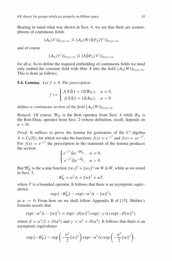
5.4. Lemma. Let f ∈ S. The prescription
f →
f(X⊗1+ 1⊗BW ), α = 0,
f(X⊗1+ 1⊗BW ), α > 0
defines a continuous section of the field Aα(W )0≤α<∞.
Remark. Of course, BW is the Bott operator from Sect. 4 while BW isthe Bott-Dirac operator from Sect. 2 (whose definition, recall, depends onα > 0).
Proof. It suffices to prove the lemma for generators of the C∗-algebraS = C0(R), for which we take the functions f(x) = e−x2
and f(x) = xe−x2.
For f(x) = e−x2the prescription in the statement of the lemma produces
the section e−x2⊗e−B
2W , α = 0,
e−x2⊗e−B2W , α > 0.
ButB2W is the scalar function ‖w1‖2+‖w2‖2 on W⊕W , while as we noted
in Sect. 3,B2
W = α2∆+ ‖w‖2 + αT,
where T is a bounded operator. It follows that there is an asymptotic equiv-alence
exp(−B2
W
) ∼ exp(−α2∆− ‖w‖2),
as α → 0. From here on we shall follow Appendix B of [15]. Mehler’sformula asserts that
exp(−α2∆− ‖w‖2) = exp(−β‖w‖2) exp(−γ∆) exp(−β‖w‖2),
where β = α2/2+ O(α4) and γ = α2 + O(α4). It follows that there is anasymptotic equivalence
exp(−B2
W
) ∼ exp
(−α
2
2‖w‖2
)exp(−α2∆) exp
(−α
2
2‖w‖2
),

46 N. Higson, G. Kasparov
as α → 0, and so the Fourier analysis calculation cited in Example 5.3shows that our section is continuous, as required.
The argument for the function f(x) = xe−x2is another direct calculation,
following Appendix B of [15] again. To summarize what we have shown: the embeddings S → Aα(W ) of
Lemma 5.4 produce an embedding of continuous fieldsAα(V
′)0≤α<∞ ∼= S⊗Cα(V′)
0≤α<∞
−→ Aα(W )⊗Cα(V
′)0≤α<∞ ∼= Aα(V )
0≤α<∞ .
Let us proceed now to the construction of embeddings
Aα(V ) −→ Aα(H) (0 ≤ α <∞).Let V be a finite-dimensional affine subspace of H and let V⊥ be theorthogonal complement of vector subspace V0 ⊂ H . If V ⊂ V1, and if W1 ⊂V⊥ is the orthogonal complement of V in V1, then we have already seenthat there is an isomorphism of Hilbert spaces H(V1) = H(W1)⊗H(V ).Passing to the direct limit we obtain an isomorphism
Hα(H) ∼= Hα(V⊥)⊗H(V ),
where on the right hand side Hα(V⊥) denotes the construction of Sect. 2,applied to the real Hilbert space V⊥. It follows that
K(Hα(H)) ∼=K(Hα(V⊥))⊗K(H(V )),
for every α > 0. Since it is also clear from Sect. 4 that
A(H) ∼= A(V⊥)⊗C(V ),
we obtain, for all α ≥ 0, isomorphisms
Aα(H) ∼= Aα(V⊥)⊗Cα(V)
analogous to those in the finite-dimensional case. Since
Aα(V ) ∼= S⊗Cα(V ),
it is natural to attempt to define embeddings Aα(V )→ Aα(H) by meansof embeddings S → Aα(V⊥), using for the latter the formula
f →
f(X⊗1+ 1⊗BV⊥), α = 0,
f(X⊗1+ 1⊗BV⊥), α > 0
as in the finite-dimensional case, where f(X⊗1+ 1⊗BV⊥) now means theelement of A(V⊥) associated to f ∈ S = A(0) by the canonical inclusionA(0)→ A(V⊥). Unfortunately the Bott-Dirac operator BV⊥ does not havecompact resolvent, and so for α > 0 the formula does not define an element
KK-theory for groups which act properly on Hilbert space 47
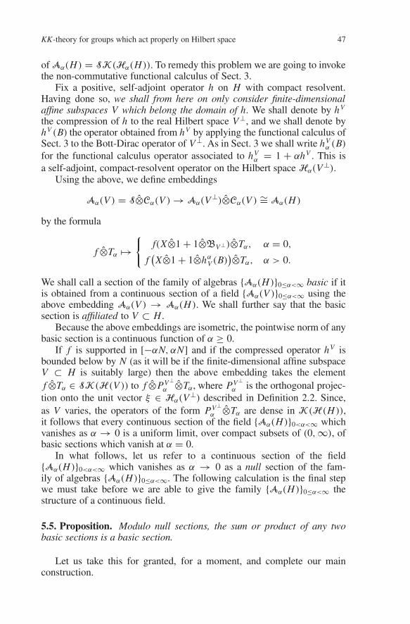
of Aα(H) = SK(Hα(H)). To remedy this problem we are going to invokethe non-commutative functional calculus of Sect. 3.
Fix a positive, self-adjoint operator h on H with compact resolvent.Having done so, we shall from here on only consider finite-dimensionalaffine subspaces V which belong the domain of h. We shall denote by hV
the compression of h to the real Hilbert space V⊥, and we shall denote byhV (B) the operator obtained from hV by applying the functional calculus ofSect. 3 to the Bott-Dirac operator of V⊥. As in Sect. 3 we shall write hV
α (B)for the functional calculus operator associated to hV
α = 1 + αhV . This isa self-adjoint, compact-resolvent operator on the Hilbert space Hα(V⊥).
Using the above, we define embeddings
Aα(V ) = S⊗Cα(V )→ Aα(V⊥)⊗Cα(V ) ∼= Aα(H)
by the formula
f ⊗Tα →
f(X⊗1+ 1⊗BV⊥)⊗Tα, α = 0,
f(X⊗1+ 1⊗hαV (B)
)⊗Tα, α > 0.
We shall call a section of the family of algebras Aα(H)0≤α<∞ basic if itis obtained from a continuous section of a field Aα(V )0≤α<∞ using theabove embedding Aα(V ) → Aα(H). We shall further say that the basicsection is affiliated to V ⊂ H .
Because the above embeddings are isometric, the pointwise norm of anybasic section is a continuous function of α ≥ 0.
If f is supported in [−αN, αN] and if the compressed operator hV isbounded below by N (as it will be if the finite-dimensional affine subspaceV ⊂ H is suitably large) then the above embedding takes the elementf ⊗Tα ∈ SK(H(V )) to f ⊗PV⊥
α ⊗Tα, where PV⊥α is the orthogonal projec-
tion onto the unit vector ξ ∈ Hα(V⊥) described in Definition 2.2. Since,as V varies, the operators of the form PV⊥
α ⊗Tα are dense in K(H(H)),it follows that every continuous section of the field Aα(H)0<α<∞ whichvanishes as α → 0 is a uniform limit, over compact subsets of (0,∞), ofbasic sections which vanish at α = 0.
In what follows, let us refer to a continuous section of the fieldAα(H)0<α<∞ which vanishes as α → 0 as a null section of the fam-ily of algebras Aα(H)0≤α<∞. The following calculation is the final stepwe must take before we are able to give the family Aα(H)0≤α<∞ thestructure of a continuous field.
5.5. Proposition. Modulo null sections, the sum or product of any twobasic sections is a basic section.
Let us take this for granted, for a moment, and complete our mainconstruction.

48 N. Higson, G. Kasparov
5.6. Definition. A section of the family of algebras Aα(H)0≤α<∞ is con-tinuous if it is a uniform limit, over compact subsets of [0,∞), of basicsections.
The continuous sections do indeed constitute the continuous sectionsfor a continuous field: the pointwise norm of any continuous section isa continuous function (because, as noted above, this is true for the basicsections); the continuous sections form an algebra over the continuousfunctions on [0,∞) (by Proposition 5.5 and the preceding discussion aboutnull sections); and every element of every algebra Aα(H) is the value at αof some continuous section.
Proof of Proposition 5.5. Since the finite-dimensional affine subspaces Vof the domain of h form a directed set under inclusion, and since the sumand product of any two basic sections which are affiliated to a single finite-dimensional affine subspace are obviously basic, it suffices to show that ifV ⊂ V1 ⊂ domain (h) then any basic section which is affiliated to V isequal to a basic section affiliated to V1, modulo a null section. In addition, itsuffices to prove this for a basic section affiliated to an ‘elementary’ sectionof Aα(V )0≤α<∞ of the type f ⊗Tα. We have previously constructed anembedding of Aα(V )0≤α<∞ into Aα(V1)0≤α<∞, and if we apply first thisembedding to the section f ⊗Tα, and then the embedding of Aα(V1)0≤α<∞into Aα(H)0≤α<∞, we obtain the section
f(X⊗1+ 1⊗hV1
α (B))⊗Tα ∈ S⊗K(H(V⊥))⊗K(H(V )).
In the formula the operator hV1 (which is, to begin with, the compressionof h to V⊥1 ⊂ V⊥) is regarded as an operator on V⊥ by setting hV1 equalto zero on the orthogonal complement of V⊥1 in V⊥. On the other hand, thebasic section associated directly to f ⊗Tα is
f(X⊗1+ 1⊗hV
α (B))⊗Tα ∈ S⊗K(H(V⊥))⊗K(H(V )).
Comparing the two formulas, and bearing in mind that the operators hV andhV1 on V⊥ differ by a bounded operator, we see that the proposition followsfrom Lemma 3.9.
Suppose now that a second-countable, locally compact group G actson the real Hilbert space H by a continuous, affine and isometric action.Then G also acts on the continuous field K(Hα(H))0<α<∞, and henceon Aα(H)0<α<∞, in the sense that each g ∈ G transforms each contin-uous section of Aα(H)0<α<∞ to another continuous section. Of course,G also acts on the algebra A0(H) = A(H) of Sect. 4. Let us now addressthe question of whether G acts on the continuous field Aα(H)0≤α<∞ inDefinition 5.6.

KK-theory for groups which act properly on Hilbert space 49
5.7. Lemma. Let G be a second countable, locally compact group andsuppose that G acts continuously on a real, separable Hilbert space H byaffine isometries g · v = π(g)v + κ(g). There exists a positive, self-adjointoperator h on H with compact resolvent such that κ(g) ∈ domain (h) andπ(g)h − hπ(g) is bounded, for any g ∈ G. In particular, the domain of h isG-invariant.
Remark. We shall say that an operator h as in the lemma is adapted to theaffine action of G on h.
Proof. Let V1, V2, V3, . . . be any increasing sequence of finite-dimensionalsubspaces of H whose union is dense in H . Let K1 ⊂ K2 ⊂ ... ⊂ G bean exhaustive system of compact subsets of G. We can define inductivelya subsequence Vn1 ⊂ Vn2 ⊂ ... ⊂ H such that the orthogonal projectionsPn1, Pn2, ... onto these subspaces have the properties that
‖(1− Pn j )κ(K j)‖ ≤ 2− j
and‖(1− Pn j+1)π(K j)Pn j‖ ≤ 2− j .
Put h =∑∞j=0(1− Pn j ) (with Pn0 = 0). It is clear that κ(G) belongs to the
domain of this operator. If Qn j = Pn j − Pn j−1 then h = ∑j nQn j , which
clearly has compact resolvent. The operator hπ(g)−π(g)h can be written inthe form:
∑k> j (k− j)(Qnkπ(g)Qn j −Qn jπ(g)Qnk). Estimating separately
the two parts of this sum corresponding to k = j + 1 and k > j + 1 we findthat hπ(g) − π(g)h is bounded. This implies that domain (h) is invariantunder the linear part π of the G-action. But since κ(G) ⊂ domain (h), thelast assertion follows. 5.8. Proposition. Let G be a second countable, locally compact groupwhich acts continuously on a real, separable Hilbert space H by affineisometries. If h is a positive, self-adjoint, compact-resolvent operator onthe Hilbert space H which is adapted to the action of G then the fieldAα(H)0≤α<∞ constructed from h is G-continuous.
Remark. One might in addition ask whether G acts continuously on the C∗-algebra of continuous sections of Aα(H)0≤α<∞ which vanish at+∞. Thisis so, and is a consequence of the Baire category theorem. See Theorem 1.1.4of [28].
Proof of the Proposition. It suffices to show that the image of a basicsection under an affine isometry g is, modulo null sections, again a basicsection. But if we apply g to a basic section of the form
f(X⊗1+ 1⊗hV
α (B))⊗Tα ∈ S⊗K(H(V⊥))⊗K(H(V )).
we obtain the section
f(X⊗1+ 1⊗h V
α (B))⊗g(Tα) ∈ S⊗K(H(V⊥))⊗K(H(V )),

50 N. Higson, G. Kasparov
where V = gV and h = π(g)hπ(g−1). Observe that since h is adapted tothe action of G on H , the affine space V belongs to the domain of h and theoperator h is a bounded perturbation of h. So it follows from Lemma 3.9that the latter section is equal to the basic section
f(X⊗1+ 1⊗hV
α (B))⊗g(Tα) ∈ S⊗K(H(V⊥))⊗K(H(V )),
modulo null sections. The dependence of the field Aα(H)0≤α<∞ on the operator h is not
important because of the following:
5.9. Proposition. Let G be a second countable, locally compact group andsuppose that G acts continuously on a real, separable Hilbert space Hby linear isometries. If h0 and h1 are two positive, self-adjoint operatorson H with compact resolvent, and if both are adapted to the action of Gon H, then there exists a G-equivariant, continuous field of C∗-algebrasAα,t(H) over [0,∞)×[0, 1]whose restrictions to 0 ∈ [0, 1]and 1 ∈ [0, 1]are the continuous fields constructed, as in Definition 5.6 from h0 and h1,respectively.
Proof. Let us say that operators h0 and h1 are compatible if there is sucha field. Note that compatibility is an equivalence relation.
If h0 and h1 have a common eigenbasis then the linear path ht of op-erators between h0 and h1, thought of as a path of operators defined onthe algebraic span of the common eigenbasis for h0 and h1, consists ofessentially self-adjoint operators. Indeed the path determines a single es-sentially self-adjoint, compact resolvent operator k on the Hilbert moduleH ⊗ C[0, 1] over C[0, 1] which is adapted to the affine action of G onH ⊗ C[0, 1]. Applying the construction of Definition 5.6 to each operatorin the family ht (or alternatively to k in the context of Hilbert modules)we see that h0 and h1 are compatible.
In the general case, fix eigenbases for H associated to the operators h0and h1, and choose an orthogonal operator T mapping the eigenbasis forh0 bijectively to that of h1. Since the orthogonal group of a Hilbert space isconnected (in the strong, or even the norm topology), there is a path joiningT to the identity operator. It follows that there exists a continuous familyof orthonormal bases for H , parametrized by t ∈ [0, 1], which is at t = 0the eigenbasis for h0 and at t = 1 the eigenbasis for h1. Let us regard thisfamily of orthonormal bases as an orthonormal basis for the Hilbert moduleH⊗C[0, 1]. Starting with the subspaces Vn spanned by the first n-elementsof our eigenbasis for H ⊗ C[0, 1], the same construction as in the proof ofLemma 5.7 gives a self-adjoint, compact resolvent operator k on this Hilbertmodule which is adapted to the action of G on H ⊗ C[0, 1]. Applying theconstruction of Definition 5.6 to k we see that k0 and k1 are compatible. Butthe operator k, restricted to t = 0, commutes with h0 while the operatork, restricted to t = 1, commutes with h1. It follows that h0 is compatiblewith h1, as required.

KK-theory for groups which act properly on Hilbert space 51
6. The Dirac and dual Dirac elements in E-theory
In this section we shall use ideas from the theory of asymptotic morphismsto construct ‘Dirac’ and ‘dual Dirac’ elements in E-theory. We shall thenbe able to prove the E-theoretic version of the Baum-Connes conjecture,at least for discrete groups which act properly and isometrically on Hilbertspace, and for the assembly map µmax. To fully prove the results stated inSect. 1 we shall need to translate our constructions from E-theory to KK -theory. Because this translation is in places rather delicate we shall need tocarry out the present E-theoretic calculations in a somewhat more refinedcontext than would otherwise be necessary.
Let G be a second countable, locally compact topological group and letA and B be separable G-C∗-algebras.
6.1. Definition. (See [5], [11], [28].) An equivariant asymptotic morphismfrom A to B is a family of functions ϕtt∈[1,∞) : A → B such that:
• t → ϕt(a) is bounded and norm-continuous on [1,∞), for any a ∈ A;• (g, a) → g(ϕt(a)) is norm-continuous in g ∈ G and a ∈ A, uniformly in
t ∈ [1,∞); and• for every a, a1, a2 ∈ A, g ∈ G and α ∈ C,
limt→∞
ϕt(a1a2)− ϕt(a1)ϕt(a2)
ϕt(a1 + a2)− ϕt(a1)− ϕt(a2)
ϕt(αa)− αϕt(a)ϕt(a
∗)− ϕt(a)∗
ϕt(g(a))− g(ϕt(a))
= 0.
We shall usually indicate an asymptotic morphism as above by thenotation ϕ : A→→B. The apparently restrictive uniform continuity conditionin the definition is really quite innocent: see Proposition 1.1.3 of [28].
Obviously, an equivariant ∗-homomorphism ϕ : A → B determines anequivariant asymptotic morphism for which ϕt = ϕ, for all t. Slightly lesstrivial is the assertion that an asymptotically G-equivariant family of ∗-homomorphisms ϕt : A → B, where by ‘asymptotically G-equivariant’ wemean that ϕt(g(a))− g(ϕt(a))→ 0 pointwise, as t →∞, is an equivariantasymptotic morphism from A to B. Uniform continuity in a and g followsfrom Theorem 1.1.4 of [28].
One of the two main constructions in the theory of asymptotic morphismsassociates to any extension of separable G-C∗-algebras
0 → J → E → A → 0
an asymptotic morphism ϕ : ΣA→→J , where ΣA = C0(0, 1) ⊗ A. Recallfirst the following notion:

52 N. Higson, G. Kasparov
6.2. Definition. A continuous quasicentral approximate unit for a separa-ble G-C∗-algebra E containing an ideal J is a continuous family ut1≤t<∞of positive elements in the unit ball of J for which
• limt→∞ ‖ut x − x‖ = 0, for every x ∈ J;• limt→∞ ‖ut x − xut‖ = 0 for every x ∈ E; and• limt→∞ ‖g(ut)− ut‖ = 0 uniformly on compact subsets of G.
See [11], Lemma 6.3 or [28], Lemma 1.2.1, for the existence of such fam-ilies in the case of separable C∗-algebras. The following lemma describesthe asymptotic morphism associated to an extension:
6.3. Lemma. (See [6], Lemma 10; [11], Proposition 6.5; [28], Lemma 1.2.2.)Given an extension
0 → J → E → A → 0
of separable G-C∗-algebras, let s : A → E be an arbitrary cross-section(not necessarily linear, or equivariant, or even continuous) and ut a con-tinuous quasicentral approximate unit for E. There exists an asymptoticmorphism ϕ : ΣA→→J such that ϕt( f ⊗ a) is asymptotically equivalent tof(ut)s(a), for every f ∈ Σ = C0(0, 1) and every a ∈ A.
We will call this asymptotic morphism ϕ : ΣA→→J the central asymp-totic morphism associated to the above extension. Of course it depends onthe choice of continuous quasicentral approximate unit ut, and to be ac-curate, even given ut, Lemma 6.3 only determines the central asymptoticmorphism ϕ : ΣA→→J up to asymptotic equivalence. But its homotopyclass is well-defined, where homotopy is defined via asymptotic morphismsA→→B[0, 1].
A commutative diagram
0 −−−→ J1 −−−→ E1 −−−→ A1 −−−→ 0 0 −−−→ J2 −−−→ E2 −−−→ A2 −−−→ 0
in the category of separable G-C∗-algebras and equivariant ∗-homomorph-isms gives rise to a homotopy-commutative diagram
ΣA1→→J1 ΣA2→→J2
of asymptotic morphisms and ∗-homomorphisms. See [28], 1.2.10 and1.2.11; or [11], 6.8. The construction of the central asymptotic morphismis normalized in the following way: the central asymptotic morphism
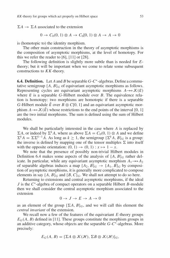
KK-theory for groups which act properly on Hilbert space 53
ΣA → ΣA associated to the extension
0 → C0(0, 1)⊗ A → C0[0, 1) ⊗ A → A → 0
is (homotopic to) the identity morphism.The other main construction in the theory of asymptotic morphisms is
the composition of asymptotic morphisms, at the level of homotopy. Forthis we refer the reader to [6], [11] or [28].
The following definition is slightly more subtle than is needed for E-theory; but it will be important when we come to relate some subsequentconstructions to KK -theory.
6.4. Definition. Let A and B be separable G-C∗-algebras. Define a commu-tative semigroup A, BG of equivariant asymptotic morphisms as follows.Representing cycles are equivariant asymptotic morphisms A→→K(E)where E is a separable G-Hilbert module over B. The equivalence rela-tion is homotopy: two morphisms are homotopic if there is a separableG-Hilbert module E over B ⊗ C[0, 1] and an equivariant asymptotic mor-phism A→→K(E) whose restrictions to the end points of the interval [0, 1]are the two initial morphisms. The sum is defined using the sum of Hilbertmodules.
We shall be particularly interested in the case where A is replaced byΣA, or indeed by Σk A, where as above ΣA = C0(0, 1)⊗ A and we defineΣk A = ΣΣk−1 A. As long as k ≥ 1, the semigroup Σk A, BG is a group:the inverse is defined by mapping one of the tensor multiples Σ into itselfwith the opposite orientation: (0, 1)→ (0, 1) : x → 1− x.
We note that the presence of possibly non-trivial Hilbert modules inDefinition 6.4 makes some aspects of the analysis of A, BG rather del-icate. In particular, while any equivariant asymptotic morphism A1→→A2of separable algebras induces a map A2, BG → A1, BG by composi-tion of asymptotic morphisms, it is generally more complicated to composeelements in say A, BG and B,CG. We shall not attempt to do so here.
Returning to extensions and central asymptotic morphisms, if the idealJ is the C∗-algebra of compact operators on a separable Hilbert B-modulethen we shall consider the central asymptotic morphism associated to theextension
0 → J → E → A → 0
as an element of the group ΣA, BG , and we will call this element thecentral invariant of the extension.
We recall now a few of the features of the equivariant E-theory groupsEG(A, B) defined in [11]. These groups constitute the morphism groups inan additive category, whose objects are the separable G-C∗-algebras. Moreprecisely:
EG(A, B) = ΣA ⊗K(H ),ΣB ⊗K(H )G,
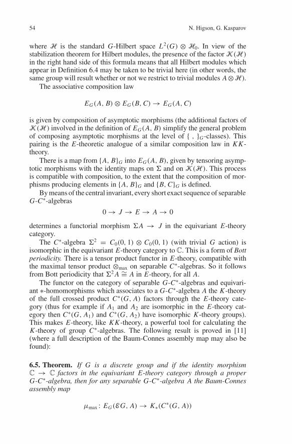
54 N. Higson, G. Kasparov
where H is the standard G-Hilbert space L2(G) ⊗ H0. In view of thestabilization theorem for Hilbert modules, the presence of the factor K(H )in the right hand side of this formula means that all Hilbert modules whichappear in Definition 6.4 may be taken to be trivial here (in other words, thesame group will result whether or not we restrict to trivial modules A⊗H).
The associative composition law
EG(A, B)⊗ EG(B,C)→ EG(A,C)
is given by composition of asymptotic morphisms (the additional factors ofK(H ) involved in the definition of EG(A, B) simplify the general problemof composing asymptotic morphisms at the level of , G-classes). Thispairing is the E-theoretic analogue of a similar composition law in KK -theory.
There is a map from A, BG into EG(A, B), given by tensoring asymp-totic morphisms with the identity maps on Σ and on K(H ). This processis compatible with composition, to the extent that the composition of mor-phisms producing elements in A, BG and B,CG is defined.
By means of the central invariant, every short exact sequence of separableG-C∗-algebras
0 → J → E → A → 0
determines a functorial morphism ΣA → J in the equivariant E-theorycategory.
The C∗-algebra Σ2 = C0(0, 1) ⊗ C0(0, 1) (with trivial G action) isisomorphic in the equivariant E-theory category toC. This is a form of Bottperiodicity. There is a tensor product functor in E-theory, compatible withthe maximal tensor product ⊗max on separable C∗-algebras. So it followsfrom Bott periodicity that Σ2 A ∼= A in E-theory, for all A.
The functor on the category of separable G-C∗-algebras and equivari-ant ∗-homomorphisms which associates to a G-C∗-algebra A the K -theoryof the full crossed product C∗(G, A) factors through the E-theory cate-gory (thus for example if A1 and A2 are isomorphic in the E-theory cat-egory then C∗(G, A1) and C∗(G, A2) have isomorphic K -theory groups).This makes E-theory, like KK -theory, a powerful tool for calculating theK -theory of group C∗-algebras. The following result is proved in [11](where a full description of the Baum-Connes assembly map may also befound):
6.5. Theorem. If G is a discrete group and if the identity morphismC → C factors in the equivariant E-theory category through a properG-C∗-algebra, then for any separable G-C∗-algebra A the Baum-Connesassembly map
µmax : EG(EG, A)→ K∗(C∗(G, A))

KK-theory for groups which act properly on Hilbert space 55
is an isomorphism. If C∗red(G) is an exact C∗-algebra then the same hy-potheses imply that the assembly map
µred : EG(EG, A)→ K∗(C∗red(G, A)
)is also an isomorphism. Remark. We recall that a C∗-algebra D is exact if tensoring by D, usingthe minimal C∗-algebra tensor product, preserves short exact sequences. Itis known that if G is a discrete subgroup of a connected Lie group thenC∗red(G) is exact. See [25].
We shall now apply the above information to prove the isomorphism ofµmax (and of µred in the exact case) for any discrete group which admitsa metrically proper affine isometric action on a Hilbert space. The caseof non-discrete, or non-exact, groups will be the subject of the remainingsections.3
Let G be a second-countable, locally compact group acting properly andisometrically on a real Hilbert space H .
6.6. Definition. The dual Dirac element β ∈ S, A(H)G is the classin the group S, A(H)G of the asymptotically G-equivariant family of∗-homomorphisms ϕt : S = A(0) → A(H) defined by composing theembedding ϕ : A(0) → A(H) associated to the inclusion 0 → H withthe ∗-homomorphisms S → S induced from the family of contractionsx → t−1x on R. Thus ϕt( f ) = ϕ( ft), where ft(x) = f(t−1x). Exactlythe same definition applies also to the algebra A(H) and gives an elementβ ∈ S,A(H)G which we will also call the dual Dirac element. Note thatthe element β is the image of β under the natural embedding A(H) →A(H) constructed in Lemma 4.7. We shall sometimes also use the term‘dual-Dirac element’ to refer to the asymptotic morphism, as opposed to itshomotopy class.
Let h be a compact-resolvent, positive self-adjoint operator on the Hilbertspace H which is adapted to the action of G on H , as in Lemma 5.7. As inSect. 5, associated to h there is a continuous field Aα(H)0≤α<∞. Let usdenote by Fh (H) the C∗-algebra of continuous sections of the field Aα(H)which vanish at α = ∞. Evaluation at α = 0 produces an extension of G-C∗-algebras
0 →K(S⊗E )→ Fh(H)→ A(H)→ 0,
in which E denotes the Hilbert C0(0,∞)-module of sections of the field ofHilbert spaces Hα(H) which vanish both at α = 0 and α = ∞, and S⊗E
3 The case of non-discrete groups could probably be handled by appropriately extendingthe results of [29] from KK -theory to E-theory. The case of non-exact groups could behandled within E-theory as in [14], but as explained in the introduction we shall obtain animproved result in the coming sections.

56 N. Higson, G. Kasparov
is the corresponding Hilbert module over SΣ = S⊗C0(0,∞). (We identifyhere Σ = C0(0, 1) with C0(0,∞) via an orientation preserving continuousmonotone map (0, 1)→ (0,∞).)
6.7. Definition. The Dirac element α ∈ ΣA(H),SΣG is the centralinvariant of the extension
0 →K(S⊗E )→ Fh(H)→ A(H)→ 0
just described. The Dirac element α ∈ ΣA(H),SΣG is the restrictionof α to the subalgebra A(H) of A(H). (We shall sometimes also use theterm ‘Dirac element’ to refer to the asymptotic morphism rather than to itshomotopy class.)
We noted in Proposition 5.9 that the homotopy class of the above exten-sion does not depend on h. As a result, two different choices for h producethe same Dirac element.
The Dirac and dual Dirac elements determine classes α ∈ EG(ΣA(H),SΣ) and Σβ ∈ EG(ΣS,ΣA(H)) (the latter by tensoring the dual Diracasymptotic morphism by an additional copy of Σ). We are going to provethe following result:
6.8. Theorem. The E-theory composition
ΣSΣβ−−→ ΣA(H)
α−→ SΣ
of the Dirac and dual Dirac morphisms is equal in E-theory to the transpo-sition isomorphism τ : ΣS → SΣ. The same is also true for A(H) in placeof A(H).
Bearing in mind Proposition 4.9 and Theorem 6.5, we will obtain thefollowing immediate consequence:
6.9. Corollary. Let G be a countable discrete group which admits a metri-cally proper, affine-isometric action on a Hilbert space. For any separableG-C∗-algebra A the Baum-Connes assembly map
µmax : EG(EG, A)→ K∗(C∗(G, A))
is an isomorphism. If C∗red(G) is an exact C∗-algebra then the same hy-potheses imply that the assembly map
µred : EG(EG, A)→ K∗(C∗red(G, A)
)is also an isomorphism.
Actually, with the requirements of the coming sections in mind, we shallprove a more precise version of Theorem 6.8:
KK-theory for groups which act properly on Hilbert space 57
6.10. Theorem. The composition of asymptotic morphisms
α ·Σβ : ΣS→→ΣA(H)→→K(SE )
is equal to the homotopy class of the transposition map 1 : ΣS → SΣ inthe group ΣS,SΣG.
Remark. This theorem certainly implies Theorem 6.8.
Proof of Theorem 6.10. In view of the observations made in Definitions 6.6and 6.7, it is enough to prove the assertion for A(H). The assertion for A(H)will follow.
Write the affine, isometric action of G as
g · v = π(g)v+ κ(g),where π is a linear, orthogonal representation of G on H . In order to provethat the composition α ·Σβ is equal to 1, let us consider a family of affineG-actions
gs · v = π(g)v+ sκ(g),
parametrized by s ∈ [0, 1]. Observe that when s = 1 we recover theinitial affine action, whereas when s = 0 the action is linear. Denote byA(H)s the C∗-algebra A = A(H), but with the scaled G-action (g, a) →gs(a). The algebras A(H)s form a continuous field of G-C∗-algebras overthe unit interval, and we shall denote by A(H)[0, 1] the G-C∗-algebra ofcontinuous sections. In a similar way, form a continuous field of G-C∗-algebras K(SE )s = K(SE ) (we are abbreviating S⊗E to SE) and denoteby K(SE )[0, 1] the G-C∗-algebra of continuous sections. There are obvious[0, 1]-parametrized versions of the dual Dirac and Dirac elements, and theircomposition
ΣS→→ΣA[0, 1]→→K(SE )[0, 1]provides a homotopy between the composition α · Σβ for the initial affineaction of G and the same composition α ·Σβ for the linear one. This meansthat in order to prove that the composition α ·Σβ is equal to 1, it is enoughto consider the case of a linear action of G on H .
In the case of a linear action the natural embedding S → A(H) de-fined by the identification S % A(0) is G-equivariant. Let us consider anextension of G-algebras
0 →K(SE )→ F Sh → S → 0
which is the pull-back of the basic extension
0 →K(SE )→ Fh(H)→ A(H)→ 0
along the embedding S → A(H). By functoriality of the central invariant,the composition α ·Σβ coincides with the central invariant ΣS→→K(SE )of the pull-back extension. So it is enough to prove that the central invariantof the latter extension is the element τ in ΣS,SΣG .
58 N. Higson, G. Kasparov
Recall now the operation of sum for extensions of G-C∗-algebras (seefor instance [20], Sect. 7). When we have two extensions,
0 →K(Ei)→ Di → A → 0 (i = 1, 2),
where E1 and E2 are Hilbert modules over B, the sum of the two extensionsis the extension
0 → K(E1 ⊕ E2)→ D⊕ → A → 0,
where D⊕ is an algebra of matrices of the type:
(d1 k12k21 d2
), with di ∈ Di
and kij ∈K(Ei,E j), such that d1 and d2 are mapped to the same element ofA (and the map of D⊕ → A is defined by assigning just this element to theabove matrix). The central invariant of a sum of two extensions is equal tothe sum of central invariants.
In the present case, the pull-back extension that we are trying to analyzeis the sum of the unit extension
0 → S ⊗ C0(0,∞)→ S ⊗ C0[0,∞)→ S → 0,
whose central invariant is τ , and the extension
0 → PK(SE )P → PF Sh P → S → 0,
where P is the orthogonal projection onto the orthogonal complement ofthe kernel of the Bott-Dirac operator. To complete the proof of the theoremwe must show that the central invariant of this extension is zero.
If f ∈ S and s > 0 then define fα,s ∈ SK(Hα(H)) by the formula
fα,s = f(X⊗1+ 1⊗s−1hα(B)
).
For a given s, the fα,s determine an element in F Sh , and indeed of PF S
h Pby compression. If DS
h is the C∗-algebra generated by the functions
(0, 1] s → fs ∈ PF Sh P
together with the functions from (0, 1] into K(SE ) which vanish at 0, thenwe obtain an equivariant extension
0 → C0(0, 1] ⊗ PK(SE )P → DSh → S → 0
(equivariance of the extension follows from Lemma 3.10 and the remarkfollowing 3.11). Restricting to s = 1 gives a commutative diagram
0 −−−→ C0(0, 1] ⊗ PK(SE )P −−−→ DSh −−−→ S −−−→ 0 =
0 −−−→ PK(SE )P −−−→ PF Sh P −−−→ S −−−→ 0
,
so the required triviality of the central invariant for the bottom row followsfrom functoriality of the central invariant and homotopy invariance.
KK-theory for groups which act properly on Hilbert space 59
One can also calculate the composition of the Dirac and dual Diracelements in the reverse order. We will not use this calculation in the proofof the main results of this paper. For this reason, we give here only a sketchof the proof of the following theorem.
6.11. Theorem. The composition (β ⊗ 1) · α of asymptotic morphisms:
ΣA(H)→→SK(E )→→A(H)⊗K(E ),
is equal to the homotopy class of the transposition map in ΣA(H),A(H)⊗ΣG. The same is also true for A(H) in place of A(H).
Sketch of proof. We will give the proof for the algebra A(H). The prooffor A(H) is similar. The argument is based on the existence of a naturalextension of C∗-algebras:
0 → K(A(H)⊗E )→ Fh(H × H)→ A(H × H)→ 0.
To produce this extension, one needs to change a little bit the construc-tion described in Sect. 5. We start with the continuous field of C∗-alge-bras A(H)⊗K(Hα(H)). We construct embeddings A(V )⊗Cα(V ) →A(H)⊗K(Hα(H)) in the same way as was done in the definition of a basicsection but taking into account one more tensor variable which comes fromA(V ). The rest of the construction is the same as in Sect. 5. Let us denotethe central invariant of the resulting extension by ζ .
Consider now an embedding: H → H × H given by h → (0, h).This embedding is not equivariant but it gives rise to a natural asymptoticmorphism ϕt : A(H)→ A(H × H) defined by
ϕt( f ⊗T ) = f(X⊗1+ t−1(1⊗BH )
)⊗T
whereBH is the Bott element for the first copy of H . It is easy to show thatthe composition ζ · ϕt is homotopic to the composition (β ⊗ 1) · α.
We can now use the rotation trick of Atiyah [2]. Let us apply the rotationhomotopy of H×H given by the usual 2×2 matrix. It interchanges the twovariables in H×H . The embedding H → H×H becomes now h → (h, 0).So the asymptotic morphism ϕt transforms into the asymptotic morphismϕ′t given essentially by the same formula but in which BH is already theBott element for the second copy of H .
We can now apply the same argument as in the proof of the previoustheorem. Over the second variable H , it is possible to make a homotopyof the group action to the linear one. After that, our embedding A(H)→A(H × H) will become G-equivariant. Moreover, the extension we haveconstructed at the beginning of the proof will become the sum of twoextensions. The rest of the proof is similar to the proof of Theorem 6.10.
60 N. Higson, G. Kasparov
7. Asymptotic morphisms and KK-theory
In this section and the next we shall carry out the project of transferring thearguments of the previous section from E-theory to KK -theory (our basicreference for KK -theory is [22]). We will work in the category of triviallygraded C∗-algebras. Our aim is to be able to apply to a-T-menable groupsthe following result of J.-L. Tu ([29], Theorem 2.2; see also [5] and theproof of Theorem 14.1 in [11]), which strengthens Theorem 6.5:
7.1. Theorem. Let G be a second countable, locally compact and Haus-dorff topological group, and let A be a separable, proper G-C∗-algebra.If there are elements x ∈ KK G(C, A) and y ∈ KK G(A,C) such thatx ⊗A y = 1C in KK G(C,C) then for every separable G-C∗-algebra B theBaum-Connes assembly map
µred : KK G(EG, B)→ K∗(C∗red(G, B)
)is an isomorphism. In addition, G is K-amenable.
Suppose that G acts isometrically on a real Hilbert space H . In Sect. 8we will construct a ‘dual Dirac element’ b ∈ KK G
1 (C,A(H)). Under theadditional hypothesis that the action of G on H is proper we shall alsoconstruct a ‘Dirac element’ d ∈ KK G
1 (A(H),C). Of course, we should liketo show that b ⊗A(H ) d = 1 in KK G(C,C). Unfortunately the argumentwe used in Sect. 6 to settle the analogous point in E-theory involved notonly the given proper action on H but also the associated linear action,and the natural homotopy between them. Since the linear action is certainlynot proper (except in the trivial case where G is compact) the E-theoryargument does not readily transfer to KK -theory.
The essential problem here is that while there is a natural transformation
KK G(A, B)→ EG(A, B),
there is in general no natural transformation the other way round. But asa partial substitute we shall define and analyze homomorphisms
ρ : Σ2, BG → KK G0 (C, B)
andρ : Σ, BG → KK G
1 (C, B).
Using them we shall eventually be able to reduce the calculation b⊗A(H ) d= 1 to the analogous asymptotic morphism calculation, which we alreadydid in Theorem 6.10.
We will start by studying maps in the reverse direction and reformulat-ing the construction of the central asymptotic morphism associated to anextension (see Lemma 6.3). As we have already said above, we will assumethat all considered C∗-algebras are trivially graded.
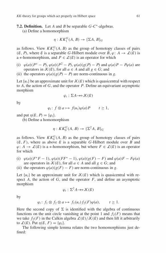
KK-theory for groups which act properly on Hilbert space 61
7.2. Definition. Let A and B be separable G-C∗-algebras.(a) Define a homomorphism
η : KK G1 (A, B)→ ΣA, BG
as follows. View KK G1 (A, B) as the group of homotopy classes of pairs
(E, P), where E is a separable G-Hilbert module over B, ϕ : A → L(E ) isa ∗-homomorphism, and P ∈ L(E) is an operator for which
(i) ϕ(a)(P∗ − P), ϕ(a)(P2 − P), ϕ(a)(g(P)− P) and ϕ(a)P − Pϕ(a) areoperators in K(E), for all a ∈ A and all g ∈ G; and
(ii) the operators ϕ(a)(g(P)− P) are norm-continuous in g.
Let ut be an approximate unit for K(E )which is quasicentral with respectto A, the action of G, and the operator P. Define an equivariant asymptoticmorphism
ϕt : ΣA→→K(E)
byϕt : f ⊗ a → f(ut)ϕ(a)P t ≥ 1,
and put η(E, P) = ϕt.(b) Define a homomorphism
η : KK G0 (A, B)→ Σ2 A, BG
as follows. View KK G0 (A, B) as the group of homotopy classes of pairs
(E, F), where as above E is a separable G-Hilbert module over B andϕ : A → L(E ) is a ∗-homomorphism, but where F ∈ L(E ) is an operatorfor which
(i) ϕ(a)(F∗F − 1), ϕ(a)(FF∗ − 1), ϕ(a)(g(F) − F) and ϕ(a)F − Fϕ(a)are operators in K(E), for all a ∈ A and all g ∈ G; and
(ii) the operators ϕ(a)(g(F) − F) are norm-continuous in g.
Let ut be an approximate unit for K(E ) which is quasicentral with re-spect A, the action of G, and the operator F, and define an asymptoticmorphism
ϕt : Σ2 A→→K(E)
byϕt : f1 ⊗ f2 ⊗ a → f1(ut) f2(F)ϕ(a), t ≥ 1.
Here the second copy of Σ is identified with the algebra of continuousfunctions on the unit circle vanishing at the point 1 and f2(F) means thatwe take f2(F) in the Calkin algebra L(E)/K(E) and then lift it arbitrarilyto L(E). Put η(E, F) = ϕt.
The following simple lemma relates the two homomorphisms just de-fined:

62 N. Higson, G. Kasparov
7.3. Lemma. When A = ΣA1, the homomorphism η on KK G1 (A, B)
coincides up to sign with the homomorphism η on KK G0 (A1, B), after
KK G0 (A1, B) and KK G
1 (A, B) are identified by Bott Periodicity.
Remark. We note that the periodicity isomorphisms in KK -theory areunique, up to sign, so there is no need to specify them in the above as-sertion.
We now introduce the promised homomorphisms ρ which associateKK -theory classes to asymptotic morphisms.
7.4. Definition. Let B be a separable G-C∗-algebra.(a) Define a homomorphism
ρ : Σ, BG → KK G0 (C, B ⊗ C0(0,∞)) ∼= KK G
1 (C, B)
as follows. Let E be a separable G-Hilbert module over B and let ϕt :Σ→→K(E) be an equivariant asymptotic morphism. For t ≤ 1, defineϕt = tϕ1 and then extend ϕt unitally to the unitalized algebra Σ to obtaina unital map:
ϕt : Σ→ L(E ⊗ C0(0,∞)).Set Vt = ϕt(v), where v is the generator of the algebra Σ, which weconsider as the algebra of continuous functions on the unit circle. Theelement V = Vt ∈ L(E ⊗ C0(0,∞)) satisfies the conditions:
VV ∗ − 1, V ∗V − 1, g(V )− V ∈ K(E ⊗ C0(0,∞)), ∀g ∈ G,
and we define ρ(ϕt) to be the corresponding element of KK G0 (C, B ⊗
C0(0,∞)).(b) Similarly, we define a homomorphism
ρ : Σ2, BG → KK G1 (C, B ⊗ C0(0,∞)) ∼= KK G
0 (C, B)
as follows. Let ϕt : Σ2→→K(E ) be an equivariant asymptotic morphism.
For t ≤ 1 define ϕt = tϕ1; extend ϕt unitally to unitalized algebra Σ2; andthen pass to matrices to obtain a unital map
ϕt : M2(Σ2)→ M2(L(E ⊗ C0(0,∞))).Set Pt = ϕt(p), where the element
p = 1
1+ |z|2(
1 zz |z|2
)∈ M2(Σ2)
is the canonical rank-one projection, the algebra Σ2 being identified withthe algebra of continuous functions on the Riemann sphere and z being
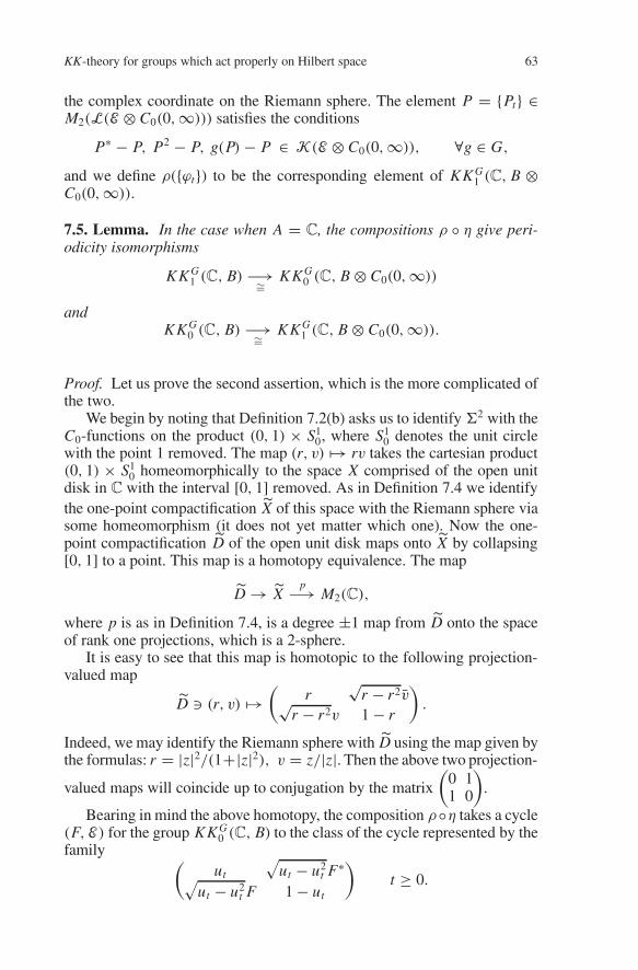
KK-theory for groups which act properly on Hilbert space 63
the complex coordinate on the Riemann sphere. The element P = Pt ∈M2(L(E ⊗ C0(0,∞))) satisfies the conditions
P∗ − P, P2 − P, g(P)− P ∈ K(E ⊗ C0(0,∞)), ∀g ∈ G,
and we define ρ(ϕt) to be the corresponding element of KK G1 (C, B ⊗
C0(0,∞)).7.5. Lemma. In the case when A = C, the compositions ρ η give peri-odicity isomorphisms
KK G1 (C, B) −→∼= KK G
0 (C, B ⊗ C0(0,∞))and
KK G0 (C, B) −→∼= KK G
1 (C, B ⊗ C0(0,∞)).
Proof. Let us prove the second assertion, which is the more complicated ofthe two.
We begin by noting that Definition 7.2(b) asks us to identify Σ2 with theC0-functions on the product (0, 1) × S1
0, where S10 denotes the unit circle
with the point 1 removed. The map (r, v) → rv takes the cartesian product(0, 1) × S1
0 homeomorphically to the space X comprised of the open unitdisk in C with the interval [0, 1] removed. As in Definition 7.4 we identifythe one-point compactification X of this space with the Riemann sphere viasome homeomorphism (it does not yet matter which one). Now the one-point compactification D of the open unit disk maps onto X by collapsing[0, 1] to a point. This map is a homotopy equivalence. The map
D → Xp−→ M2(C),
where p is as in Definition 7.4, is a degree ±1 map from D onto the spaceof rank one projections, which is a 2-sphere.
It is easy to see that this map is homotopic to the following projection-valued map
D (r, v) →(
r√
r − r2v√r − r2v 1− r
).
Indeed, we may identify the Riemann sphere with D using the map given bythe formulas: r = |z|2/(1+|z|2), v = z/|z|. Then the above two projection-
valued maps will coincide up to conjugation by the matrix
(0 11 0
).
Bearing in mind the above homotopy, the composition ρη takes a cycle(F,E ) for the group KK G
0 (C, B) to the class of the cycle represented by thefamily (
ut
√ut − u2
t F∗√ut − u2
t F 1− ut
)t ≥ 0.
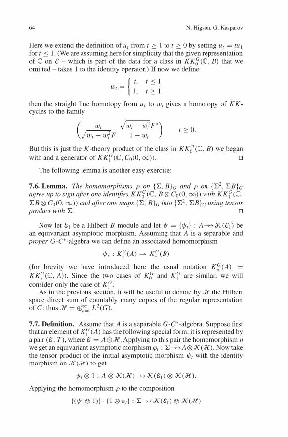
64 N. Higson, G. Kasparov
Here we extend the definition of ut from t ≥ 1 to t ≥ 0 by setting ut = tu1for t ≤ 1. (We are assuming here for simplicity that the given representationof C on E – which is part of the data for a class in KK G
0 (C, B) that weomitted – takes 1 to the identity operator.) If now we define
wt =
t, t ≤ 11, t ≥ 1
then the straight line homotopy from ut to wt gives a homotopy of KK -cycles to the family(
wt
√wt −w2
t F∗√wt −w2
t F 1−wt
)t ≥ 0.
But this is just the K -theory product of the class in KK G0 (C, B) we began
with and a generator of KK G1 (C,C0(0,∞)).
The following lemma is another easy exercise:
7.6. Lemma. The homomorphisms ρ on Σ, BG and ρ on Σ2,ΣBGagree up to sign after one identifies KK G
0 (C, B⊗C0(0,∞)) with KK G1 (C,
ΣB⊗C0(0,∞)) and after one maps Σ, BG into Σ2,ΣBG using tensorproduct with Σ.
Now let E1 be a Hilbert B-module and let ψ = ψt : A→→K(E1) bean equivariant asymptotic morphism. Assuming that A is a separable andproper G-C∗-algebra we can define an associated homomorphism
ψ∗ : K G∗ (A)→ K G
∗ (B)
(for brevity we have introduced here the usual notation K G∗ (A) =KK G∗ (C, A)). Since the two cases of K G
0 and K G1 are similar, we will
consider only the case of K G1 .
As in the previous section, it will be useful to denote by H the Hilbertspace direct sum of countably many copies of the regular representationof G: thus H = ⊕∞n=1L2(G).
7.7. Definition. Assume that A is a separable G-C∗-algebra. Suppose firstthat an element of K G
1 (A) has the following special form: it is represented bya pair (E, T ), where E = A⊗H . Applying to this pair the homomorphism ηwe get an equivariant asymptotic morphism ϕt : Σ→→A⊗K(H ). Now takethe tensor product of the initial asymptotic morphism ψt with the identitymorphism on K(H ) to get
ψt ⊗ 1 : A ⊗K(H )→→K(E1)⊗K(H ).
Applying the homomorphism ρ to the composition
(ψt ⊗ 1) · 1⊗ ϕt : Σ→→K(E1)⊗K(H )

KK-theory for groups which act properly on Hilbert space 65
we get an element of KK G0 (C, B⊗C0(0,∞)) ∼= K G
1 (B). Call it ψ∗(E, T ).Now assume that A is a proper G-C∗-algebra. Then according to the Equiv-ariant Stabilization Theorem (cf. [26], 2.9; [23], 5.3),
E ⊕ (A ⊗H ) % A⊗H,
so any element of K G1 (A) is represented by a pair (E, T ), where E = A⊗H .
This allows us to define the required homomorphism ψ∗ on the whole groupK G
1 (A).We will need below the following simple modification of this construc-
tion. Letψ = ψt : ΣA→→K(E1) be an equivariant asymptotic morphism.Then one can define an associated homomorphism ψ∗ : K G
1 (A)→ K G0 (B)
as the following composition:
KK G1 (C, A)
η−→ Σ, AG suspension−−−−−−−→
Σ2,ΣAG composition−−−−−−−→withψ
Σ2, BG ρ−→ KK G1 (C, B ⊗ C0(0,∞)).
The hypothesis that A is proper allows one to view Σ, AG as homotopyclasses of equivariant asymptotic morphisms from Σ to A ⊗ K(H ) (nonontrivial Hilbert modules E need be considered), and this allows us tocarry out the composition of asymptotic morphisms in the middle of thesequence above.
7.8. Theorem. Assume that A is a proper G-algebra. Let x ∈ K G1 (A), y ∈
KK G1 (A, B), and let ψ = η(y) an asymptotic morphism ΣA→→K(E1),
where E1 is a Hilbert B-module. Then the elements ψ∗(x) ∈ KK G1 (C, B ⊗
C0(0,∞)) and x ⊗A y ∈ KK G0 (C, B) are equal, up to sign, after the two
KK-groups are identified by Bott Periodicity.
Proof. To simplify notation we will assume that x is represented by anoperator R ∈ M(A) (i.e. the Hilbert module E is A itself and not A ⊗Has in Definition 7.7). This does not change the argument. Let y = (E1, T ),and assume in addition that the action of A on E1 is non-degenerate. (Thisis always possible – see [22], Lemma 2.8). It means that we can extend thehomomorphism A → L(E1) to M(A).
Again to simplify notation, let us denote by the same letter R the imageof the operator R ∈ M(A) in L(E1). Set P = (R+ 1)/2, Q = (T + 1)/2.Let ut and vt be the approximate units in A and K(E1) respectively usedin Definition 7.2 (for the cases of K G
1 (A) and KK G1 (A, B) respectively).
Then the product x ⊗A y ∈ K G∗ (B) can be written in the form MR + iNTwhere i = √−1 and M, N are the operators used in the definition ofthe KK -product (see [22], Theorem 2.11). The operators M and N areG-continuous operators with the following properties:

66 N. Higson, G. Kasparov
(i) M ≥ 0, N ≥ 0, and M2 + N2 = 1.(ii) M(P2−P), M(P∗−P), M(g(P)−P), g(M)−M, N[P, Q], N(Q2−Q),
N(Q∗ − Q), and N(g(Q)− Q) are elements of K(E1), for all g ∈ G.(iii) The functions g → M(g(P) − P) and g → N(g(Q) − Q) are norm-
continuous on G.
On the other hand, the composition η(y) · η(x) can be written as
Σ2→→ΣA→→K(E1) : f1 ⊗ f2 → f1(vs(t))Q f2(ut)P,
where we denote also by the same letter ut the image of ut in L(E1). Heres(t) denotes a reparametrization of the sort which is necessary in order todefine the composition of two asymptotic morphisms.
To compare ρ(η(y) · η(x)) with x ⊗A y ∈ K G∗ (B), we first changeη(y) ·η(x) by a certain homotopy. Namely, we replace f2(ut) by f2(1−M)using the homotopy: r(1 − M) + (1 − r)ut, 0 ≤ r ≤ 1. After that, wecan forget about the reparametrization s(t), and the composition of ourasymptotic morphisms takes the form
Σ2→→ΣA→→K(E1) : f1 ⊗ f2 → f1(vt) f2(1− M)PQ.
This latter asymptotic morphism has the form of η(z), where z ∈ K G0 (B)
is given by the operator F = (exp(2πi(1 − M))− 1)PQ + 1 ∈ L(E1). Inview of Lemma 7.5, it remains to prove that F and MR + iNT representthe same element in K G
0 (B).Put X = MP, Y = NQ. These two operators commute modulo
K(E1). It follows from the properties of the operators M, N listed abovethat XY(X2 + Y 2 − 1) ∈ K(E1). This means that the map C([0, 1]2) →L(E1)/K(E1) given by the formula: f → f(X,Y ) factors through the quo-tient algebra C([0, 1]2)/J , where J is the ideal generated by xy(x2+ y2−1).The quotient is the algebra of continuous functions on the contour whichbounds that quarter of the unit circle which lies in the first quadrant of the(x, y)-plane.
First, we will find operators homotopic to MR + iNT and F which arefunctions of X,Y . We have: MR+ iNT = 2(X + iY )− (M+ iN). We canmultiply the latter operator by M − iN (which is homotopic to 1) and get:
(M−iN)(2X+2iY )−1 = 2X2+2Y 2−2iX(1−X2)1/2+2iY(1−Y 2)1/2−1
modulo K(E1). For the operator F we find:
(exp(−2πiM)− 1)PQ + 1 = (exp(−2πiX)− 1)(1− X2)−1Y 2 + 1
modulo K(E1). Now it remains to note that the two maps from our quarter-circle contour to the unit circle given by the formulas:
(x, y) → 2x2 + 2y2 − 2ix(1 − x2)1/2 + 2iy(1− y2)1/2 − 1
and(x, y) → (exp(−2πix)− 1)(1− x2)−1 y2 + 1
are homotopic. This is done by checking that the winding numbers are thesame; the simple calculation is omitted.
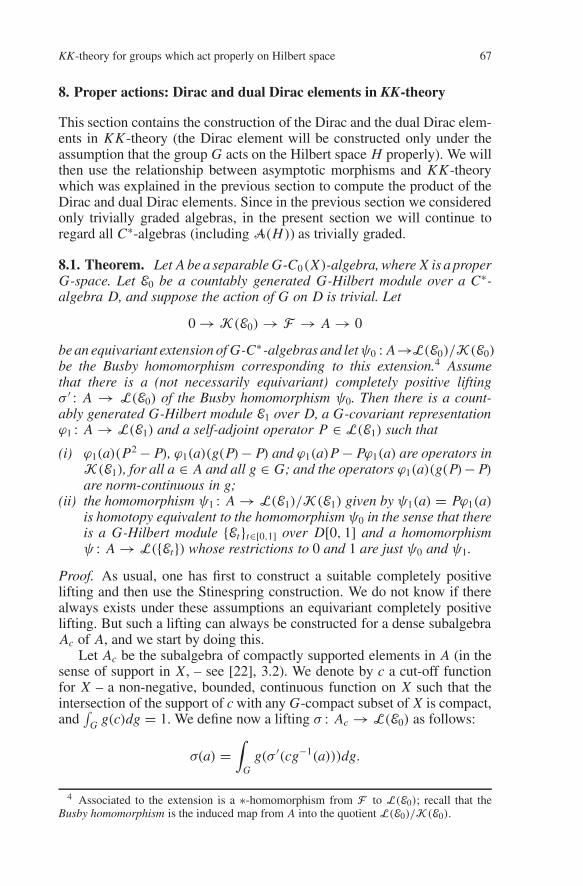
KK-theory for groups which act properly on Hilbert space 67
8. Proper actions: Dirac and dual Dirac elements in KK-theory
This section contains the construction of the Dirac and the dual Dirac elem-ents in KK -theory (the Dirac element will be constructed only under theassumption that the group G acts on the Hilbert space H properly). We willthen use the relationship between asymptotic morphisms and KK -theorywhich was explained in the previous section to compute the product of theDirac and dual Dirac elements. Since in the previous section we consideredonly trivially graded algebras, in the present section we will continue toregard all C∗-algebras (including A(H)) as trivially graded.
8.1. Theorem. Let A be a separable G-C0(X)-algebra, where X is a properG-space. Let E0 be a countably generated G-Hilbert module over a C∗-algebra D, and suppose the action of G on D is trivial. Let
0 →K(E0)→ F → A → 0
be an equivariant extension of G-C∗-algebras and letψ0 : A→L(E0)/K(E0)be the Busby homomorphism corresponding to this extension.4 Assumethat there is a (not necessarily equivariant) completely positive liftingσ ′ : A → L(E0) of the Busby homomorphism ψ0. Then there is a count-ably generated G-Hilbert module E1 over D, a G-covariant representationϕ1 : A → L(E1) and a self-adjoint operator P ∈ L(E1) such that
(i) ϕ1(a)(P2− P), ϕ1(a)(g(P)− P) and ϕ1(a)P− Pϕ1(a) are operators inK(E1), for all a ∈ A and all g ∈ G; and the operators ϕ1(a)(g(P)− P)are norm-continuous in g;
(ii) the homomorphism ψ1 : A → L(E1)/K(E1) given by ψ1(a) = Pϕ1(a)is homotopy equivalent to the homomorphism ψ0 in the sense that thereis a G-Hilbert module Ett∈[0,1] over D[0, 1] and a homomorphismψ : A → L(Et) whose restrictions to 0 and 1 are just ψ0 and ψ1.
Proof. As usual, one has first to construct a suitable completely positivelifting and then use the Stinespring construction. We do not know if therealways exists under these assumptions an equivariant completely positivelifting. But such a lifting can always be constructed for a dense subalgebraAc of A, and we start by doing this.
Let Ac be the subalgebra of compactly supported elements in A (in thesense of support in X, – see [22], 3.2). We denote by c a cut-off functionfor X – a non-negative, bounded, continuous function on X such that theintersection of the support of c with any G-compact subset of X is compact,and
∫G g(c)dg = 1. We define now a lifting σ : Ac → L(E0) as follows:
σ(a) =∫
Gg(σ ′(cg−1(a)))dg.
4 Associated to the extension is a ∗-homomorphism from F to L(E0); recall that theBusby homomorphism is the induced map from A into the quotient L(E0)/K(E0).

68 N. Higson, G. Kasparov
Note that the integral converges for any compactly supported a because theintegrand vanishes off a compact subset of G. The map σ is an equivariantlifting of ψ0 on Ac and it is completely positive in a suitable sense (seebelow). However, it may be unbounded and so it cannot be used directly inthe Stinespring construction.
Denote by Gd the group G equipped with the discrete topology anddenote by Balg the algebraic crossed product of Gd and Ac . Thus the elementsof Balg are finite sums
∑i ai gi where ai ∈ Ac, gi ∈ G; the product is given
by a1g1 · a2g2 = a1g1(a2)g1g2; the involution by (ag)∗ = g−1(a∗)g−1. Weextend the map σ defined above to Balg in the obvious way: σ(ag) = σ(a)g.In this formula, the symbol g on the right denotes the unitary operator on E0implementing the action of the element g of the group Gd . It easy to checkthat the map σ so defined is completely positive in the sense that σ appliedto a matrix with entries ((ai gi)
∗(aj g j)) gives a positive matrix over L(E0).Denote by B the crossed product C∗-algebra C∗(Gd, A). Let B be the C∗-
algebra B with unit adjoined. If u ∈ Ac is self-adjoint then the formula b →ubu defines a completely positive map κu : Balg → Balg, and composing κuwith σ we get a completely positive map σκu : Balg → L(E0). Since Balgis a dense subalgebra in B, and since σκu is bounded in the norm of B, itextends to a continuous map that we will denote σu : B → L(E0).
Now we will apply an infinite inductive procedure borrowed fromLemma 3.1 and Theorem 6 of [1], and we will also make use of Remark 2.5of [8]. If ui is a quasicentral approximate unit in A consisting of elementsof Ac (the word “quasicentral” here means quasicentral with respect to theaction of G) then define unital completely positive maps σi : B → L(E0)by the formula
σi(b) = u−1/2i σui(b)u
−1/2i ,
where b ∈ B and ui = sup(1, σ(ui)). It is clear that ψ(σi(b)) = u1/2i bu1/2
i
for every b ∈ B. Our general aim is to modify the maps σi : B → L(E0) soas to obtain a sequence of unital completely positive maps σi : B → L(E0)which converge pointwise to a completely positive map σ that is properlysuited to a subsequent Stinespring construction. First we will give the generalform of the modification procedure. Then by making appropriate choices ofapproximate units we will prove convergence of the modified maps.
Let vi be an approximate unit in K(E0) which is quasicentral withrespect to the algebra F and the action of G, and define unital maps σi : B →L(E0) inductively by setting σ1 = σ1 and then defining
σn(b) = v1/2n σn−1(b)v
1/2n + (1− vn)
1/2σn(b)(1− vn)1/2
for b ∈ B. Notice that
‖σn(b)− σn−1(b)‖ ≤∥∥v1/2
n σn−1(b)v1/2n − σn−1(b)vn
∥∥+ ∥∥(1− vn)
1/2σn(b)(1− vn)1/2 − σn(b)(1− vn)
∥∥+ ‖(σn(b)− σn−1(b))(1− vn)‖.

KK-theory for groups which act properly on Hilbert space 69
So in order to prove pointwise convergence we make the following choicesof the approximate units vi and ui. Let X be a compact subset of Awhose linear span is dense in A. Also let K1 ⊂ K2 ⊂ ... be an exhaustivefamily of compact subsets of G. Choose (in an inductive fashion) vn so thatwhen b belongs to the set ∑m am gm | am ∈ X, gm ∈ Kn the first twosummands on the right side of the above inequality are small. Concerningthe third summand, we know at least that for b ∈ B,
ψ(σn(b)− σn−1(b)) = u1/2n bu1/2
n − u1/2n−1bu1/2
n−1.
The norm of this element is small (for all b belonging to the same set asabove) if the approximate unit ui is chosen appropriately. Finally, notethat for any f ∈ F , the norms ‖ f(1− vn)‖ converge to ‖ψ( f )‖ as n goesto infinity. So the third summand on the right hand side of our inequalitywill also be small if vn has been chosen appropriately.
We have constructed a pointwise convergent sequence of completelypositive unital maps σn : B → L(E0). Denote the limit by σ : B → L(E0).The map σ possesses an important property which easily follows from theconstruction given above:
(∗) for any b ∈ B, the functions g → σ(bg) − σ (b)g and g → σ (gb) −gσ(b) are norm-continuous on G.
This completes the first part of the proof: the construction of a unital com-pletely positive lifting.
Consider now the algebraic tensor product B⊗C E0. Using the completelypositive map σ : B → L(E0), define a D-inner product on B ⊗C E0 by
(b1 ⊗ x1, b2 ⊗ x2) = (x1, σ (b∗1b2)x2).
By applying the argument given in the proof of the Stinespring Theorem(Theorem 3) of [19] we obtain a Hilbert module E over D and a repre-sentation ϕ : B → L(E ) (the representation ϕ comes from the action ofB on B ⊗ E0 defined by left multiplication). Our initial Hilbert module E0
is a direct summand of E , and the compression of ϕ : B → L(E ) to E0
is σ . We denote the orthogonal projection of E onto E0 by Q0. Since thecompression of ϕ : B → L(E ) to E0 is multiplicative modulo K(E0), it iseasy to deduce (see, for instance, the proof of Lemma 1 of Sect. 7 in [20])that Q0 commutes modulo K(E ) with ϕ(B).
Unfortunately, the Hilbert module E will not serve as the Hilbert moduleE1 in the statement of the theorem we are trying to prove because there maybe no G-action on E (the G-action corresponding to the homomorphism ϕmay be degenerate). A well defined G-action exists only on a submoduleB · E % B ⊗B E of E which we will call E1. This G-action comes from theaction of G on B by left multiplication. It is easy to check using property(∗) above and the definition of the inner product on E1 that this G-actionis continuous. The continuity of the G-action together with the separability

70 N. Higson, G. Kasparov
of the algebra A imply that E1 is countably generated. We denote by ϕ1 thehomomorphism A → L(E1) defined by the action of A on E1 given by leftmultiplication.
Now we have to construct the operator P ∈ L(E1). For this we note thatthe C∗-algebra B has a countable approximate unit (namely the approximateunit ui that was already used above), so by the Stabilization Theorem(Theorem 2 of [19]) the Hilbert B-module B is a direct summand of B⊗2.This means that the Hilbert D-module E1 = B ⊗B E is a direct summandof (B⊗ 2)⊗B E % E ⊗ 2. We denote by Q1 ∈ L(E ⊗ 2) the orthogonalprojection onto E1 and define P ∈ L(E1) as the compression Q1(Q0⊗1)Q1
of Q0 ⊗ 1 ∈ L(E ⊗ 2) to E1.In order to check condition (i) in the statement of the Theorem, we note
that although the projections Q0⊗ 1 and Q1 ∈ L(E ⊗ 2) do not commute,one has for any b ∈ B, (ϕ⊗1)(b) · [Q1, Q0⊗1] ∈ K(E⊗2). This easilyimplies all assertions of condition (i) except the last one: norm-continuity.However, as was pointed out in [28] (see the remark made after the proof ofTheorem 1.1.4), the norm-continuity of operators ϕ1(a)(g(P)− P) followsfrom the other assertions of condition (i). (One has to apply Theorem 1.1.4of [28] to the natural extension of C∗-algebras defined by the Busby homo-morphism ψ1 of condition (ii) in the statement of our Theorem 8.1.)
Coming finally to the last assertion (condition (ii)) of the theorem, we firstpoint out that there is a natural homotopy of Hilbert B-modules joining Band B. This is given by Z(B, B) = f : [0, 1] → B | f((1) ∈ B. Using theStabilization Theorem, we get a homotopy of projections in L(B[0, 1]⊗2)
whose image is just the above homotopy of Hilbert modules Z(B, B). Taking⊗B[0,1]E , we get a homotopy of projections St ∈ L(E[0, 1] ⊗ 2) joininga coordinate projection of E⊗2 onto a direct summand E with the projectionQ1 onto E1. Now consider the compression Pt = (Q0 ⊗ 1)St(Q0 ⊗ 1) ∈L(E0 ⊗ 2) of this homotopy of projections.
Note that the homomorphism ϕ⊗ 1 : A → L(E ⊗ 2), after being com-pressed first by the projection Q0⊗1 and then multiplied by the homotopy ofoperators Pt , becomes a homotopy of homomorphisms of A into the Calkinalgebra of the Hilbert module E0 ⊗ 2. At the point t = 0 we obtain thehomomorphism ψ0⊕0 and at the point t = 1 we obtain the homomorphismψ1 ⊕ 0. The assertion in condition (ii) follows.
We can define now the Dirac and the dual Dirac elements in KK -theory.For the construction of the Dirac element we will have to assume that theaction of the group G on the Hilbert space H is proper. The constructionof the dual Dirac element does not require this assumption. The propernessof G-action on H implies that the G − C∗-algebra A(H) is proper (Propo-sition 4.9). Also this algebra is nuclear as the inductive limit of nuclearalgebras. This means that the extension of C∗-algebras
0 →K(S⊗E )→ Fh(H)→ A(H)→ 0
described before Definition 6.7 admits a completely positive cross-section.

KK-theory for groups which act properly on Hilbert space 71
8.2. Definition. Let the action of G on H be proper. Denote by d the elem-ent of KK G
1 (A(H),SΣ) % KK G1 (A(H),C) defined by the pair (E1, P)
constructed by means of Theorem 8.1 for the extension 0 → K(S⊗E )→Fh(H)→ A(H)→ 0. Also denote by d the restriction of this element toA(H). Call these elements the Dirac elements.
To define suitable dual Dirac elements we use the ∗-homomorphismfrom A(0) into A(H) which is associated to the inclusion of the zerosubspace into H . Using the functional calculus, this map may be presentedin the form f → f(B), where B is a uniquely determined unboundedmultiplier of A(H), which we shall call the unbounded Bott element forA(H). There is a similar element for A(H). Compare Definition 4.4, whichgives concrete formulas for these Bott elements in finite dimensions.
8.3. Definition. Let B be the unbounded Bott element for the algebraA(H). Denote by b the element of KK G
1 (C, A(H)) defined by the operatorB(1+B2)−1/2 ∈M(A(H)), and denote by b the image of this element inKK G
1 (C,A(H)). (The element b is defined by the operatorB(1+B2)−1/2 ∈M(A(H)) whereB is the unbounded Bott element for the algebra A(H).)Call these elements the dual Dirac elements.
8.4. Lemma. The Dirac element d in KK-theory and the Dirac asymp-totic morphism α of Definition 6.7 are related by the equalities: η(d) = α,η(d) = α, where η is the homomorphism of Definition 7.2. The dual Diracelement in KK-theory and the dual Dirac asymptotic morphism of Defin-ition 6.6 are related by the equalities: η(b) = β, η(b) = β.
Proof. Only the equalities for the dual Dirac elements require proof. Thecalculation in this case is a standard one, and proceeds as follows. Let uswrite
Pt = 2t−1B(1+ t−2
B2)−1/2 − 1.
Then η(b) is represented by the asymptotic morphism C0(0, 1) → A(H)defined by the formula
f → f(ut)P1.
Here ut is a suitable quasicentral approximate unit, as in Definition 7.2.On the other hand the dual Dirac asymptotic morphism C0(R)→ A(H) isgiven by the formula
h → h(t−1B).
If we identify (0, 1) and R via the correspondence x ↔ 2x(1+ x2)−1/2− 1then the dual Dirac asymptotic morphism becomes the asymptotic morphismC0(0, 1)→ A(H) given by the formula
f → f(Pt).

72 N. Higson, G. Kasparov
To show that this is homotopic to the asymptotic morphism f → f(ut)P1 wefirst note that for f ∈ C0(0, 1) the families f(ut)P1 and f((1−ut)
1/2 P1(1−ut)
1/2) are asymptotic to one another. Indeed both families determine asymp-totic morphisms on C0[0, 1) and they agree (up to asymptotic equivalence)on the generating function f(x) = 1−x. Next, as long as s(t) is a sufficientlyslowly growing function of t the families f((1 − ut)
1/2 P1(1 − ut)1/2) and
f((1−ut)1/2 Ps(t)(1−ut)
1/2) are asymptotic. Finally, connecting ut to 0 by thestraight line homotopy gives a homotopy from f((1−ut)
1/2 Ps(t)(1−ut)1/2)
to f(Ps(t)). A reparametrization now completes the proof. 8.5. Theorem. Assume that the action of G on H is proper. Then b⊗A(H )d= 1 ∈ KK G(C,C) and b⊗A(H ) d = 1 ∈ KK G(C,C).
Proof. In view of the previous Lemma, the assertion follows from Theo-rems 6.10, 7.8 and Lemma 7.5.
One can also calculate the product of the Dirac and the dual Diracelements in the reverse order. This calculation is not used in the proof of themain results of this paper. It is based on Theorem 6.11 and the isomorphismof equivariant E and KK -theories in the case when the first argument isa proper algebra (see [23]). We omit the proof but give only the statementof this result.
8.6. Theorem. Assume that the action of G on H is proper. Then d⊗C b =1A(H ) ∈ KK G(A(H),A(H))and d⊗C b = 1A(H ) ∈ KK G(A(H), A(H)).
9. Consequences
9.1. Theorem. Any locally compact group G acting properly, isometricallyon a Hilbert space satisfies the Baum-Connes conjecture with coefficientsin any separable G-algebra.
Proof. The assertion follows from Proposition 4.9, Theorem 8.5 and Theo-rem 7.1.
This theorem has the following corollary:
9.2. Corollary. All second-countable locally compact amenable groupssatisfy the Baum-Connes conjecture with coefficients.
Proof. It is proved in [4] that any countable amenable group acts properly,isometrically on a Hilbert space. It is a simple matter to extend the argumentof [4] to second-countable locally compact amenable groups.
The following result which was first proved in [17] can now be obtainedfrom Theorem 8.5. It is interesting to point out that unlike [17], we deducethis result here without using representation theory of Lie groups at all.We recall from [22], 5.7, that for any Lie group G there exists a canonicalidempotent element γG in the ring KK G(C,C).
KK-theory for groups which act properly on Hilbert space 73
9.3. Theorem. The element γG ∈ KK G(C,C) for the group G = SU(n, 1)is equal to 1.
Proof. The following characterization (or rather definition) of the elementγG for a locally compact group G appeared as a remark in one of theearliest versions of [23]. It has become part of folklore now.5 The elementγG ∈ KK G(C,C), when it exists for a locally compact group G, is uniquelycharacterized by the following two properties:
1. γG = x ⊗A y, where x ∈ K G∗ (A), y ∈ K∗G(A) for some proper
G − C∗-algebra A.2. p∗(γG ) = 1 in RKK G(EG; C,C), where p is the map of EG to a point.
The proof of uniqueness is a simple exercise. In our case we take A = A(H),x = b, and y = d.
Finally it also follows from Proposition 4.9, Theorem 8.5 and Theo-rem 7.1 that:
9.4. Theorem. Any locally compact group acting properly, isometricallyon a Hilbert space is K-amenable.
References
1. W. Arveson, Notes on extensions of C∗-algebras, Duke Math. J. 44 (1977), 329–3552. M.F. Atiyah, Bott periodicity and the index of elliptic operators, Oxford Quarterly J.
Math. 19 (1968), 113–1403. P. Baum, A. Connes, N. Higson, Classifying space for proper actions and K -theory of
group C∗-algebras, Contemp. Math. 167 (1994), 241–2914. M.E.B. Bekka, P.-A. Cherix, A. Valette, Proper affine isometric actions of amenable
groups, in: Novikov conjectures, Index theorems and rigidity, Vol. 1, S. Ferry, A. Ran-icki, J. Rosenberg, editors, Cambridge University Press, Cambridge 1995, pp. 1–4
5. J. Chabert, S. Echterhoff, R. Meyer, Deux remarques sur l’application de Baum-Connes,preprint, 2000
6. A. Connes, N. Higson, Deformations, morphismes asymptotiques et K -theorie bivari-ante, C.R. Acad. Sci. Paris 311, Serie 1 (1990), 101–106
7. J. Cuntz, K -theoretic amenability for discrete groups, J. Reine Angew. Math. 344(1983), 180–195
8. J. Cuntz, G. Skandalis, Mapping cones and exact sequences in KK -theory, J. OperatorTheory 15 (1986), 163–180
9. S. Ferry, A. Ranicki, J. Rosenberg, A history and survey of the Novikov conjecture,in: Novikov conjectures, Index theorems and rigidity, Vol. 1, S. Ferry, A. Ranicki,J. Rosenberg, editors, Cambridge University Press, Cambridge, 1995, pp. 7–66
10. M. Gromov, Asymptotic invariants of infinite groups, in: Geometric group theory,G.A. Niblo, M.A. Roller, editors, Cambridge Univeristy Press, Cambrige, 1993, pp. 1–295
11. E. Guentner, N. Higson, J. Trout, Equivariant E-theory, Memoir Amer. Math. Soc., toappear
12. U. Haagerup, An example of a non-nuclear C∗-algebra which has metric approximationproperty, Invent. math. 50 (1979), 279–293
5 The reader is warned that a slightly different definition is used in [11].
74 N. Higson, G. Kasparov
13. P. de la Harpe, A. Valette, La propriete (T) de Kazhdan pour les groupes localementcompacts, Asterisque 175, Soc. Math. de France 1989
14. N. Higson, G. Kasparov, Operator K -theory for groups which act properly and isomet-rically on Hilbert space, E.R.A. Amer. Math. Soc. 3 (1997), 131–142
15. N. Higson, G. Kasparov, J. Trout, A Bott periodicity theorem for infinite dimensionalEuclidean space, Advances in Math. 135 (1998), 1–40
16. P. Julg, Travaux de N. Higson and G. Kasparov sur la conjecture de Baum-Connes,Seminaire Bourbaki 841 (1997–98)
17. P. Julg, G. Kasparov, Operator K -theory for the group SU(n,1), J. Reine Angew. Math.463 (1995), 99–152
18. P. Julg, A. Valette, K -theoretic amenability for SL2(Q p ), and the action on the associ-ated tree, J. Functional Analysis 58 (1984), 194–215
19. G.G. Kasparov, Hilbert C∗-modules: Theorems of Stinespring and Voiculescu, J. Op-erator Theory 4 (1980), 133–150
20. G.G. Kasparov, The operator K -functor and extensions of C∗-algebras, Math. USSRIzv. 16 (1981), 513–572
21. G.G. Kasparov, Lorentz groups: K -theory of unitary representations and crossed prod-ucts, (English Transl.), Sov. Math. Dokl. 29 (1984), 256–260
22. G.G. Kasparov, Equivariant KK -theory and the Novikov conjecture, Invent. math. 91(1988), 147–201
23. G. Kasparov, G. Skandalis, Groups acting properly on “bolic” spaces and the Novikovconjecture, preprint 1998, revised 1999
24. E. Kirchberg, S. Wassermann, Operations on continuous bundles of C∗-algebras, Math.Ann. 303 (1995), 677–697
25. E. Kirchberg, S. Wassermann, Exact groups and continuous bundles of C∗-algebras,Math. Ann. 315 (1999), 169–203
26. N.C. Phillips, Equivariant K -theory for proper actions, Longman Scientific & Technical1989
27. J. Rosenberg, S. Stolz, A ‘stable’ version of the Gromov-Lawson conjecture, Contemp.Math. 181 (1995), 405–418
28. K. Thomsen, Asymptotic equivariant E-theory I, preprint 199729. J.-L. Tu, The Baum-Connes conjecture and discrete group actions on trees, K-theory
17 (1999), 303–31830. J.-L. Tu, La conjecture de Baum-Connes pour les feuilletages moyennables, K-theory
17 (1999), 215–26431. S. Weinberger, Aspects of the Novikov conjecture, Contemporary Math. 105 (1990),
281–297