e shimbori 1004 - mri-jma.go.jp · the jma-ratm (japan meteorological agency regional atmospheric...

89

Fig. E-1-1. Flowchart of the JMA-RATM calculation for radionuclides.

E. JMA-RATM1

E-1. Original and Preliminary RATM

E-1-1. Description of RATM

The JMA-RATM (Japan Meteorological Agency Regional Atmospheric Transport Model, called

the ‘RATM’ in this chapter) is a mesoscale tracer transport model, which can be driven by the

JMA-MESO analysis GPVs (grid point values). The model takes a Lagrangian scheme (Iwasaki et al.,

1998; Seino et al., 2004) with many computational particles that follow advection, horizontal and

vertical diffusion, gravitational settling, wet scavenging and dry deposition processes. The RATM was

originally developed at JMA for photochemical oxidant predictions (Takano et al., 2007) and

volcanic-ash fall forecasts (Shimbori et al., 2009). In this section, we describe the original version of

RATM (Shimbori et al., 2010) and a preliminary version of RATM to simulate radionuclides for the

WMO technical Task Team (Saito et al., 2015). Flowchart of the RATM calculation for radionuclides

is shown in Fig. E-1-1. Specifications of each version of the RATM are summarized in Table E-1-1.

a. Advection

We write the position , , for each computational particle at time . The time

evolution after the time step ∆ is given by

∆ ∆ ∆ (E-1-1a)

∆ ∆ ∆ (E-1-1b)

∆ ∆ 2 ∆ Γ ∆ (E-1-1c)

with the mean wind velocity , , . On the right-hand sides of above equations, the

second and third terms represent advection and diffusion, respectively. The forth term of Eq. (E-1-1c)

represents gravitational settling.

1 T. Shimbori and K. Saito

Initial condition

Meteorological fields Time evolution

MESO analysesPrecipitation data

MESO or RAP data

Multiplier Outputs

Emission rate anddecay factor

Unit release at FDNPP

JMA-RATM

Calculation for the air concentration andsurface deposition

TECHNICAL REPORTS OF THE METEOROLOGICAL RESEARCH INSTITUTE No.76 2015

90

Table E-1-1. Specifications of JMA-RATM.

Version Original Preliminary Revised

Test for JMA Volcanic Ash Fall Forecast1

for WMO Task Team for SCJ Working Group

Model type Lagrangian description

Input meteorological field Hourly outputs of MESO forecast GPVs

Three-hourly outputs of MESO analysis GPVs

Number of particles 100,000/10 min. 100,000/3 h 300,000/3 h Time step 3 min. 10 min. 5 min.

Advection Horizontal Forward difference with spherical triangle Vertical Not adjusted Spatially-average and terrain-following at lowest model level

Horizontal diffusion Gifford (1982, 1984) Vertical diffusion Louis et al. (1982)

Gravitational settling2

(grain-size distribution)

Vpar: Suzuki (1983) (log-normal with Dm=0.25 mm, σD=1.0)

Ngas: N/A Dgas: N/A Lpar: Stokes’ law with Cunningham correction (log-normal with Dm=1 μm, σD=1.0)

Wet scavenging2

Washout3 (below-cloud)

Vpar: Kitada (1994) with MESO forecast (liquid rain)

Ngas: N/A Dgas: N/A Lpar: Kitada (1994) with MESO analysis (liquid rain) or RAP data below 3000 m a.s.l.

Ngas: N/A Dgas: N/A Lpar: same as left except application height below 1500 m a.s.l.

Ngas: N/A Dgas: N/A Lpar: same as left except using MESO analysis (liquid rain, solid snow and graupel)

Rainout (in-cloud)

Vpar: N/A Ngas: N/A Dgas: Hertel et al. (1995) Lpar: N/A

Ngas: N/A Dgas: same as left Lpar: Hertel et al. (1995)

Dry-deposition2 Vpar: Vd=0.3 m s-1

(Shao, 2000)

Ngas: N/A Dgas: Vd=0.01 m s-1 (Draxler and Rolph, 2012) Lpar: Vd=0.001 m s-1 (Draxler and Rolph, 2012)

Reflection on the ground N/A Iwasaki et al. (1998) Radioactive decay N/A Half-lifetime Output grid size 5 km

References Shimbori et al. (2010) Draxler et al. (2013a), Saito et al. (2015) Takigawa et al. (2013), Saito et al. (2015), SCJ (2014)

Saito et al. (2015)

1 As of March 2011. JMA-RATM for volcanic ash was replaced on March 2013 (Shimbori et al., 2014). 2 The abbreviations Ngas, Dgas, Lpar and Vpar mean noble gas, depositing gas, light aerosol and volcanic-ash particle, respectively. 3 Below-scavenging coefficients Λw are listed in Table E-3-4.


91

b. Horizontal diffusion

Under the assumption of horizontally homogeneous turbulence, the – and -components of

subgrid-scale turbulent velocity in Eqs. (E-1-1a) and (E-1-1b) are given by Uliasz (1990):

Δ Δ 1 Δ Γ (E-1-2a)

Δ Δ 1 Δ Γ (E-1-2b)

with the initial conditions 0 Γ and 0 Γ. The and are the magnitudes of

turbulent horizontal velocities at the emission point and Γ is a normal random number with mean 0

and variance 1. is the Lagrangian autocorrelation function of the turbulent velocity represented by

⁄ (E-1-3)

with Lagrangian time scale . and are the standard deviations of and , respectively,

given by

(E-1-4)

with the horizontal diffusion coefficient for ≫ . Substituting Eqs. (E-1-3) and (E-1-4) into

(E-1-2a) and (E-1-2b), to the first order in Δ , we obtain the Langevin equation. Then the horizontal

diffusion scheme represented by Eqs. (E-1-2a) and (E-1-2b) is the analogue of Brownian motion

(Gifford, 1982, 1984).

For the three parameters in Eqs. (E-1-2a), (E-1-2b) - (E-1-4), we set as 0.253ms ，

5.0 10 s and 5.864 10 m s according to Kawai (2002).

c. Vertical diffusion

The vertical diffusion coefficient in the third term on the right-hand side of Eq. (E-1-1c) are

determined by Louis et al. (1982):

∂∂ v (E-1-5)

where is the mixing length in an analogy to the mean free path in molecular diffusion, is the

mean horizontal wind velocity, and v representing atmospheric stability is a function of flux


92

Richardson number given by the level 2 scheme of Mellor and Yamada (1974, 1982). The mixing

length takes the form (Blackadar, 1962)

z1 ⁄

(E-1-6)

where is the Kármán constant (≈0.4), is height from ground surface and is maximum mixing

length [m] given by Holtslag and Boville (1993):

30 70 exp 11000

, 1000 m

100 , 1000 m (E-1-7)

The upper limit of is set to 50 m2 s-1 according to Yamazawa et al. (1998).

The above-mentioned schemes of advection and diffusion are used in original RATM and are also

applied to radionuclides in the preliminary and revised RATM.

d. Gravitational settling

For dealing with light particles (Lpar) of radionuclides, i.e. radioactive matter or other

accumulation-mode aerosol particles carrying some radioactive matter (e.g. 137Cs), gravitational

settling follows Stokes’ law with a slip correction and the terminal velocity is given by (e.g., Sportisse,

2007)

,

118 ⁄

(E-1-8)

where is the Cunningham correction factor

1 exp , 1.257, 0.400, 1.100 (E-1-9)

with the Knudsen number ≡ 2 ⁄ . The viscosity and the mean free path of air are

calculated by

⁄

(E-1-10)

⁄

(E-1-11)


93

where a the air pressure, the air temperature, the Sutherland constant of air (=117 K) and

18.2 Pas , 0.0662 m are the standard values for the reference atmosphere (

293.15K, 1013.25hPa). The distribution of particle size is assumed to be log-normal with

mean diameter 1μm and standard deviation 1.0 (upper cutoff: 20 μm). The particle

density is 1 g cm-3 for all particle sizes.

Note that if a computational particle moves under the model surface by the vertical motion, it is

numerically reflected to the mirror symmetric point above the surface.

e. Wet scavenging

(1) Washout (below-cloud scavenging)

Because the original RATM was not applied in predicting the dispersion and deposition of

radionuclides, the wet scavenging schemes needed to be modified for this application. For Lpar, based

on the original treatment of wet scavenging, only washout processes (below-cloud scavenging) are

considered. The below-cloud scavenging rate by rain (liquid water) is given by Kitada (1994) (red

solid line of Fig. E-1-2):

Λ (E-1-12)

2.98 10 s , 0.75 (E-1-13)

where is the precipitation intensity [mm h-1].

(2) Rainout (in-cloud scavenging)

On the other hand, wet deposition for a depositing gas (Dgas, e.g. 131I) is considered only as a

rainout process (in-cloud scavenging). The in-cloud scavenging rate for Dgas is given by Hertel et al.

(1995):

Λ

11 ⁄

h (E-1-14)

where the liquid water content, the Henry constant (=0.08 M atm-1; Sect. F-1), the

ideal-gas constant (=0.082 atm M-1 K-1), and the height over which in-cloud scavenging takes

place.

Wet scavenging is applied to Lpar or Dgas under the height of about 3000 m a.s.l. in the original

and preliminary RATM (Shimbori et al. 2010). In the case of in-cloud scavenging for Dgas, however,

we have not been able to calibrate the RATM results. Therefore the Sect. E-3 results are devoted to

Lpar (137Cs and particulate 131I) verification.


94

f. Dry deposition

Dry deposition is simply computed from the following deposition rate (e.g., Iwasaki et al., 1998):

Λ (E-1-15)

where is the dry-deposition velocity and is the depth of surface layer. The value of is set

to 0.001 m s-1 for Lpar and 0.01 m s-1 for Dgas (Sportisse, 2007; Draxler and Rolph, 2012), and is

set to 100 m for both tracer types.

E-1-2. Use of MESO GPVs and RAP data

In Fig. E-1-1, the motion of computational particles in RATM is calculated in the same coordinate

system as the MESO analysis (Lambert conformal mapping in the horizontal and a terrain-following

hybrid in the vertical). The three-hourly 5-km MESO GPV data used to drive the RATM are

momentum, potential temperature, pressure, density, accumulated precipitation and mixing ratio of

cloud water. In the advection and diffusion steps, the mean wind velocities at each computational

particle are calculated from the time-space interpolation of the density and momentum GPVs. To

calculate the settling velocity, the temperature and pressure GPVs are used. For the wet scavenging

process, the precipitation intensity is computed from the average of the three-hour accumulated

precipitation GPVs. for the in-cloud scavenging computation can be defined by the GPVs of

mixing ratio of cloud water. However, due to limitations in the treatment of ice-phase deposition in the

original RATM, only liquid rain was considered in the WMO Task Team calculation. Subsequently,

we used the total precipitation in the SCJ (Science Council of Japan) Working Group calculations.

When using the RAP data, instead of the three-hourly accumulated precipitation by MESO GPVs,

the RAP intensity at each MESO grid point (5-km resolution) is calculated from the spatial average of

the surrounding 25-grid cells of RAP (1-km resolution) every 30 min. As noted above, because the

original version of RATM cannot treat ice-phase deposition and RAP data do not distinguish solid and

liquid precipitations, all RAP data were considered to be liquid rain in the calculation.

Fig. E-1-2. Below-cloud

scavenging coefficients for rain (red solid line) and snow and graupel (blue dotted line) used in JMA-RATM. After Saito et al. (2015).


95

E-2. Revision of RATM2

As previously mentioned in Sect. B-3-2, the JMA-MESO analysis is produced by a three-hour

forecast of the 5-km outer-loop of JMA-NHM (Saito et al., 2006, 2007, 2012) of JNoVA (Honda et al.,

2005; Honda and Sawada, 2008). The stored values in the analysis field are not averaged in the

assimilation window but are the instantaneous values predicted by the outer-loop model at the analysis

time (the end of each three-hour assimilation window). Because the instantaneous vertical motion is

affected by gravity waves and short-lived convection, a simple time interpolation of

updrafts/downdrafts between the three-hourly analysis fields may yield an overestimation of the

vertical advection of the air parcel, even if the magnitude of updrafts/downdrafts is small.

To compensate for the lack of temporal resolution, in the revised version of JMA-RATM, the

vertical advection (the second term on the right-hand side of Eq. (E-1-1c)) is calculated using a

spatially-averaged (nine-grid cells) value of the MESO vertical velocity and assumed to be

terrain-following ( ∗ 40m 0) at the lowest model level. Figure E-2-1 compares the 24-h

Lpar accumulated deposition for unit release (1 Bq/h) from 0000 UTC to 0300 UTC 14 March 2011.

The upper-right panel shows the result where vertical motion of the particles is computed using the

original MESO vertical velocity. Compared to the case without vertical advection (upper-left panel),

the deposition over the sea off the east coast of Japan is reduced. The lower-left panel provides the

result when the nine-grid cell averaged updraft/downdraft was applied to compute the vertical

advection. The difference from the upper-right panel is not large but the deposition is slightly

increased near the FDNPP (Fukushima Daiichi Nuclear Power Plant) site and slightly decreased at

distant areas. In these simulations, Lpar emitted from the FDNPP site were first lifted up by the lowest

level’s small updraft in MESO GPVs. The lower-right panel is the result of when the lowest level

vertical motion was assumed to be terrain following (i.e., the lowest level updraft/downdraft becomes

zero over sea while the remaining vertical motion over land is just due to the terrain slope and the

horizontal wind speed). The deposition off the east coast of Japan is increased.

In the preliminary version of RATM, wet scavenging was assumed to occur below about 3000 m in

height, the same as in the original RATM (Table E-1-1), but deposition over Miyagi prefecture, to the

north of Fukushima, was overestimated compared with the aircraft monitoring by the MEXT (Sect.

D-3). In the revised RATM, this overestimation was reduced by limiting the level of wet scavenging to

levels below about 1500 m (see Sect. E-3).

Some improper treatments of horizontal and vertical interpolations of the kinematic fields were

found in the preliminary version of RATM. These computational bugs were corrected in the revised

version. Also the number of computational particles was increased from 100,000/3 h to 300,000/3 h,

but the impact was almost negligible (see Sect. E-3).

For the model intercomparison of the SCJ Working Group, we further modified RATM as noted

previously: the time step was changed from 10 min. to 5 min. and in addition to rain, the precipitation

2 The description is based on Sect. 3 of Saito et al. (2015).


96

intensity of snow and graupel in the MESO GPVs was used. For these calculations, the below-cloud

scavenging coefficients of Lpar in Eq. (E-1-12) for snow and graupel are assumed (blue dotted line of

Fig. E-1-2)

2.98 10 s , 0.30 (E-2-1)

with reference to the value of UKMET-NAME (Table F-2-1). The impacts of the modifications are

shown in next section.

Fig. E-2-1. 24-h Lpar accumulated deposition by the JMA-RATM for unit release (1 Bq/h) at 0000-0300 UTC 14 March 2011. JMA-MESO GPV is used for precipitation. Upper left: without vertical advection. Upper right: vertical motion is computed by updraft/downdraft. Lower left: spatially-average is applied. Lower right: spatially-average and terrain-following at the lowest level. Star symbols indicate the location of FDNPP. These deposition maps are created by the drawing tool of the NOAA ARL website (Sect. D-4). After Saito et al. (2015).


97

E-3. Experiments with RATM3

E-3-1. Comparison with preliminary and revised RATM for the WMO Task Team

a. Experimental setting

According to the computational design described in Sect. D-1, JMA-RATM simulations were

conducted by the WMO Task Team for the computational period of 1800 UTC 11 March through

2400 UTC 31 March, in three-hourly emission period increments using a unit source rate (1 Bq/h) for

each discrete emission time segment. Emissions were uniformly distributed from the ground surface to

100 m a.g.l., and the concentration or deposition at any grid cell in the domain was given by the sum

of the contribution from all the RATM emission segments after multiplying the resulting unit

concentrations by the emission rate for each segment (Sect. D-1). The air concentration and deposition

output fields were configured to use a regular latitude-longitude grid (601 by 401 grid cells) with the

output averaged at three-hourly intervals at 0.05° (5 km) horizontal resolution and 100 m vertical

resolution. In the post-processing step, the results from each of the 168 RATM simulations were

multiplied by the actual emission rate at the release time of the simulation and decay constant for each

radionuclide thereby permitting the RATM dispersion and deposition factors to be applied to multiple

radionuclides. The estimated emission rates ‘JAEA’ (red solid line in Fig. 2 of Draxler et al. (2015)),

originally derived by Chino et al. (2011) and later modified by Terada et al. (2012, in Sect. D-2) were

used for the WMO Task Team simulations.

Figure E-3-1 compares 137Cs accumulated deposition for 11 March to 3 April 2011 estimated using

different computational methodologies. Here, rain in MESO GPVs was used for the calculations

shown in the left panels while RAP data were used for those shown in the right panels. In the

preliminary RATM (upper figures), deposition over Miyagi prefecture (north of Fukushima) and

southern part of the Kanto Plain (west of Tokyo) was overestimated compared with observation as

mentioned in the previous section E-2. In the revised RATM (lower figures), this overestimation was

ameliorated. When RAP data is used for precipitation, an area with high deposition in the northwest of

FDNPP becomes more distinctly reproduced (right figures), but the overestimation of deposition in the

southern part of the Kanto Plain is also enhanced, even in the revised RATM.

b. Verifications against observation

The 137Cs dispersion and deposition were verified against the observed time series of near ground

level air concentrations at JAEA-Tokai (see Sect. D-2) and the deposition measurements taken by

aerial and ground based sampling (Fig. D-3-1 in Sect. D-3). One of the characteristic features of the

deposition pattern is the densely contaminated area extending to northwest from FDNPP. This area is

bent to the south, east of Ou mountain range, and forms an inverse L-shaped pattern shown by the

yellow shaded region in Fig. D-3-1. On the other hand, deposition in Miyagi prefecture, north of

Fukushima, is relatively small.

3 The description is based on Sects. 4 and 5 of Saito et al. (2015).


98

Fig. E-3-1. 137Cs accumulated deposition for 11 March-3 April 2011 using the JAEA source. Upper left: preliminary RATM with MESO precipitation. Upper right: preliminary RATM with RAP precipitation. Lower: same as in upper panels but results by the revised RATM. After Saito et al. (2015).

The statistics of correlation coefficient ( 1 1 ), fractional bias ( 2 FB 2 ),

figure-of-merit in space (FMS % ), Kolmogorov-Smirnov parameter (KSP % ) mentioned in Sect.

D-3 and the following two additional statistics used in Draxler et al. (2013a) were applied to the

results of the preliminary and revised RATM.

i) Factor of two percentage (FA2 % ), the percentage of calculations within a factor of two of the

measured value.

ii) Factor of exceedance ( 50% FOEX 50%), the factor of the number of over-predictions in

the pairs of predicted and measured values.

A ranking method was defined by giving equal weight to the normalized expressions of these

statistics (Draxler et al., 2013a),

METRIC1 ≡ Rank 1

FB2

FMS100

1KSP100

(E-3-1a)

METRIC2 1

FB2

FA2100

1KSP100

(E-3-1b)


99

METRIC3 METRIC1 1

FOEX50

1

FB2

FMS100

1FOEX50

1KSP100

(E-3-1c)

METRIC4 METRIC3 2 100⁄

1

FB2

FMS100

FA2100

1FOEX50

1KSP100

(E-3-1d)

whose value would range from 0 to 4 (METRIC1 and 2), 5 (METRIC3), 6 (METRIC4) (from worst to

best). Eq. (E-3-1a) is same as the Rank defined in Sect. D-3.

Two sets of calculations were examined, one where the precipitation was given by the MESO GPVs

and the other using the RAP data. Table E-3-1 shows the verification statistics by RATM for 137Cs

deposition. Performance of the revised RATM (Rev. MESO) was significantly improved compared

with the preliminary RATM (Pre. MESO) for all rank metrics. The most improvement was obtained in

, which increased from 0.45 in the preliminary version to 0.70 in the revised version. The use of RAP

data for precipitation further improved the correlation coefficient to 0.84, while rank metrics became

slightly worse due to the deterioration of FB and FOEX. These tendencies in the statistics in the use

of RAP data can be understood by the area with high deposition in the northwest of FDNPP and the

overestimation of deposition in the west of the Kanto Plain in right panels of Fig. E-3-1; in the aircraft

monitoring by MEXT (Fig. 4 of Draxler et al. (2013a)), little or no deposition was observed in the

western part of the Kanto Plain.

Table E-3-2 and Fig. E-3-2 show the time evolution and the corresponding statistics for 137Cs

concentration at the JAEA-Tokai observation site. Performance of the revised RATM using MESO

precipitation was slightly improved in terms of the rank metrics, while the revision did not improve

the metrics when the RAP data were used for precipitation. The reason for this deterioration in metrics

in the use of RAP data is not obvious, but a similar tendency was also found in the other Task Team’s

model simulations (Chap. F). Arnold et al. (2015) inferred that the discrepancy of transport patterns by

NWP (numerical weather prediction) analyses and the locations of the precipitation may result in a

wrong description of the total wet scavenging. The quality of the RAP data itself is also arguable.

Table E-3-1. Statistical metrics for comparison of JMA-RATM simulations with observed deposition pattern of

137Cs using the JAEA source. Bold values indicate best score for each simulation. Reproduced from Saito et al. (2015).

RATM R FB FA2 (%)

FOEX(%)

FMS (%)

KSP(%)

METRIC 1

METRIC 2

METRIC 3

METRIC 4

Pre. MESO

0.45 -0.02 51.01 -0.46 100.00 10 3.09 2.60 4.08 4.59

Pre. RAP

0.77 0.54 41.99 9.67 100.00 11 3.22 2.63 4.02 4.44

Rev. MESO

0.70 -0.04 37.94 -0.83 99.63 10 3.37 2.75 4.35 4.73

Rev. RAP

0.84 0.56 35.73 9.12 99.08 13 3.28 2.65 4.10 4.46


100

Fig. E-3-2. Same layout as in Fig. E-3-1 but time evolution of 137Cs (logarithmic in the ordinate) at JAEA-Tokai for the period 13-31 March 2011. Black lines indicate observation. Red lines show results by the JMA-RATM with the JAEA source estimation. After Saito et al. (2015).

Table E-3-2. Statistical metrics for comparison of JMA-RATM simulations with observed concentration time series of 137Cs at JAEA-Tokai using the JAEA source. Bold values indicate best score for each simulation. Reproduced from Saito et al. (2015).

RATM R FB FA2 (%)

FOEX(%)

FMS(%)

KSP(%)

METRIC 1

METRIC 2

METRIC 3

METRIC 4

Pre. MESO

0.51 -0.82 21.43 -21.43 80.00 43 2.22 1.63 2.79 3.01

Pre. RAP

0.59 -1.66 4.76 -45.24 57.50 64 1.46 0.93 1.55 1.60

Rev. MESO

0.39 -0.40 14.29 -19.05 77.50 43 2.30 1.67 2.92 3.06

Rev. RAP

0.07 -1.68 9.52 -42.86 62.50 67 1.12 0.59 1.26 1.36


101

Table E-3-3. Statistical metrics for comparison of JMA-RATM simulations with observed concentration time series of particulate 131I at JAEA-Tokai using the JAEA source. Bold values indicate best score for each simulation. Reproduced from Draxler et al. (2013a).

RATM R FB FA2 (%)

FOEX(%)

FMS(%)

KSP(%)

METRIC 1

METRIC 2

METRIC 3

METRIC 4

Pre. MESO

0.47 -0.96 14.29 -30.95 78.05 43 2.09 1.45 2.47 2.62

Pre. RAP

0.67 -1.71 0.00 -45.24 60.98 60 1.60 0.99 1.70 1.70

Rev. MESO

0.14 -0.54 16.67 -23.81 75.61 40 2.11 1.52 2.63 2.80

Rev. RAP

0.02 -1.60 4.76 -42.86 60.98 65 1.16 0.60 1.30 1.35

Although the bright band is not likely critical in this experiment, radar echoes are scanned around the

level of 1 km a.g.l. and solid waters are over-detected in the radar reflectivity. A lower limit of

intensity around 0.4 mm h-1 is set in RAP, which means that very weak precipitation is not included.

As mentioned in Sect. E-1-1, all RAP precipitation was considered to be liquid rain in the wet

scavenging calculation in RATM, and this assumption also may yield some errors in the air

concentration time evolution. Another possibility is that dispersion of radionuclides to the position of

the JAEA site is somewhat uncertain. As suggested in Fig. C-9-7, the southward advection of

radionuclides from FDNPP on 15 March 2011 was sensitive to small changes in the wind direction.

Therefore, given the inherent limitations in the accuracy of wind direction in meteorological analyses,

it may be unrealistic to expect that an RATM can precisely reproduce the time evolution of downwind

air concentrations at JAEA-Tokai. In addition, the statistical results may also be affected by remaining

uncertainties in the radionuclides release rate estimates which may never be finalized.

Table E-3-3 shows the verification statistics for particulate 131I concentration at the JAEA-Tokai

observation site. Similar tendency of the RATM results were confirmed for another type of

radionuclides.

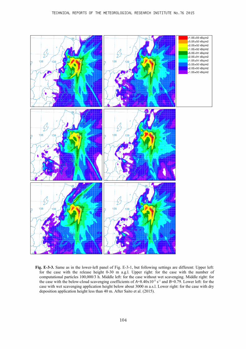
c. Sensitivity experiments to RATM parameters

In the revision of RATM, we tested some of the parameters with the greatest uncertainty to

determine their impacts on the RATM calculations of the accumulated deposition patterns of 137Cs

from 1800 UTC 11 March to 2100 UTC 03 April 2011. A list of values of parameters used in the

experiments and corresponding figures are given in Table E-3-4.

(1) Release height

In the WMO Task Teams’ experiments, emissions of radionuclides were assumed to be distributed

uniformly from the ground to 100 m a.g.l. But this release height may change depending on the

atmospheric conditions and situation of the emission. The upper-left panel of Fig. E-3-3 shows the 137Cs accumulated deposition when a lower release height of 30 m is applied. No significant difference

was obtained in the dense deposited area compared with the case of the original release height of 100

m (lower-left panel of Fig. E-3-1). A small difference can be seen in the regions with weak deposition


102

over southern part of the Kanto plain, where the simulated deposition becomes slightly smaller by

using the lower release height. This change corresponds to the observed deposition pattern (see Fig. 4

of Draxler et al. (2013a)), and small hotspot northeast of Tokyo is vaguely simulated in this

experiment.

(2) Number of computational particles

The upper-right panel of Fig. E-3-3 shows the result when a smaller number of computational

particles of 100,000/3 h were employed. Virtually the same result was obtained in the deposition

patterns.

(3) Wet scavenging coefficient and application height

Wet scavenging is an important process for the deposition of radionuclides. The middle-left panel of

Fig. E-3-3 indicates that when the wet scavenging process is not included in the simulation, the

deposition becomes much less compared with the original calculation (lower-left panel of Fig. E-3-1).

This result shows that the area with high deposition to the northwest of FDNPP was strongly affected

by wet scavenging. However the treatments of scavenging caused by rain and/or snow have many

ambiguities. The original version of RATM considered wet scavenging below 3000 m with the

scavenging coefficient of Eqs. (E-1-12) and (E-1-13). The middle-right panel of Fig. E-3-3 shows the

sensitivity of the results to changes in the below-cloud scavenging coefficient. Here, the scavenging

coefficients of Eq. (E-1-13) is replaced by 8.40 10 s , 0.79, the values used in

UKMET-NAME (Table F-2-1). When a lager value is applied, deposition of 137Cs over west of the

Kanto Plain is enhanced.

The lower-left panel of Fig. E-3-3 shows the result with the original scavenging application height

of 3000 m. A distinct difference from the original simulation is seen over Miyagi prefecture, where

overestimation of unobserved deposition is predicted. This result may suggest that the wet scavenging

should be confined in lower levels in the case of the FDNPP accident.

(4) Dry deposition application height

Sensitivities to dry deposition surface-layer height and number of computational particles were also

examined. Using a lower dry deposition surface layer height 40m (the lowest model layer) had

little impact on the deposition pattern (the lower-right panel of Fig. E-3-3).


103

Table E-3-4. List of values of parameters used in the JMA-RATM experiments and corresponding figures.

Source Release height (m a.g.l.)

Number of comp. particles (per 3 h)

Time step (min.)

Below-cloud scav. coeff. Scav. appl. height (m a.s.l.)

Dry-dep. appl. height (m a.g.l.)

Figures by rain by snow

JAEA 0-100 300,000 10 A=2.98x10-5,

B=0.75 N/A <1500 <100

low.-left of Fig. E-3-1

JAEA 0-30 300,000 10 A=2.98x10-5,

B=0.75 N/A <1500 <100

upp.-left of Fig. E-3-3

JAEA 0-100 100,000 10 A=2.98x10-5,

B=0.75 N/A <1500 <100

upp.-right of Fig. E-3-3

JAEA 0-100 300,000 10 N/A N/A N/A <100 mid.-left of Fig. E-3-3

JAEA 0-100 300,000 10 A=8.40x10-5,

B=0.79 N/A <1500 <100

mid.-right of Fig. E-3-3

JAEA 0-100 300,000 10 A=2.98x10-5,

B=0.75 N/A <3000 <100

low.-left of Fig. E-3-3

JAEA 0-100 300,000 10 A=2.98x10-5,

B=0.75 N/A <1500 <40

low.-right of Fig. E-3-3

JAEA2 0-100 300,000 10 A=2.98x10-5,

B=0.75 N/A <1500 <100

low.-left ofFig. E-3-4

JAEA2 0-100 300,000 5 A=2.98x10-5,

B=0.75 A=2.98x10-5,

B=0.30 <1500 <100

low.-right ofFig. E-3-4


104

Fig. E-3-3. Same as in the lower-left panel of Fig. E-3-1, but following settings are different: Upper left: for the case with the release height 0-30 m a.g.l. Upper right: for the case with the number of computational particles 100,000/3 h. Middle left: for the case without wet scavenging. Middle right: for the case with the below-cloud scavenging coefficients of A=8.40x10-5 s-1 and B=0.79. Lower left: for the case with wet scavenging application height below about 3000 m a.s.l. Lower right: for the case with dry deposition application height less than 40 m. After Saito et al. (2015).


105

Fig. E-3-4. Upper: distribution of 137Cs deposition by JMA-RATM in the SCJ model intercomparison. Lower left: Same as in the lower-left panel of Fig. E-3-1 (below-cloud scavenging is applied only to rain) but for the case that the release rate is given by JAEA2. Lower right: same as in the upper panel but an enlarged view for the same domain as in the lower-left panel of Fig. E-3-1. After Saito et al. (2015).

E-3-2. Results of revised RATM for the SCJ Working Group

The SCJ (2014) reviewed the modeling capability of the transport, dispersion and deposition of

radioactive materials released to the environment as a result of the FDNPP accident. The primary

purpose of this initiative was to assess the uncertainties in the simulation results through model

intercomparisons (Sect. G-6). In participating in these model intercomparisons, we used the revised

release rate ‘JAEA2’ by Kobayashi et al. (2013) and further modified RATM as mentioned at the end

of Sect. E-2.


106

Fig. E-3-5. Same as in the

lower-right panel of Fig. E-3-4 but for a test version of JMA-RATM that in-cloud scavenging for Lpar is considered. After Saito et al. (2015).

Figure E-3-4 shows the 137Cs deposition distribution obtained by the SCJ experiment. As seen in its

enlarged view (lower-right panel), the area with high deposition northwest of FDNPP is more

enhanced relative to the previous RATM results and linked with the hotspot at Naka-dori valley,

producing an inverse L-shaped pattern. Because the JAEA2 release rate is somewhat larger than that

of JAEA (Fig. 4 of Kobayashi et al. (2013)), the enhancement of deposition was partly caused by the

change of the release rate, while the modification of treatment of the wet scavenging (use of solid

waters in MESO GPVs) likely contributed to modifying the shape of the area with high deposition. It

is noteworthy that in this experiment, a small hotspot in Chiba prefecture (northeast of Tokyo, see Fig.

4 of Draxler et al. (2013a)) is better simulated compared with the previous RATM simulation (the

lower-left panel of Fig. E-3-1).

To differentiate the impact of changes to the emission rate and model, we conducted additional

experiments. The lower-left panel of Fig. E-3-4 is for the case when only the release rate is changed to

JAEA2 source term and with application of below-cloud scavenging only to rain (the same model that

in the lower-left panel of Fig. E-3-1). As indicated by these figures, both changes contribute to

enhance the inverse L-shaped area with high deposition, but the change of the source term has a larger

effect than inclusion of snow in the below-cloud scavenging in terms of the deposition distribution

over the Kanto Plain.

E-3-3. Test version of RATM for in-cloud scavenging and future research

Another experiment with in-cloud scavenging for Lpar was conducted to test its impact. In this

experiment, the three-dimensional distribution of cloud water analyzed by JNoVA was used to define

cloud area and liquid water content. In an analogous form to Eq. (E-1-14), the in-cloud scavenging

rate for Lpar is also given by Hertel et al. (1995):

Λ

0.9 h (E-3-2)


107

Figure E-3-5 shows the result when in-cloud scavenging of Eq. (E-3-2) is considered. A very large

difference is seen in the north of Kanto Plain. An area with high deposition extends from the eastern

part of Fukushima prefecture to west-southwest, resembling the observed hotspot in the northern

Kanto Plain (Fig. 4 of Draxler et al. (2013a)). Although the simulated area with high deposition has a

small (20-30 km) southward positional lag, this result suggests importance of considering in-cloud

scavenging for Lpar.

In the WMO Task Team and the SCJ Working Group experiments, we used three-hourly MESO

analysis as the meteorological field with linear interpolation in time and space to obtain input data for

RATM at every 5 or 10 min. time step. The time interval of the meteorological field may not be

sufficient to properly treat the upward motion of the radionuclides and to characterize their finer

spatiotemporal scale transport due to changes of the wind speed and direction. To obtain more

temporally resolved meteorological fields, additional mesoscale model simulations are needed. On the

progress of this subject, Sekiyama et al. (2015) conducted the RATM experiments (the same version

for SCJ Working Group) using the one-hourly 15 km, 3 km and 500 m NHM-LETKF GPVs (see Sect.

G-4).

Use of a lower below-cloud scavenging application height yielded slightly better results in the

revised version in some respects, but the same effect could be obtained by reducing the scavenging

coefficient itself or changing the source emissions. The results of the additional test of an in-cloud

scavenging scheme for Lpar suggested the importance of its consideration for future model

improvements. More sophisticated method should be developed for in-cloud scavenging so that the

three-dimensional distribution of rain and snow in the MESO analysis can be used more effectively. In

addition, changes of the assumed grain-size distribution and particle density will also have an effect on

the surface deposition. These points are all subjects for future research.


e shimbori 1004 - mri-jma.go.jp · the jma-ratm (japan meteorological agency regional atmospheric...

Documents