e-laboratories for chemistry education survey report · e-laboratories for chemistry education...

e-Laboratories for

Chemistry Education

Survey ReportWritten by:

Faculty of Engineering, Ain Shams University

Faculty of Agriculture, Ain Shams University

Faculty of Science, Ain Shams University

Faculty of Medicine, Ain Shams University

Faculty of Pharmacy, Ain Shams University

Faculty of Education, Ain Shams University

Date:

January 2015

2

Contents

Chapter 1: Introduction ............................................................................................................... 4

1.1. Information about the project .......................................................................................... 4

1.2. Partners ............................................................................................................................ 6

1.3. Objective of the report ..................................................................................................... 6

Chapter 2: Previous experiments in Food Analysis ....................................................................... 7

2.1. Estimation of iodine value of fats and oils ......................................................................... 7

2.2. Isoelectric precipitation of protein (Casein in milk) ......................................................... 10

2.3. Determination of Acidity ................................................................................................. 12

2.4. Fat determination ........................................................................................................... 14

2.5. Determination of Total Nitrogen (Kjeldal method) .......................................................... 16

Chapter 3: Previous experiments in Molecular Biology .............................................................. 18

3.1. Nucleic acid Extraction .................................................................................................... 18

3.2. PCR , Rt PCR & Real time PCR .......................................................................................... 21

3.3. Gel electrophoresis ......................................................................................................... 23

3.4. DNA Microarray .............................................................................................................. 24

3.5. DNA Finger printing & RFLP ............................................................................................ 26

Chapter 4: Previous experiments in Chromotography ................................................................ 28

4.1. Quantitavie HPLC analysis of rosmarinic acid in extracts of Melissa officinalis ................. 28

4.2. Analysis of plant pigments using TLC ............................................................................... 30

4.3. The Separation and Identification of Some Brominated and Chlorinated Compounds

by GC/MS .............................................................................................................................. 33

Chapter 5: Previous experiments in Instruments analysis .......................................................... 36

5.1. The virtual mass spectrometry laboratory (VMSL) ........................................................... 36

5.2. Instrumentation and Working Principles of Infra-Red (IR) Spectroscopy Using Salt

Plates .................................................................................................................................... 37

5.3. Nuclear magnetic resonance spectroscopy and evaluation of simple 1H NMR spectra

of select organic compounds ................................................................................................. 39

Chapter 6: Previous experiments in Immunochemistry .............................................................. 42

6.1. ELISA direct..................................................................................................................... 42

6.2. ELISA indirect .................................................................................................................. 45

3

6.3. Sandwich ELISA ............................................................................................................... 49

6.4. ELISPOT .......................................................................................................................... 54

6.5. Blood grouping ............................................................................................................... 58

6.6. Immunohistochemistry (IHC) .......................................................................................... 60

6.7. Double Diffusion Titration ............................................................................................... 63

6.8. Ouchterlony Double Diffusion ......................................................................................... 66

Chapter 7: Previous experiments in Electrochemistry ................................................................ 70

7.1. Verification of Tafel equation.......................................................................................... 70

Cyclic Voltammetry concepts and application ........................................................................ 71

Chapter 8: Previous experiments in Qualitative Analysis ............................................................ 74

8.1. Qualitative analysis of anions .......................................................................................... 74

8.2. Qualitative analysis of cations ......................................................................................... 75

Chapter 9: Previous experiments in Material Science ................................................................ 77

9.1. The virtual XRD laboratory .............................................................................................. 77

9.2. Instrumentation and Working Principles of SEM ............................................................. 79

9.3. Instrumentation and Working Principles of TEM ............................................................. 83

Chapter 10: Previous experiments in Physical Properties ........................................................... 86

10.1. Boyle's Law and Charles' Law ........................................................................................ 86

10.2. Gas properties .............................................................................................................. 90

10.3. Balloons & Buoyancy .................................................................................................... 92

10.4. The Greenhouse Effect ................................................................................................. 94

Chapter 11: Previous experiments in Photochemistry................................................................ 97

11.1. Laser Flash Photometer ................................................................................................ 97

11.2. Solar Radiation Measurements ..................................................................................... 98

Chapter 12: Conclusions and recommendations ...................................................................... 101

12.1. Conclusion .................................................................................................................. 101

12.2. Technology ................................................................................................................. 101

4

Chapter 1: Introduction

1.1. Information about the project

E-Learning enhances learning and academic rigor through provision, training, and support of

learning systems and tools, supports assessment of student performance, including testing

and e-Portfolios, supports academic applications of web and portal technologies, and

provides system administration and programming for academic systems. Currently millions

of students are participating in on-line learning programs at institutions of higher education

all over the world. Many higher education institutions now are offering on-line classes.

Interactive learning environment by using animations and simulations for abstract topic,

where students become active in their learning, provide opportunities for students to

construct and understand difficult concepts more easily. In this content, appropriate

simulations and applications based on simulations generally increase learning speed by

allowing students to express their real reactions easily. Such opportunities allow students to

develop their own hypothesis about the topic and develop their own problem solving

methods; complex information given to the students is simplified by technology and

provides them opportunities learning by doing. Therefore, use of virtual laboratory or

simulation programs, overcomes some of the problems faced in traditional laboratory

applications and make positive contributions in reaching the objectives of an educational

system.

Project rationale:

The main motivation behind this project is to introduce an interactive e-learning

environment through the establishment of virtual campus in which students will be able to

perform the experiments electronically. Students will be evaluated after performing the e-

experiment, while they will be also supplied with additional instructions and safety

guidelines for the completion of the experiments. Also, mixed reality techniques may be

used to improve the interaction among students and their teachers. It is very important to

note that most of the e-learning contents on the internet is related to course text. In this

project, another dimension of e-learning will be addressed which is the e-laboratory.

In Egypt there is a need to develop and strengthen the educational quality in university level

courses by providing more lab exercises and experiments to the undergraduate as well as

the graduate students at Egyptian universities especially in applied studies such as science,

engineering, agriculture, medicine, and pharmacy. This need is challenged by the increasing

number of students enrolled in these disciplines. Students will be able to interact with

electronically developed experiment for Chemistry education and getting evaluated which

5

will enhance their practical experience and improve their understanding to scientific and

physical phenomena.

As accepted throughout the world the idea of using student cantered constructivist based

instructional methods is widely accepted, since teacher cantered, traditional instructional

methods has given insufficient opportunities for student to construct their own learning.

Eliciting students’ individual capabilities, intelligence and creative thinking can only be

achieved through student cantered instructional methods. Although constructivism is a

learning theory that describes the process of knowledge construction, it is the application of

what are often referred to as ‘constructivist practices’ in the classroom and elsewhere that

provides support for the active knowledge-construction process. Since, most of the contents

of science lessons are abstract topics, to make students to understand such topics it is

necessary to use constructivist based student cantered instructional methods.

The concept of ‘‘learning by doing’’ is certainly not new; however, allowing the student to

learn by doing within the classroom context is a departure from traditional methods. In this

context, laboratories are important components of education to make students to gain

experience. Especially when thinking that Chemistry is totally an applied branch of science,

the importance of laboratory applications in instruction is clearly understood. In the

Chemistry laboratory students become active in their learning by seeing, observing and

doing. Such kinds of application cause not only a better but also a permanent learning. Many

researchers in science education found that laboratory studies increase students’ interest

and abilities for the science subjects.

Public Egyptian universities face the problem of overcrowded classes and laboratories;

hence there is a difficulty of delivering high quality education, which will affect the quality of

graduating engineers. The wider objective is to produce a new generation of graduates

capable of performing constructive work in different applied fields; science, engineering,

agriculture, medicine, and pharmacy; in fast changing business environments. This can be

achieved by introducing the missing experimental part in teaching Chemistry courses in

these disciplines without the burden of building new labs. This will be done by making these

experiments available virtually over the internet, available to the students 24 hours to

repeat the experiment as many times as necessary to meet the learning objectives of the

experiment. Several e-learning programs exist nowadays with regards to courses and

teaching material but there are no e-experiments. It is expected that the new eLab for

Chemistry education will attract other teaching organizations in Egypt, Europe and the Arab

countries to benefit their students from the new teaching technology and methodology.

Link with other similar programs in Egypt

This project will cooperate with another running Tempus project at Ain Shams University.

The Tempus project addresses e-laboratories for engineering education. The proposed RDI

project will partially build on the software and hardware infrastructure established within

6

the Tempus project At the same time, the eLabChem project will help extending the existing

resources used in engineering experiments in order to build new e-Laboratories in the

Chemistry fields.

1.2. Partners

Faculty of Engineering - Ain Shams University

Faculty of Science - Ain Shams University

Faculty of Medicine - Ain Shams University

Faculty of Pharmacy - Ain Shams University

Faculty of Agriculture - Ain Shams University

Faculty of Education - Ain Shams University

University of Nottingham

1.3. Objective of the report

The objective of this report is to survey previous efforts that have been done to establish

web-based electronic chemistry laboratories for students. This report is the deliverable of

WP1 within the project e-Laboratories for Chemistry Education (eLabChem) funded by the

RDI programme. The overall objective of this project is to establish a virtual internet-based

laboratory for Chemistry Education for the university level. This will be achieved through

developing a set of simulated Chemistry experiments in electronic format that can be

accessed over the internet. Within the project, a side yet important product is to build the

human resource capacity to continue developing experiments in other fields of Science. This

project will introduce a new teaching technology to Chemistry education at Ain Shams

University that can then be generalized for other universities and high schools in Egypt. This

will be done by establishing electronic laboratories where students will be able to perform

the experiments remotely and will be able to interact with their teachers using mixed reality

techniques.

7

Chapter 2: Previous experiments in Food Analysis

2.1. Estimation of iodine value of fats and oils

2.1.1. Description of the experiment

Determination of iodine value of fats and oils and thus estimates unsaturation of the fats

and oils degree of unsaturation in food samples

2.1.2. Scenario of the experiment

1) Take a 10 ml glass pipette from the pipette rack

2) Insert the pipette into the pipette holder.

3) Open the bottle containing the fat sample dissolved in chloroform

4) Pipette out 10 ml of the fat sample.

5) Open the flask of sample and pour the 10 ml of the sample in it

6) Reclose the flak

7) Remove pipette holder

8) Put the pipette in the waste beaker



11) Open the bottle containing chloroform

12) Pipette out 10 ml of the chloroform.

13) Open the flask of blank and pour the 10 ml of chloroform in it

14) Reclose the flak

15) Remove pipette holder

16) Put the pipette in the waste beaker



19) Open the bottle containing the iodine monochloride

20) Pipette out 20ml of iodine monochloride

21) Reclose the bottle

22) Open the test flask

23) Pour 20 ml iodine monochloride

24) Reclose the flask

25) Shake the test flask well

26) Open the door of cupoard under the bench and put the flask in a dark place.

27) Close the door

28) Incubate the flask in the dark for 30 min.

8

29) After 15 min pass , open the bottle containing the iodine monochloride

30) Pipette out 20ml of iodine monochloride


32) Open the blank flask

33) Pour 20 ml iodine monochloride

34) Reclose the flask

35) Shake the test flask well

36) Open the door of cupboard under the bench and put the flask in a dark place.

37) Close the door

38) Incubate the flask in the dark for 30 min.

39) Hang the 50 ml burette on the burette stand

40) Put a funnel over it

41) Open the flask of 0.1 N sod. thiosulphate

42) Fill the burette with 0.1 N sod. thiosulphate

43) Remove the funnel

44) After the 30 min of the test sample incubation pass open the door of cupboard

under the bench and take the test flask.

45) Close the door

46) Put the flask on the lab bench



49) Open the bottle containing pot. iodide

50) Pipette out 10 ml of pot. iodide

51) Open the flask of sample and pour the 10 ml of pot. iodide in it

52) Reclose the flak

53) Shake well.. the solution will turn dark brown

54) Take the cylinder filled with distilled water

55) Open the stopper of the test flask

56) Rinse the stopper with water and the rinsed water is added into the flask

57) Take the flask and put it under the burette

58) Open the tape of the burette to let the 0.1 N sod. thiosulphate solution drops

slowly

59) keep shaking while titration takes place

60) once the colour is changed from dark brown to pale straw colour.. stop the

titration

61) close the tape of the burette

62) open the lid of starch indicator

63) Put 1 ml of the starch to the test flask . a purple colour appear

64) reclose the bottle of the iodine and put it on the bench

65) open the tape of the burette and start titration again

9

66) once the color of the iodine disappear turn the tape of the burette off to stop

titration

67) Take the reading of the burette. (T)

68) After the 30 min of the blank incubation pass open the door of cupboard under the

bench and take the blank flask.

69) Repeat the steps from 45 to 67

70) Take the reading of the burette (B)

71) CALCULATION

Vol. of sod. thisulphate used = blank (B)-test (T)

Iodine number of the fat = [(equivalent weight of iodine)*(vol.of

sod.thiosulphate)*(normality of sod.thiosulphate)X 100X 10-3 ] ÷ Weight of the fat sample

used.

2.1.3. Experimental setup

2.1.4. Software

Interactive flash player

http://amrita.vlab.co.in/index.php?sub=3&brch=63&sim=158&cnt=210

2.1.5. Interfacing

Mouse

2.1.6. Students evaluation

eLab provides premade tests and the ability for you to create custom tests from a bank of

predesigned questions. Five main types of questions are available:

1) True/false

2) Multiple choice

3) Sequence (Office 2010 only)


10

4) Simulation: Simulation questions are designed to give students a realistic computer

environment.

2.1.7. Conclusions

Most of the needed Experiments are made as non-interactive videos and sometimes no

student evaluation at the end of the experiment; however our students need more

interactive videos and evaluation.

2.2. Isoelectric precipitation of protein (Casein in milk)


To detect amount of protein in food samples


1) Take the beaker containing milk and pour 100 ml of milk in a measuring cylinder

2) Take a centrifuge tube and fill it with milk

3) Close the tube tightly

4) Fill the same volume of milk in another 3 centrifuge tubes

5) Open the lid of the centrifuge

6) Put the tubes in the centrifuge (take only even number of tubes) each 2 tubes are

adjacent to each other to keep the balance of the centrifuge.

7) Note (if the number of tubes is odd, you can add a tube filled with the same

volume of water. Put the extra tube adjacent to the odd milk tube to keep the

balance of centrifuge)

8) Close the lid of the centrifuge

9) Set the speed 4000 rpm , the timer for 20 min. and temperature 250C

10) After the time up open the centrifuge

11) Take out the tubes and put them in a rack

12) Open one tube

13) Get a spatula and take out the lipid without disturbing the milk to a dish.

14) Transfer the skimmed milk into 250 ml glass beaker

15) Repeat for all tubes

16) Take equal volume of water in the measuring cylinder

17) Add the water to the milk

18) Remove the electrode of the pH meter from KCl solution

19) Wash the electrode using distilled water

20) Put the beaker containing the milk on the magnetic stirrer

21) Immerse the electrode into the beaker containing the milk

22) Put a magnet in the milk

11

23) Stir well and note Ph

24) pH is 6.6

25) hang the burette containing acetic acid

26) Add 10 % acetic acid drop wise, with continuous stirring the pH decreases

27) Observe pH .. when pH reach 5.3 the casein started to precipitate

28) the isoelectric point of casein is at 4.6 the casein precipitates

29) stop the stirring and stop adding acetic acid

30) wait till the casein precipitate settle down

31) remove the electrode

32) wash the electrode and put it in KCl solution again

33) take out he beaker

34) fold a filter paper

35) put it in a funnel

36) put the funnel on a conical flask

37) take the precipitated milk and pour some of it in the filter pepper

38) add distilled water to the precipitate on the filter paper

39) add diethyl ether to the precipitate

40) add ethanol to the precipitate

41) take a spatula and transfer the white precipitate to a petridish


12

2.2.4. Software



2.2.5. Interfacing

Mouse

2.2.6. Conclusions




2.3. Determination of Acidity


1) Fill the burette with N/10 NaOH solution.

2) Mix the milk sample thoroughly by avoiding incorporation of air.

3) Transfer 10 ml milk with the pipette in porcelain dish/conical flask.

4) Add equal quantity of glass distilled water.

5) Add 3-4 drops of phenolphthalein indicator and stir with glass rod.

6) Take the initially reading of the alkali in the burette at the lowest point of

meniscus.

7) Rapidly titrate the contents with N/10 NaOH solution continue to add alkali drop

by the drop and stirring the content with glass rod till first definite change to pink

colour which remains constant for 10 to 15 seconds.

8) Complete the titration within 20 seconds.

9) Note down the final burette reading.

Calculation:


13

No of ml. of 0.1 N NaOH solutions

Required for neutralization x 0.009

% Lactic acid = ---------------------------------------------------------------------- x 100

Weight of sample

(Weight of sample = Volume of milk x specific gravity)


2.3.3. Hardware

Computer vision unit

2.3.4. Software

Flash player

http://www.stalke.chemie.uni-goettingen.de/virtuelles_labor/basics/2_more_en.html

2.3.5. Interfacing

Mouse

10 ml milk + 3-4 drops of phenolphthalein

indicator

N/10 NaOH solution

http://www.stalke.chemie.uni-goettingen.de/virtuelles_labor/basics/2_more_en.html

14

2.3.6. Conclusions




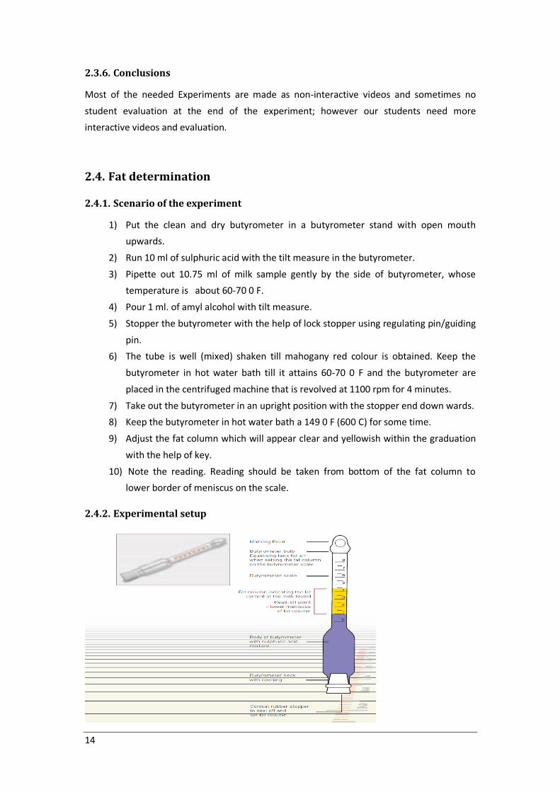
2.4. Fat determination


1) Put the clean and dry butyrometer in a butyrometer stand with open mouth

upwards.

2) Run 10 ml of sulphuric acid with the tilt measure in the butyrometer.

3) Pipette out 10.75 ml of milk sample gently by the side of butyrometer, whose

temperature is about 60-70 0 F.

4) Pour 1 ml. of amyl alcohol with tilt measure.

5) Stopper the butyrometer with the help of lock stopper using regulating pin/guiding

pin.

6) The tube is well (mixed) shaken till mahogany red colour is obtained. Keep the

butyrometer in hot water bath till it attains 60-70 0 F and the butyrometer are

placed in the centrifuged machine that is revolved at 1100 rpm for 4 minutes.

7) Take out the butyrometer in an upright position with the stopper end down wards.

8) Keep the butyrometer in hot water bath a 149 0 F (600 C) for some time.

9) Adjust the fat column which will appear clear and yellowish within the graduation

with the help of key.

10) Note the reading. Reading should be taken from bottom of the fat column to

lower border of meniscus on the scale.


16

2.5. Determination of Total Nitrogen (Kjeldal method)


1) Digestion burner setting. Conduct digestion over heating device that can be

adjusted to bring 250 mL H2O at 250 to rolling boil in ca 5-6 min.

2) Digestion. Digest at least 20 minutes or until white fumes appear in flask. Next,

increase burner setting half way to maximum setting determined in (a) and heat

for 15 minutes. Next, increase heat to maximum setting determined in (a). When

digest clears (clear with light blue-green color), continue to boil 1-1.5 hr at

maximum setting (total time ca 1.8-2.25 hr).

3) Distillation. Turn on condenser water. Add 50 mL H3BO3 solution with indicator

to graduated 500 mL Erlenmeyer titration flask and place flask under condenser tip

so that tip is well below H3BO3 solution surface. To room temperature diluted

digest, carefully add 75 mL 50% NaOH down sidewall of Kjeldahl flask with no

agitation. NaOH forms clear layer under the diluted digest. Immediately connect

flask to distillation bulb on condenser. heat until all NH3 has been distilled (>150

mL distillate; >200 mL total volume). Titrate H3BO3 receiving solution with

standard 0.1000N HCL solution to first trace of pink. Lighted stir plate may aid

visualization of end point. Record mL HCL to at least nearest 0.05 ml.

Nitrogen Recovery Verification

Run nitrogen recoveries to check accuracy of procedure and equipment.

1) Nitrogen loss. Use 0.12 g ammonium sulfate and 0.85 g sucrose per flask. Add all

other reagents as stated in Sample Preparation. Digest and distill under same

conditions as for a milk sample. Recoveries shall be at least 99%.

2) Digestion efficiency. Use 0.16 g lysine hydrochloride or 0.18 g tryptophan, with

0.67 g sucrose per flask. Add all other reagents as stated in Sample Preparation.

Digest and distill under same conditions as for milk sample. Recoveries shall be at

least 98%.

Calculations

Calculate results as follows:

1.4007 x (mL HCL, sample - mL HCL, blank) x normality HCL

Nitrogen, % = --------------------------------------------------------------------

g sample

Multiply percent nitrogen by factor 6.38, to calculate percent "protein." this is "protein" on

a total nitrogen basis.

Maximum recommended difference between duplicates is 0.03% "protein."

17

Repeatability and Reproducibility Values

For method performance parameters obtained in collaborative study of this method Sr =

0.014, SR = 0.017, RSDr = 0.385%, RSDR = 0.504%, r value = 0.038 and R value = 0.049.


18

Chapter 3: Previous experiments in Molecular Biology

3.1. Nucleic acid Extraction


DNA & RNA are extracted from human cells for a variety of reasons. With a pure sample of

DNA you can test a newborn for a genetic disease, analyze forensic evidence, or study a

gene involved in cancer, while RNA samples can be used to test for gene expression of some

genes that might cause cancer or any other disease.


1) Apply extraction buffer to the samples

2) Centrifugation & separation of the supernatant

3) Apply ice cold 100 % Iso-Propanol (for RNA precipitation) or ice cold 100% ethanol

(for DNA precipitation)

4) Centrifugation & separate the pellet

5) Evaporate any alcohol remnant.

6) Dissolve your nucleic acid in sterile water

7) Measure nucleic acid concentration at 260nm & its protein contamination at 280

nm and finally its purity as a ratio between the 2 readings (260/280) it must exceed

1.6 to be suitable for use in PCR & other molecular biology techniques.


DNA Extraction:

http://mwsu-bio101.ning.com/forum/topics/virtual-genetics-labs


19

Hot shot method for DNA extraction

Materials required

Morter and pestle, micropipettes, tips, 1.5 ml vials, 0.5 Mm NaOH, 1M TRIS

HCl, centrifuge.

1) Take 100 µl micropipette

2) Insert a fresh tip

3) Open the bottle of 50 m M NaOH and pipette out 100 µl


5) Open a fresh vial

6) Pour 100 µl in a vial.

7) Close the vial

8) A zebra fish picked from the aquarium

9) Place the fish on the working bench

10) A knife is wiped with cotton

11) A small portion of the fin is cut return back the fish in the aquarium

12) The piece of fin is placed into a morter

13) Fin are crushed with pestle

14) Take a spatula and wipe it with cotton

15) Take the crushed fins with spatula and transfer to the vial of NaOH

16) A needle is taken and pierced the lid of the vial

17) Place the vial in a rack

18) Switch on the water bath and adjust the timer for 20 min and temperature for

950C

19) Put the vial in the water bath

20) After incubation time up, take the vial out of the incubator

21) The vial is placed on the working bench

22) The needle is taken and the vial is kept in an ice tray for 4-5 min

23) Take 10 µl micropipette and insert a fresh tip

24) Open the bottle of tris-HCl

25) Pipette out 10 µl of HCl

20

26) The vial is taken out from the ice box

27) Open the vial and add HCl

28) The centrifuge is opened

29) Put the vial of the sample

30) Equal amount of water is added to a new vial and kept in the centrifuge in order to

balance it

31) Put the vial of water adjacent to the sample vial in the centrifuge inorder to

balance

32) Adjust timer for 10 min and speed at 5000 rpm then press the start button

33) After 10 min up open the centrifuge and take the vial

34) The vial is kept in a rack

35) Take 100 µl micropipette


37) Open the bottle of 50 m M NaOH and pipette out 100 µl

38) Open the sample vial and pipette out the supernatant

39) Keep the vial in the rack

40) Open a new vial and pour 100 µl.

41) Close the vial and put it in the rack


RNA Extraction:

http://amrita.vlab.co.in/?sub=3&brch=186&sim=718&cnt=1382


http://amrita.vlab.co.in/?sub=3&brch=186&sim=718&cnt=1382

21

3.2. PCR , Rt PCR & Real time PCR


PCR (short for Polymerase Chain Reaction) is a relatively simple and inexpensive tool that

you can use to focus in on a segment of DNA and copy it billions of times over. PCR is used

every day to diagnose diseases, identify bacteria and viruses, match criminals to crime

scenes, and in many other ways.


1) DNA (Or RNA Extraction)

2) Apply nucleic acid samples + Master mix (Taq polymerase+ Nucleotides+ buffer+

primers+ water) we need reverse transcriptase with RNA samples

3) Incubate the previous mix in the thermal cycler (conventional PCR or the light

cycler (real time PCR)

4) Analysis (real time PCR)/ gel electrophoresis then analysis (Conventional PCR)




22

PCR

http://www.youtube.com/watch?v=KpWs7QLkAFU

Requirements

Ice box, RNAase free DNAase and water 10xbuffer, plasmid template, forward primer,

reverse primer, dNTPs, taq polymerase, pcr sample, thermal cycler

1) All vials kept in the ice tray.

2) Take micropipette and adjust volume to 37.5 µl


4) Open the vial of RNAase

5) Pipette out RNAase

6) Reclose the vial and place it in the ice tray.

7) Open the vial of pcr sample

8) Add the pipette solution to 0.5 ml pcr sample

9) Close the vial of sample

10) Place it in ice box.

11) Remove the used tip

12) Take micropipette and adjust volume to 5 µl and insert a new tip

13) Open the vial of 10x buffer and pipette out 10x buffer


15) Take micropipette, adjust volume to 1 µl and insert a new tip

16) Open the vial of plasmid and pipette out 1 µ of plasmid


18) Take micropipette and insert a new tip

19) Open the vial of plasmid and pipette out 1 µ of plasmid



22) Open the vial of Dtnp ase and pipette out 2 µl of Dtnp ase



25) Open the vial of forward primer and pipette out 2 µ of forward primer



28) Open the vial of Reverse primer and pipette out 2 µ of Reverse primer



31) Open the vial of Taq polymersase and pipette out 5 µl of Taq polymersase


33) Mix well with pipette

23

34) Open the thermal cycler

35) Put the sample inside

36) Close the thermal cycler

37) Press the start button to start the run.

38) After the run up

The sample is now ready for gel electrophoresis.

3.2.4. Software

Interactive Flash player

http://learn.genetics.utah.edu/content/labs/microarray/

3.2.5. Interfacing

Mouse

3.2.6. Conclusions

Most of the needed Experiments are made as low quality interactive videos; however our

students need higher quality INTERACTIVE videos to be more interesting & Fruitful

3.3. Gel electrophoresis


Separation of the different DNA fragments according to their sizes. Sort and measure DNA

strands by running gel electrophoresis experiment.


1) Prepare the supporting medium (Agarose gel, cellulose acetate or poly acrylamide

gel).

2) Prepare suitable buffer.

3) Apply your samples

4) Apply electric current

5) Analysis



http://learn.genetics.utah.edu/content/labs/gel/



http://learn.genetics.utah.edu/content/labs/gel/

24

3.3.4. Software



3.3.5. Interfacing

Mouse

3.3.6. Conclusions

Most of the needed Experiments are made as non-interactive videos however our students

need higher quality INTERACTIVE videos to be more interesting & Fruitful

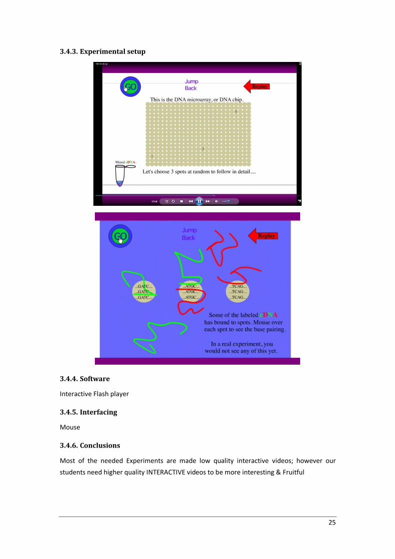
3.4. DNA Microarray

DNA Microarray


DNA microarrays (Chips) are used to investigate everything from cancer to pest control. Use

a DNA microarray to investigate the differences between a healthy cell and a cancer cell.

One common application of DNA chips is to determine which genes are activated and which

genes are repressed.


1) mRNA Extraction

2) Convert mRNA to dye labeled cDNA (different dye for each sample)

3) Apply to DNA microarray (DNA chip) that made of spots, each spot represent a

single stranded DNA of certain gene that can base pair with the labeled cDNA

4) Analysis


25


3.4.4. Software


3.4.5. Interfacing

Mouse

3.4.6. Conclusions

Most of the needed Experiments are made low quality interactive videos; however our

students need higher quality INTERACTIVE videos to be more interesting & Fruitful

26

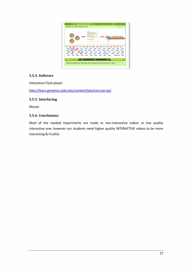
3.5. DNA Finger printing & RFLP


DNA RFLP test s for the DNA variations that can be used to create DNA profile and

individuals ID, while the DNA fingerprinting compare DNA profiles from different individuals


1) DNA EXTRACTION

2) DNA CUTTING + Separation

3) DNA Transfer To Membrane

4) Probe Hybridization

5) ANALYSIS


http://geneed.nlm.nih.gov/topic_subtopic.php?tid=37&sid=38

http://www.yourgenome.org/downloads/animations.shtml

http://geneed.nlm.nih.gov/topic_subtopic.php?tid=37&sid=38

http://www.yourgenome.org/downloads/animations.shtml

27

3.5.4. Software



3.5.5. Interfacing

Mouse

3.5.6. Conclusions

Most of the needed Experiments are made as non-interactive videos or low quality

interactive one; however our students need higher quality INTERACTIVE videos to be more

interesting & Fruitful


28

Chapter 4: Previous experiments in Chromotography

4.1. Quantitavie HPLC analysis of rosmarinic acid in extracts of

Melissa officinalis


Students should be able to understand and imagine how could they detect the

concentration of a major compound (rosmarinic acid) in a herbal extract using sophisticated

equipment as HPLC. They should understand the experimental details as extraction

procedures, sample preparation, serial dilutions, calibration curves, setting up HPLC, and the

interpretation of the results.


1) Tools and chemicals: standard rosmarinic acid, acetonitrile, formaldehyde,

volumetric flask10ml, conical flask 50ml, glass cylinder 50ml, funnel, filter papers,

hot plate, beaker,

2) Introductory page about the equipment and its different parts.

3) Preparation of water extract of fresh Melissa officinalis (the herb of interest).

4) Preparation of a stock solution of rosmarinic acid (0.2 mg/ml).

5) Preparation of serial dilutions from the stock solution (0.1, 0.05, 0.025 mg/ml).

6) Setting up the separation parameters (time, mobile phase, flow rate, wavelength

of detection, range of DAD scanning, column choice and mode of elution).

7) Preparation of a calibration curve from the standard's data.

8) Detection of rosmarinic acid concentration in the extract from the calibration

curve.


Extraction

1) Weigh 2 gm of fresh Melissa officinalis herb.

2) Hold a 50 ml glass cylinder and pour 20 ml of distilled water in it.

3) In a 100 ml glass beaker pour the 20 ml of water.

4) Turn on the hot plate.

5) Put the beaker onto the hot plate until the water starts to boil.

6) Remove the beaker form the hot plate.

7) Put the previously weighed herb in the beaker and wait for 5 minutes.

8) Put a filter paper in a glass funnel and wet it with some water.

9) Set the funnel on a 50 ml conical flask and pour the contents of the beaker in it.

29

10) The filtrate in the flask is the water extract of the herb.

Preparation of the stock solution

11) Hold the box containing standard rosmarinic acid and with a spatula accurately

weigh 2 mg of it.

12) Put the weighed rosmarinic acid in a beaker containing 10 ml of distilled water.

This is the stock solution of the standard acid (0.2 mg/ml).

Preparation of serial dilutions of the standard

13) In 5 ml volumetric flask, pour 2.5 ml of the stock solution and complete the

volume to the mark with distilled water (0.1 mg/ml).

14) Repeat the previous step but with 1.25 ml, 0.625 ml of the stock solution 0.05,

0.025 mg/ml, respectively).

Setting up equipment parameters of the experiment

15) Prepare the mobile phase as follows: solution A (acetonitrile), solution B (water

containing 2.5% acetonitrile and 0.5% formic acid), add 60 ml of solution A to 140

ml of solution B.

16) Turn on the sonicator and put the bottle containing the prepared mobile phase in

it for 15 minutes.

17) Adjust the flow rate of the pump to 1 ml/min.

18) Choose isochractic elution from the panel of the elution modes (isochractic or

gradient).

19) Adjust the wavelength of the UV detector at 254 nm and the DAD at scanning

from 200-550 nm.

20) Setup the run time at 10 minutes.

21) Steps 17-20 are all made on one table (parameters) that appear in one step.

Separation process

22) Hold a reversed phase (RP) analytical column and fix it to the main equipment.

23) Hold the HPLC syringe in your hand and withdraw 10 µl from the 0.1 mg/ml

solution.

24) Insert the syringe into the injection loop and press on its piston.

25) Press on the inject button.

26) The chromatogram starts to appear on the computer screen.

27) Repeat steps 23-25 with the 0.05, 0.025 mg/ml solutions.

28) The computer will give the results for the peak area for each concentration and

the retention time (Rt) for rosmarinic acid (7.04 min)

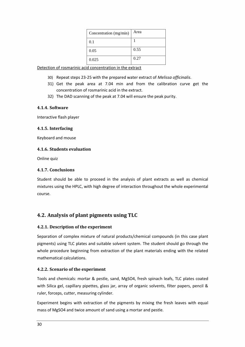
Calibration curve

29) Draw a calibration curve of the peak area (y-axis) and concentration (x-axis) which

must be a straight line passing through the origin. Let the values be as follow:

30

Concentration (mg/min) Area

0.1 1

0.05 0.55

0.025 0.27

Detection of rosmarinic acid concentration in the extract

30) Repeat steps 23-25 with the prepared water extract of Melissa officinalis.

31) Get the peak area at 7.04 min and from the calibration curve get the

concentration of rosmarinic acid in the extract.

32) The DAD scanning of the peak at 7.04 will ensure the peak purity.

4.1.4. Software


4.1.5. Interfacing

Keyboard and mouse


Online quiz

4.1.7. Conclusions

Student should be able to proceed in the analysis of plant extracts as well as chemical

mixtures using the HPLC, with high degree of interaction throughout the whole experimental

course.

4.2. Analysis of plant pigments using TLC


Separation of complex mixture of natural products/chemical compounds (in this case plant

pigments) using TLC plates and suitable solvent system. The student should go through the

whole procedure beginning from extraction of the plant materials ending with the related

mathematical calculations.


Tools and chemicals: mortar & pestle, sand, MgSO4, fresh spinach leafs, TLC plates coated

with Silica gel, capillary pipettes, glass jar, array of organic solvents, filter papers, pencil &

ruler, forceps, cutter, measuring cylinder.

Experiment begins with extraction of the pigments by mixing the fresh leaves with equal

mass of MgSO4 and twice amount of sand using a mortar and pestle.

31

Extraction of the resulting powder with acetone and transfer of the clear acetone

supernatant to a small vial.

Prepare the TLC plate for use, using the cutter, pencil, and a ruler.

Prepare different solvent systems in the glass jars using the cylinder and filter paper.

Start spotting the sample (acetone extract) using capillary pipette on the start line together

with authentic Chlorophyll a, b and xanthopyll.

Place different TLC plates in the different solvent systems and wait until the solvent front

reach the plate end.

Remove the plates and allow to dry, then examine which solvent system separate best &

calculate the Retardation factor (Rf) for each component.


Sample extraction

1) Put 0.5 gm fresh spinach leaves in the mortar, add 0.5 gm MgSO4 and 1 gm sand to

the leaves

2) Hold the pestle in your hand, start to grind and mix the components in the mortar

with the pestle till you reach fine green powder.

3) Bring a one glass test tube and a bottle containing acetone.,

4) Hold a 5 ml pipette in your hand.

5) Put the pipette in the acetone bottle and withdraw 2 ml.

6) Transfer this 2 ml into the empty test tube.

7) With a metal spatula transfer the green powder from the mortar into the test tube

containing the acetone.

8) Hold the tube with your hand.

9) Start vigorous shaking.

10) Put the tube in a rack and allow it to stand for 15 minutes.

11) Hold a glass pipette in your hand.

12) Withdraw the clear green acetone supernatant and transfer it in a small glass vial.

13) Label the vial.

Preparation of TLC plates

14) Hold the TLC pack with your hand and take off several plates.

15) Hold the pencil and the ruler then start drawing the front line on the plates.

16) With the pencil make a mark for the place of each spot (sample and authentic) on

the front line.

Solvent system preparation

17) Start preparing the solvent systems: get three clean 10 ml glass cylinders.

32

18) The first solvent system (60% petroleum ether/16% cyclohexane/10% ethyl

acetate/10% acetone/4% methanol.)

19) The student should calculate the exact amount of each solvent to prepare 10ml.

20) Hold a 10 ml glass pipette and withdraw 6 ml petroleum ether.

21) Transfer them to the cylinder.

22) Hold a 2 ml pipette and withdraw 1.6 ml cyclohexane, 1 ml ethyl acetate, 1 ml

acetone and 0.4 ml methanol. Each time add the withdrawn solvent to the

petroleum ether in the cylinder.

23) Hold the cylinder containing the mixture in your hand and shake well.

24) Get a clean glass jar and open it.

25) Hold the cylinder in your hand.

26) Add the solvent to the cylinder in the jar.

27) Get a small filter paper.

28) Put it in the jar with the solvent.

29) Close the jar thoroughly.

30) Repeat the previous steps with the other solvent mixtures (e.g. hexane:acetone

7:3, cyclohexane:acetone:ether 5:2.5:2.5).

Sample application (spotting)

31) Bring the capillary pipette box and take one.

32) Hold the glass vial containing the acetone extract and gently dip the capillary

pipette in it.

33) On the sample mark on the TLC plate gently press the capillary pipette remove it

and repress again several time until a sufficient spot is produced.

34) Repeat the previous step with each authentic.

35) Make sure that each plate has a sample spot, authentic chlorophyll a spot,

authentic chlorophyll b spot, authentic xanthophyll spot.

36) Gently open each jar.

37) With a forceps take each plate and hold it so that the front line is downwards and

place it in the jar.

38) Repeat the previous step with each solvent mixture you had prepared.

Development of the TLC plate

39) Solvent will rise slowly upward against gravity onto the plate.

40) Throughout the course of solvent rising the sample spot will resolve into different

colors mainly chlorophyll a (first), chlorophyll b (second), xanthophyll (last), and

each authentic should rise and move exactly as its counterpart in the sample

mixture.

41) Different solvent systems will resolve the different pigments in different patterns

and distances.

33

42) When the solvent line reaches the end of the plate, hold the forceps in your hand,

open the jar gently, remove the plate.

43) Put the plate on the bench and allow to dry.

Rf calculation

44) With a ruler measure the distance travelled by each spot from the front line and

measure the distance from the front line to the solvent front and divide the 2

values to get the Rf for each component.

45) Compare the Rf of each component with the authentic in the same plate and with

Rfs with other solvent system.

4.2.4. Software


4.2.5. Interfacing

Keyboard and mouse


Online quiz

4.2.7. Conclusions

Student should be able to proceed in the analysis of plant extracts as well as chemical

mixtures using the simple TLC tool, with high degree of interaction throughout the whole

experimental course

4.3. The Separation and Identification of Some Brominated and

Chlorinated Compounds by GC/MS


The experiment will focus on teaching undergraduate students the operating principles of

Gas Chromatography-Mass Spectrophotometer (GC-MS). The students should be introduced

to the main components of the machine. They should be instructed on how each component

function under normal operating conditions. The experiment should introduce to the

students different applications of GC-MS. Moreover, the outcomes below should be

achieved by applying the experiment.


Laboratory tools

The unknown compounds used in the experiment are listed in the following table.

34

Tetrachloroethylene: The solvent was GC Resolv grade hexane

CAUTION: All procedures with the chemicals—making up solutions, dilutions, etc.—should

be carried out in an efficient fume hood. Students should wear protective lab coats, goggles,

and gloves.

The GC column in this instrument is a DB-5 coated capillary column 30 m long, 0.25 mm i.d.

and 0.25 mm film.

All tools of the lab should be illustrated and when you point the mouse to each requirement

of the experiment its name should appear.


1) A brief introduction to the instrument and the experiment description.

2) Presentation of the equipment with its different parts followed by moving through

each part with magnification and question on each part (interaction).

3) The students are provided with an unknown solution, which contains four or five of

the eight compounds listed in the table.

4) A suitable concentration is obtained by using a dropper to add one or two drops of

each compound (approximately 50–100 µL) to 10 mL of hexane and then diluting

the obtained solution 1:1000 with hexane.

5) The dilution is achieved by adding 1.0 mL of the solution to 1.0 mL of hexane. (The

1.0 mL is measured using a 10-mL syringe).

6) Move to the injection port of the equipment and start injecting (student

interaction). One microliter of the final solution is injected into the GC/MS system.

35

7) To prevent cross-contamination of samples the students are told to rinse the 10-

mL syringe five times with solvent both before and after sample injection).

8) The students obtain a chromatogram that shows the separation of the unknowns

and they print out a mass spectrum for each of the unknown compounds in their

mixture.

9) GC Method

For all of these experiments the following GC program is used: 40 to 70 °C at 10°/min,

70 to 100 °C at 5°/min, and 100 to 180 °C at 10°/min. GC run time was 18 min. The

transfer line temperature between the GC and MS was set at 270 °C. The MS

source temperature was set at 170 °C, and the splitless injection mode was used.

10) MS Method

The instrument was set to operate in the positive ion mode with electron impact as the

ionization method. The mass range was scanned from 50 to 250 Daltons (Da) with

a 3.00-min solvent delay.

11) The students are asked to calculate the expected relative intensities for the peaks

within patterns due to ions containing (i) between one and four chlorine atoms

and (ii) between one and four bromine atoms. Comparison of these relative

intensities with their experimentally obtained data, coupled with the information

that the unknowns contain only either all chlorine atoms or all bromine atoms,

makes identification of the ions in the spectra relatively simple. After the ions are

identified the students are asked to write down the molecular ion and the most

important fragmentation reactions. From this information they can draw

conclusions regarding the identity of the unknowns in most cases. If the GC/MS

equipment has a mass spectral database (library) associated with it they can use

the library for confirmation of their proposed structures. For three of the

unknowns, as explained below, structure identification is not quite so simple

because the unknowns do not show molecular ions in the mass spectra. In these

cases access to a mass spectral database is most helpful and allows simple

identification of the compounds.

4.3.4. Hardware

Desktop or laptop.

4.3.5. Software


4.3.6. Interfacing

Laptop or desktop screen, keyboard and mouse

36


Online quiz

4.3.8. Conclusions

After running the experiment, the student will be familiar with different components of GC-

MS instrument and will get experience in the technique of GC-MS the students could

interpret the mass spectral data to obtain the identity of the unknowns. The interpretation

of the mass spectra (identification of molecular ions and major fragment ions) is simplified

by the presence of the varying numbers of chlorine and bromine atoms, which produce

patterns of peaks in the mass spectra. The relative intensities of the peaks within the

patterns are characteristic of the number of chlorine or bromine atoms.

Chapter 5: Previous experiments in Instruments analysis

5.1. The virtual mass spectrometry laboratory (VMSL)


It is an interactive internet education tool used to teach mass spectrometry. It is a

collaborative project between university of Pittsburgh and Carnegie Mellon University

through a grant by National science foundation.


In VMSL the student can learn about the different VMSL mass spectrometers and sample

preparation using step by step guides consisting of video and other documents.


http://svmsl.chem.cmu.edu/vmsl/maldi/maldi.html

http://svmsl.chem.cmu.edu/vmsl/maldi/maldi.html

37

5.1.4. Interfacing

Students can see pictures of the instrument and watch videos describing different types of

mass spectrometry

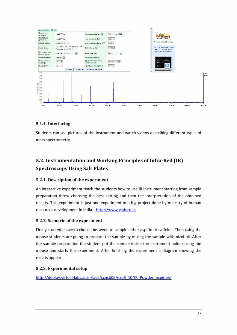
5.2. Instrumentation and Working Principles of Infra-Red (IR)

Spectroscopy Using Salt Plates


An interactive experiment teach the students how to use IR instrument starting from sample

preparation throw choosing the best setting and then the interpretation of the obtained

results. This experiment is just one experiment in a big project done by ministry of human

resources development in India. http://www.vlab.co.in


Firstly students have to choose between to sample either aspirin or caffeine. Then using the

mouse students are going to prepare the sample by mixing the sample with nizol oil. After

the sample preparation the student put the sample inside the instrument holder using the

mouse and starts the experiment. After finishing the experiment a diagram showing the

results appear.


http://deploy.virtual-labs.ac.in/labs/ccnsb06/exp6_10/IR_Powder_exp6.swf

http://www.vlab.co.in/

http://deploy.virtual-labs.ac.in/labs/ccnsb06/exp6_10/IR_Powder_exp6.swf

39

5.2.4. Interfacing

Students use mainly the mouse to choose between sample and to move objects during the

experiment.

5.3. Nuclear magnetic resonance spectroscopy and evaluation of

simple 1H NMR spectra of select organic compounds


HNMR is an instrument used to predict the structure of organic compounds. In a project

created by ministry of human resources development in India an interactive experiment

teach the students how to use the instrument starting from sample preparation throw

choosing the best setting and then the interpretation of the obtained results.

http://www.vlab.co.in


Firstly, the student chooses one sample using the mouse between benzene, acetaldehyde,

or ethyl acetate. After that the sample transfers to the instrument tube by clicking on load

sample button. By clicking on start, the instrument starts bombarding the sample by

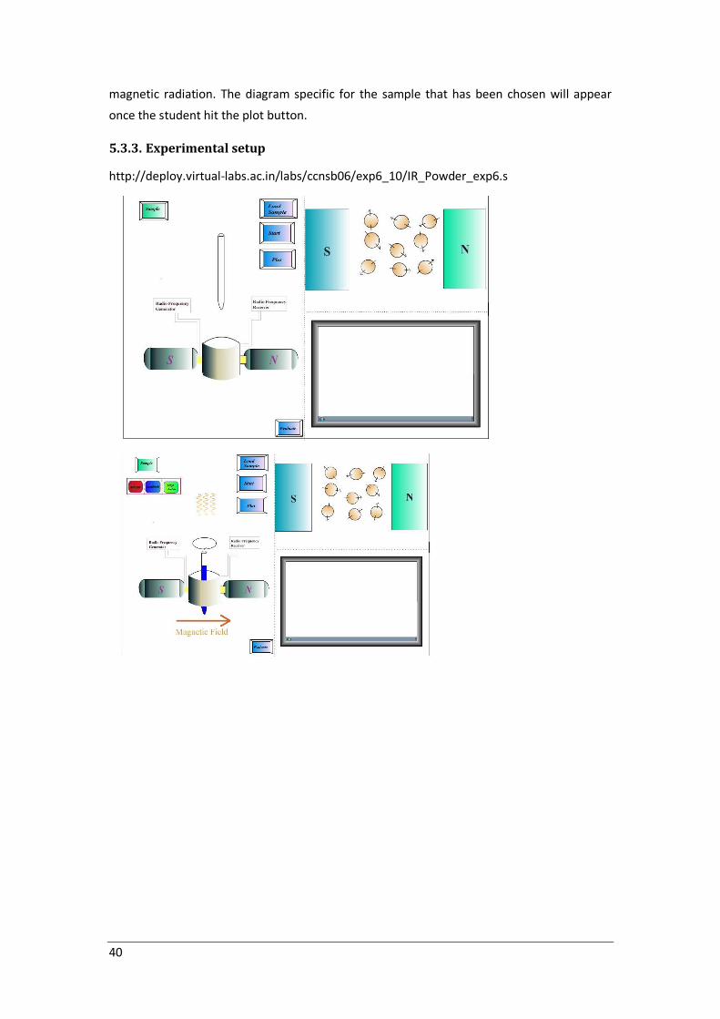
40

magnetic radiation. The diagram specific for the sample that has been chosen will appear

once the student hit the plot button.


http://deploy.virtual-labs.ac.in/labs/ccnsb06/exp6_10/IR_Powder_exp6.s

41

5.3.4. Interfacing

Students use mainly the mouse to choose between sample and to move objects during the

experiment.

42

Chapter 6: Previous experiments in Immunochemistry

6.1. ELISA direct


To detect presence of biomolecules or antigens in samples, Detection of very low

concentrations of antigens to detect certain diseases.


Laboratory tools

Micropipettes rack for micropipettes pipette tip box beaker for wastes incubator absorbent

paper ELISA plate reader microliter well plate

Ice box contains 6 vials of antigen, antibody, substrate, stop solution, blocking buffer and

PBS(phosphate buffered saline)


of the experiment its name appeared

Experiment steps

1) Take micropipette and rotate the upper button to adjust the volume to 50µl

2) Fix a fresh tip on micropipette.

3) Take the antigen vial from the ice box.

4) Open the vial and pipette out 50 µl

5) Open the lid of microliter well plate.

6) Pour 50 µl of antigen into one well of the microplate

7) Pipette out 50 µl again and pour it in another well

8) Repeat the previous step to fill all the wells with the antigen

9) Reclose the antigen vial and put it in the ice box

10) Incubation steps

a) Cover the microplate in a plastic wrap to seal

b) Adjust the incubator at 37 0C and timer for 2 hours

c) Open the incubator steel door then open the glass door.

d) Take the microplate and put it in the incubator.

e) Close the glass door and steel door of the incubator

f) After 2 hours open the incubator and take the microplate

g) Close the incubator

h) Put the microplate on the table

43

i) Uncover the plastic wrapper

11) Flick the coating solution

12) Place microplate on the table

13) Take micropipette remove the used tip

14) Rotate the upper button to adjust the volume to 200µl

15) Fix a fresh tip

16) Washing steps with PBS

a. Open the cap of PBS bottle from the ice box

b) Pour 200 µl of PBS into one well of the microplate

c) Pipette out 200 µl again and pour it in another well

d) Repeat the previous step to fill all the wells with the PBS

e) Reclose the PBS vial

f) Swirl the microplate

g) Take micropipette and remove PBS by sucking it from the first well and pour

PBS in the waste beaker.

h) Repeat the previous step for all the wells

i) Remove the used tip and replace the micropipette on its rack

j) flik the microplate on a paper towel

17) place microplate on the table

18) Take micropipette and Fix a fresh tip on micropipette.

19) Take the blocking buffer vial from the ice box.


21) Pour 200 µl of blocking buffer into one well of the microplate


23) Repeat the previous step to fill all the wells with the blocking buffer

24) Incubate the microplate at room temperature for 2 hours




28) Fix a fresh tip

29) Follow the washing steps with PBS (a to j)



32) rotate the upper button to adjust the volume to 100µl

33) Take the antibody enzyme conjugate vial from the ice box.



36) Pour 100 µl of antibody enzyme conjugate into one well of the microplate


38) Repeat the previous step to fill all the wells with the antibody enzyme conjugate

44

39) Reclose the antibody enzyme conjugate vial and put it in the ice box

40) Cover the microplate in a plastic wrap to seal

41) Incubate the microplate at room temperature for 2 hours.

42) Uncover the plastic wrapper




46) Wash with PBS steps from (a to j)



49) Take the substrate vial from the ice box.



52) Pour 100 µl of substrate into one well of the microplate


54) Repeat the previous step to fill all the wells with the substrate

55) Reclose the substrate vial and put it in the ice box

56) Cover the microplate with a plastic cover



59) Fix a fresh tip

60) Take the stop solution vial from the ice box.



63) Pour 100 µl of stop solution into one well of the microplate


65) Repeat the previous step to fill all the wells with the stop solution


67) Adjust the plate reader at suitable wave length

68) Put the microplate in the plate reader

69) Record the data.

45

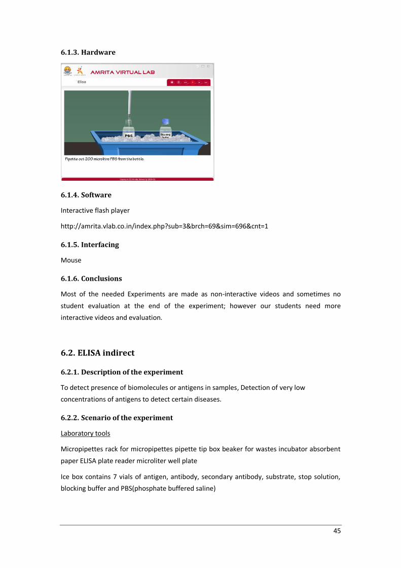
6.1.3. Hardware

6.1.4. Software



6.1.5. Interfacing

Mouse

6.1.6. Conclusions




6.2. ELISA indirect





Laboratory tools



Ice box contains 7 vials of antigen, antibody, secondary antibody, substrate, stop solution,

blocking buffer and PBS(phosphate buffered saline)

46



Experiment steps
























15) Fix a fresh tip

16) Washing steps with PBS

a) Open the cap of PBS bottle from the ice box

b) Pour 200 µl of PBS into one well of the microplate

c) Pipette out 200 µl again and pour it in another well

d) Repeat the previous step to fill all the wells with the PBS

e) Reclose the PBS vial

f) Swirl the microplate

g) Take micropipette and remove PBS by sucking it from the first well and pour

PBS in the waste beaker.

h) Repeat the previous step for all the wells

i) Remove the used tip and replace the micropipette on its rack

j) flik the microplate on a paper towel

47








24) Incubate the microplate at room temperature for 30 min




28) Fix a fresh tip





33) Take the antibody vial from the ice box.



36) Pour 50 µl of antibody into one well of the microplate


38) Repeat the previous step to fill all the wells with the antibody



41) Take the antibody enzyme conjugate vial from the ice box.



44) Pour 100 µl of antibody enzyme conjugate into one well of the microplate


46) Repeat the previous step to fill all the wells with the antibody enzyme conjugate

47) Reclose the antibody enzyme conjugate vial and put it in the ice box










48









65) Fix a fresh tip




69) Take the secondary antibody vial from the ice box.



72) Pour 50 µl of secondary antibody into one well of the microplate


74) Repeat the previous step to fill all the wells with the secondary antibody


76) Cover the microplate with plastic cover

77) Incubate for 2hours at room temperature

78) Follow the washing steps with PBS






84) Pour 75 µl of antibody substrate into one well of the microplate









93) Fix a fresh tip




49








6.2.3. Software



6.2.4. Interfacing

Mouse

6.2.5. Conclusions




6.3. Sandwich ELISA





Laboratory tools


50



Ice box contains 6 vials of, antibody, RBM10-medium, PBMC, PHA, secondary antibody,

alkaline phosphatase labeled antibody, BCIP, blocking buffer and washing buffer

All tools of the lab. Should be illustrated and when you point the mouse to each requirement


Experiment steps



3) Take the cytokine specific antibody vial from the ice box.







10) Incubation steps for 2 hours

a. Cover the microplate in a plastic wrap to seal

b. Adjust the incubator at 37 0C and timer

c. Open the incubator steel door then open the glass door.

d. Take the microplate and put it in the incubator.

e. Close the glass door and steel door of the incubator

f. After time up open the incubator and take the microplate

g. Close the incubator

h. Put the microplate on the table

i. Uncover the plastic wrapper

11) Flick the solution


13) Take micropipette fix new tips


15) Fix a fresh tip

16) Washing steps with washing solution

a) Pipette 200 µl

b) Pour 200 µl of water into the wells of the microplate

c) Pipette out 200 µl again and pour them in another wells

d) Repeat the previous step to fill all the wells with the water

e) Swirl the microplate

51

f) Take micropipette and remove water by sucking it from the first well and

pour water in the waste beaker.

g) Repeat the previous step for all the wells

h) Remove the used tip and replace the multi pipette on its rack

i) flik the microplate on a paper towel

17) repeat washing with washing solution 3 times


19) take the micropipette and adjust 200µl







26) Swirl the plate gently and cover it with a plastic cover


28) Follow incubation steps (i-ix) for 30 min

29) Uncover the plate



32) Take multi pipette remove the used tips

33) Fix a fresh tips

34) Follow the washing steps with water (a to j) 3 times




38) Take the complete RBM10-medium vial from the ice box.



41) Pour 100 µl of RPM10 into one well of the microplate



44) Reclose the RBM-10 vial and put it in the ice box


46) Discard the used tip

47) Fix a fresh tip

48) Take the complete PMC vial from the ice box.



51) Pour 100 µl of PBMC into one well of the microplate

52



54) Reclose the PBMC vial and put it in the ice box

55) Cover the microplate

56) Incubate for 10 min at room temperature


58) Fix a fresh tip

59) Take the complete PHA vial from the ice box.



62) Pour 100 µl of PHA into one well of the microplate



65) Reclose the PHA vial and put it in the ice box

66) Follow the incubation steps for 24 hours with 5 % CO2 incubator (i-ix)





71) Take the cytokine specific secondary antibody vial from the ice box.











82) Fix a new tip

83) Take the alkaline phosphatase labeled Ab vial from the ice box.


85) Pour 50 µl of alkaline phosphatase labeled Ab into one well of the microplate


87) Repeat the previous step to fill all the wells with the alkaline phosphatase labeled

Ab




53



93) Fix a new tip

94) Take the alkaline BCIP vial from the ice box.


96) Pour 50 µl of BCIP into one well of the microplate


98) Repeat the previous step to fill all the wells with the BCIP

99) Incubate the microplate at room temperature for 5 – 30 min



102) Adjust the micropipette at 200 microliter

103) Apply distilled water to all wells of microplate.

104) Put the microplate on the table until the water dry

105) After air drying




6.3.3. Software



6.3.4. Interfacing

Mouse


54

6.3.5. Conclusions




6.4. ELISPOT





Laboratory tools



Ice tray containing vials of antibody, blocking buffer, antigen, substrate, stop solution.


of the experiment its name appeared.

Experiment steps


2) Fix a fresh tip on micropipette

3) Take the antibody vial from the ice box.
















55




13) Take multi pipette fix new tips


15) Fix a fresh tip

Washing steps with water

a) Pipette 200 µl

b) Pour 200 µl of water into the wells of the microplate

c) Pipette out 200 µl again and pour them in another wells

d) Repeat the previous step to fill all the wells with the water

e) Swirl the microplate

f) Take micropipette and remove water by sucking it from the first well and

pour water in the waste beaker.

g) Repeat the previous step for all the wells

h) Remove the used tip and replace the multi pipette on its rack

i) flik the microplate on a paper towel

16) repeat washing with water 2 times


18) take the micropipette and adjust 200µl







25) Swirl the plate gently and cover it with a plastic cover





30) Take multi pipette remove the used tips

31) Fix a fresh tips

32) Follow the washing steps with water (a to j)






56






43) Incubate at room temperature for 2 hours.

44) Remove plastic wrapper.

45) Take the multi pipette and make washing steps with water (a-i)












57) Take multi pipette and make washing steps with water steps (a-i)


59) Take the secondary antibody vial from the ice box.







66) Cover the microplate with plastic cover

67) Incubate for 2hours at room temperature

68) Take multi plate and make washing steps with water steps (a-i)










57


79) Take multi pipette and make washing steps with water steps (a-i)






85) Pour 75 µl of substrate into one well of the microplate








93) Fix a fresh tip and adjust micropipette at 25 microliter











58


6.4.4. Software



6.4.5. Interfacing

Mouse

6.4.6. Conclusions




6.5. Blood grouping


Blood grouping experiment to detect type of the blood group.



Requirements

Alcohol pads

Waste beaker

Lancet



59

Biohazards disposal container.

Anti-A , anti-B and anti-D reagent vials in ice box.

Glass slide

Steps of the experiment

1) Take out the alcohol pad from its packet.

2) Through the waste packet in a waste beaker.

3) Apply the alcohol pad at the site from where blood will be sampled.

4) Put the pad in the waste beaker.

5) Open the lancet cover.

6) Put the waste cover in the waste beaker.

7) Press on the finger of the patient at the same place you sterilized with alc. pad.

8) Prick the fingertip with the lancet.

9) Discard the lancet to the bio hazard disposal container.

10) Squeeze the finger of the patient and put 3 drops of blood on a glass slide.

11) Place the glass slide on the table.

12) Take out the alcohol pad from its packet.

13) Through the waste packet in a waste beaker.

14) Put the pad on the place you pricked it to stop blood flow.

15) Open the cap of the reagent (anti -A) take a drop.

16) Place anti-A drop on the first spot of the blood.

17) Reclose the reagent vial.

18) Open the cap of the reagent (anti -B) take a drop.

19) Place anti-B drop on the second spot of the blood.


21) Open the cap of the reagent (anti -D) take a drop.

22) Place anti-D drop on the third spot of the blood.


24) Take a small glass rod and gently mix the solutions in the first spot.

25) Discard the small glass rod In the biohazard container.

26) Repeat the steps 24 & 25 with the second and third spots.

27) Observe the result within 2 min.

28) Report the type of blood samples.

60


6.5.4. Software



6.5.5. Interfacing

Mouse

6.5.6. Conclusions

This Experiment is made as non-interactive video and has only one question as evaluation at

the end of the experiment but we need more examples for evaluation with interactive

videos.

6.6. Immunohistochemistry (IHC)


Antibody and color staining for certain tissue to detect the cell abnormality for the types of

tumor.


61



Laboratory tools

Tools Chemicals

1 Humidity staining tray

chamber (hstc) 1 TBS wash buffer

2 Plastic pipettes 2 Peroxide block3 %

3 Slides (fixed tissue on them) 3 Primary antibody

4 Covers 4 DAB chromogen

5 Containers for xylene 5 hiDef detection ALk phos

6 Containers for ethanol 6 hiDef detection HRP

7 Slide holder 7 hematoxylin

8 Washing bottle 8 mounting medium

9 Slide holder 9 Xylene

10 Containers (wells) 10 Ethanol 50%, 90%,

100%

11 Microscope

1) Remove the cover of the Humidity staining tray chamber (hstc)

2) Fill it with water and recover it.

3) Fill a tissue well with 200 ml peroxide and submerge the slides in the peroxide

solution for 10 minutes.

4) Fill the washing bottle with TBS wash buffer.

5) Take the slides out of the peroxide solution and rinse it with TBS buffer.

6) Uncover the (hstc) and put the slides in (hstc) and cover the tissues with HiDef

detection amplifier.

7) Recover (hstc) and allow antibody incubation for 10 min.

8) Uncover the (hstc) and take the slides out then recover the (hstc) again.

9) Wash slides with TBS buffer.

10) Uncover the (hstc) and put the slides in (hstc) and cover the tissues with HiDef

detection polymer.

11) Recover (hstc) and allow antibody incubation for min.


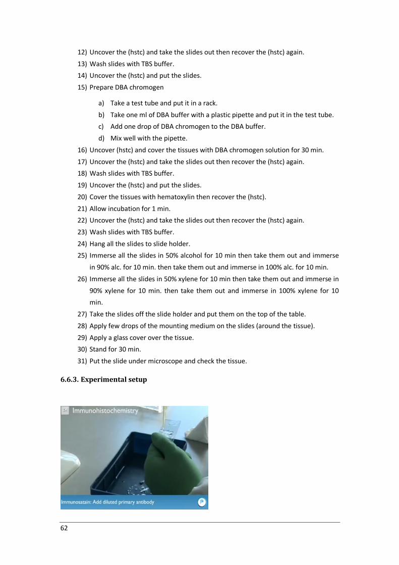
62



14) Uncover the (hstc) and put the slides.

15) Prepare DBA chromogen

a) Take a test tube and put it in a rack.

b) Take one ml of DBA buffer with a plastic pipette and put it in the test tube.

c) Add one drop of DBA chromogen to the DBA buffer.

d) Mix well with the pipette.

16) Uncover (hstc) and cover the tissues with DBA chromogen solution for 30 min.



19) Uncover the (hstc) and put the slides.

20) Cover the tissues with hematoxylin then recover the (hstc).

21) Allow incubation for 1 min.



24) Hang all the slides to slide holder.

25) Immerse all the slides in 50% alcohol for 10 min then take them out and immerse

in 90% alc. for 10 min. then take them out and immerse in 100% alc. for 10 min.

26) Immerse all the slides in 50% xylene for 10 min then take them out and immerse in

90% xylene for 10 min. then take them out and immerse in 100% xylene for 10

min.

27) Take the slides off the slide holder and put them on the top of the table.

28) Apply few drops of the mounting medium on the slides (around the tissue).

29) Apply a glass cover over the tissue.

30) Stand for 30 min.

31) Put the slide under microscope and check the tissue.


63

6.6.4. Software



6.6.5. Interfacing

Mouse

6.6.6. Conclusions




6.7. Double Diffusion Titration


Detect the (titer) concentration of the antigen



Requirements

Weighting balance, Ice box, conical flask, Cotton

Gel bunch, Glass plate beaker measuring cylinder

Tips, micropipettes, Agarose, butter paper


1) A micro pipette is taken and adjust the volume at 20 microliter

2) A fresh tip is inserted

3) label a group of vials as neat 1:2, 1:4, 1:16, 1:32



64

4) Pipette out 20 microliter from the assay buffer

5) Vials labeled as 1:2 is taken from the ice box.

6) Open the vial and add 20 microliter of the assay buffer to the vial

7) Close the vial and return it back to the ice box

8) The bottle labeled as assay buffer is opened.

9) Pipette out 20 microliter from the assay buffer

10) Open the vial and add 20 microliter of the assay buffer to the vial 1:4 repeat that

for all vials.

11) Close the vial and return it back to the ice box

12) The used tip is discarded in the waste beaker

13) Fix fresh tip to the pipette

14) The cap of the vial (antiserum) is opened and pipette out 20 microliter of

antiserum

15) Return the vial of antiserum to the ice box

16) Take the vial (neat)open it and pour 20 microliter of antiserum to it then close it

17) Return it back to the ice box

18) The cap of the vial (antiserum) is opened and pipette out 20 microliter of

antiserum

19) Return it back to the ice box

20) The vial labeled as 1:2 is taken from the ice box open it

21) Add 20 microliter of antiserum to the vial and mix well with the pipette to get the

dilution 1:2

22) 20 microliter of the 1:2 solution is taken by the micropipette.

23) Reclose the vial (1:2) and return it back to the ice box.

24) Take the vial (1:4) from the ice box, open it and add the 20 microliter of the

solution (1:2) has been pipette before.

25) Mix well with the pipette and take 20 microliter from the (1:4) solution , reclose

the vial and return it back to the ice box.

26) The same procedure is repeated for the rest of the vials labeled up to 1:32


28) Preparation of agarose

29) Connect the charge to the electric balance

30) Turn on the electric balance

31) A weighting paper is placed on the weighting balance

32) Press the button of re zero to set the balance at zero weight and neglect the

balance of the paper

33) Open the bottle containing Agarose

34) with a spatula take some of agarose from the bottle and put it on the paper to

weight it

35) add more agarose to reach to the weight 0.1 grams

65

36) The weighted agarose is transferred to a conical flask.

37) The bottle of assay buffer is taken.

38) Pour some of assay buffer in a cylinder to have the volume of 10 ml.

39) The 10 ml of assay buffer is poured into the conical flask containing agarose.

40) The solution is mixed gently

41) The conical flask containing agarose is kept in a microwave oven for 2 min to

solubilize the agarose.

42) A glass plate is placed on a paper and put the plate over it.

43) Take the conical flask and pour 5 ml of the agarose solution on to the gel plate.

44) Let the agarose dry at room temperature for 30 min.

45) Take the template and placed it on a paper.

46) Take the gel bunch with syringe

47) Hold the tip of the gel puncher and place it on the gel corresponding to the

markings on the template

48) Make 7 wells on the gel

49) The wells are marked on opposite side of the plate with a marker

50) The micropipette is taken and adjust to 10 microliter

51) Inset a fresh tip

52) The vial labeled as antigen is taken from the ice box

53) Pipette 10 microliter of antigen solution.

54) Reclose the antigen vial and put it in the ice.

55) Get the plate

56) The well labeled as antigen (Ag) is filled with 10 microliter of antigen solution

taken with the micropipette

57) Discard the used tip and insert another fresh tip.

58) Pipette 10 microliter of neat solution.

59) Reclose the neat vial and put it in the ice.

60) Get the plate

61) The well labeled as neat is filled with 10 microliter of antigen solution taken with

the micropipette


63) Repeat the steps 51 to 56 for all solutions 1:2 to 1:32

64) A petri plate is opened and a small piece of cotton is placed inside it.

65) A small volume of water is squeezed from the wash bottle on to the cotton to

make it wet.

66) The gel plate is taken and is kept inside the chamber.

66


6.7.4. Software


6.7.5. Interfacing

Mouse

6.7.6. Conclusions




6.8. Ouchterlony Double Diffusion


Detect the similarity between antigens



67


Requirements

Weighting balance, Ice box, conical flask, Cotton, Gel bunch

Glass plate beaker measuring cylinder, Tips, micropipettes, Agarose, butter paper,

Incubator, microwave.


1) Take a tissue and put some water on it

2) Take a plate and clean it with the tissue

3) Put the slide on a paper on the table

4) Connect the charge to the electric balance

5) Turn on the electric balance

6) A weighting paper is placed on the weighting balance

7) Press the button of tare to set the balance at zero weight and neglect the balance

of the paper

8) Open the bottle containing Agarose

9) with a spatula take some of agarose from the bottle and put it on the paper to

weight it

10) add more agarose to reach to the weight 0.3 grams

11) The weighted agarose is transferred to a conical flask.

12) The bottle of assay buffer is taken.

13) Pour some of assay buffer in a cylinder to have the volume of 10 ml.

14) The 10 ml of assay buffer is poured into the conical flask containing agarose.

15) The solution is mixed gently

16) The conical flask containing agarose is kept in a microwave oven for 2 min to

solubilize the agarose.

17) A glass plate is placed on a paper and put the plate over it.

18) Take the conical flask and pour 5 ml of the agarose solution on to the gel plate.

19) Let the agarose dry at room temperature for 30 min.

20) Take the template and placed it on a paper.

21) Take the gel bunch with syringe

22) Hold the tip of the gel puncher and place it on the gel corresponding to the

markings on the template

23) Make 3 wells on the gel

24) The wells are marked on opposite side of the plate with a marker Ab, Ag1, Ag2

25) The micropipette is taken and adjust to 10 microliter

26) Inset a fresh tip

27) The vial labeled as antibody is taken from the ice box

28) Pipette 10 microliter of antibody solution.

68

29) Reclose the antigen vial and put it in the ice.

30) Get the plate

31) The well labeled as antigen (Antibody) is filled with 10 microliter of antigen

solution taken with the micropipette


33) Pipette 10 microliter of Ag1 solution.

34) Reclose the neat vial and put it in the ice.

35) Get the plate

36) The well labeled as neat is filled with 10 microliter of Ag1 solution taken with the

micropipette


38) Repeat the steps 51 to 56 for Ag2 solutions.

39) A petri plate is opened and a small piece of cotton is placed inside it.

40) A small volume of water is squeezed from the wash bottle on to the cotton to

make it wet.

41) The gel plate is taken and is kept inside the chamber.

42) Set the incubator temperature at 37 OC and timer for 30 min

43) Put the chamber in incubator

44) Take the plate mention the result after 30 min.


69

6.8.4. Software


6.8.5. Interfacing

Mouse

6.8.6. Conclusions




70

Chapter 7: Previous experiments in Electrochemistry

7.1. Verification of Tafel equation


Tafel equation governs the irreversible behavior of an electrode. It is a relation between the

over potential and the current density:

In this experiment the test electrode is immersed in the solution until equilibrium is reached

and a stable open circuit potential (OCP) is obtained. A DC potential is applied across the

three electrode system making the test electrode negative. Then the potential should be

switched and the corresponding current is recorded using an ammeter connected in series.

The obtained results should be tabulated and graph of the over potential (η) against the Log

value of the current is plotted. From the obtained plot the student should locate the

exchange current Io value which represents the current passed at equilibrium conditions.

Also the student should determine the transfer coefficient for both the anodic and the

cathodic portions.


- The student should read the Theory and the introduction of the experiment.

- The student moves to the pre experimental tab including the procedure and the

material required

- The student moves to the simulator tab

1) Choose an electrode.

2) Choose an over potential.

3) Choose a transfer coefficient.

4) Note the current flow from the Ammeter value.

5) Keeping transfer coefficient constant, find out the Current values by varying over

potential.

6) Find out log values corresponding to each I.

7) Then plot a graph with log I vs η.

8) From the intercept log I0 can be found out. Thus exchange current density I0 can

be calculated for the particular system.

71

9) Exchange current densities for different systems can be calculated.

- The student checks the obtained results to verify the equation according to

the existed tables.


PC provided with internet connection

7.1.4. Software

Internet based simulation (Java)

7.1.5. Interfacing

Mouse and keyboard


The student is evaluated twice first of them is a self evaluation quiz in order to allow the

student to test his understanding to the experiment theory and concept which is not scored.

The second is an assignment for evaluation of the student after the experiment with scoring.

7.1.7. Conclusions

By the end of this virtual lab the student should know:

1) Study about the irreversible behavior of an electrode.

2) Understand the mechanism of electron transfer to an electrode.

3) Determine the current density.

4) Verifying Tafel plot.

Cyclic Voltammetry concepts and application


The goal of this experiment is to get familiar with:

1) Using a modern electrochemical potentiostat to observe the reduction- oxidation

of iron (III) to iron (II) and vice versa under the given potential range.

2) To measure the diffusion coefficient for iron (III).

3) Voltammetric study of neurotransmitter Dopamine via screen printed carbon

electrode

The Cyclic voltammetry is the most widely used technique for acquiring qualitative

information about electrochemical reactions. The power of cyclic voltammetry results from

its ability to rapidly provide considerable information on the thermodynamics of redox

72

processes and the kinetics of heterogeneous electron-transfer reactions and on the coupled

chemical reactions or adsorption processes. The Cyclic voltammetry is often the first

experiment performed in an electroanalytical study. In particular, it offers a rapid location of

redox potentials of the electroactive species and convenient evaluation of the effect of the

media upon the redox process.

In typical cyclic voltammetry, a solution component is electrolyzed (oxidized or reduced) by

placing the solution in contact with an electrode surface and then making that surface

sufficiently positive or negative in voltage to force electron transfer. In simple cases, the

surface is started at a particular voltage with respect to a reference half-cell such as calomel

or Ag/AgCl, the electrode voltage is changed to a higher or lower voltage at a linear rate and

finally, the voltage is changed back to the original value at the same linear rate. When the

surface becomes sufficiently negative or positive, a solution species may gain electrons from

the surface or transfer electrons to the surface. This results in a measurable current in the

electrode circuitry. The result of cyclic voltammetry obtained in form of cycle between

current and potential, potential on X axis and voltage on Y axis.

The obtained peak current can be simply correlated to the diffusion coefficient and

concentration through the following equation

Ip = (2.687 x 105) n3/2 v1/2 D1/2 A C


1) The student starts the experiment with the basic introduction of the cyclic

voltammetry technique and its theory

2) Then the student moves to the setup tab to check the requirements of the

experiment and its experimental setup

3) Then the student moves to the sample tab to check the sample preparation

4) The student moves to the procedure to check the experiment procedure

5) Then to the animation tab to start the animation of the device and the obtained

results

6) The student moves to the perform tab to figure the steps to deal with the

software

7) The student moves to the data analysis tab to analyze the obtained results


PC provided with internet connection

7.1.11. Software

1) Internet based simulation (java & flash)

2) Require analysis software and access to server

73

7.1.12. Interfacing

Mouse and keyboard


Quiz at the end of the experiment

7.1.14. Conclusions

By the end of this experiment the student should know:

1) The basics of the cyclic voltammetry

2) The concept of reversible electrochemical redox behavior

3) The application of the cyclic voltammetry in electroanalytical measurements

74

Chapter 8: Previous experiments in Qualitative Analysis

8.1. Qualitative analysis of anions


This applet is simulates the laboratory experiment to identify samples of unknown anions.

You can also record notification and show the equation of the reactions


1) Using lab bench (select unknown- select reagent)

2) Add comments of notification

3) Show the equation of the reaction

4) General help


http://www.dartmouth.edu/~chemlab/info/resources/qual/soluble.SolubleAppletA.html

http://www.dartmouth.edu/~chemlab/info/resources/qual/soluble.SolubleAppletA.html

75

8.1.4. Software

You need to be using a Java-enabled browser to view this applet.

8.1.5. Interfacing

Mouse and Keyboard

8.2. Qualitative analysis of cations


This applet is simulates the laboratory experiment to identify samples of unknown metal

cations with the same user interface as the anion applet, you can also record notification

and show the equation of the reactions


1) Using lab bench (select unknown- select reagent)

2) Add comments of notification

3) Show the equation of the reaction

4) General help


http://www.dartmouth.edu/~chemlab/info/resources/qual/soluble.SolubleAppletC.html

http://www.dartmouth.edu/~chemlab/info/resources/qual/soluble.SolubleAppletC.html

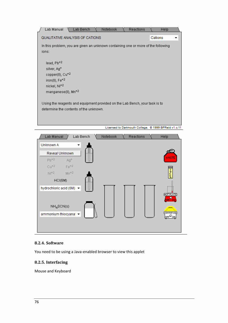
76

8.2.4. Software

You need to be using a Java-enabled browser to view this applet

8.2.5. Interfacing

Mouse and Keyboard

77

Chapter 9: Previous experiments in Material Science

9.1. The virtual XRD laboratory


It is an interactive online learning tool used to teach XRD technique.

Through self-instruction, this module will introduce to student

1) The basics of X-Ray diffraction and the forming of powder patterns.

2) The instrumentation used to perform X-Ray diffraction.

3) How to prepare samples for XRD.

4) How to conduct powder XRD experiments.

5) How to interpret powder X-Ray diffractograms.

In addition, student will have access to a virtual diffractometer which will enable him to try

some simple experiments and visualize their results. The module will assist student to

conduct X-Ray diffraction experiments and interpret their results.


In practice of XRD the student can learn about

1) Sample preparation

2) Safety in X-Ray diffraction

3) Analysis of data

4) Step-by-step operating procedures

5) Virtual XRD


http://www.ammrf.org.au/myscope/xrd/practice/virtualxrd/entryslits.php

Sample preparation

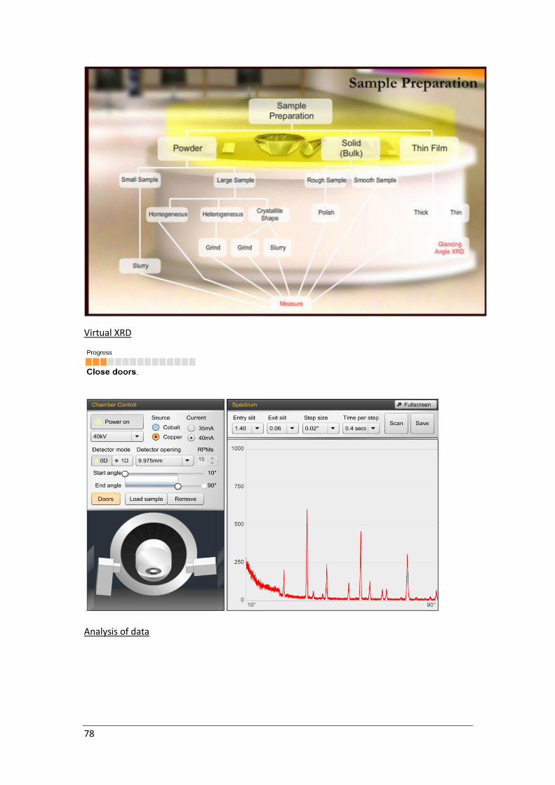
http://www.ammrf.org.au/myscope/xrd/practice/virtualxrd/entryslits.php

78

Virtual XRD

Analysis of data

79

9.1.4. Software

Flash player

9.1.5. Interfacing

Keyboard and mouse


Online MCQ

9.1.7. Conclusions

Student should be able to prepare the sample, carry the experimental using virtual lab and

analysis the data for different samples.

9.2. Instrumentation and Working Principles of SEM


Online learning module for scanning electron microscopy. Through self-instruction, this unit

will introduce student to:

1) The basic principles of SEM operation.

2) The origin of images and their formation.

3) Procedures for collecting and interpreting images.

4) routines for preparing samples for investigation and ways to work safely in an

electronmicroscope laboratory.

Student will also get the opportunity to “play” with a virtual Scanning Electron Microscope

by following the guided instructions. This module will not make student an overnight expert

80

in SEM, but it will provide the essential skills needed to begin experimentation and provide

the scaffolding necessary to become a full-fledged electron microscopist through practice

and perseverance.

At the end of the module menu is an online multiple choice test. student can do this at any

time to determine how much he know about SEM, and repeat it as many times as student

like. The result can be saved and sent to his teacher or supervisor if necessary.


Scanning electron microscopy in practice the student will learn and make the following

1) Principles of SEM operation


3) Virtual SEM

4) Health and safety


http://www.ammrf.org.au/myscope/sem/practice/

http://www.ammrf.org.au/myscope/sem/practice/

82

Interactive simulation of a scanning electron microscope (SEM) imaging welding slag. Shows

the effect of such settings as accelerating voltage, spot size, Z-depth, filament current,

magnification, and astigmatism.

9.2.4. Software

Flash player

9.2.5. Interfacing

Students use mainly the mouse and keyboard


Online multiple choice test

83

9.2.7. Conclusions


analysis the data for different samples

9.3. Instrumentation and Working Principles of TEM


Online learning module for transmission electron microscopy. Through self-instruction, this

unit will help student learn:

1) the basic principles of TEM operation;

2) the origin of images and their formation;

3) to understand electron diffraction and its applications;

4) to understand procedures for collecting and interpreting images;

5) to develop routines for preparing samples for investigation; and

6) how to work safely in an electron microscope laboratory.

Student will also get the opportunity to “play” with a virtual transmission electron

microscope by following the guided instructions. This module will not make student an

expert overnight, but it will provide the background needed to begin experimentation and

provide the scaffolding necessary to eventually become a fully-fledged electron microscopist

through practice and perseverance.

At the end of the module menu is an online multiple choice test. Student can do this at any

time to determine how much you know about TEM, and repeat it as many times as you like.

The result can be saved and sent to your teacher or supervisor.


Transmission electron microscopy in practice the student will learn and make the following

1) Principles of TEM operation


3) Virtual TEM

4) Health and safety


http://www.ammrf.org.au/myscope/tem/practice/virtualtem/

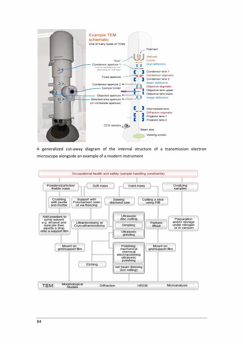
84

A generalized cut-away diagram of the internal structure of a transmission electron

microscope alongside an example of a modern instrument

85

9.3.4. Software

Flash player

9.3.5. Interfacing

Mouse and keyboard


Online multiple choice test

9.3.7. Conclusions


analysis the data for different samples

86

Chapter 10: Previous experiments in Physical Properties

10.1. Boyle's Law and Charles' Law


Investigate the properties of an ideal gas by performing experiments in which the

temperature is held constant (Boyle's Law), and others in which the pressure remains fixed

(Charles' Law). The pressure is controlled through the placement of masses on the lid of the

container, and temperature is controlled with an adjustable heat source.


1) Two modes of the simulation are available; selecting the temperature with

constant weights (pressure) for simulating Charles’ Law; or selecting the masses at

constant temperature for simulating Boyle’s Law. Both choices are available in the

main window.

2) Experimental Then recording the data in the following table:

87

3) Drawing two kinds of plots; Bar Chart and graphs

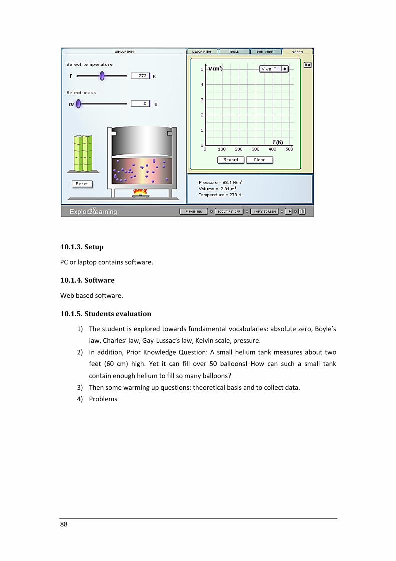
88

10.1.3. Setup

PC or laptop contains software.

10.1.4. Software

Web based software.


1) The student is explored towards fundamental vocabularies: absolute zero, Boyle’s

law, Charles’ law, Gay-Lussac’s law, Kelvin scale, pressure.

2) In addition, Prior Knowledge Question: A small helium tank measures about two

feet (60 cm) high. Yet it can fill over 50 balloons! How can such a small tank

contain enough helium to fill so many balloons?

3) Then some warming up questions: theoretical basis and to collect data.

4) Problems

90

10.2. Gas properties


URL: http://phet.colorado.edu/en/simulation/gas-properties

Via: PhET interactive simulation by university of Colorado Boulder and supported by Royal

Society of chemistry.

1) Predict how changing a variable among P, V, T, and number influences other gas

properties.

2) Predict how changing temperature will affect the speed of molecules.

3) Rank the speed of molecules in thermal equilibrium based on the relative masses

of molecules.


Pump gas molecules to a box and see what happens as you change the volume, add or

remove heat, change gravity, thermodynamics and more. Measure the temperature and

pressure, and discover how the properties of the gas vary in relation to each other.

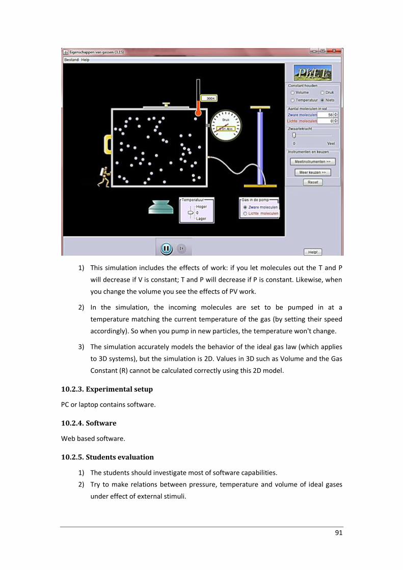
91

1) This simulation includes the effects of work: if you let molecules out the T and P

will decrease if V is constant; T and P will decrease if P is constant. Likewise, when

you change the volume you see the effects of PV work.

2) In the simulation, the incoming molecules are set to be pumped in at a

temperature matching the current temperature of the gas (by setting their speed

accordingly). So when you pump in new particles, the temperature won't change.

3) The simulation accurately models the behavior of the ideal gas law (which applies

to 3D systems), but the simulation is 2D. Values in 3D such as Volume and the Gas

Constant (R) cannot be calculated correctly using this 2D model.



10.2.4. Software

Web based software.


1) The students should investigate most of software capabilities.

2) Try to make relations between pressure, temperature and volume of ideal gases

under effect of external stimuli.

92

3) How to implement the data of this simulation to understand the different basic gas

laws; Boyle’s Law, Gay-Lussac’s Law, Charles’ Law, Graham’s Law of Effusion,

Application of 1st law of thermodynamics, Dalton’s law of partial pressures.

10.3. Balloons & Buoyancy


URL: http://phet.colorado.edu/en/simulation/balloons-and-buoyancy



1) Determine what causes the balloon, rigid sphere, and helium balloon to rise up or

fall down in the box.

2) Predict how changing a variable among P, V, T, and number influences the motion

of the balloons


Experiment with a helium balloon, a hot air balloon, or a rigid sphere filled with different

gases. Discover what makes some balloons float and others sink.

93

1) The rigid sphere and helium balloon have small mass; the hot air balloon has more.

2) The elasticity of the balloon is optimized based on our interviews to be small, but

appropriate. The sim is not designed for calculating elasticity constant.

3) This simulation includes the effects of work: if you let molecules out the T and P

will decrease if V is constant; T and P will decrease if P is constant. Likewise, when

you change the volume you see the effects of PV work.

4) To demonstrate the relationship between n and P (how does P change when I

increase n and keep everything else constant), set the volume constant and add

molecules.

5) To demonstrate the relationship between P vs T, use the heater and keep volume

constant and n constant (by not adding molecules).



10.3.4. Software

Web based software.

94


1) The students should investigate and interpret the relationship between gas law

and buoyancy.

2) How to implement the data of this simulation to understand different phenomena;

Hot air balloons and how do gases in different containers behave in gases fluids?

10.4. The Greenhouse Effect


URL:http://phet.colorado.edu/en/simulation/greenhouse



How do greenhouse gases affect the climate? Explore the atmosphere during the ice age and

today. What happens when you add clouds? Change the greenhouse gas concentration and

see how the temperature changes. Then compare to the effect of glass panes. Zoom in and

see how light interacts with molecules. Do all atmospheric gases contribute to the

greenhouse effect?


1) The sim is based on a simplified model illustrating the core concept behind

greenhouse warming. It shows only 2 types of photons – sunlight photons which

include the visible range of electromagnetic waves and infrared (IR) photons. It

does not model wavelength specific absorption and emission. The model does not

explicitly include specific greenhouse gases.

2) The temperature is measured close to the earth’s surface. The model is calibrated

to match average surface temperatures from the given time periods.

3) The Photon Absorption tab shows simplified processes.

95



10.4.4. Software

Web based software.

96


At the end, the student should be able to:

1) Describe the effect of greenhouse gases on photons and temperature

2) Describe the effect of clouds on photons and temperature

3) Compare the effect of greenhouse gases to the effect of glass panes

4) Describe the interaction of photons with atmospheric gases

5) Explain why greenhouse gases affect temperature

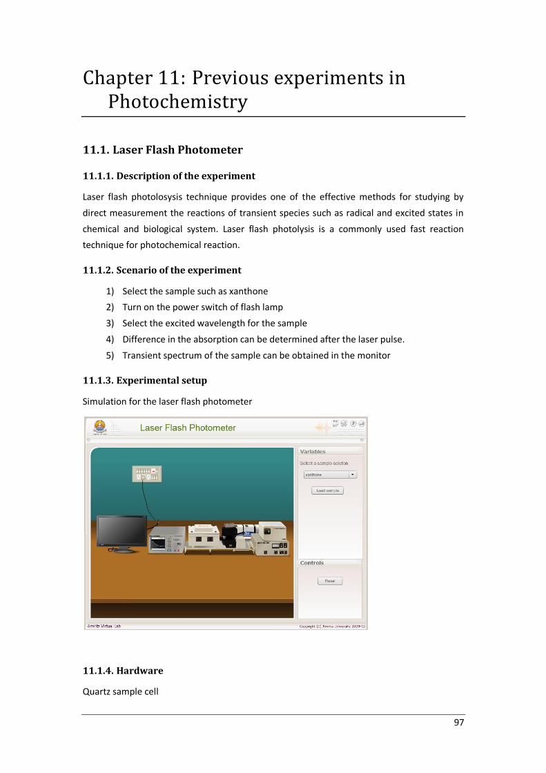
97

Chapter 11: Previous experiments in Photochemistry

11.1. Laser Flash Photometer


Laser flash photolosysis technique provides one of the effective methods for studying by

direct measurement the reactions of transient species such as radical and excited states in

chemical and biological system. Laser flash photolysis is a commonly used fast reaction

technique for photochemical reaction.


1) Select the sample such as xanthone

2) Turn on the power switch of flash lamp

3) Select the excited wavelength for the sample

4) Difference in the absorption can be determined after the laser pulse.

5) Transient spectrum of the sample can be obtained in the monitor


Simulation for the laser flash photometer

11.1.4. Hardware

Quartz sample cell

98

11.1.5. Software

Simulation for software of flash photometer



11.1.6. Interfacing

Mouse


Using multiple choice questions


11.2. Solar Radiation Measurements


The overall goal of the Site Assessment for Solar Energy Utilization Experiment is to learn

how to analyze solar data to assess the suitability of a site for installing a solar energy

system. Moreover, the experiment background and Theory of solar radiation were reported.


1) Go to the “Simulator” link in this experiment.

2) Click the “Start Streaming Live Data” button

3) Watch how the solar data changes over time. It is recommended that the user

watch the data for some time, in order to see changes in the irradiation.

4) “Stop” the experiment.

5) "Export" the data as a Comma Separated Value file (.csv) to Microsoft Excel /

LibreOffice / OpenSpreadsheet or a similar program, or a similar spreadsheet

program.

6) If it is nighttime when you are performing the experiment, or you want to analyze

a longer duration data set, Historical Data is available for download by clicking the

Historical Data button.

7) After importing the data into the spreadsheet

8) Create a graph of the GHI vs. time, DIF vs. time, and DNI vs. time.

9) Find the peak, minimum, and average Irradiance over the data file duration,

10) Calculate the Energy received by the sensor over the duration of the data file.

11) Create a new column titled “Energy”, to the right of the column titled “Irradiance”.

This should be column “C”.



99

12) Find the “Delta t”, or the interval between successive data elements. For our

experiment, this is set to one second.

13) In the second row of the new column, multiply the adjacent Irradiance value by one

second. The formula should look something like “=B2*1”. You can copy and paste this

cell into the other row elements of column “C”, down to the last row of data. Each of

these energy elements approximates the solar energy received over the one second

sampling interval.

14) Find the Total Energy Received over the duration of the time by adding up all of the

energy intervals. This can be done by using a “Sum” formula. This formula will give you

the total energy received over the file duration, in units of Watt-seconds or Joules.

15) Convert the Total Energy Received from Watt-seconds to Watt-hours by dividing the

previous answer by 3600.

16) Check your answers against the values given on the experiment webpage. If they

match, Congratulations!, you have just done your first solar energy site assessment. If

not, go back and check your calculations until the correct answers are obtained. Of

course, for an actual site assessment, data should be collected for a much more

extended duration of time.


This remote trigger experiment collects data from a pyrheliometer and two actual

pyranometers installed at Amrita University, Amritapui Campus. The geographical

coordinates are:

Longitude =76.492016; //units are degrees & Latitude = 9.094258; // units are degrees

100

11.2.4. Hardware

1) Pyranometer - Huskeflux LP02-30 – receptive in the solar spectral band between

285 and 3000 nm.

2) Pyrheliometer - Hukseflux DR01 - receptive in the solar spectral band between

200 and 4000 nm.

3) Custom made dual axis soun tracking mechanism.

4) Data Acquisition Module - Labjack UE9-Pro over Ethernet

11.2.5. Software

Microsoft excel, Libreoffice, openSpread sheet


11.2.6. Interfacing

Mouse


Some examples of assignment

1) Find and analyze local solar data:

2) Find the average hourly Direct Normal Irradiation (DNI), and the

3) Find the average daily DNI.

4) Plot the hourly Direct Normal Irradiation (DNI) using the Graph functions.

101

Chapter 12: Conclusions and recommendations

12.1. Conclusion

In this report the partners in this project did a deep web-based search to survey previous

efforts that have been done to establish web-based electronic chemistry laboratories for

students. In general, I was clear from that web survey that most of what has been found was

made as non-interactive videos and sometimes no student evaluation at the end of the

experiment. Although some interactive work has been found, this work was just for one

separate experiment for each project. The main idea in our project is to create interactive

online experiments not just one. The idea is to gather different experiments from different

chemistry branches and also suitable to different level of students. In fact, we were not able

to find many done example similar to what was in our mind except few projects which did

something similar to what we want to do, For example Virtual Labs at Amrita Vishwa

Vidyapeetham University.

As it is clear from the report, many experiments have been mentioned from Virtual Labs at

Amrita Vishwa Vidyapeetham University as examples of previous experiments done before.

Some other projects were concentrated just on one experiment as the virtual mass

spectrometry laboratory (http://svmsl.chem.cmu.edu/vmsl/maldi/maldi.html) which only

for mass spectroscopy. Other projects concentrated on a branch of chemistry, for example

the Genetic Science Learning Center at The University of Utah which meanly shows a

biochemistry experiments.

In conclusion, although this project won't be the only chemistry e-lab in the world but at

least it will be one among few examples which have a wide collection of chemistry

experiments.

12.2. Technology

12.2.1. Overview

After reviewing the teachers’ requirements, we decided to use Java programming language

to develop the experiments as it satisfies our development requirements like:

1) Powerful language: it will help us create, develop and innovate complicated

scenarios and experiments.

2) Open Source: it doesn’t need any costs for using it on development or deploying.

3) Web based applets: it develops web based applets that can be accessed easily by

the students using web browsers.

102

4) Rich interfaces: it is capable of developing rich, modern and eye-catching graphical

user interfaces and animations.

5) Source code encryption: it encrypts the source code for protection and copyrights.

6) Large community: There is a very large developer community that ensures support

and sustainability.

7) Lots of open source libraries: getting benefits from other experiences.

8) Pre-experience: we already developed similar e-Lab project for physics and

engineering education.

12.2.2. JavaFX

JavaFX provides a powerful Java-based UI platform capable of handling large-scale data-

driven applications. JavaFX applications are completely developed in Java, one of the most

widely deployed technologies with one of the largest developer communities in the world,

while leveraging the power of standards-based programming practices and design patterns.

JavaFX provides a rich set of UI controls, graphics and media API with high-performance

hardware-accelerated graphics and media engines to simplify development of immersive

visual applications.

12.2.3. Adobe EDGE Animate

The eLab Chemistry experiments contain a lot of animations that demonstrate steps and

behaviors, so we used Adobe EDGE Animate to easily create HTML5 animations and

integrate it with Java web view component inside the experiments.

12.2.4. Learning Management System

The eLab Chemistry experiments should be hosted in a place where students/teachers can

access it, also those experiments must be a part of a parent system which enables the

responsible persons to control students access, track their activities and supply the needed

theoretical background and help material to the students, The students also should be able

to do assignments and handle experiments’ reports through this system. For these purposes

it is needed to host these experiments through Learning Management System (LMS).

12.2.5. Moodle Learning Management

The selected Learning Management System is Moodle due to the following:

1) Well Organized

- Dividing content into categories, subcategories and courses.

- Courses contain different content, activities and resources.

- Students can access only courses which they are enrolled in.

- Courses contain different privileges for students, teachers and managers.

- Automatic exams, assignments and grading.

2) Flexible

- Customizable for individual needs as it is open source.

- A lot of modules available.

103

- Easy to integrate modules.

- Disable and enable modules according to needs.

- Easy to customize modules from application to source code level.

- Easy to develop and add modules on development levels.

- Multi-language support

3) Scalable to Any Size

From a few students to millions of users, Moodle can be scaled to support the

needs of both small classes and large organizations. Because of its flexibility and

scalability, Moodle has been adapted for use across education, business, non-

profit, government, and community contexts.

4) Secure

- Different levels of security can be applied.

- Secure core, latest version has no vulnerabilities.

- Secure registration system based on email confirmation or manual

accounts.

- Support for secure SSL system.

- Secure operations and activities among different site privileges and

permissions.

5) Cross Platform Accessibility

- Access from anywhere as a web application.

- Easy accessed from normal PC’s and support for well-known web browsers.

- Support android devices for different screen sizes and devices’ types.

- Support for iOS devices.

6) Open Source & Up-to-Date

- Moodle has php web core which is open source for easy customization.

- Moodle community is very active.

- Continuous modules development.

- Continuous version updates (2 new releases per year).

- Moodle is continually being reviewed and improved on to suit the current

and evolving needs of its users.

7) Documentation

- Rich documentation.

- More detailed content.

- Screenshots support.

- Step by step tutorials.

- Special developer’s documentation.

- Easy online access to source code for customization and development

8) Wide Spread

There are 55245 currently active sites that have registered from 230 countries, 137

Sites are registered in Egypt.

104

9) Versions Usage

10) 2014 best LMS in Top 100 Tools for Learning

- Moodle is voted as best LMS in 2014 and the 12th best learning tool in 2014

top 100 tools.

- Announcement on Moodle website

https://moodle.org/news/

- Top 100 Tools for Learning 2014

http://c4lpt.co.uk/top100tools/

- Moodle is the best of breed

http://c4lpt.co.uk/top100tools/best-of-breed/

12.2.6. Network and Hardware

The selected way to host Moodle Learning Management System is using high availability

clustering to support larger number of concurrent users and maintain high availability. This

cluster is controlled via a head node (cluster server) and database system. The network

traffic to the cluster is controlled using load balancing system, see the following figure.







e-laboratories for chemistry education survey report · e-laboratories for chemistry education...

Documents