e cient adaptive algorithms for an electromagnetic coe ... · e cient adaptive algorithms for an...

Thesis for the Degree of Doctor of Philosophy

Efficient Adaptive Algorithms for anElectromagnetic Coefficient Inverse

Problem

John Bondestam Malmberg

Division of MathematicsDepartment of Mathematical Sciences

Chalmers University of Technologyand University of Gothenburg

Goteborg, Sweden, 2017

Efficient Adaptive Algorithms for an Electromagnetic Coefficient

Inverse Problem

John Bondestam MalmbergISBN 978-91-629-0203-2 (electronic version)ISBN 978-91-629-0204-9 (printed version)

c© John Bondestam Malmberg, 2017.

Department of Mathematical SciencesChalmers University of Technologyand University of GothenburgSE–412 96 GothenburgSwedenTelephone: +46 (0)31-772 10 00

Typeset with LATEX.Printed in Gothenburg, Sweden, 2017 by Ineko AB.

Abstract

This thesis comprises five scientific papers, all of which are focus-ing on the inverse problem of reconstructing a dielectric permittivitywhich may vary in space inside a given domain. The data for the re-construction consist of time-domain observations of the electric field,resulting from a single incident wave, on a part of the boundary of thedomain under consideration. The medium is assumed to be isotropic,non-magnetic, and non-conductive. We model the permittivity as acontinuous function, and identify distinct objects by means of iso-surfaces at threshold values of the permittivity.

Our reconstruction method is centred around the minimization ofa Tikhonov functional, well known from the theory of ill-posed prob-lems, where the minimization is performed in a Lagrangian frameworkinspired by optimal control theory for partial differential equations.Initial approximations for the regularization and minimization are ob-tained either by a so-called approximately globally convergent method,or by a (simpler but less rigorous) homogeneous background guess.

The functions involved in the minimization are approximated withfinite elements, or with a domain decomposition method with finiteelements and finite differences. The computational meshes are refinedadaptively with regard to the accuracy of the reconstructed permittiv-ity, by means of an a posteriori error estimate derived in detail in thefourth paper.

The method is tested with success on simulated as well as labora-tory measured data.

Keywords: coefficient inverse problem, inverse scattering, Maxwell’sequations, approximate global convergence, finite element method,adaptivity, a posteriori error analysis

i

List of included papers

The following papers are included in this thesis:

• Paper I. Larisa Beilina, Nguyen Trung Thanh,Michael V. Klibanov and John Bondestam Malmberg.Reconstruction of shapes and refractive indices frombackscattering experimental data using the adaptivity. Inverseproblems 30:105007, 2014.

• Paper II. Larisa Beilina, Nguyen Trung Thanh,Michael V. Klibanov and John Bondestam Malmberg.Globally convergent and adaptive finite element methods inimaging of buried objects from experimental backscattering radarmeasurements. Journal of Computational and AppliedMathematics 289:371–391, 2015.

• Paper III. John Bondestam Malmberg. A posteriori errorestimate in the Lagrangian setting for an inverse problem based ona new formulation of Maxwell’s system, volume 120 of SpringerProceedings in Mathematics and Statistics, pages 42–53, Springer,2015.

• Paper IV. John Bondestam Malmberg, and Larisa Beilina.An Adaptive Finite Element Method in QuantitativeReconstruction of Small Inclusions from Limited Observations.Manuscript submitted to Applied Mathematics & InformationSciences.

• Paper V. John Bondestam Malmberg, and Larisa Beilina.Iterative Regularization and Adaptivity for an ElectromagneticCoefficient Inverse Problem. Manuscript to appear in theProceedings of the 14th International Conference of NumericalAnalysis and Applied Mathematics.

iii

iv LIST OF INCLUDED PAPERS

The following papers are, for reasons of extent and consistency, notincluded in this thesis:

• John Bondestam Malmberg and Larisa Beilina. Approximateglobally convergent algorithm with applications in electricalprospecting, volume 52 of Springer Proceedings in Mathematicsand Statistics, pages 29–41, Springer, 2013.

• John Bondestam Malmberg. A posteriori error estimation in afinite element method for reconstruction of dielectric permittivity.Preprint.

• Larisa Beilina, Nguyen Trung Thanh, Michael V. Klibanov andJohn Bondestam Malmberg. Methods of QuantitativeReconstruction of Shapes and Refractive Indices fromExperimental data, volume 120 of Springer Proceedings inMathematics and Statistics, pages 13–41, Springer, 2015.

• John Bondestam Malmberg, and Larisa Beilina. Reconstruction ofa Dielectric Permittivity Function Using an Adaptive FiniteElement Method. Proceedings of ICEAA 2016.

LIST OF INCLUDED PAPERS v

Contributions. The author of this thesis has contributed in thefollowing manner to the appended papers:

In Papers I and II the author contributed to the development ofthe adaptive algorithm presented, performed and analyzed results ofthe numerical studies of this algorithm, and contributed significantlyto the writing.

Paper III is entirely the work of the author, who developed thetheory presented and wrote the paper.

In Paper IV, the author developed the theory presented, and didthe major part of the writing.

In Paper V, the author designed and performed the numericalstudy presented, and did the major part of the writing.

Acknowledgments

A hearty thank you to Larisa Beilina, for excellent supervision – Icould not have wished for better! – during my work on this thesis.

Another big thank you to Mohammad Asadzadeh, for many longand interesting discussions, and much good advice.

A third big thank you to friends and colleagues, for five very, verygood years.

John Bondestam MalmbergGothenburg, 2017

vii

Contents

Abstract i

List of included papers iii

Acknowledgments vii

Introduction 11. Inverse electromagnetic scattering 32. Inverse problems and regularization 53. Modelling of the electric field 94. Finite element approximation 135. Minimization, the Lagrangian approach 256. Other methods 297. Outline of the appended papers 30

Papers 33

Paper I 35

Paper II 37

Paper III 39

Paper IV 41

Paper V 43

ix

Introduction

Inverse electromagnetic scattering

The thesis you have before you comprises five scientific papers, eachof which deals in one way or another with computational aspects ofinverse electromagnetic scattering. The purpose of this introduction isto present a background of this subject, to introduce the main mathe-matical tools which are used in the appended papers, and to highlightthe main results of each of those papers. We will also briefly com-pare the methods presented in this work to other methods which arecommonly used for the solution of similar problems.

Since inverse electromagnetic scattering, or electromagnetic imag-ing, constitutes the common underlying theme of each of the appendedpapers, this will be our natural starting point for this exposition.

1. Inverse electromagnetic scattering

The term inverse electromagnetic scattering refers to the processof inferring properties of a medium, or object, through observationof its interaction with electromagnetic radiation. Which propertiesone seeks to image, and what type of radiation used, depends on theapplication. In X-ray tomography, one seeks to image the interiorof a patients body by observing its interaction with X-rays. Witha radar, one detects the presence of objects, for example aircraft, inair with the aid of radio waves. All told, the applications of inverseelectromagnetic scattering are very numerous in such diverse fields asgeology, medicine, process industry, and security. The central idea ofthe process remains the same in most applications, and as such we willdescribe it below.

As the first step of the imaging process, electromagnetic signalsof predetermined properties (frequency, duration, point of origin, andso on) are generated by a transmitter. These signals propagate intothe medium to be imaged, where they are scattered – transmitted,reflected, and absorbed in various combinations determined by theproperties of the medium. Some of these scattered signals are mea-sured by one or several detectors, and thus we have a relation wherethe generated signals are transformed to the measured, or observed,scattered signals, in a manner which is determined by the medium. Bycombining these relations with a suitable mathematical model (typi-cally Maxwell’s equations, or simplifications thereof) for the scatteringprocess in terms of the properties of the medium, we can attempt tosolve the inverse scattering problem (which we return to in Section 2)

3

Inverse electromagnetic scattering

Solve inversescattering problem

Measurements

Mathematical model

Unknown region

Image

Scattered signals

Scatterer

Generated (known) signal

Figure 1. Schematic visualization of the inverse elec-tromagnetic scattering process.

to get the image of the medium. The whole process is illustratedschematically in Figure 1.

In this thesis, our focus is the last step of the procedure outlinedabove, that of solving the inverse scattering problem to obtain theproperties of the medium from the relation between incident signalsand corresponding scattered signals. The process of generating andmeasuring signals is beyond the scope of this work, and will be con-sidered only as a limiting factor for the type and amount of measuredsignals which we assume to be available. In the next section we willgive some additional details on this.

1.1. Imaging of explosives and tumours. There are two mainapplications which we have in mind in the appended papers: detectionof hidden explosives (in the air or buried in the ground) using radiowaves, primarily considered in Papers I and II, and detection of cancertumours with microwaves, primarily considered in Paper IV. Theseapplications impose certain restrictions on the type of data one canexpect to have access to. Here we present a short overview, for moredetails, we refer to [? ? ? ].

In detection of explosives, in particular explosives which are hid-den in the ground, a potentially hazardous target with an unknownlocation, it is important to obtain an image quickly, without access to

4

Inverse problems and regularization

measurement around the target. Thus we only work with backscat-tered data measured on the same side of the target as the original signalwas emitted, and data from only one incident signal. Since backscat-tered signals are usually weaker than transmitted data, this makes theproblem of imaging more challenging, due to the very limited amountof data.

For microwave imaging of tumours, the challenges are slightly dif-ferent. To keep radiation doses low, it is still desirable to work with asfew signals as possible. On the other hand, the approximate location ofthe target, that is, the organ to be imaged, is known in advance, allow-ing for measurements also of transmitted, stronger, signals. However,the contrast between healthy and unhealthy tissues are significantlylower than in the case of detection of explosives. Moreover, due to theconductivity of the tissues of the human body, the signals are damped,and thus weaker. Of these two additional complications, the first one,that of low contrasts, are addressed in Paper IV, while that of lossesinduced by conductivity remains an ongoing work.

2. Inverse problems and regularization

As we remarked above, the main focus in this thesis is the solutionof an inverse scattering problem. To be more precise, we reconstructthe dielectric permittivity of the imaged medium, which we assumeto be non-magnetic, non-conductive, and isotropic, from data consist-ing of time-resolved observations of the electric field generated by asingle pulse. This is an inverse problem in the sense that we, fromgiven observations (the electric field), seek to determine the physicalconditions (the permittivity) which caused the particular set of obser-vations. Inverse problems are often ill-posed, which makes them morechallenging to solve than their direct counterparts – here to computethe electric field from a given dielectric permittivity.

Ill-posed problems are defined as problems which are not well-posed, where a well-posed problem, in turn, is defined in the senseof Hadamard as a problem with the following three properties:

(1) A solution exists for any admissible data,(2) there is only one, unique, solution for each given set of data,

and(3) the solution varies continuously with the data.

5


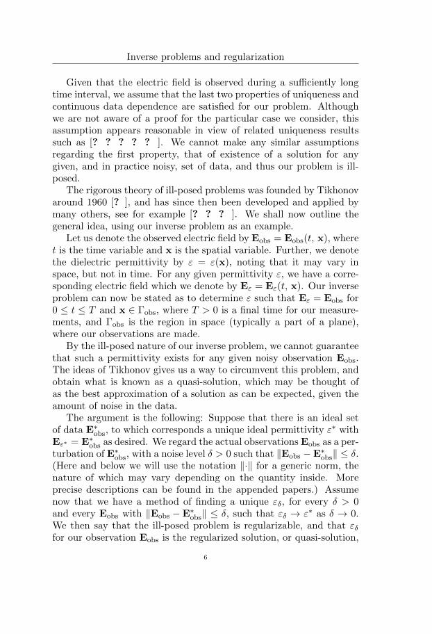
Given that the electric field is observed during a sufficiently longtime interval, we assume that the last two properties of uniqueness andcontinuous data dependence are satisfied for our problem. Althoughwe are not aware of a proof for the particular case we consider, thisassumption appears reasonable in view of related uniqueness resultssuch as [? ? ? ? ? ]. We cannot make any similar assumptionsregarding the first property, that of existence of a solution for anygiven, and in practice noisy, set of data, and thus our problem is ill-posed.

The rigorous theory of ill-posed problems was founded by Tikhonovaround 1960 [? ], and has since then been developed and applied bymany others, see for example [? ? ? ]. We shall now outline thegeneral idea, using our inverse problem as an example.

Let us denote the observed electric field by Eobs = Eobs(t, x), wheret is the time variable and x is the spatial variable. Further, we denotethe dielectric permittivity by ε = ε(x), noting that it may vary inspace, but not in time. For any given permittivity ε, we have a corre-sponding electric field which we denote by Eε = Eε(t, x). Our inverseproblem can now be stated as to determine ε such that Eε = Eobs for0 ≤ t ≤ T and x ∈ Γobs, where T > 0 is a final time for our measure-ments, and Γobs is the region in space (typically a part of a plane),where our observations are made.

By the ill-posed nature of our inverse problem, we cannot guaranteethat such a permittivity exists for any given noisy observation Eobs.The ideas of Tikhonov gives us a way to circumvent this problem, andobtain what is known as a quasi-solution, which may be thought ofas the best approximation of a solution as can be expected, given theamount of noise in the data.

The argument is the following: Suppose that there is an ideal setof data E∗obs, to which corresponds a unique ideal permittivity ε∗ withEε∗ = E∗obs as desired. We regard the actual observations Eobs as a per-turbation of E∗obs, with a noise level δ > 0 such that ‖Eobs −E∗obs‖ ≤ δ.(Here and below we will use the notation ‖·‖ for a generic norm, thenature of which may vary depending on the quantity inside. Moreprecise descriptions can be found in the appended papers.) Assumenow that we have a method of finding a unique εδ, for every δ > 0and every Eobs with ‖Eobs −E∗obs‖ ≤ δ, such that εδ → ε∗ as δ → 0.We then say that the ill-posed problem is regularizable, and that εδfor our observation Eobs is the regularized solution, or quasi-solution,

6


to the problem. It should be noted that we do not require preciseknowledge of ε∗ and E∗obs. The existence of such a pair of ideal dataand solution is an abstract assumption. Only the noise level δ and theactual observations Eobs are needed to obtain εδ.

In addition, Tikhonov proposed a method of constructing εδ forregularizable ill-posed problems, via the minimization of the Tikhonovfunctional, here

(2.1) Fα(ε) :=1

2‖Eε −Eobs‖2 +

α

2‖ε− ε0‖2 ,

where α = α(δ) > 0 is a regularization parameter which should beselected appropriately, in particular we must have α(δ)→ 0 as δ → 0,and ε0 is an initial approximation of ε∗. We will discuss the choiceof α and ε0 further below. Given appropriate choices of α and ε0, aunique minimizer εα of Fα exists, and we can define εδ := εα(δ).

2.1. Choice of regularization parameter. For the theory ofregularization by Tikhonov’s method, it is important to define the cor-rect behaviour of the regularization parameter α = α(δ) as the noiselevel δ tends to zero. In a practical setting however, we cannot con-trol the noise level, but instead we are given fixed data, having somefixed noise level. Thus, how to choose a good value of the regular-ization parameter for a given observation becomes another importantquestion.

Numerous methods for doing so exist, ranging from pure heuristicsto rigorous algorithms. Some examples are the discrepancy principle[? ], the L-curve method [? ], iterative regularization by regarding theregularization parameter as an additional variable in the minimization[? ], and manual choice. See for instance also [? ? ] for additionalexamples. Some of these methods require the Tikhonov functional tobe minimized for several different values of the regularization parame-ter. In our case, minimizing the Tikhonov functional is very expensivein terms of computations, as we will see below. This makes methodswhich calls for repeated minimizations inappropriate for our purposes.

Of other methods, we have considered manual choice, and iterativeregularization. The details are presented in Paper V, where we presenta comparison, from which we conclude that the choice of regulariza-tion parameter does not appear to be the most critical factor in ourapproach to the inverse scattering problem under consideration.

7


2.2. Construction of initial approximation. Not only shouldwe determine an appropriate value of the regularization parameter,we must also find a suitable initial approximation ε0 for the dielectricpermittivity. From the theoretical point of view, any ε0 will do as welet the noise level drop to zero and choose regularization parameteraccordingly. But, again, in practice, we cannot let the noise level dropto zero, and so the choice of ε0 matters for the concrete reconstruction.

The simplest meaningful choice would be to assume that ε0 is con-stant, with a value corresponding to that of the background medium.In absence of any other information, any other choice would requireadditional justification, and so the constant background initial approx-imation is commonly used. This is the case in Papers IV, and V. How-ever, at the cost of performing additional computations, it is possibleto use the observed data to construct a better initial approximation.In Papers I and II, this has been done using a so-called approximatelyglobally convergent method. The full exposition of this method canbe found in the book [? ], and a brief overview is presented in Pa-per II of this thesis. For this introduction, we shall restrict ourselvesto summarizing the key points of this method, in particular as appliedto the construction of an initial approximation for the problem studiedin this thesis.

The method is originally derived for reconstruction of the wavespeed in the acoustic wave equation. It does not rely on any optimiza-tion algorithm, but uses the structure of the differential operator toobtain a sequence of approximations of the wave speed. The elementsof this sequence are computed successively, with the first element com-puted from only the problem domain and the observed data.

In the framework of scalar waves, it can be shown that this sequencecan be constructed in such a way that the elements converge to a wavespeed which is close to, but not necessarily equal to, the ideal wavespeed in Tikhonov’s concept for the reconstruction problem [? ? ].It is from this property the method derives its name. In addition,for correct choice of the regularization parameter, it can be shownthat the corresponding Tikhonov functional is strongly convex in aneighbourhood of the obtained initial approximation, and that thisneighbourhood contains the minimizer (Theorem 3.1 of [? ]).

These important properties are theoretically and numerically es-tablished for reconstruction of speeds of scalar waves. For electromag-netic waves, where the dielectric permittivity ε corresponds to the wave

8

Modelling of the electric field

speed in the scalar case, the dependence of the electric field Eε upon εis more complicated than the dependence of a scalar wave on the wavespeed. Hence, for electromagnetic waves, the approximately globallyconvergent method remains a heuristic, and the techniques used in thecase of scalar waves cannot be used to derive a corresponding versionof the approximately globally convergent method for electromagneticwaves. However, in view of numerical results in the appended papers,we will assume that the strong convexity property holds for Fα withthe initial approximation ε0 obtained as discussed in this section.

3. Modelling of the electric field

Although Tikhonov’s method presented in Section 2, with the aidof the approximately globally convergent method presented in Sec-tion 2.2, shows us the way to proceed with the inverse scattering prob-lem, we are by no means ready yet. In order to minimize the Tikhonovfunctional Fα of (2.1), we need at the very least to be able to evaluateit, and its gradient. This is where the proper mathematical model forthe scattering comes into play. We recall that, in the approximatelyglobally convergent method, the scalar wave equation was employedfor this purpose. This equation is too unsophisticated to truly capturethe nature of electromagnetic waves, though, and instead we shouldresort to Maxwell’s equations

(3.1)

µ∂H

∂t+∇×E = 0,

ε∂E

∂t−∇×H = −σE,

∇ · (εE) = ρ,

∇ · (µH) = 0,

where E = E(x, t) and H = H(x, t) are electric and magnetizingfields, respectively, µ = µ(x) is magnetic permeability, ε = ε(x) isdielectric permittivity as before, σ = σ(x) is conductivity, and ρ =ρ(x, t) is charge density. Here, and for the remaining part of thisintroduction, x ∈ R3 denotes the spatial coordinates, and t > 0 denotesthe time variable.

In contrast to the wave equation model used in the approximatelyglobally convergent method, this full system of Maxwell’s equations,involving six unknown functions (three components each of the two

9


unknown fields E and H), may be too complicated and hence imprac-tical for our computations. Therefore, we observe that we are, for thetime being, concerned with non-magnetic and non-conductive mediain absence of free charges, allowing us to put µ ≡ 1, σ ≡ ρ ≡ 0, and atthe cost of taking additional derivatives obtain the following systemfor E,

(3.2)

ε∂2E

∂t2+∇× (∇×E) = 0 in R3 × (0, T ],

∇ · (εE) = 0 in R3 × (0, T ],

E(·, 0) = 0,∂E

∂t(·, 0) = Iδ(· − x0) in R3,

which we here present as an “ideal” model, set in the whole spaceR3, and for the relevant time interval [0, T ], completed with initialconditions describing a pulse, parallel to I, emanating at the pointx0 ∈ R3 at time t = 0. Here, δ is the Dirac delta.

The system (3.2) is an ideal model in the sense that it captures moreof the physical nature of electromagnetic waves, while it avoids toomuch complexity by not including any quantities which are not directlyrelated to what we measure or seek to image. However, we cannotsolve the system explicitly unless the permittivity ε is very simple,for instance constant. Moreover, being set in the whole space R3, thesystem does not easily lend itself well to numerical approximation byconventional methods. Thus, in order to proceed, we need to truncatethe computational domain.

Suppose that the region of interest, that is, the region where we inthe end will reconstruct the permittivity ε, is contained in a bounded– and for simplicity we may assume rectangular, hence convex – do-main Ω ⊂ R3, such that the permittivity has a constant backgroundvalue close to the boundary as well as outside of Ω, and x0 6∈ Ω. Theconstant background value of the permittivity close to the boundary,together with the divergence condition, implies that the first equationof (3.2) decouples into three independent wave equations in that re-gion. This fact helps us to make sense of the boundary conditions weapply, and we will also take advantage of it in our numerical scheme(see Subsection 4.2).

We describe the systems (3.2) in Ω by adding boundary conditionswhich emulate the free space around Ω, and the initial pulse, whichby the time it reaches Ω is approximated by a plane wave. We end up

10


with the following system:

(3.3)

ε∂2E

∂t2+∇× (∇×E) = 0 in Ω× (0, T ],

∇ · (εE) = 0 in Ω× (0, T ],

∂E

∂n= 0 on ΓN × (0, T ],

∂E

∂n= −∂E

∂ton ΓA × (0, T ],

E = p on ΓI × (0, t1),

∂E

∂n= −∂E

∂ton ΓI × [t1, T ],

E(·, 0) =∂E

∂t(·, 0) = 0 in Ω,

where n denotes the outward unit normal vector on the boundaryΓ = ΓN ∪ ΓA ∪ ΓI of Ω.

The boundary conditions, equations three through six in system(3.3) should be explained in some detail. See also Figure 2 for illus-tration. On ΓN, which correspond to the faces of Ω which are notintersected by the line through the center of Ω and the point x0, weprescribe homogeneous Neumann boundary conditions to simulate freespace stretching away in the directions perpendicular to the incidentplane wave. On ΓA, at the “back” of Ω from the point x0, we prescribethe first order absorbing boundary conditions of Engquist and Majda[? ], to absorb transmitted signals. Finally, on ΓI we prescribe an inci-dent plane wave of profile p = p(t) simulating the signal generated bythe initial pulse in (3.2) far from the source at x0, until it has passedat time t = t1 for some t1 ∈ (0, T ), whence we switch to absorbingboundary conditions to absorb reflected signals.

The model (3.3) is the one that we actually use in computations,with the domain decomposition finite element-finite difference methodof [? ] for discretization. We shall return to this method below. Be-fore we close this section, in order to simplify further presentation, weintroduce a reduced version of (3.3), with simplified boundary condi-tions on a shrunken domain Ω. We also incorporate the divergencecondition, the second equation of (3.3), as stabilization term of theform −s∇(∇ · (εE)), to the left hand side of the first equation, see [?

11


Ω

Γ ΓΓ

Ω

x0

N A I

x0

Figure 2. Schematic illustration of the truncatedcomputational domain Ω (upper left), its boundaryconsisting of three parts Γ = ΓN ∪ ΓA ∪ ΓI (lower left),and viewed from above with incident approximatelyplane wave (right).

? ]. We choose s = 1 since this facilitates the derivation of the numer-ical scheme, and that is the value we typically use in computations.The stabilization term does not change the solution of the problem,but induces stability in the numerical approximation scheme which willbe outlined in Section 4 (see [? ]). It should also be mentioned thatthis numerical scheme may produce convergence to the wrong resultin the case of non-convex domains, but this problem does not occurhere, since we may always assume that Ω is convex in our problemframework.

(3.4)

ε∂2E

∂t2+∇× (∇×E)−∇(∇ · (εE)) = 0 in Ω× (0, T ],

∂E

∂n= P on Γ× (0, T ],

E(·, 0) =∂E

∂t(·, 0) = 0 in Ω.

12

Finite element approximation

Here P = P(x, t) is a given function defined on the entire Γ× (0, T ].

4. Finite element approximation

With the models (3.3) as well as (3.4), we no longer face the prob-lem of dealing with an infinite spatial domain which was the case in(3.2). But, there are still no explicit formulas available for the solu-tion Eε for a given ε, except in some trivial cases. Hence, we mustconsider numerical approximations. Our main approximation schemeis the finite element method (in fact hybridized with a finite differencescheme, as we will return to at the end of this section) which we out-line below. In this section, we will illustrate this method as applied tothe system (3.4), for good overviews, we recommend [? ? ? ? ? ].

The idea of this method is the following: First, we should refor-mulate the original problem in variational form. This form makes theproblem easier to analyze than it was in the original form, and onecan show that the solutions to the two formulations coincide, undersuitable assumptions on the problem domain and the data. The varia-tional form is, in principle, no easier to actually solve than the originalform, but it shows a way to proceed systematically with constructingapproximations to the solution. The way to do it is to restrict the orig-inal function space over which the variational formulation was statedto a finite-dimensional subspace consisting of simple functions. Thus,we obtain a finite approximate problem, the finite element formula-tion. This problem can be solved systematically (with a computer),but the solution is no longer the same as to the original or variationalproblem, except in trivial cases. However, by selecting the finite di-mensional subspace appropriately, we can assure that the solutions areclose to each other, and that they become even closer if we increasethe dimension of the finite-dimensional subspace.

For an example, let us consider the problem (3.4). To elaborate, weshould really state it in the following way: Given a permittivity ε in aset U ε of admissible permittivities, and a function P ∈ C(Γ× [0, T ]),determine a function E ∈ C2(Ω× [0, T ]; R3), such that these functionssatisfy (3.4).

The set U ε is described in detail in for instance Paper IV. Here wemerely note that we should have ε continuous, positive, bounded fromabove and below, and constantly equal to 1 on Γ. We have used thenotation Ck(X; Y ) for k times continuously differentiable functions

13


over the domain X taking values in the space Y , leaving out k if it iszero and Y if it is R.

Whether or not the function spaces stated in this problem are theleast restrictive ones, and whether the problem is well posed in thisformulation can be analyzed, but such analysis is beyond the scopeof this thesis. Instead we refer to, for example, [? ? ], and assumefor the time being that a solution does exist, and for this solution, wemultiply the first equation of (3.4) by a smooth R3-valued function φdefined in Ω× [0, T ], and integrate. This gives∫ T

0

∫Ωε(x)

∂2E

∂t2(x, t) · φ(x, t) dx dt

+

∫ T

0

∫Ω∇× (∇×E(x, t)) · φ(x, t) dx dt

−∫ T

0

∫Ω∇(∇ · (ε(x)E(x, t))) · φ(x, t) dx dt = 0.

Seeing that these expressions tend to become long and bulky, it is ap-propriate to simplify the notation by introducing the L2-inner product:

〈u, v〉X :=∫X(u, v),

where (·, ·) denotes the standard inner product on Rn, for appropriaten ∈ N, and the integral is with respect to Lebesgue measure on X.This allows us to rewrite the above equation as

(4.1) 〈ε∂2E∂t2

, φ〉ΩT + 〈∇ × (∇×E), φ〉ΩT − 〈∇(∇ · (εE)), φ〉ΩT = 0

with ΩT := Ω× (0, T ).We proceed to write this identity in a more symmetric form, and

lower the burden of derivatives on a single function, by applying thefollowing integration by parts formulas∫ T

0u′(t)v(t) dt+

∫ T

0u(t)v′(t) dt = u(T )v(T )− u(0)v(0),∫

Ω∇u(x) · v(x) dx +

∫Ωu(x)∇ · v(x) dx =

∫Γu(x)n · v(x) dS

14


and the identity ∇× (∇×u) = −∆u+∇(∇·u). Using these formulasin (4.1) we get

− 〈ε∂E∂t ,∂φ∂t 〉ΩT + 〈ε∂E∂t (·, T ), φ(·, T )〉Ω − 〈ε∂E∂t (·, 0), φ(·, 0)〉Ω

+ 〈∇E, ∇φ〉ΩT − 〈∂E∂n , φ〉ΓT − 〈∇ ·E, ∇ · φ〉ΩT + 〈∇ ·E, n · φ〉ΓT+ 〈∇ · (εE), ∇ · φ〉ΩT − 〈∇ · (εE), n · φ〉ΓT = 0,

with ΓT := Γ× (0, T ).Here we observe that ∂E

∂n = P and ε ≡ 1 on Γ, that ∂E∂t (·, 0) ≡ 0,

and prescribe φ(·, T ) ≡ 0 to arrive at

(4.2)− 〈ε∂E∂t ,

∂φ∂t 〉ΩT + 〈∇E, ∇φ〉ΩT

− 〈∇ ·E, ∇ · φ〉ΩT + 〈∇ · (εE), ∇ · φ〉ΩT − 〈P, φ〉ΓT = 0.

We now pause to make some observations. For equation (4.2) tomake sense, we do not really have to impose such strong restrictionson E, P, and φ as we originally did. It is enough to have at most onederivative in either space or time on either of E and φ, and none of thefunctions need to be pointwise defined, as long as the integrals are welldefined. Strictly speaking, this means that they need not be functionsat all, but for convenience, we will continue to refer to them as such.In fact, it is enough to have E, φ ∈ H1(ΩT ; R3) and P ∈ L2(ΓT ; R3),where

L2(ΓT ; R3) := u : ΓT → R3 : ‖u‖ΓT <∞,H1(ΩT ; R3) := u : ΩT → R3 : ‖u‖ΩT , ‖∇u‖ΩT ,

∥∥∂u∂t

∥∥ΩT

<∞

with ‖·‖X :=√〈·, ·〉X , and the derivatives are understood in the weak

sense. That is, ∂u∂t is defined by the relation

〈∂u∂t , φ〉ΩT = −〈u, ∂φ∂t 〉ΩTfor all φ ∈ C∞(ΩT ; R3) with compact support in ΩT , that is, vanishingfor x close to Γ and t close to 0 and T . Similar relations define ∇u,∇× u, and so on.

Putting what we have done so far together leads us to the fol-lowing variational formulation of the problem 3.4: Given a permit-tivity ε ∈ U ε, and a function P ∈ L2(ΓT ; R3), determine a functionE ∈ H1(ΩT ; R3) such that E(·, 0) ≡ 0 and (4.2) is satisfied for thesefunctions and all φ ∈ H1(ΩT ; R3) with φ(·, T ) ≡ 0.

15


Again, careful analysis may show that, for instance, the assumptionP ∈ L2(ΓT ; R3) is stronger than strictly necessary, but this assumptionis sufficient for our purposes here.

The variational formulation enables us to analyze the problem eas-ier in the framework of functional analysis, but it does not in itselftell us how to actually compute a solution. By making a finite di-mensional approximation, we obtain a problem for which is relativelystraight-forward to compute the solution, but this solution is then onlyan approximation to solution of the variational problem.

We will concentrate on approximation in the space H1(ΩT ; R3)since we consider P ∈ L2(ΓT ; R3) to be known exactly. Our aim is toconstruct a subspace of simple functions, which can approximate anyfunction in H1(ΩT ; R3), and for which we can easily find a basis whichwill allow us to reduce the variational problem, restricted to the finitedimensional subspace, to a problem of linear algebra.

Most methods for constructing such a subspace are based on divid-ing the underlying space, in our case ΩT into small subregions – cells– and prescribe that the functions of the subspace should belong tosome simple class on each cell. In the computations reported in theappended papers of this thesis, we have used polynomials of degree oneon each cell, as we will shortly detail. The main reason for this is thatthe obtained space will allow domain decomposition and hybridiza-tion with the simpler but less flexible finite difference method in themanner of [? ]. Polynomials of higher or lower degrees are also com-monly used, as are special classes of polynomials or functions, such asin the edge element method of Nedelec [? ? ], which is widely used forMaxwell’s equations and related systems. Those polynomials removethe need of a stabilization term, but is not as clear how to constructa domain decomposition method similar to [? ] for the correspond-ing finite element method and a finite difference method. There arealso certain methods which do not rely (directly) on a division of theproblem domain into cells, such as radial basis function methods [?], or extended finite element methods [? ], but these methods oftenproduce less well-conditioned systems of equations than the cell-basedmethods, hence we do not consider such methods here.

To begin with the actual construction of finite dimensional sub-spaces, we let Th = K be a division of Ω into tetrahedra K. This di-vision is associated to a mesh function h = h(x) with h(x) := diam(K),x ∈ K, where diam(K) is the diameter, the largest distance between

16


two points, of K. We also partition [0, T ] uniformly into subinter-vals Iτ := Ik with Ik = [tk+1, tk], k = 0, . . . , Nτ , for 0 = t0 <. . . < tNτ = T where tk+1 − tk = τ := T/Nτ . We choose Nτ suchthat τ ∝ minx∈Ω h(x) to fulfil a so-called Courant-Friedrichs-Lewycondition [? ], which ensures stability of the numerical scheme we areconstructing.

We now define the subspace Sh as the space of those functions inH1(ΩT ; R3) which on each tetrahedron K and each time interval Ikare described by an R3-valued polynomial of degree one in the spatialvariable, times a scalar polynomial of the time variable. In other words,

Sh := u ∈ H1(ΩT ; R3) : u|K×Ik ∈ P 1(K; R3)× P 1(Ik)

∀K ∈ Th, Ik ∈ Iτ,where

P 1(K; R3) := u ∈ C(K; R3) : u(x) = Ax + b, A ∈ R3×3, b ∈ R3,P 1(Ik) := u ∈ C(Ik) : u(t) = at+ b, a, b ∈ R.

The approximation properties of such a subspace is reflected in thetypical interpolation error estimate

‖u− ihu‖ΩT ≤ C ‖hmDmu‖ΩT

where ih : H1(ΩT ; R3)→ Sh is an appropriate interpolation operator,such as the Scott-Zhang interpolant [? ], and Dm denotes derivativesof order m. Thus, in the worst case, the interpolation error decreaseslinearly (m = 1) with the mesh size, for u ∈ H1(ΩT ; R3). Interpolationestimates like these play an important role in error analysis for finiteelement methods, which we will see examples of below.

We can now state the finite element formulation of the problem justas we stated the variational formulation, except that we replace thespace H1(ΩT ; R3) by its subspace Sh. That is: Given ε ∈ U ε, and afunction P ∈ L2(ΓT ; R3), determine Eh ∈ Sh with Eh(·, 0) ≡ 0, suchthat (4.2) holds for Eh and for all φ ∈ Sh with φ(·, T ) ≡ 0. (Notethat this formulation does not rely on our explicit choice of Sh, andwould be valid for other subspaces if required.)

By introducing a basis for Sh, we can reduce this finite elementformulation to a system of linear algebraic equations. For a basis, thereis a straight-forward choice, which yields good numerical properties.

The basis is constructed as follows: Let xiNhi=1 be the set of nodes on

17


Th and for i = 1, . . . , Nh define ϕi = ϕi(x) by

ϕi|K ∈ P 1(K) := a · x + b, a ∈ R3, b ∈ R3 ∀K ∈ Th,

ϕi(xj) := δi, j :=

1, i = j,

0, i 6= j,j = 1, . . . , Nh.

Similarly, we define χk = χk(t) for k = 0, . . . , Nτ by

χk|Il ∈ P 1(Il) ∀Il ∈ Iτ ,χk(tl) = δk, l, l = 0, . . . , Nτ .

It is now easy to verify that emϕiχk, where e1, e2, e3 is thestandard basis for R3, is a basis for Sh. This means that we mayexpand

Eh(t, x) =3∑

n=1

Nh∑j=1

Nτ∑l=1

Ej, ln enϕj(x)χl(t),

where Ej, ln are the weights that we seek. Moreover, it is sufficientto use φ = emϕiχk for m = 1, 2, 3, i = 1, . . . , Nh, k = 0, . . . , Nτ − 1in the finite element formulation.

By doing so, we reduce the finite element formulation for (4.2) tothe following system of linear equations

(4.3) A(ε)Ek+1 − 2Ek + Ek−1

τ2+B(ε)

Ek+1 + 4Ek + Ek−1

6= τ2Pk,

for k = 1, . . . , Nτ − 1, with the slightly modified system

(4.4) A(ε)Ek+1 −Ek

τ2+B(ε)

Ek+1 + 2Ek

6= τ2Pk,

for k = 0. Here A(ε) and B(ε) are matrices defined by

A(ε) :=

M(ε) 0 00 M(ε) 00 0 M(ε)

,B(ε) :=

S +D1, 1(ε) D1, 2(ε) D1, 3(ε)D2, 1(ε) S +D2, 2(ε) D2, 3(ε)D3, 1(ε) D3, 2(ε) S +D3, 3(ε)

,M(ε) := (mi, j(ε)) := (

∫Ω ε(x)ϕj(x)ϕi(x) dx),

S := (∫

Ω∇ϕj(x) · ∇ϕi(x) dx)

Dm,n(ε) := (∫

Ω∇ · ((ε(x)− 1)ϕj(x)en)∇ · (ϕi(x)em) dx),

18


and

Ek :=

Ek1

Ek2

Ek3

, Ekm :=

E1, km...

ENh, km

, E0 = 0,

Pk :=

Pk1

Pk2

Pk3

, Pkm :=

p1, km...

pNh, km

,pi, km :=

∫ΓT

Pm(t, x)ϕi(x)χk(t) dS dt.

Thus, if we are given ε and P, we can compute the matrices A(ε)and B(ε), as well as the vectors Pk, and hence compute the vectors Ek,k = 1, . . . , Nτ by (4.3) and (4.4), starting from the known E0 = 0. Wealso note that one particular advantage of the basis we used is thatthe matrices M(ε), S, and Dm,n(ε) become sparse and structured,symmetric in the case of M(ε) and S, since any two basis functionsϕi and ϕj overlap only if the nodes xi and xj are adjacent, otherwisethe product of the basis functions, or their derivatives, are zero in allof Ω.

Although the system (4.3) is sparse, solving it repeatedly for eachtime step may be very time consuming, especially since we eventuallycompute the electric field not once but several times when solving theinverse problem. There are ways to circumvent this, and in our work wehave considered the following two: making additional approximationsto obtain an explicit formula for Ek+1 in terms of Ek and Ek−1, andusing parallel computations. For the former, we use so-called masslumping [? ], approximating

A(ε) ≈ AL(ε) :=

ML(ε) 0 00 ML(ε) 00 0 ML(ε)

where ML(ε) is diagonal, with the row-sums of M(ε) as diagonal en-tries, and

Ek+1 + 4Ek + Ek−1

6≈ Ek.

With these approximations, we get

Ek+1 = 2Ek −Ek−1 + τ2AL(ε)−1(Pk −B(ε)Ek),

19


which is explicit, since the inverse of the diagonal matrix AL(ε) is justanother diagonal matrix, with reciprocal diagonal entries.

For parallel computations, the idea of which is to divide the fullproblem into smaller sub-problems which are solved in parallel on sev-eral computer processors, we use the PETSc library [? ] as imple-mented in the software package WavES [? ].

4.1. Adaptivity. Regardless of the practicalities of the imple-mentation, having stated a variational problem and its correspondingfinite element formulation, where the solution to the latter approxi-mates the solution to the former, leads to two natural questions:

(1) How large is the error, the difference between the finite ele-ment solution which we compute, and the solution to the vari-ational problem, which we ideally would like to have? And,

(2) how do we efficiently make this error as small as we require?

The first of these two questions is answered through a priori erroranalysis. In such analysis, one relates the error to the mesh size h andthe problem data (Ω, T , ε, and P for the problem above). Typical re-sults show how the error decreases as some power of h, with a constantrelated to the data, as h tends to zero.

In answering the second question, that of efficiently reducing theerror, another kind of analysis, a posteriori error analysis, plays animportant role. Here, the idea is to estimate local (in space or time)contributions to the error, in terms of quantities which are actuallycomputed, such as Eh in the problem described above. Since theapproach we use to the inverse problem is based on improving theaccuracy of an initial approximation, a posteriori error analysis is ofprimary interest. In the remainder of this section, we will describethe principle of how to use such analysis to efficiently reduce errors,with so-called adaptive error control (see for instance [? ? ]). For theprecise estimates we use, we refer to the next section as well as theappended papers, in particular Paper IV.

To illustrate the principle, suppose that we have a mesh Th as above,and that we on this mesh have computed a quantity qh, approximatingthe true quantity q. Suppose also that through a posteriori error anal-ysis, we have obtained an estimate on the form ‖q − qh‖ ≤ C ‖Rh, qh‖,where C > 0 is some constant, and Rh, qh = Rh, qh(x) is some knownnon-negative function, depending only on the listed computed quanti-ties, such that, in the worst case |q(x)− qh(x)| ≈ CRh, qh(x).

20


The idea is now to use a balancing principle, reducing large contri-butions to the error while not wasting additional computational effortson reducing errors which already are small. Thus, as we have boundedthe error in terms of Rh, qh , and as we know that a finer mesh (withsmaller mesh size h) leads to a smaller error, our strategy for reducingthe error is to make the mesh finer where Rh, qh is close to attaining itsmaximum value. In other words, we have the following step by stepprocedure:

0: Make an initial coarse mesh Th.1: Compute qh on the current mesh Th.2: Compute Rh, qh on the current mesh, using qh from Step 1.3: Check some stopping criterion, such as the size of Rh, qh , if

the criterion is satisfied, stop computing and accept the latestapproximation qh, otherwise proceed to Step 4.

4: Refine the current mesh by splitting cells in which Rh, qh(x) ≥θmaxxRh, qh(x), where θ ∈ (0, 1) is a chosen tolerance. Thenreturn to Step 1 with the refined mesh as the current mesh.

We illustrate one cycle of this procedure schematically for a meshin one dimension in Figure 3.

4.2. Hybridization with finite differences. We conclude thissection with some words about the hybridization of the finite elementmethod with the finite difference method, which was mentioned pre-viously. The details can be found in [? ]. Here, we begin with a briefintroduction to the finite difference method.

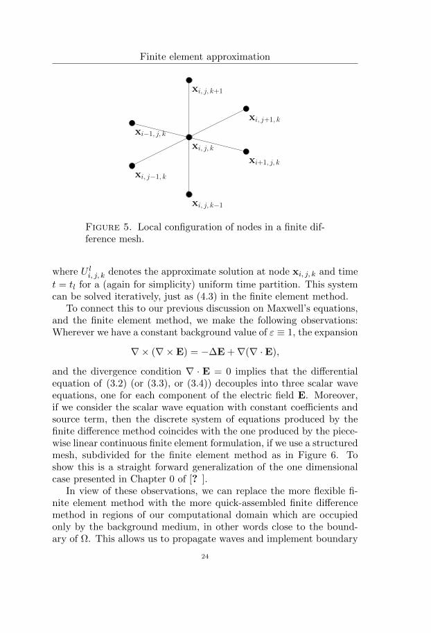
As with the finite element method, we start with a subdivisionof the problem domain. Here, however, we are not concerned withwhat happens inside cells, but focus on the nodes from the beginning.As a consequence, we must be more restrictive with what types ofsubdivisions that we allow, namely, we require that the subdivisionproduces a rectangular grid of nodes (see Figure 4).

On this rectangular grid, we approximate the differential equationat each node using difference quotients for the derivatives. For exam-ple, if we consider the scalar wave equation

∂2u

∂t2(x, t)−∆u(x, t) = 0,

we get the following equation at each node xi j k (see Figure 5)

21


(0) (1)

(2) (3)

Figure 3. One dimensional schematic illustration ofadaptivity: (0) The mesh at the start of the cycle.(1) The mesh with computed approximation. (2) Es-timated errors, indicated by the width of the gray boxaround the approximation. (3) The refined mesh, for acertain tolerance.

∂2Ui, j, k(t)

∂t2+Ui−1, j, k(t)− 2Ui, j, k(t) + Ui+1, j, k(t)

h2

+Ui, j−1, k(t)− 2Ui, j, k(t) + Ui, j+1, k(t)

h2

+Ui, j, k−1(t)− 2Ui, j, k(t) + Ui, j, k+1(t)

h2= 0,

where Ui, j, k(t) denotes the nodal value of the approximation of thesolution at node xi, j, k time t, and h is the distance between two adja-cent nodes, assumed for simplicity to be constant. It is convenient todenote the last three terms in the left hand side of the above equationby −∆hUi, j, k(t).

22


Figure 4. Finite difference meshes (left), and finiteelement meshes (right). The meshes in the upper parthave the same 36 nodes. The lower figures show themeshes adaptively refined to fit the lighter circle to ap-proximately the same accuracy. Then the finite differ-ence mesh has 100 nodes, while the finite element meshhas 56 nodes.

Making a similar discretization in the time variable, we finally ob-tain

−U l+1i, j, k + 2U li, j, k − U l−1

i, j, k

τ2−

∆hUl+1i, j, k + 4∆hU

li, j, k + ∆hU

l−1i, j, k

6= 0,

23


xi, j, k

xi, j, k+1

xi, j, k−1

xi−1, j, k

xi+1, j, k

xi, j+1, k

xi, j−1, k

Figure 5. Local configuration of nodes in a finite dif-ference mesh.

where U li, j, k denotes the approximate solution at node xi, j, k and time

t = tl for a (again for simplicity) uniform time partition. This systemcan be solved iteratively, just as (4.3) in the finite element method.

To connect this to our previous discussion on Maxwell’s equations,and the finite element method, we make the following observations:Wherever we have a constant background value of ε ≡ 1, the expansion

∇× (∇×E) = −∆E +∇(∇ ·E),

and the divergence condition ∇ · E = 0 implies that the differentialequation of (3.2) (or (3.3), or (3.4)) decouples into three scalar waveequations, one for each component of the electric field E. Moreover,if we consider the scalar wave equation with constant coefficients andsource term, then the discrete system of equations produced by thefinite difference method coincides with the one produced by the piece-wise linear continuous finite element formulation, if we use a structuredmesh, subdivided for the finite element method as in Figure 6. Toshow this is a straight forward generalization of the one dimensionalcase presented in Chapter 0 of [? ].

In view of these observations, we can replace the more flexible fi-nite element method with the more quick-assembled finite differencemethod in regions of our computational domain which are occupiedonly by the background medium, in other words close to the bound-ary of Ω. This allows us to propagate waves and implement boundary

24

Minimization, the Lagrangian approach

x1

x2

x3

x4

x5

x6

x7

8x

Figure 6. A subdivision of a cube with nodes xi,i = 1, . . . , 8, into six tetrahedra 41254, 41345, 42465,43457, 44586, 44578, where the tetrahedron 4ijkl hasnodes xi, xj , xk, and xl.

conditions more efficiently, while maintaining flexibility to describecomplicated variations in the dielectric permittivity.

5. Minimization, the Lagrangian approach

We have now presented methods for obtaining an initial approxima-tion, and for approximately solving the direct problem of computingthe electric field. Thus we can construct and evaluate the Tikhonovfunctional (2.1), and we may turn to the actual minimization.

As a continuous optimization problem, we expect this method torequire the computation of gradients in order to achieve good ratesof convergence in any iterative method used to solve it. Comput-ing any kind of gradient of the Tikhonov functional directly is a verycomplicated task, however, since its dependence on the permittivityis implicit through the solution of a partial differential equation. Us-ing techniques of optimal control theory presented in [? ], we cancircumvent this difficulty.

With this approach, we first reformulate the minimization problemas a problem of two formally independent variables, where a constraintensures the correct dependence. That is, we consider the problem to

25


minimize

Fα(ε, E) :=1

2‖E−Eobs‖2ΓT +

α

2‖ε− ε0‖2Ω

for ε ∈ U ε, E ∈ H1(ΩT ; R3), E(·, 0) ≡ 0, under the constraint that

D(ε, E, φ) = 0 ∀φ ∈ H1(ΩT ; R3) : φ(·, T ) ≡ 0,

where D is the functional of the variational formulation of the directproblem.

We may solve this problem by determining the stationary point tothe corresponding Lagrangian

L(ε, E, λ) := Fα(ε, E, λ) +D(ε, E, λ).

Since the three variables of the Lagrangian may be varied indepen-dently, calculating derivatives of the Lagrangian is much more straightforward than doing so for the Tikhonov functional. Indeed, we find thepartial Frechet derivatives of L, acting on ε ∈ U ε, E ∈ H1(ΩT ; R3) :E(·, 0) ≡ 0, and λ ∈ H1(ΩT ; R3) : λ(·, T ) ≡ 0, respectively, to be

∂L

∂ε(ε, E, λ; ε) = α〈ε− ε0, ε〉Ω−〈∂E∂t · ∂λ∂t , ε〉ΩT + 〈∇ · λ, ∇ · (εE)〉ΩT ,

∂L

∂E(ε, E, λ; E) = A(ε, E, λ, E),

∂L

∂λ(ε, E, λ; λ) = D(ε, E, λ),

where A is the functional of a variational formulation of an adjointproblem to the direct problem, where E acts as boundary data.

At the stationary point, all of these partial derivatives are zero, orin other words, their action on each admissible ε, E, and λ is zero.We observe that putting ∂L/∂λ to zero in this manner implies that Esolves the variational form of the direct problem, and putting ∂L/∂Eto zeros implies that λ solves the adjoint variational problem, deter-mined by A. Thus, we can ensure that these two partial derivativesremain zero by letting E and λ solve the correct variational problems,or in practice, the corresponding finite element problems.

Unlike the case of ∂L/∂E = 0 and ∂L/∂λ = 0, there is no obviousway to achieve ∂L/∂ε = 0 by solving a system of partial differentialequations, and so we instead apply the conjugate gradient method.We then arrive at the following algorithm:

26


0. Let ε0 be the initial approximation for the permittivity, setL2(Ω) 3 d−1 = 0, and let k = 0.

1. Compute Ek by solving D(εk, Ek, ·) = 0.2. Compute λk by solving A(εk, Ek, λk, ·) = 0.3. Compute the gradient gk = ∂L

∂ε (εk, Ek, λk).4. Update the permittivity by the conjugate gradient rule:

dk = −gk +‖gk‖2Ω‖gk−1‖2Ω

dk−1,

εk+1 = εk + βkdk

for step size βk > 0 such that(d

dβL(εk + βdk, Ek, λk)

)∣∣∣∣β=βk

= 0.

5. Check stopping criterion. If satisfied, accept the current εk,otherwise increase k by 1 and return to step 1.

In practice, we replace the variational problems of steps 1 and 2of this algorithm by the corresponding finite dimensional problemsover some mesh. Consequently, we also obtain an approximate updateof the permittivity in step 5, and an approximate permittivity εh asoutput.

At this point, we would like to apply the adaptive algorithm ofSection 4.1, with q = ε being the stationary point to the Lagrangian,and qh = εh being the output of the algorithm above. In order todo so, we require an a posteriori error estimate for ε − εh. Such anestimate is derived in Paper IV, and we here outline the main steps ofthe derivation.

As a first step, we use the strong convexity as discussed in Sec-tion 2.2. This implies that there is some constant C > 0 such that

‖ε− εh‖2Ω ≤ C |F ′α(ε; ε− εh)− F ′α(εh; ε− εh)| ,where F ′α(·, ε− εh) denotes the action of the Frechet derivative of Fαon ε− εh. Since ε minimizes Fα, the first term in the right hand sidevanishes, leaving us with

‖ε− εh‖2Ω ≤ C |F ′α(εh; ε− εh)| .We can relate this derivative of Fα to ∂L/∂ε to get

‖ε− εh‖2Ω ≤ C∣∣∂L∂ε (εh, Eεh , λεh ; ε− εh)

∣∣ ,27


where Eεh and λεh are the exact solutions to the direct and adjointvariational problems, respectively, using the approximate permittivityεh.

A Cauchy-Schwartz inequality argument now gives, after cancella-tion of a common factor ‖ε− εh‖Ω,

‖ε− εh‖Ω ≤ C∥∥∂L∂ε (εh, Eεh , λεh)

∥∥ .Since we cannot evaluate Eεh and λεh , we need some further ma-

nipulations to obtain an a posteriori estimate. We add and subtract∂L∂ε (εh, Eh, λh), where Eh and λh are finite element approximationsof Eεh and λεh , which we have computed on steps 1 and 2 of theminimization algorithm. With the triangle inequality, this gives

(5.1)‖ε− εh‖ ≤ C

∥∥∂L∂ε (εh, Eεh , λεh)− ∂L

∂ε (εh, Eh, λh)∥∥

+ C∥∥∂L∂ε (εh, Eh, λh)

∥∥ .The second term of the right hand side in (5.1) has already been

calculated (up to the constant C) as part of the minimization algo-rithm, while the first term must be estimated further. To this end, welinearize the difference as

∂L

∂ε(εh, Eεh , λεh)− ∂L

∂ε(εh, Eh, λh)

≈ ∂

∂ε

(∂L

∂E(εh, Eh, λh; Eεh −Eh) +

∂L

∂λ(εh, Eh, λh;λεh − λh)

).

Here, we can use the fact that the Frechet derivatives are linear inthe last argument, and the fact that Eh and λh, as solutions to thefinite element problems, are also valid test functions, to replace the lastEh and λh of the two terms above, by the corresponding interpolantsihEεh and ihλh, respectively. Thus we get

∂L

∂ε(εh, Eεh , λεh)− ∂L

∂ε(εh, Eh, λh)

≈ ∂

∂ε

(∂L

∂E(εh, Eh, λh; Eεh − ihEεh)

+∂L

∂λ(εh, Eh, λh;λεh − ihλεh)

).

28

Other methods

Now, we can use the Cauchy-Schwartz inequality and interpolationestimates to get∥∥∂L

∂ε (εh, Eεh , λεh)− ∂L∂ε (εh, Eh, λh)

∥∥≤ Ci

∥∥∥ ∂2L∂ε∂E(εh, Eh, λh)

∥∥∥∥∥∥h [∂Eh∂n

]+ τ

[∂Eh∂t

]∥∥∥+ Ci

∥∥∥ ∂2L∂ε∂λ(εh, Eh, λh)

∥∥∥∥∥∥h [∂λh∂n ]+ τ[∂λh∂t

]∥∥∥ ,where Ci > 0 is an interpolation constant, and [·] denotes jumps ofdiscontinuous functions over faces in the triangulation of the compu-tational domain, and nodes in the time partition.

Putting this last estimate back into (5.1), we obtain the final esti-mate

‖ε− εh‖Ω ≤ CCi

∥∥∥ ∂2L∂ε∂E(εh, Eh, λh)

∥∥∥∥∥∥h [∂Eh∂n

]+ τ

[∂Eh∂t

]∥∥∥+ CCi

∥∥∥ ∂2L∂ε∂λ(εh, Eh, λh)

∥∥∥∥∥∥h [∂λh∂n ]+ τ[∂λh∂t

]∥∥∥+ C

∥∥∂L∂ε (εh, Eh, λh)

∥∥ ,where the first term corresponds to the error incurred by the approx-imation of the electric field, the second term corresponds to the errorincurred by the approximation of the solution to the adjoint problem,and the last term corresponds to the error incurred by the approxima-tions in the computation of the dielectric permittivity.

6. Other methods

We have now presented the principles and ideas of our approach tothe electromagnetic inverse problem. To round off this introductionwe will here perform a brief comparison between the method describedin this thesis, and other methods which are commonly used for solvingrelated inverse problems.

We begin by mentioning methods of boundary maps which arewidely studied in the mathematical community of inverse problems(see for example[? ? ] and many other works by Salo, Somersalo,Uhlmann, and co-workers). These methods usually rely on observa-tions of scattering of several waves, and thus with over-determined in-verse problems which are quite different from the single-measurementcontext that we deal with in this thesis.

In engineering, minimization based approaches – again determinis-tic or stochastic – are more common, also for imaging problems similar

29

Outline of the appended papers

to the one studied here. See for example [? ? ? ? ? ? ]. One ma-jor difference between the typical approach in engineering, and themethod described in this thesis, is that we are dealing with observa-tions and computations in time-domain, while the usual engineeringapproach is set in frequency-domain, that is, in mathematical ter-minology, on the Fourier side in the time variable. This removes theneed of time stepping, but introduces a frequency parametrization andcomplex arithmetic instead. As such, this may or may not make themethod less computationally demanding, depending on the applica-tion. By imposing restrictions and parametrizations of the incidentwaves, and the geometry of the scatterers, one can lower the com-putational complexity significantly, possibly even allowing the use ofanalytical solution formulas, usually in terms of Hankel and Besselfunctions, for the direct problem. Naturally, this restricts the type ofproblems which the method may be applied to. Thus, we can concludethat the method we study in this thesis may be more computation-ally demanding, but is comparatively flexible in terms of geometricalconfiguration of the scatterers and the nature of the incident waves.

7. Outline of the appended papers

Papers I, II, and III were previously included in the licentiate the-sis [? ]. The first two papers demonstrate the performance of ourmethod on experimental data from a laboratory at the University ofNorth Carolina at Charlotte, USA. In Paper I, the data representsscatterers placed in air, while the data in Paper II is for the morechallenging case of scatterers placed inside a box filled with dry sand.Good reconstructions are obtained in both cases, but with restrictionon the depth at which the scatterer was placed below the surface ofthe sand in the studies of Paper II. A case of super-resolution, wheretwo scatterers at a separation of less than one half of a wavelengthwere resolved separately, is observed in Paper II.

Paper III can be regarded as a pre-work to Paper IV, it concernsa simpler a posteriori error estimate, for the error in the value ofthe Lagrangian, L(ε, E, λ) − L(εh, Eh, λh), and introduces an alter-native stabilization term. This stabilization fits into the same gen-eral framework as the one outlined above, namely, we consider a gen-eral stabilization term of the form −∇(s∇ · (εE)), where we requires = s(x) ≥ 1/ε(x) by Theorem 4.1 of [? ]. In this introduction as

30

Outline of the appended papers

well as the remaining appended papers we take a constant s, while inPaper III we take s = 1/ε, which allows us to expand ∇ × (∇ × E)and cancel certain terms (see Paper III for additional details).

In Paper IV, we derive in full detail the a posteriori error estimatewhich was sketched in Section 5, and present additional numericalresults from simulated data for small scatterers with low contrast.

Paper V is devoted to effect of different techniques for choosingthe regularization parameter on the quality of the reconstructed di-electric permittivity. We find that the regularization parameter haslittle impact on the quality of the reconstruction for our inverse prob-lem, and hence other aspects of the reconstruction procedure are moreimportant for future studies.

31

Papers

Paper I

Reprinted from Larisa Beilina, Nguyen Trung Thanh, Michael V. Klibanov

and John Bondestam Malmberg, Reconstruction of shapes and refractive

indices from backscattering experimental data using the adaptivity, Inverse

problems 30:105007, 2014, with permission from the publisher.

Paper II

Reprinted from Larisa Beilina, Nguyen Trung Thanh, Michael V. Klibanov

and John Bondestam Malmberg, Globally convergent and adaptive finite ele-

ment methods in imaging of buried objects from experimental backscattering

radar measurements, Journal of Computational and Applied Mathematics,

289:371–391, 2015 with permission from Elsevier.

Paper III

Reprinted from John Bondestam Malmberg, A posteriori error estimate in

the Lagrangian setting for an inverse problem based on a new formulation of

Maxwell’s system, volume 120 of Springer Proceedings in Mathematics and

Statistics, pages 42–53, Springer, 2015, with permission from the publisher.

Paper IV

John Bondestam Malmberg, and Larisa Beilina. An Adaptive Finite Element

Method in Quantitative Reconstruction of Small Inclusions from Limited

Observations. Manuscript submitted to Applied Mathematics & Information

Sciences.

Paper V

John Bondestam Malmberg, and Larisa Beilina. Iterative Regularization andAdaptivity for an Electromagnetic Coefficient Inverse Problem. Manuscriptto appear in the Proceedings of the 14th International Conference of Numer-ical Analysis and Applied Mathematics.

e cient adaptive algorithms for an electromagnetic coe ... · e cient adaptive algorithms for an...

Documents