Reversibility, irreversibility, Gibbsianity

Dynamics of Ising spin systems

CG&AJ Bray 2009CG 2011CG 2013CG&M Pleimling 2014CG&JM Luck 2014

GG Institute May 26, 2014

with thanks to J Lebowitz

Take flipping rate for 2D square lattice

then stationary state is Boltzmann-Gibbs and detailed balance (w.r.t. Ising energy) satisfied

Künsch 1984:

then stationary state is Boltzmann-Gibbs but detailed balance violated

w(σ) = e−Kσ(σN+σE+σW +σS)

if flipping rate w(σ) = e−Kσ(σN+σE)

flipping spin

(K = J/T )

Take flipping rate for 2D square lattice (Glauber)

Lima&Stauffer 2006: simulations on 2D square lattice with flipping rate

then no phase transition (apparently the same up to 5D)

w(σ) =12(1− σ tanhK(σN + σE))

then stationary state is Boltzmann-Gibbs and detailed balance (w.r.t. Ising energy) satisfied

w(σ) =12(1− σ tanhK(σN + σE + σW + σS))

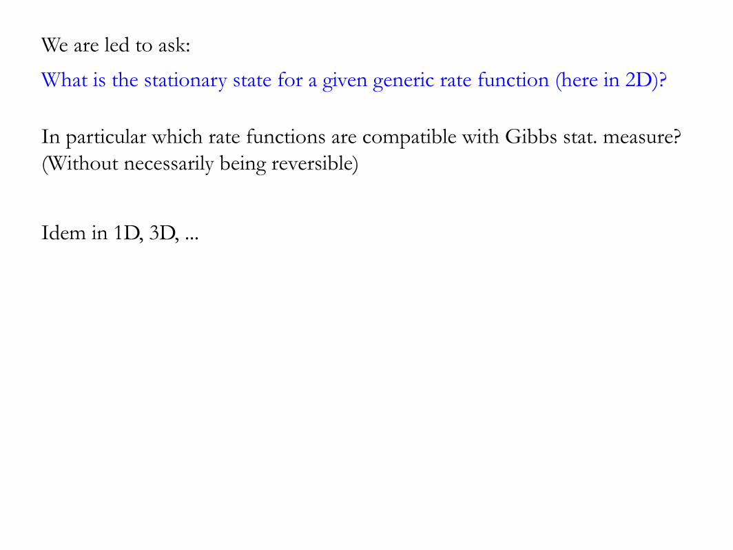
We are led to ask:

What is the stationary state for a given generic rate function (here in 2D)?

In particular which rate functions are compatible with Gibbs stat. measure? (Without necessarily being reversible)

Idem in 1D, 3D, ...

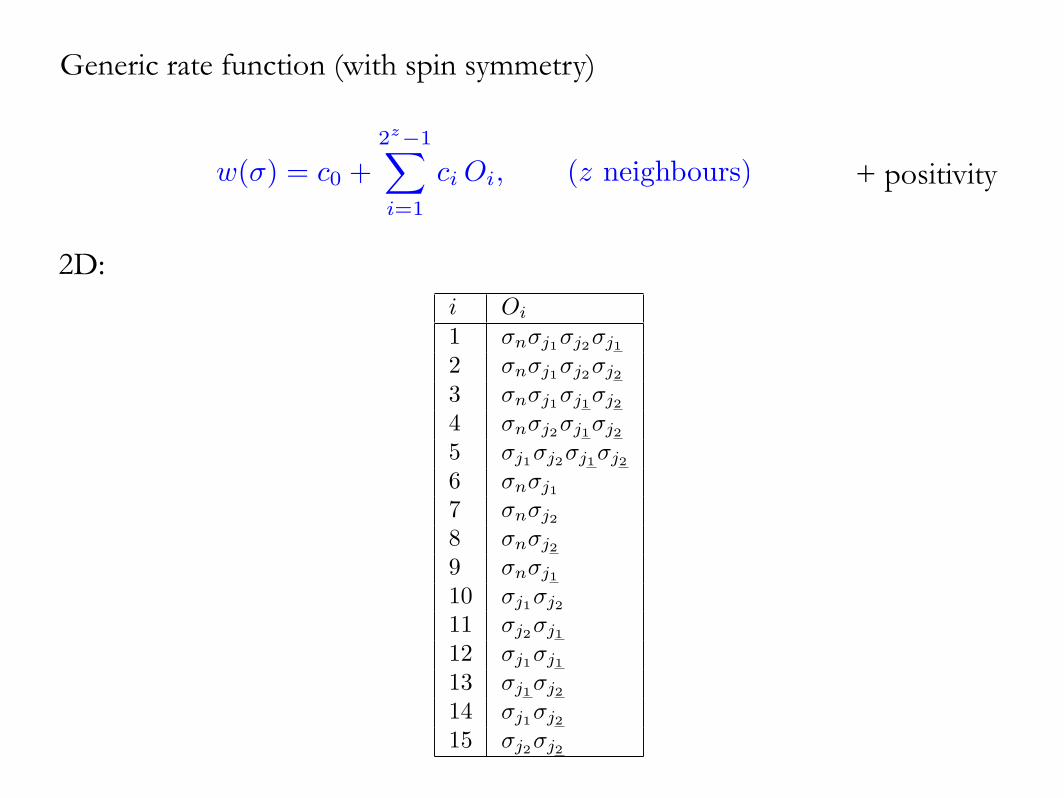
Generic rate function (with spin symmetry)

i Oi

1 σnσj1σj2σj1

2 σnσj1σj2σj2

3 σnσj1σj1σj2

4 σnσj2σj1σj2

5 σj1σj2σj1σj2

6 σnσj1

7 σnσj2

8 σnσj2

9 σnσj1

10 σj1σj2

11 σj2σj1

12 σj1σj1

13 σj1σj2

14 σj1σj2

15 σj2σj2

2D:

+ positivityw(σ) = c0 +2z−1�

i=1

ci Oi, (z neighbours)

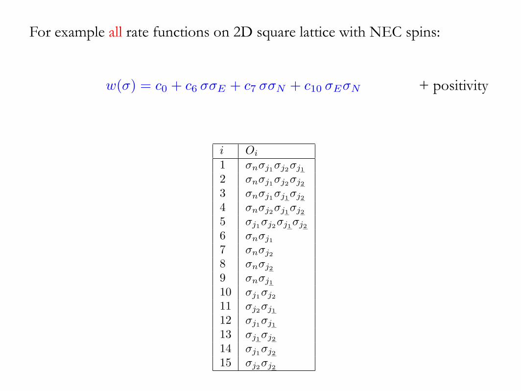
For example all rate functions on 2D square lattice with NEC spins:

i Oi

1 σnσj1σj2σj1

2 σnσj1σj2σj2

3 σnσj1σj1σj2

4 σnσj2σj1σj2

5 σj1σj2σj1σj2

6 σnσj1

7 σnσj2

8 σnσj2

9 σnσj1

10 σj1σj2

11 σj2σj1

12 σj1σj1

13 σj1σj2

14 σj1σj2

15 σj2σj2

+ positivityw(σ) = c0 + c6 σσE + c7 σσN + c10 σEσN

Künsch:

Lima&Stauffer:

γ = tanh 2K (K = J/T )

w(σ) = c0(1− γ σ(σE + σN ) + γ2σEσN )

w(σ) = c0(1− 12γ σ(σE + σN ))

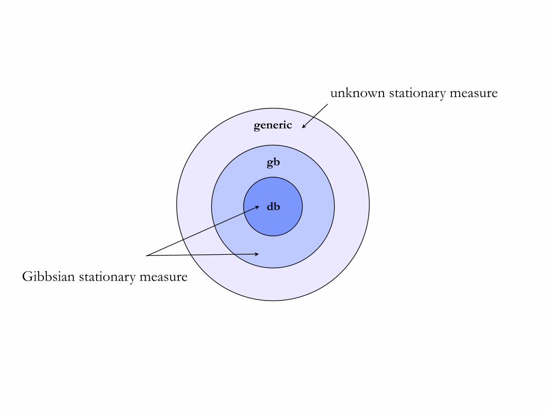
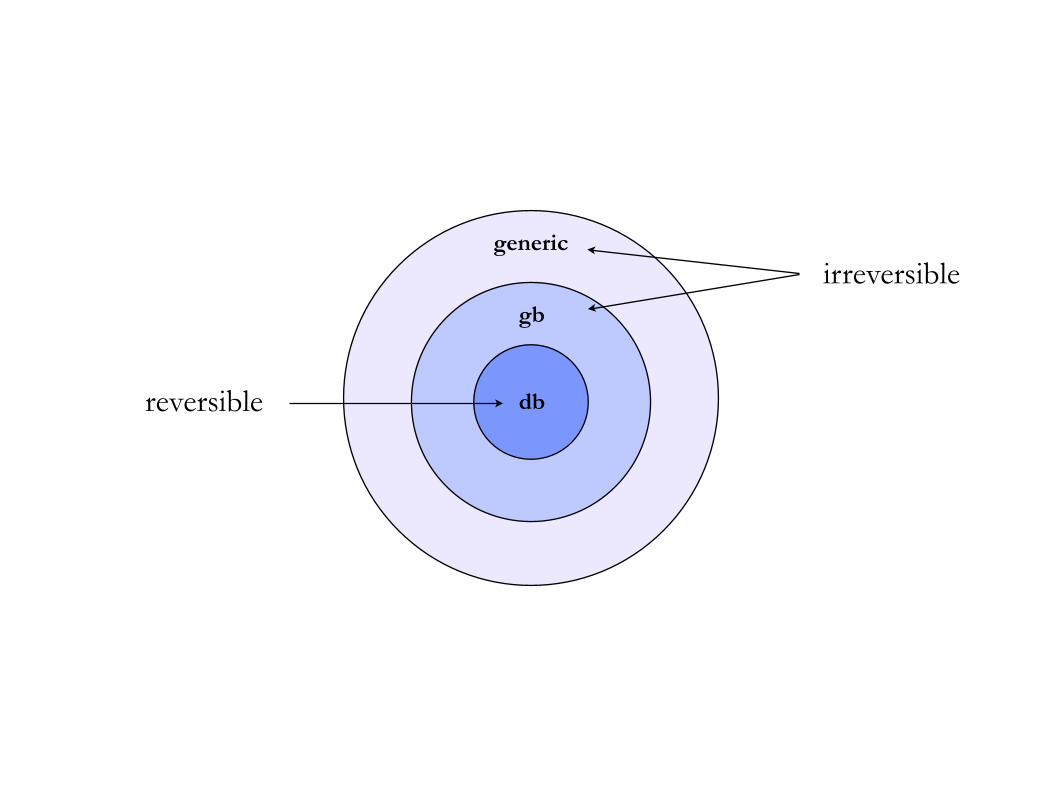
A priori expected classification

(in the space of coefficients defining the rate function):

db

gb

generic

db

gb

generic

unknown stationary measure

Gibbsian stationary measure

db

gb

genericirreversible

reversible

db

gb

generic

db

gb

generic

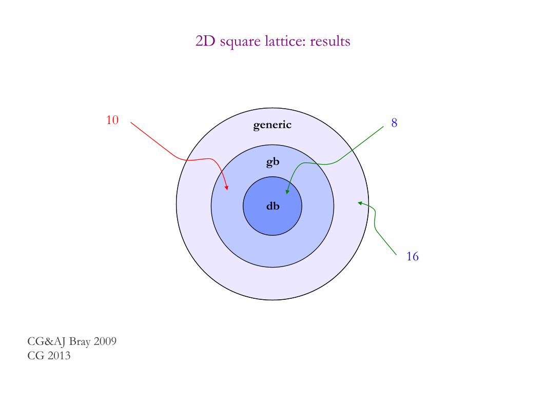
2D square lattice: results

16

810

CG&AJ Bray 2009CG 2013

db

gb

generic

db

gb

generic

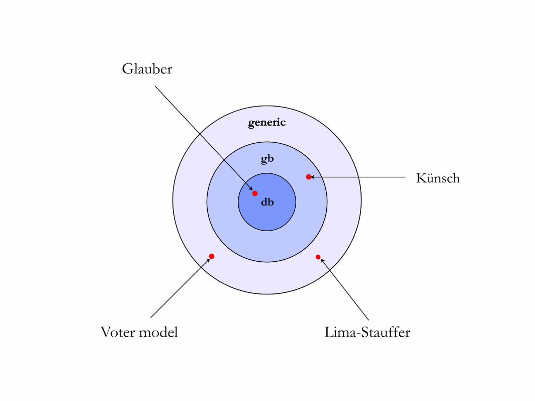
Voter model Lima-Stauffer

Künsch

Glauber

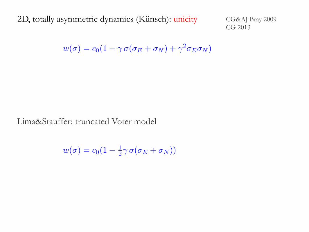
2D, totally asymmetric dynamics (Künsch): unicity

w(σ) = c0(1− γ σ(σE + σN ) + γ2σEσN )

Lima&Stauffer: truncated Voter model

w(σ) = c0(1− 12γ σ(σE + σN ))

CG&AJ Bray 2009CG 2013

generic (16)

symdb gb

reversible (8) Gibbs (10)symmetric (5)

sym symdb gb

reversible symmetric (3)

irreversasym irrevers asym

TA (1)

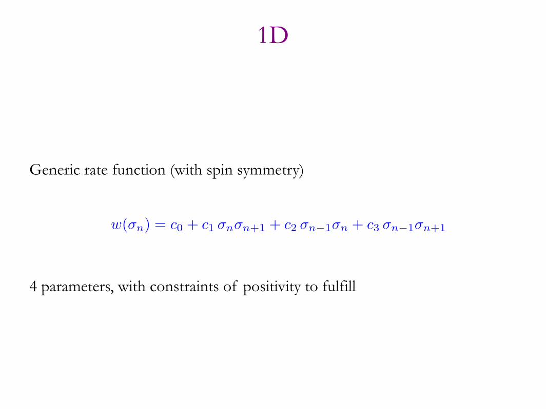
Generic rate function (with spin symmetry)

4 parameters, with constraints of positivity to fulfill

w(σn) = c0 + c1 σnσn+1 + c2 σn−1σn + c3 σn−1σn+1

1D

db

gb

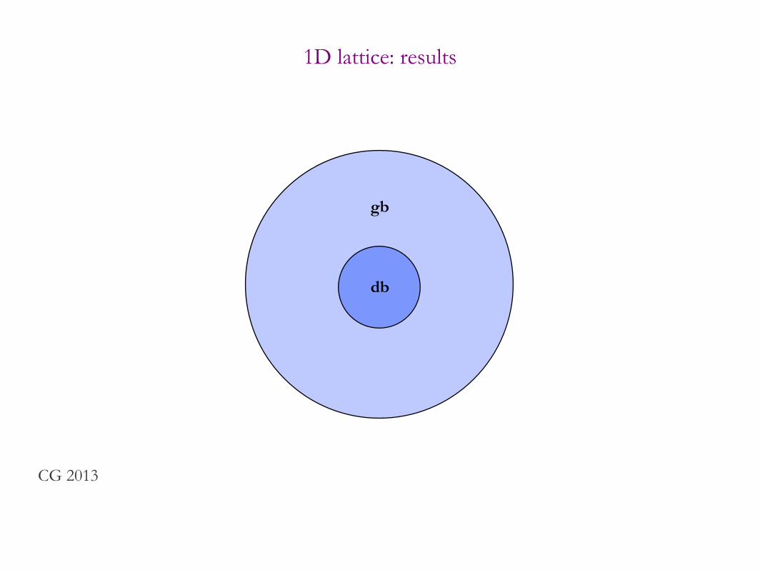
1D lattice: results

CG 2013

db

gb

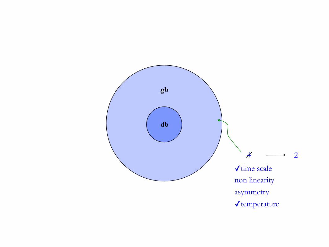
1D lattice: results

2

4

db

gb

✓time scalenon linearityasymmetry

✓temperature

4 2

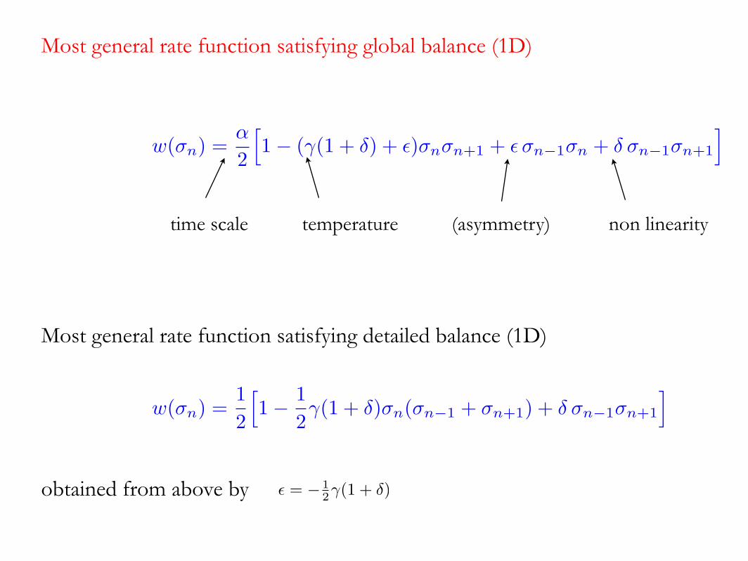
Most general rate function satisfying global balance (1D)

non linearity(asymmetry)time scale temperature

Most general rate function satisfying detailed balance (1D)

obtained from above by

w(σn) =α

2

�1− (γ(1 + δ) + �)σnσn+1 + � σn−1σn + δ σn−1σn+1

�

w(σn) =12

�1− 1

2γ(1 + δ)σn(σn−1 + σn+1) + δ σn−1σn+1

�

� = − 12γ(1 + δ)

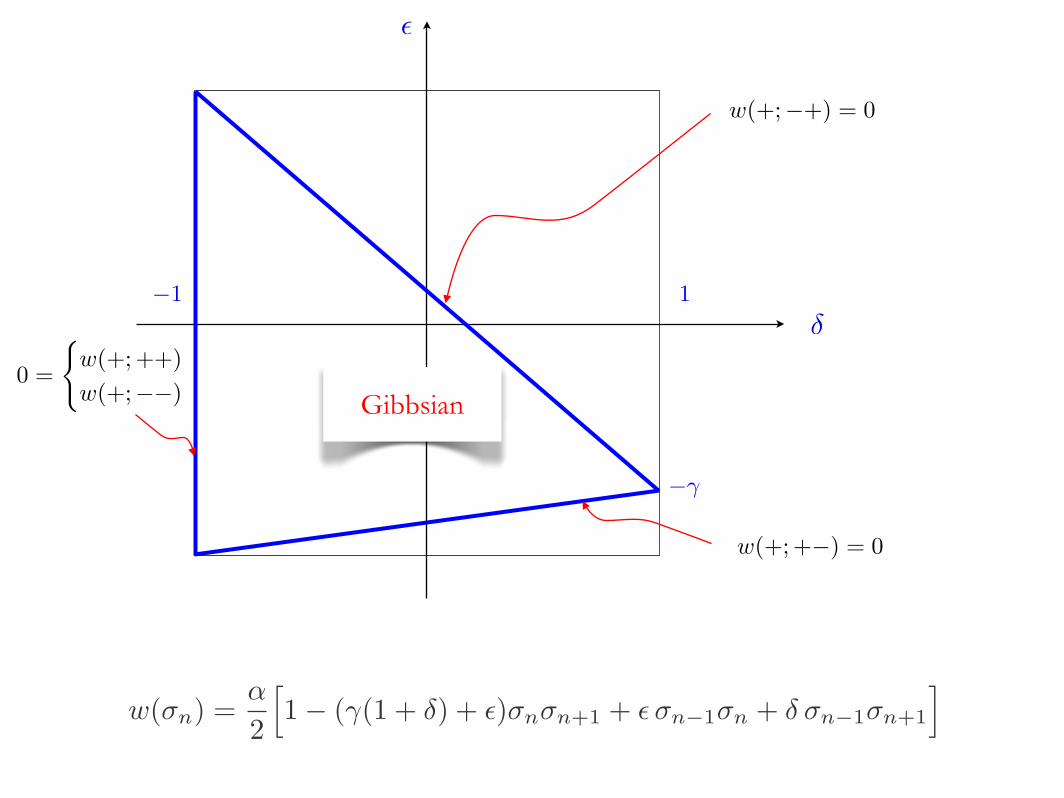
−1 1

−γ

�

δ

w(+; +−) = 0

w(+;−+) = 0

0 =

�w(+; ++)w(+;−−)

w(σn) =α

2

�1− (γ(1 + δ) + �)σnσn+1 + � σn−1σn + δ σn−1σn+1

�

Gibbsian

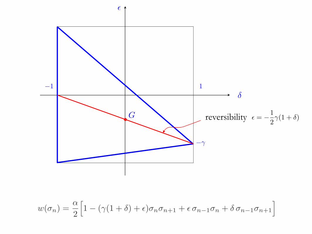
−1 1

−γ

reversibility

�

δ

� = −12γ(1 + δ)G

w(σn) =α

2

�1− (γ(1 + δ) + �)σnσn+1 + � σn−1σn + δ σn−1σn+1

�

−1 1

−γ

�

δ

G

δ = 0integrability

w(σn) =α

2

�1− (γ(1 + δ) + �)σnσn+1 + � σn−1σn + δ σn−1σn+1

�

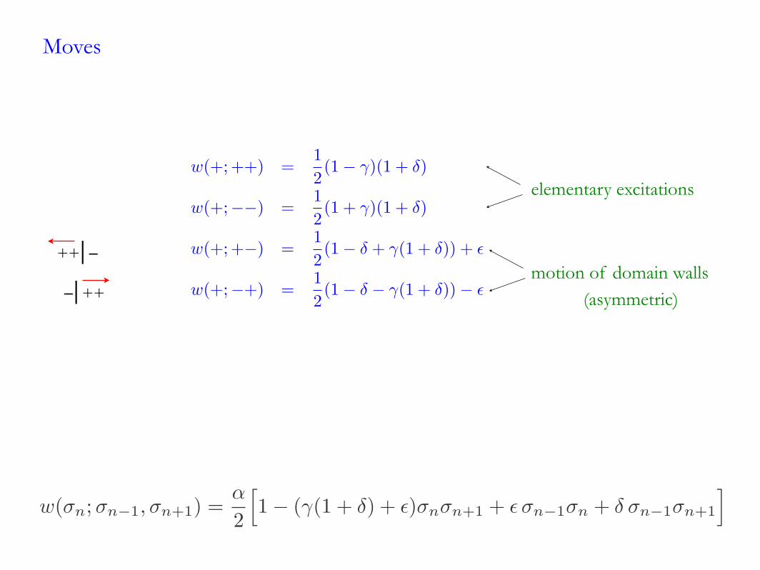
elementary excitations

motion of domain walls

w(+; ++) =12(1− γ)(1 + δ)

w(+;−−) =12(1 + γ)(1 + δ)

w(+; +−) =12(1− δ + γ(1 + δ)) + �

w(+;−+) =12(1− δ − γ(1 + δ))− �

++⎢−

−⎢++

Moves

(asymmetric)

w(σn;σn−1, σn+1) =α

2

�1− (γ(1 + δ) + �)σnσn+1 + � σn−1σn + δ σn−1σn+1

�

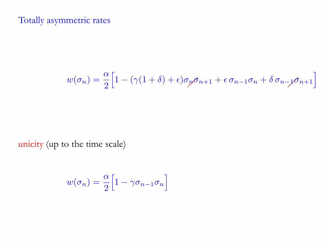
Totally asymmetric rates

unicity (up to the time scale)

w(σn) =α

2

�1− (γ(1 + δ) + �)σnσn+1 + � σn−1σn + δ σn−1σn+1

�

w(σn) =α

2

�1− γσn−1σn

�

−1 1

−γ

�

δ

G

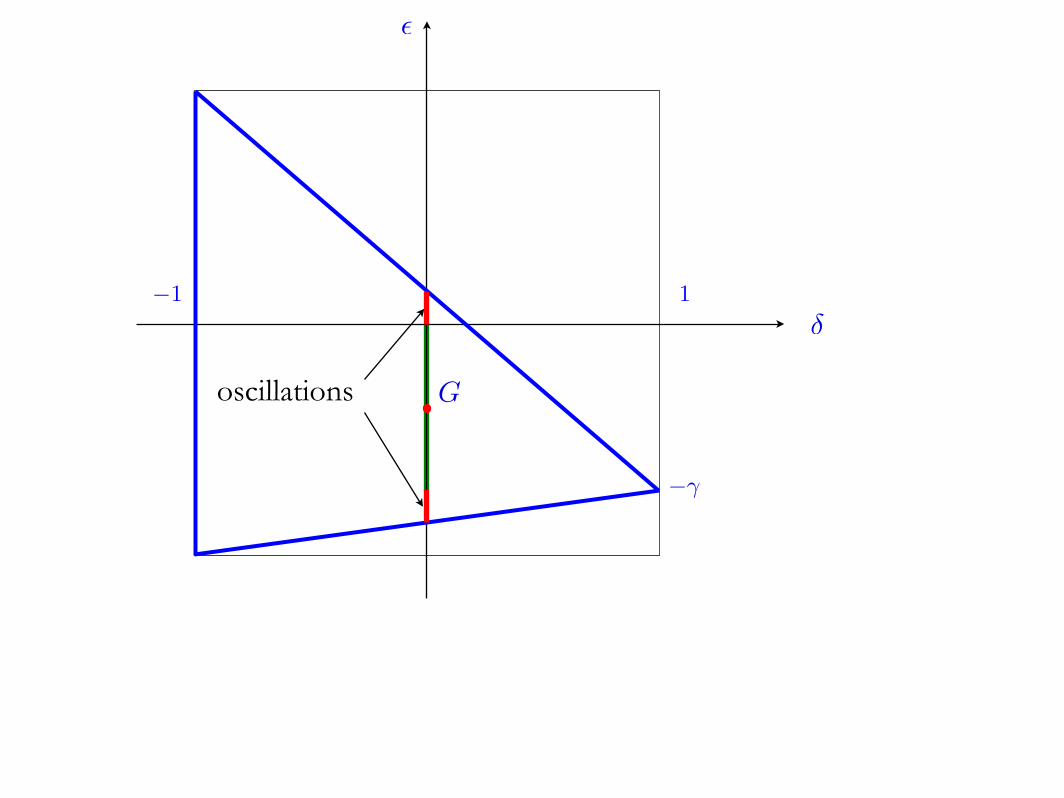
totally asymmetric

w =12

�1− γσn−1σn

�, w =

12

�1− γσnσn+1

�

−1 1

−γ

�

δ

Goscillations

−1 1

−γ

�

δ

G

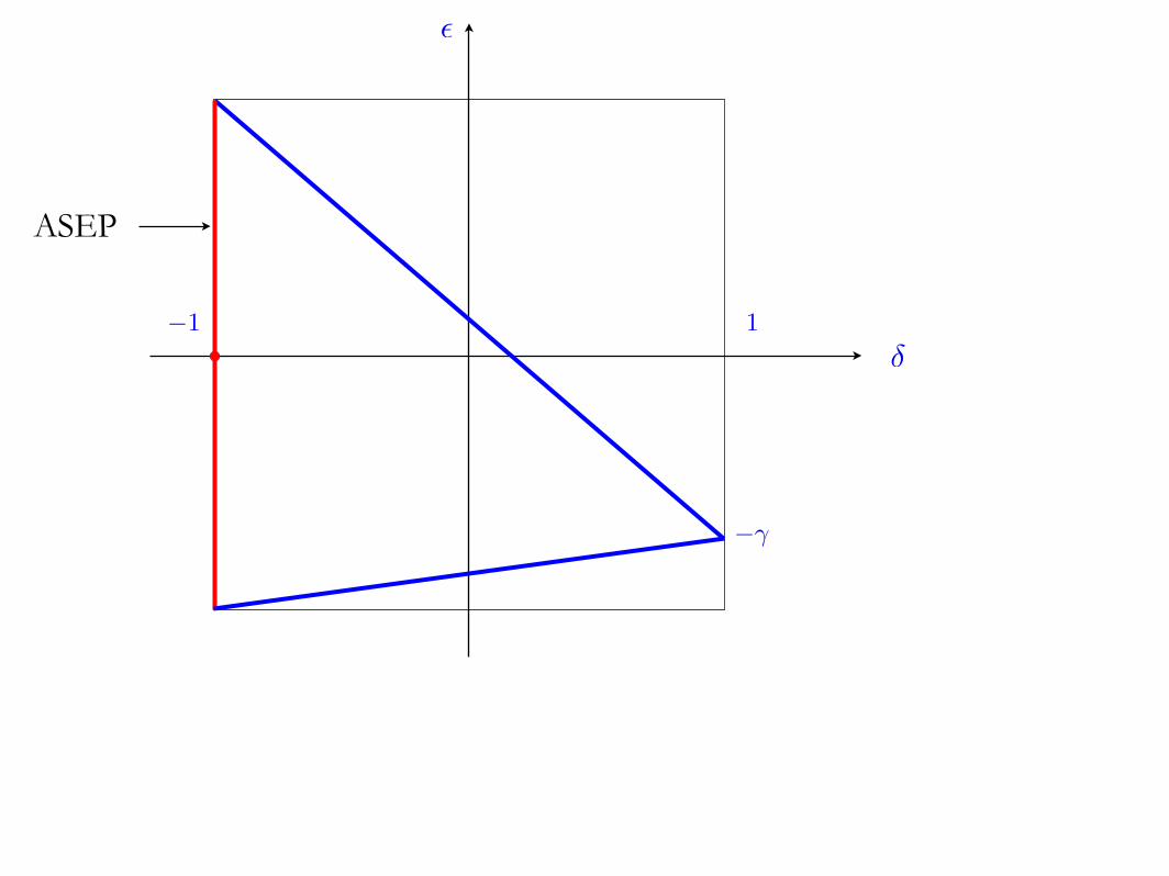
SEPreversible

−1 1

−γ

�

δ

ASEP

−1 1

−γ

�

δ

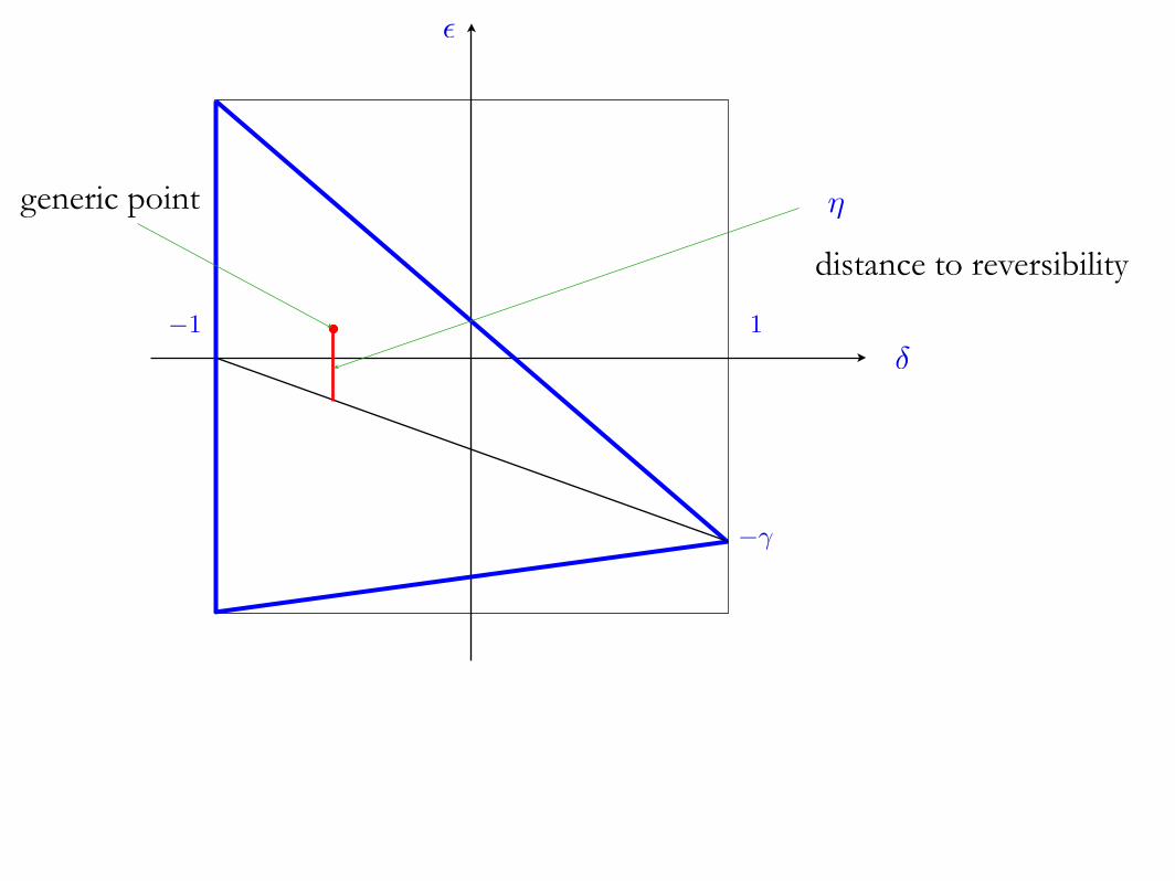
generic point

distance to reversibility

η

In 1D

In 2D, for those special rates leading to Gibbsian stat. state

What can be said on the fluctuations of the system in the stat. state?

What can be said on the transient?

What can be said on the stationary state?

Observables (1D)

relaxation of system to stationary state

fluctuations of system in stationary state

Cstat(t) = �σ0(0)σ0(t)� (thermalized initial state)

Ctransient(t) = �σ0(0)σ0(t)� (disordered initial state)

Glauber

α = 1− γ

cf. fluctuation-dissipation theorem at equilibrium

Ctransient(t) = e−tI0(γt) ∼ e−αt

Cstat(t) =�

1− γ2

� ∞

tdu Ctransient(u) ∼ e−αt

Glauber 1963

−1 1

−γ

�

δ

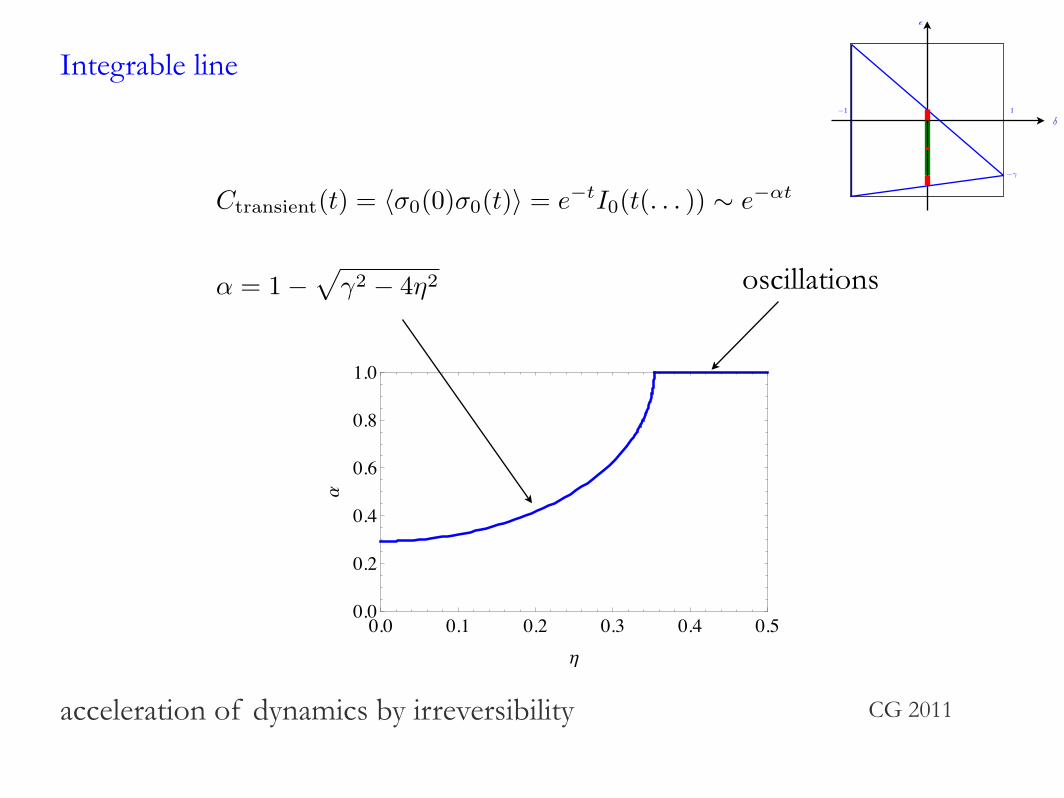
Integrable line

Ctransient(t) = �σ0(0)σ0(t)� = e−tI0(t(. . . )) ∼ e−αt

α = 1−�

γ2 − 4η2

acceleration of dynamics by irreversibility

oscillations

−1 1

−γ

�

δ

CG 2011

0.0 0.1 0.2 0.3 0.4 0.50.0

0.2

0.4

0.6

0.8

1.0

Η

Α

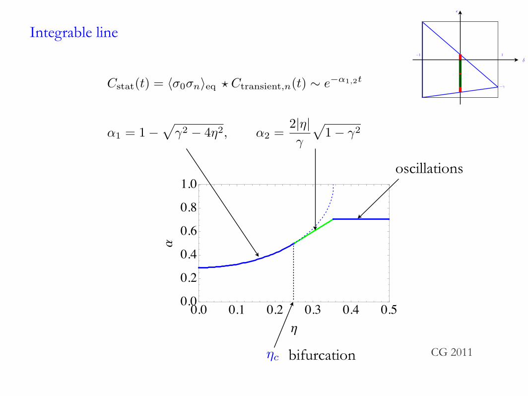
Integrable line

oscillations

α1 = 1−�

γ2 − 4η2, α2 =2|η|γ

�1− γ2

bifurcation

Cstat(t) = �σ0σn�eq � Ctransient,n(t) ∼ e−α1,2t

CG 2011

0.0 0.1 0.2 0.3 0.4 0.50.0

0.2

0.4

0.6

0.8

1.0

Η

Α

ηc

−1 1

−γ

�

δ

!

!"#

!"#

$

$$

$$

%&'

%&'

($

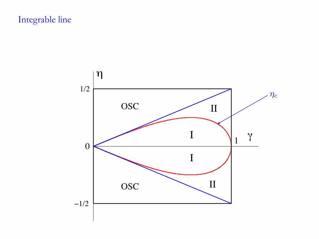
Integrable line

ηc

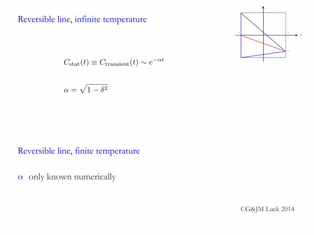
Reversible line, infinite temperature

Cstat(t) ≡ Ctransient(t) ∼ e−αt

α =�

1− δ2

Reversible line, finite temperature

only known numerically

CG&JM Luck 2014

α

−1 1

−γ

�

δ

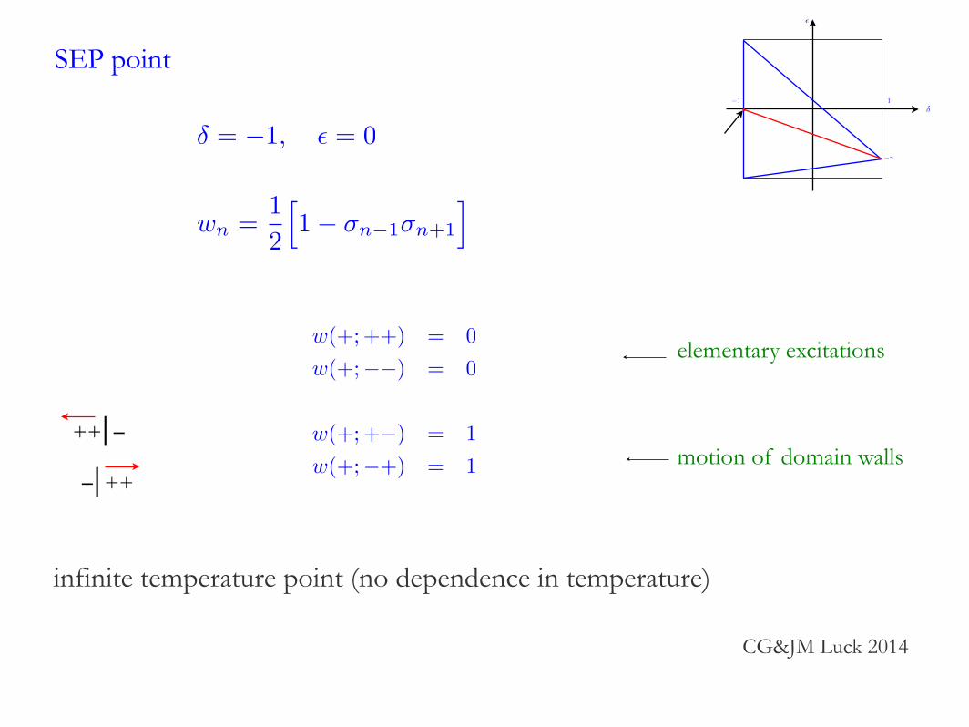
δ = −1, � = 0

elementary excitations

motion of domain walls++⎢−

−⎢++

w(+; ++) = 0w(+;−−) = 0

w(+; +−) = 1w(+;−+) = 1

SEP point

wn =12

�1− σn−1σn+1

�

infinite temperature point (no dependence in temperature)

−1 1

−γ

�

δ

CG&JM Luck 2014

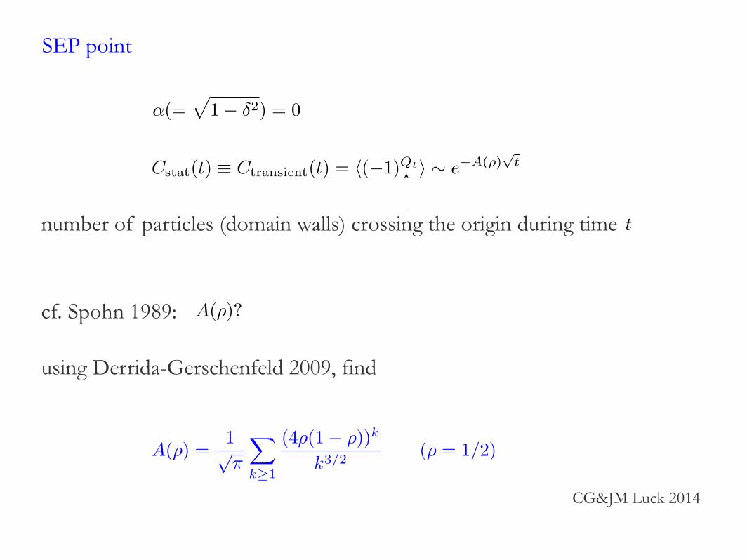
SEP point

α(=�

1− δ2) = 0

cf. Spohn 1989: A(ρ)?

using Derrida-Gerschenfeld 2009, find

A(ρ) =1√π

�

k≥1

(4ρ(1− ρ))k

k3/2(ρ = 1/2)

Cstat(t) ≡ Ctransient(t) = �(−1)Qt� ∼ e−A(ρ)√

t

number of particles (domain walls) crossing the origin during time t

CG&JM Luck 2014

elementary excitations

motion of domain walls++⎢−

−⎢++

δ = −1

w(+; ++) = 0w(+;−−) = 0

w(+; +−) = 1 + �

w(+;−+) = 1− �

ASEP line

wn =12

�1 + � σn(σn−1 − σn+1)− σn−1σn+1

�

Cstat(t) ≡ Ctransient(t) ∼ e−B(ρ)√

t, B(ρ)?

conjecture:

use Tracy-Widom 2010

−1 1

−γ

�

δ

CG&JM Luck 2014

2D

2D paramagnetic phase shares a number of properties of 1D

2D ferromagnetic phase, qualitatively different from 1D: ballistic coarsening,

power law persistence (while exponential in 1D), metastable/blocked configurations

CG&M Pleimling 2014

db

gb

generic

db

generic

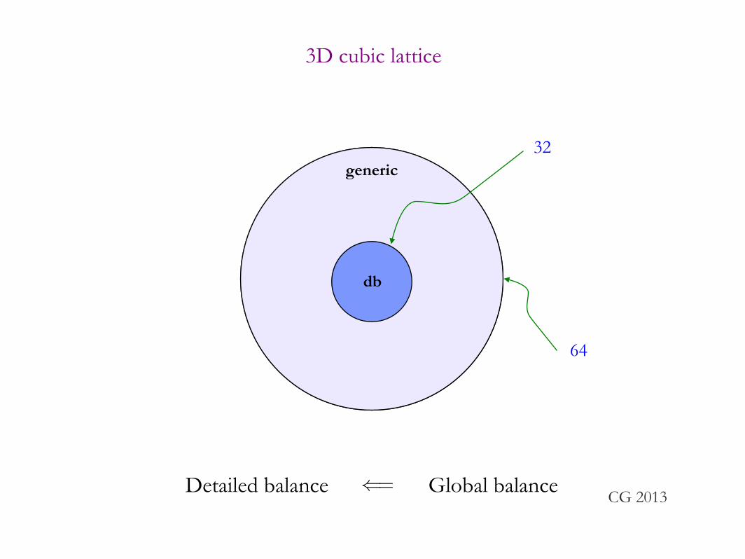
3D cubic lattice

64

32

Detailed balance Global balance⇐=CG 2013

More

- Relation to 2D Toom model

- Entropy production

- ...