dynamics of a particle in some cases of the n-body problem · dynamics of a particle in some cases...
TRANSCRIPT
Dynamics of a particle in some cases of theN -body problem
Elipe, A.(1,2)
1Grupo de Mecánica Espacial. (IUMA)2Centro Universitario de la Defensa. Zaragoza
A.Elipe (GME, UZ) D-Days 2016. Salou November 2016 1 / 25
Introduction
Motivation
Two-body problem (no secrets)N -body problem (too difficult)R3BP (still difficult and 200 years of history)Add complications to the R3BP (non spherity, radiation pressure. . . , ribbon,. . . )Crazy models, but accepted in “journals”
A.Elipe (GME, UZ) D-Days 2016. Salou November 2016 2 / 25

Introduction
Motivation
thousands of exoplanets discoveredextrasolar systems with one or several stars and none or severalplanetsmotion of small particles (dust)⇒ force of radiationforce can be very big compared with the gravity force (Lamy &Perrin, 1997)This problem is a generalization of the classical RTBwith radiation emitted from the primaries (Schuerman, 1980).A rich dynamics
A.Elipe (GME, UZ) D-Days 2016. Salou November 2016 3 / 25

Formulation of the problem
• we consider the Restricted collinear four-body problem with radiationpressure
• 3 primaries:(P0,m0, q0) and two identical bodies (P1,m, q), (P2,m, q)
• planar motion of a massless P in a synodic reference frame
m0 = βm, ω2 = ∆ = 2(1 + 4β)
A.Elipe (GME, UZ) D-Days 2016. Salou November 2016 4 / 25

Formulation of the problem
Radiation coefficients
b =FrFg→ qi = 1− bi
bi = 0 classical problembi ∈ (0, 1) reduction of gravitational forces by radiationbi ≥ 1 radiation has overhelmed gravitational forces by radiation
So, qi ∈ (−∞, 1] (i = 0, 1, 2)
A.Elipe (GME, UZ) D-Days 2016. Salou November 2016 5 / 25
Formulation of the problem
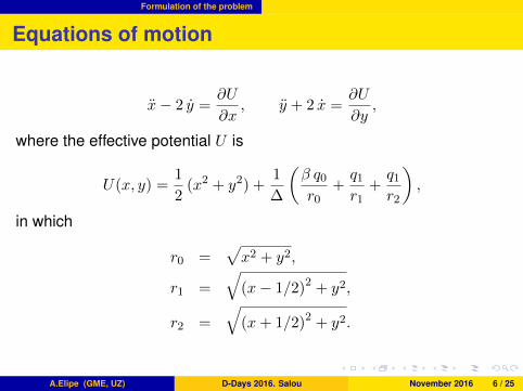
Equations of motion
x− 2 y =∂U
∂x, y + 2 x =
∂U
∂y,
where the effective potential U is
U(x, y) =1
2(x2 + y2) +
1
∆
(β q0r0
+q1r1
+q1r2
),
in which
r0 =√x2 + y2,
r1 =
√(x− 1/2)2 + y2,
r2 =
√(x+ 1/2)2 + y2.
A.Elipe (GME, UZ) D-Days 2016. Salou November 2016 6 / 25

Equilibrium points
Equilibrium points
Ux = x− 1
∆
[β q0r30
x+q1r31
(x− 1
2
)+q1r32
(x+ 1
2
)]= 0,
Uy = y
[1− 1
∆
(β q0r30
+q1r31
+q1r32
)]= 0.
Two types of solutions:
• triangular points when y 6= 0• collinear points when y = 0
A.Elipe (GME, UZ) D-Days 2016. Salou November 2016 7 / 25
Equilibrium points Triangular points (y 6= 0)
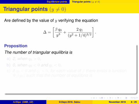
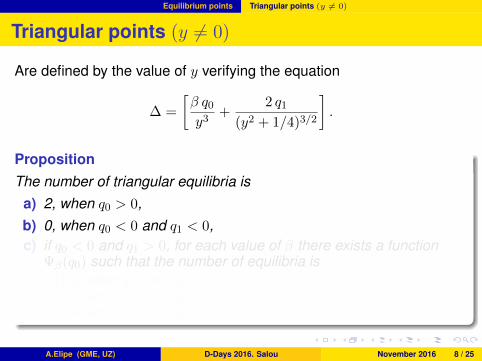
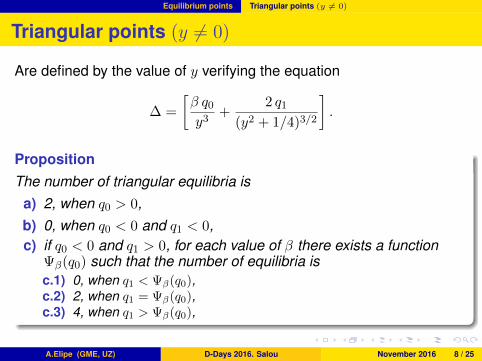
Triangular points (y 6= 0)
Are defined by the value of y verifying the equation
∆ =
[β q0y3
+2 q1
(y2 + 1/4)3/2
].
PropositionThe number of triangular equilibria is
a) 2, when q0 > 0,b) 0, when q0 < 0 and q1 < 0,c) if q0 < 0 and q1 > 0, for each value of β there exists a function
Ψβ(q0) such that the number of equilibria isc.1) 0, when q1 < Ψβ(q0),c.2) 2, when q1 = Ψβ(q0),c.3) 4, when q1 > Ψβ(q0),
A.Elipe (GME, UZ) D-Days 2016. Salou November 2016 8 / 25

Equilibrium points Triangular points (y 6= 0)
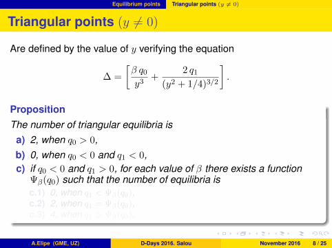
Triangular points (y 6= 0)
Are defined by the value of y verifying the equation
∆ =
[β q0y3
+2 q1
(y2 + 1/4)3/2
].
PropositionThe number of triangular equilibria is
a) 2, when q0 > 0,b) 0, when q0 < 0 and q1 < 0,c) if q0 < 0 and q1 > 0, for each value of β there exists a function
Ψβ(q0) such that the number of equilibria isc.1) 0, when q1 < Ψβ(q0),c.2) 2, when q1 = Ψβ(q0),c.3) 4, when q1 > Ψβ(q0),
A.Elipe (GME, UZ) D-Days 2016. Salou November 2016 8 / 25
Equilibrium points Triangular points (y 6= 0)
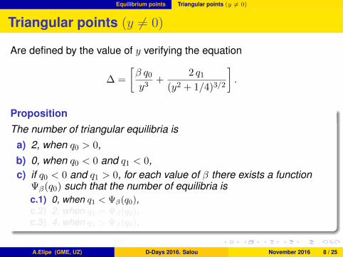
Triangular points (y 6= 0)
Are defined by the value of y verifying the equation
∆ =
[β q0y3
+2 q1
(y2 + 1/4)3/2
].
PropositionThe number of triangular equilibria is
a) 2, when q0 > 0,b) 0, when q0 < 0 and q1 < 0,c) if q0 < 0 and q1 > 0, for each value of β there exists a function
Ψβ(q0) such that the number of equilibria isc.1) 0, when q1 < Ψβ(q0),c.2) 2, when q1 = Ψβ(q0),c.3) 4, when q1 > Ψβ(q0),
A.Elipe (GME, UZ) D-Days 2016. Salou November 2016 8 / 25
Equilibrium points Triangular points (y 6= 0)
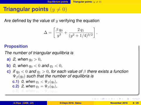
Triangular points (y 6= 0)
Are defined by the value of y verifying the equation
∆ =
[β q0y3
+2 q1
(y2 + 1/4)3/2
].
PropositionThe number of triangular equilibria is
a) 2, when q0 > 0,b) 0, when q0 < 0 and q1 < 0,c) if q0 < 0 and q1 > 0, for each value of β there exists a function
Ψβ(q0) such that the number of equilibria isc.1) 0, when q1 < Ψβ(q0),c.2) 2, when q1 = Ψβ(q0),c.3) 4, when q1 > Ψβ(q0),
A.Elipe (GME, UZ) D-Days 2016. Salou November 2016 8 / 25
Equilibrium points Triangular points (y 6= 0)
Triangular points (y 6= 0)
Are defined by the value of y verifying the equation
∆ =
[β q0y3
+2 q1
(y2 + 1/4)3/2
].
PropositionThe number of triangular equilibria is
a) 2, when q0 > 0,b) 0, when q0 < 0 and q1 < 0,c) if q0 < 0 and q1 > 0, for each value of β there exists a function
Ψβ(q0) such that the number of equilibria isc.1) 0, when q1 < Ψβ(q0),c.2) 2, when q1 = Ψβ(q0),c.3) 4, when q1 > Ψβ(q0),
A.Elipe (GME, UZ) D-Days 2016. Salou November 2016 8 / 25
Equilibrium points Collinear points (y = 0)
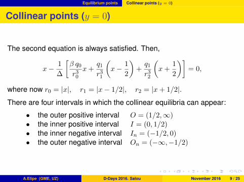
Collinear points (y = 0)
The second equation is always satisfied. Then,
x− 1
∆
[β q0r30
x+q1r31
(x− 1
2
)+q1r32
(x+
1
2
)]= 0,
where now r0 = |x|, r1 = |x− 1/2|, r2 = |x+ 1/2|.
There are four intervals in which the collinear equilibria can appear:
• the outer positive interval O = (1/2,∞)• the inner positive interval I = (0, 1/2)• the inner negative interval In = (−1/2, 0)• the outer negative interval On = (−∞,−1/2)
A.Elipe (GME, UZ) D-Days 2016. Salou November 2016 9 / 25
Equilibrium points Collinear points (y = 0)
Outer collinear equilibria
PropositionThe number of positive outer collinear equilibria, regardless of thevalue of β, is
a) 0, when q1 < 0,b) 1, when q1 > 0.
A.Elipe (GME, UZ) D-Days 2016. Salou November 2016 10 / 25

Equilibrium points Collinear points (y = 0)
Outer collinear equilibria
PropositionThe number of positive outer collinear equilibria, regardless of thevalue of β, is
a) 0, when q1 < 0,b) 1, when q1 > 0.
A.Elipe (GME, UZ) D-Days 2016. Salou November 2016 10 / 25

Equilibrium points Collinear points (y = 0)
Outer collinear equilibria
PropositionThe number of positive outer collinear equilibria, regardless of thevalue of β, is
a) 0, when q1 < 0,b) 1, when q1 > 0.
A.Elipe (GME, UZ) D-Days 2016. Salou November 2016 10 / 25

Equilibrium points Collinear points (y = 0)
Inner collinear equilibria
PropositionThe number of positive inner collinear equilibria is
a) 1, when q1 > 0 and q0 > 0,b) 0, when q1 > 0 and q0 < 0,c) 1, when q1 < 0 and q0 < 0,d) if q1 < 0 and q0 > 0, for each value of β there exists a function
Φβ(q0) such that the number of equilibria is:d.1) 0, when q1 < Φβ(q0),d.2) 1, when q1 = Φβ(q0),d.3) 2, when q1 > Φβ(q0).
A.Elipe (GME, UZ) D-Days 2016. Salou November 2016 11 / 25

Regions with different number of equilibrium points
Region For any β Equilibria(T ;NO, NI , PI , PO)
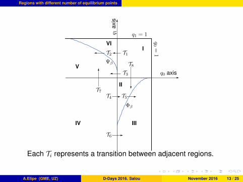
I q0 ∈ [0, 1] q1 ∈ [0, 1] (2; 1,1,1,1)II q0 ∈ [0, 1] q1 ∈ (Φβ(q0), 0) (2; 0,2,2,0)Φβ curve q0 ∈ [0, 1] q1 = Φβ(q0) (2; 0,1,1,0)III q0 ∈ [0, 1] q1 < Φβ(q0) (2; 0,0,0,0)IV q0 < 0 q1 < 0 (0; 0,1,1,0)V q0 < 0 q1 ∈ (0,Ψβ(q0)) (0; 1,0,0,1)Ψβ curve q0 < 0 q1 = Ψβ(q0) (2; 1,0,0,1)VI q0 < 0 q1 > Ψβ(q0) (4; 1,0,0,1)
Six regions and two bifurcation curves
A.Elipe (GME, UZ) D-Days 2016. Salou November 2016 12 / 25
Regions with different number of equilibrium points
IVI
ΨβV
IV
II
Φβ
III
� T1� T2
� T3
-T4 T5 -
-T6
6
T7?
T8
6
q 1ax
is
q1 = 1
-q0 axis
q0
=1
Each Ti represents a transition between adjacent regions.
A.Elipe (GME, UZ) D-Days 2016. Salou November 2016 13 / 25

Regions with different number of equilibrium points
Transitions between adjacent regions (a)
T1 I→ VI T3 I→ V
Region I Region V Region VI
A.Elipe (GME, UZ) D-Days 2016. Salou November 2016 14 / 25
Regions with different number of equilibrium points
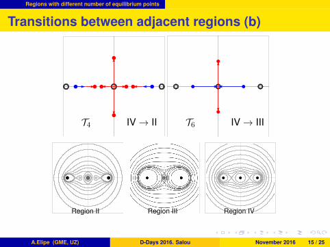
Transitions between adjacent regions (b)
T4 IV→ II T6 IV→ III
Region II Region III Region IV
A.Elipe (GME, UZ) D-Days 2016. Salou November 2016 15 / 25
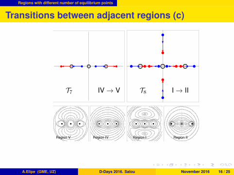
Regions with different number of equilibrium points
Transitions between adjacent regions (c)
T7 IV→ V T8 I→ II
Region V Region IV Region I Region II
A.Elipe (GME, UZ) D-Days 2016. Salou November 2016 16 / 25

Regions with different number of equilibrium points
Transition T2
Transition from region VI to region V.Through a saddle-node bifurcation.
Figure: Transition T2: saddle-node bifurcation of triangular equilibrium oncurve q1 = Ψβ(q0). Left: two equilibria in region VI. Center: one cuspequilibrium in bifurcation line. Right: no equilibrium in region V
A.Elipe (GME, UZ) D-Days 2016. Salou November 2016 17 / 25
Regions with different number of equilibrium points
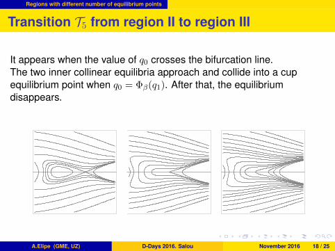
Transition T5 from region II to region III
It appears when the value of q0 crosses the bifurcation line.The two inner collinear equilibria approach and collide into a cupequilibrium point when q0 = Φβ(q1). After that, the equilibriumdisappears.
A.Elipe (GME, UZ) D-Days 2016. Salou November 2016 18 / 25
Regions with different number of equilibrium points
Linear stability of the equilibrium points
It is characterized by the roots of the characteristic equation:
λ4 + a λ2 + b = 0,
where coefficients
a = 4 − Uxx − Uyy, b = Uxx Uyy − U2xy
depend on the three parameters β, q0, q1 and the coordinates,x(β, q0, q1) and y(β, q0, q1), of the equilibrium points
A.Elipe (GME, UZ) D-Days 2016. Salou November 2016 19 / 25
Regions with different number of equilibrium points Stability of triangular equilibria
Stability of triangular equilibria
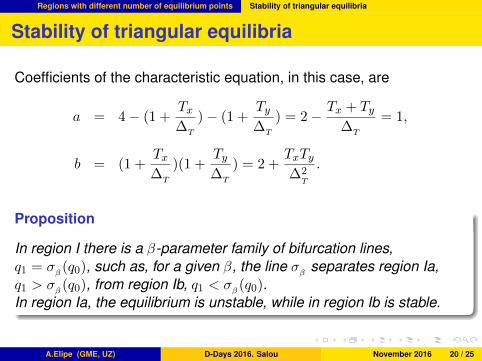
Coefficients of the characteristic equation, in this case, are
a = 4− (1 +Tx∆T
)− (1 +Ty∆T
) = 2− Tx + Ty∆T
= 1,
b = (1 +Tx∆T
)(1 +Ty∆T
) = 2 +TxTy∆2T
.
Proposition
In region I there is a β-parameter family of bifurcation lines,q1 = σ
β(q0), such as, for a given β, the line σ
βseparates region Ia,
q1 > σβ(q0), from region Ib, q1 < σ
β(q0).
In region Ia, the equilibrium is unstable, while in region Ib is stable.
A.Elipe (GME, UZ) D-Days 2016. Salou November 2016 20 / 25
Regions with different number of equilibrium points Stability of triangular equilibria
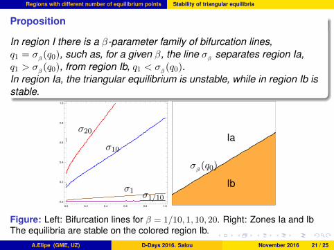
Proposition
In region I there is a β-parameter family of bifurcation lines,q1 = σ
β(q0), such as, for a given β, the line σ
βseparates region Ia,
q1 > σβ(q0), from region Ib, q1 < σ
β(q0).
In region Ia, the triangular equilibrium is unstable, while in region Ib isstable.
σβ(q0)
Ia
Ib
σ20
σ10
σ1 σ1/10
Figure: Left: Bifurcation lines for β = 1/10, 1, 10, 20. Right: Zones Ia and IbThe equilibria are stable on the colored region Ib.
A.Elipe (GME, UZ) D-Days 2016. Salou November 2016 21 / 25
Regions with different number of equilibrium points Stability of triangular equilibria
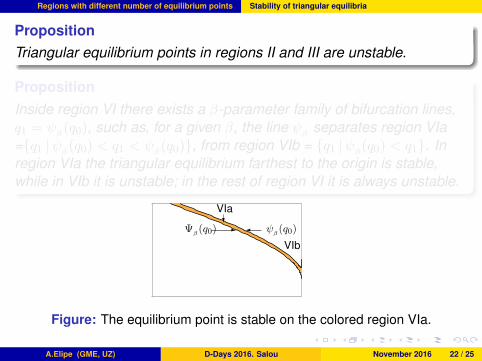
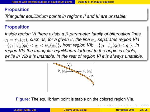
PropositionTriangular equilibrium points in regions II and III are unstable.
PropositionInside region VI there exists a β-parameter family of bifurcation lines,q1 = ψ
β(q0), such as, for a given β, the line ψ
βseparates region VIa
={q1 |ψβ (q0) < q1 < ψβ(q0)}, from region VIb = {q1 |ψβ (q0) < q1}. In
region VIa the triangular equilibrium farthest to the origin is stable,while in VIb it is unstable; in the rest of region VI it is always unstable.
VIb
VIa
ψβ(q0)Ψ
β(q0) - �
?
Figure: The equilibrium point is stable on the colored region VIa.
A.Elipe (GME, UZ) D-Days 2016. Salou November 2016 22 / 25
Regions with different number of equilibrium points Stability of triangular equilibria
PropositionTriangular equilibrium points in regions II and III are unstable.
PropositionInside region VI there exists a β-parameter family of bifurcation lines,q1 = ψ
β(q0), such as, for a given β, the line ψ
βseparates region VIa
={q1 |ψβ (q0) < q1 < ψβ(q0)}, from region VIb = {q1 |ψβ (q0) < q1}. In
region VIa the triangular equilibrium farthest to the origin is stable,while in VIb it is unstable; in the rest of region VI it is always unstable.
VIb
VIa
ψβ(q0)Ψ
β(q0) - �
?
Figure: The equilibrium point is stable on the colored region VIa.
A.Elipe (GME, UZ) D-Days 2016. Salou November 2016 22 / 25
Regions with different number of equilibrium points Stability of collinear equilibria
Stability of collinear equilibria (a)
Two kind of positive collinear equilibria: the outer equilibria, inO = (1/2,∞), and the inner ones, in I = (0, 1/2).
PropositionOuter collinear equilibria in regions I, V and VI are unstable.
PropositionInner collinear equilibria in regions I and IV are unstable.
A.Elipe (GME, UZ) D-Days 2016. Salou November 2016 23 / 25
Regions with different number of equilibrium points Stability of collinear equilibria
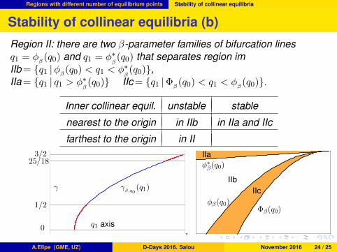
Stability of collinear equilibria (b)
Region II: there are two β-parameter families of bifurcation linesq1 = φ
β(q0) and q1 = φ∗
β(q0) that separates region im
IIb = {q1 |φβ (q0) < q1 < φ∗β(q0)},
IIa = {q1 | q1 > φ∗β(q0)} IIc = {q1 |Φβ
(q0) < q1 < φβ(q0)}.
Inner collinear equil. unstable stable
nearest to the origin in IIb in IIa and IIc
farthest to the origin in II
,
γβ,q0
(q1)
q1 axis
γ
3/225/18
1/2
0
φ∗β(q0)
IIa
IIbIIc
φβ(q0)Φβ(q0)
Figure: Top: γ curve for a pair of values β, qo. Red part represents the valuesof q1 where the equilibrium is stable. Bottom: zones with different stability forthe inner collinear equilibria nearest to the origin. Colored regions IIa, IIcrepresent stable equilibria.
A.Elipe (GME, UZ) D-Days 2016. Salou November 2016 24 / 25

Another problem
Periodic solutions and their parametric evolution in
the planar case of the (n + 1) ring problem with
oblateness
A. Elipe et al. D-Days. Salou. Noviembre 2016. 2
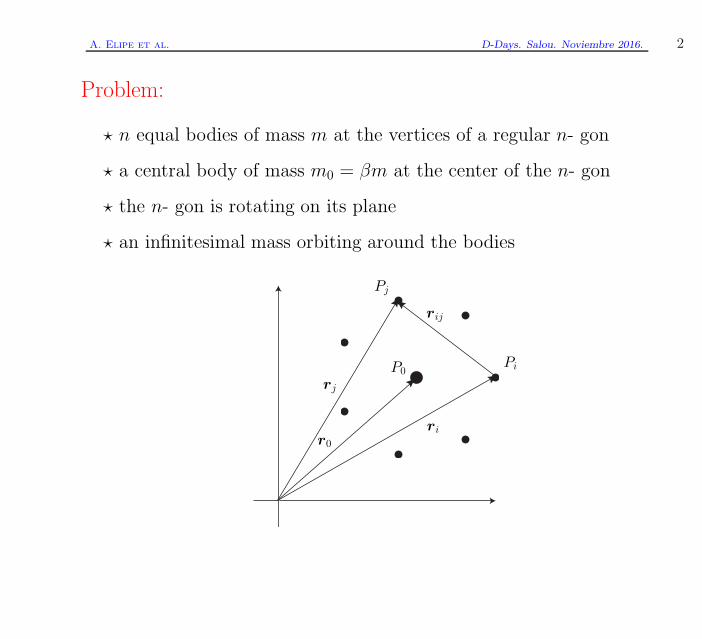
Problem:
⋆ n equal bodies of mass m at the vertices of a regular n- gon
⋆ a central body of mass m0 = βm at the center of the n- gon
⋆ the n- gon is rotating on its plane
⋆ an infinitesimal mass orbiting around the bodies
P0Pi
Pj
rij
rj
ri
r0

A. Elipe et al. D-Days. Salou. Noviembre 2016. 3
An old problem (Maxwell, 1859), Saturn ring
Recent interest:
Astrodynamics, Dynamical systems, . . .
– Scheeres (1992)
– Kalvouridis (1999, 2000, . . . )
– Arribas and Elipe (2004, 2005)
– Pinotsis (2005)
– – –
A. Elipe et al. D-Days. Salou. Noviembre 2016. 4
New problem:
Consider the central body spheroid or radiating source
Consequences:
⋆ A new parameter ǫ
⋆ New equilibria
⋆ New bifurcations
⋆ Dynamics much richer
A. Elipe et al. D-Days. Salou. Noviembre 2016. 5
Equations of motion
x− 2y = −∂U
∂x, y + 2x = −
∂U
∂y,
effective potential
U(x, y) = −1
2(x2 + y2)−
1
∆
(
β
(
1
r0+
ǫ
r20
)
+
n∑
i=1
1
ri
)
,
Introduce the angle θ = π/n, then
xi =1
Mcos 2(i− 1)θ, yi =
1
Msin 2(i− 1)θ,
with M = 2 sin θ, and ∆ = M(Λ + βM2) a constant
Λ = sin2 θn∑
i=2
1
sin(i− 1)θ.
The parameter ǫ ⋚ 0,
Jacobian first integral C = 2U + (x2 + y2)

A. Elipe et al. D-Days. Salou. Noviembre 2016. 6
-2-1
01
2
-2-1
012
-5
-4.5
-4
-3.5
-3
-2-1
01
2
-2-1
012
-2-1
01
2
-2-1
012
-5
-4.5
-4
-3.5
-3
-2-1
01
2
-2-1
012
A. Elipe et al. D-Days. Salou. Noviembre 2016. 7
-2 -1 1 2
-4.5
-3.5
-3
-2 -1 1 2
-5
-4
-3
-2
-1
-2 -1 1 2
-20
-10
10
20
30
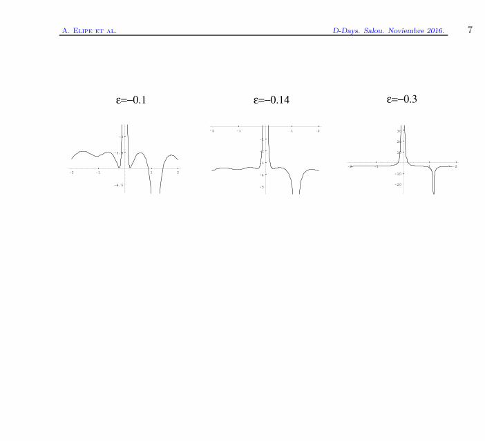
ε=−0.1 ε=−0.14 ε=−0.3
A. Elipe et al. D-Days. Salou. Noviembre 2016. 8
Periodic orbits
β = 2, n = 7, ǫ = −0.1,−0.14 and −0.3;
Grid search in the plane C—x0
Periodic orbits with x- symmetry, then, y0 = 0, x0 = 0
C = (x2
0+ y2
0) + 2U(x0, y0) =⇒ C, x0, y0 = 0, x0 = 0, y0
Integrate until the orbit crosses the x- axis (T/2);
Keep the value x(T/2)
Repeat for x′
0 = x0 + δx0
Check the sign x(T/2)x′(T/2) until negative
Repeat the procedure for another C + δC
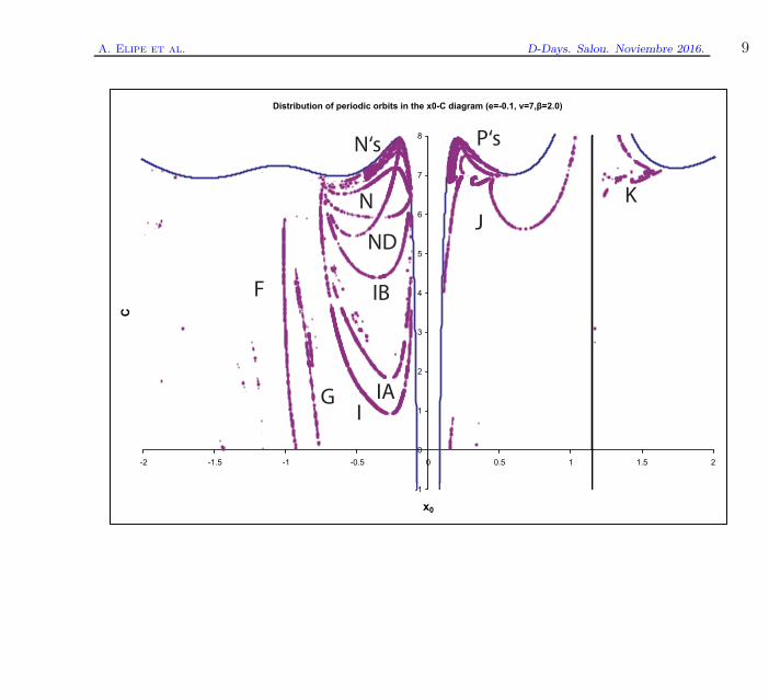
A. Elipe et al. D-Days. Salou. Noviembre 2016. 9
Distribution of periodic orbits in the x0-C diagram (e=-0.1, =7, =2.0)
-1
0
1
2
3
4
5
6
7
8
-2 -1.5 -1 -0.5 0 0.5 1 1.5 2
x0
C
F
GI
IA
IB
N
ND
J
K
P‘sN‘s

A. Elipe et al. D-Days. Salou. Noviembre 2016. 10
Distribution of periodic orbits in the x0-C diagram (e=-0.14, =7, =2.0)
0
1
2
3
4
5
6
7
8
9
-2,6 -1,6 -0,6 0,4 1,4 2,4
x0
C
groups NUand ND
groups PUand PD
J
K
I
IA
IB
F
G
ND

A. Elipe et al. D-Days. Salou. Noviembre 2016. 11
Distribution of periodic orbits in the x0-C diagram (e=-0.3, =7, =2.0)
-5
-3
-1
1
3
5
7
9
11
-3 -2 -1 0 1 2 3
x0
C
J
K
F
I
G
A. Elipe et al. D-Days. Salou. Noviembre 2016. 12
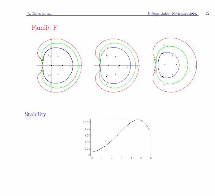
Family F
-1 1 2 3
-2
-1
1
2
-1 1 2 3
-2
-1
1
2
-1 1 2 3
-2
-1
1
2
Stability
0 1 2 3 4 5 60
200
400
600
800
1000

A. Elipe et al. D-Days. Salou. Noviembre 2016. 13
Family G
-1 -0.5 0.5 1
-1.5
-1
-0.5
0.5
1
1.5
-1 -0.5 0.5 1
-1.5
-1
-0.5
0.5
1
1.5
-1 -0.5 0.5 1
-1.5
-1
-0.5
0.5
1
1.5
Stability
2 2.5 3 3.5 4 4.50
2000
4000
6000
8000
10000
A. Elipe et al. D-Days. Salou. Noviembre 2016. 14
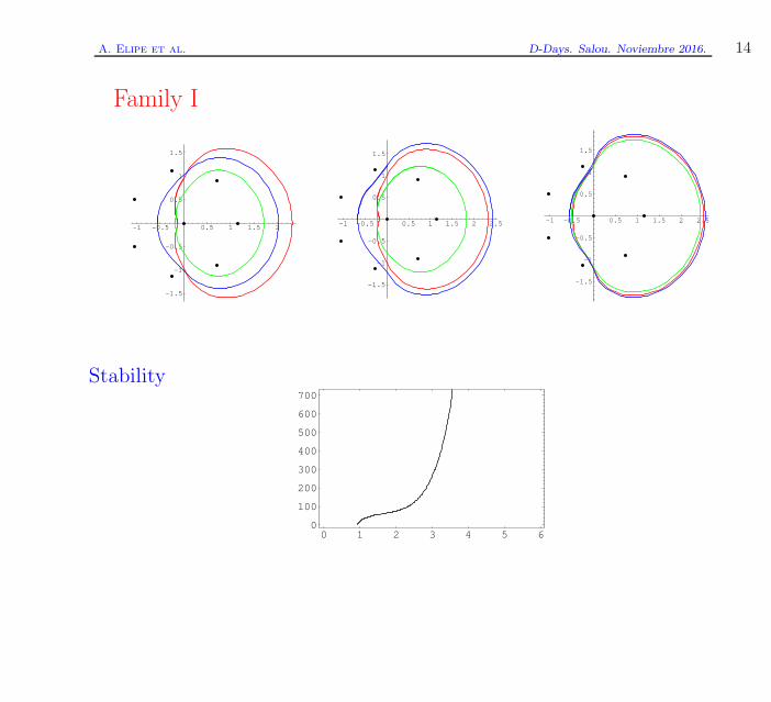
Family I
-1 -0.5 0.5 1 1.5 2
-1.5
-1
-0.5
0.5
1
1.5
-1 -0.5 0.5 1 1.5 2 2.5
-1.5
-1
-0.5
0.5
1
1.5
-1 -0.5 0.5 1 1.5 2 2.5
-1.5
-1
-0.5
0.5
1
1.5
Stability
0 1 2 3 4 5 60
100
200
300
400
500
600
700
A. Elipe et al. D-Days. Salou. Noviembre 2016. 15
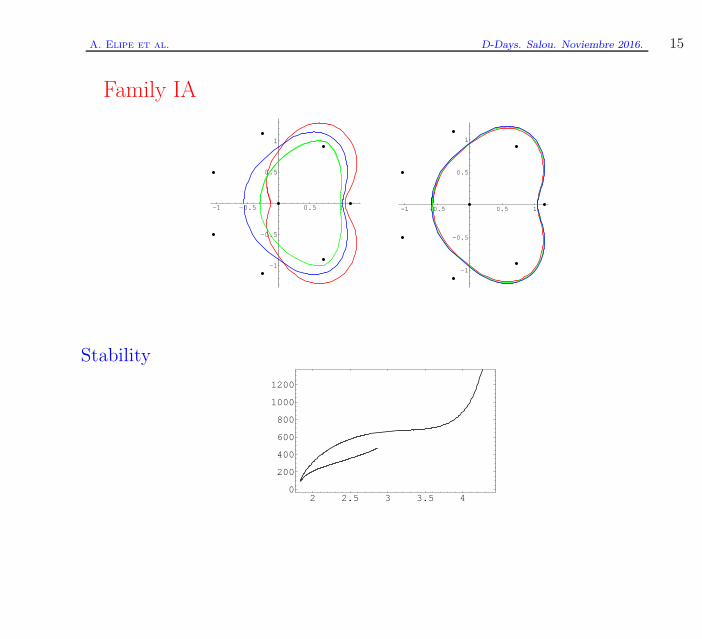
Family IA
-1 -0.5 0.5 1
-1
-0.5
0.5
1
-1 -0.5 0.5 1
-1
-0.5
0.5
1
Stability
2 2.5 3 3.5 40
200
400
600
800
1000
1200
A. Elipe et al. D-Days. Salou. Noviembre 2016. 16
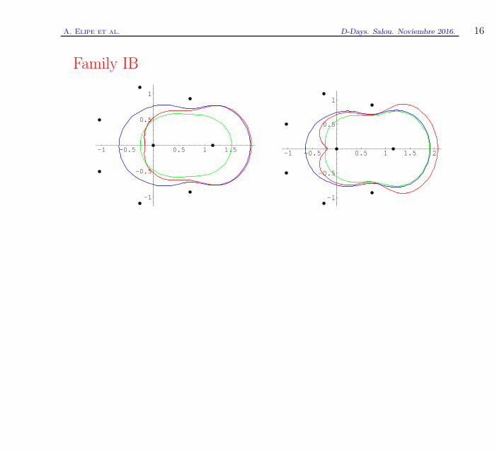
Family IB
-1 -0.5 0.5 1 1.5
-1
-0.5
0.5
1
-1 -0.5 0.5 1 1.5 2
-1
-0.5
0.5
1
A. Elipe et al. D-Days. Salou. Noviembre 2016. 17
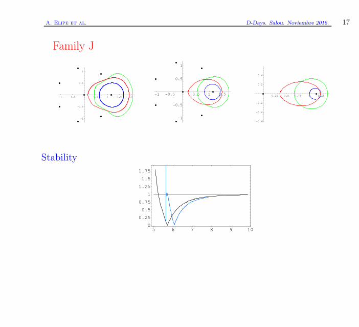
Family J
-1 -0.5 0.5 1 1.5 2
-1
-0.5
0.5
1
-1 -0.5 0.5 1 1.5
-1
-0.5
0.5
1
0.25 0.5 0.75 1 1.25
-0.6
-0.4
-0.2
0.2
0.4
Stability
5 6 7 8 9 100
0.25
0.5
0.75
1
1.25
1.5
1.75
A. Elipe et al. D-Days. Salou. Noviembre 2016. 18
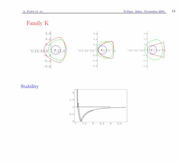
Family K
0.40.60.8 1.21.4
-0.6
-0.4
-0.2
0.2
0.4
0.6
0.4 0.6 0.8 1.2 1.4 1.6
-0.6
-0.4
-0.2
0.2
0.4
0.6
0.4 0.6 0.8 1.2 1.4 1.6
-0.6
-0.4
-0.2
0.2
0.4
0.6
Stability
7 7.5 8 8.5 9 9.50
0.5
1
1.5
2
A. Elipe et al. D-Days. Salou. Noviembre 2016. 19
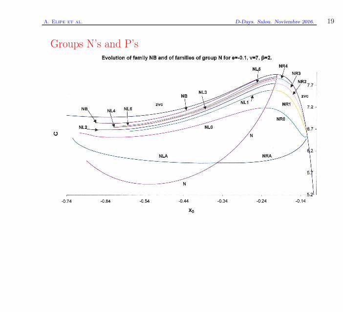
Groups N’s and P’s
A. Elipe et al. D-Days. Salou. Noviembre 2016. 20
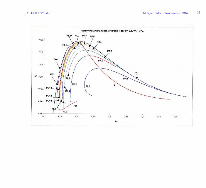
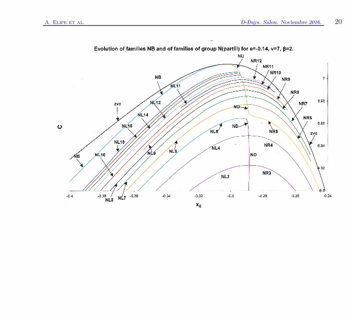
A. Elipe et al. D-Days. Salou. Noviembre 2016. 21
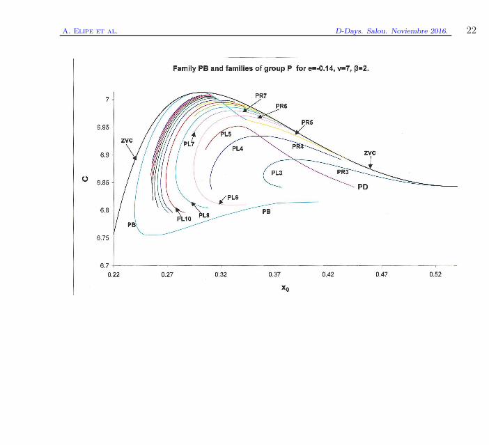
A. Elipe et al. D-Days. Salou. Noviembre 2016. 22

A. Elipe et al. D-Days. Salou. Noviembre 2016. 23
Families N and NB
-1 -0.5 0.5 1
-1
-0.5
0.5
1
-0.5 -0.4 -0.3 -0.2
-0.2
-0.15
-0.1
-0.05
0.05
0.1
0.15
0.2
-0.7 -0.6 -0.5 -0.4 -0.3 -0.2 -0.1
-0.2
-0.1
0.1
0.2
A. Elipe et al. D-Days. Salou. Noviembre 2016. 24
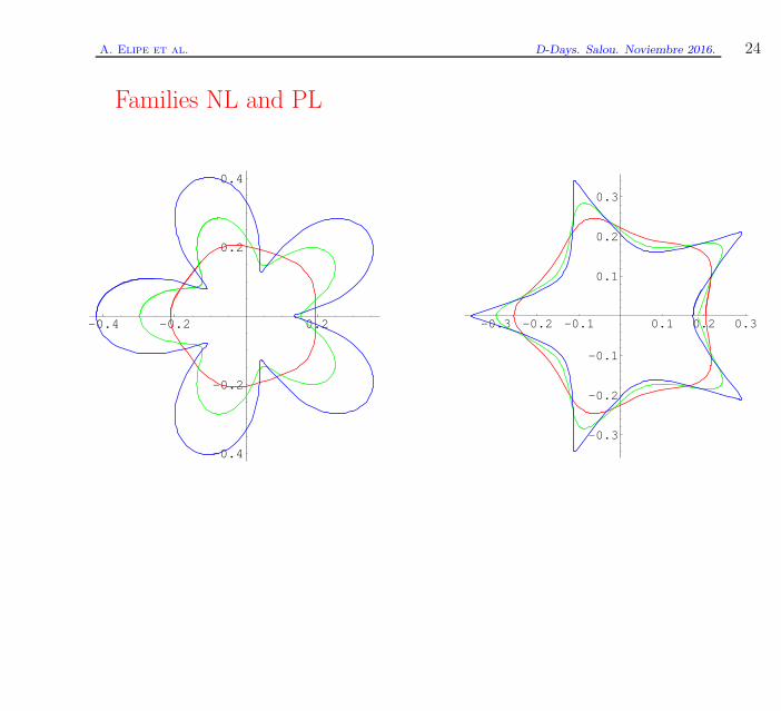
Families NL and PL
-0.4 -0.2 0.2
-0.4
-0.2
0.2
0.4
-0.3 -0.2 -0.1 0.1 0.2 0.3
-0.3
-0.2
-0.1
0.1
0.2
0.3

A. Elipe et al. D-Days. Salou. Noviembre 2016. 25
Stability
5.9 6 6.1 6.2 6.3
0.5
1
1.5
2
2.5
A. Elipe et al. D-Days. Salou. Noviembre 2016. 26
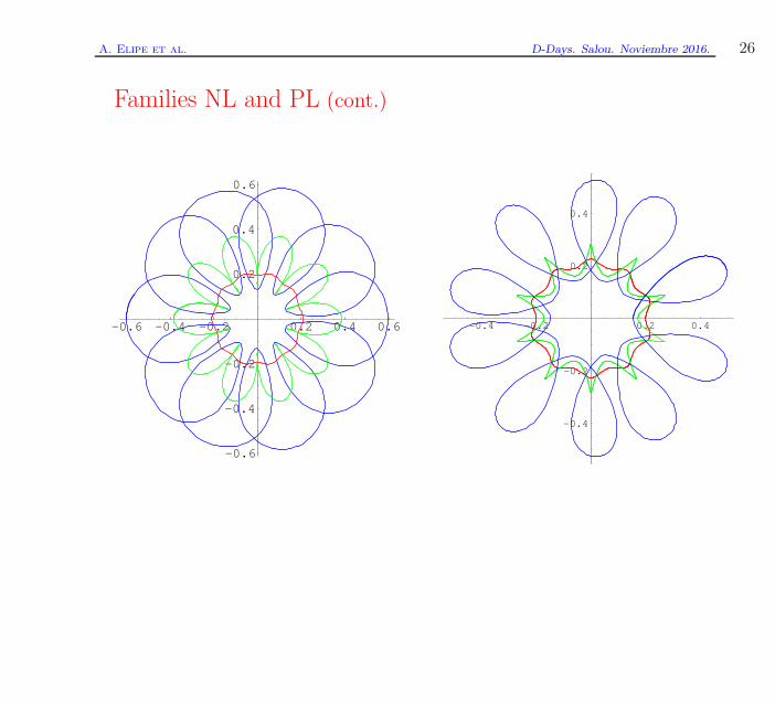
Families NL and PL (cont.)
-0.6 -0.4 -0.2 0.2 0.4 0.6
-0.6
-0.4
-0.2
0.2
0.4
0.6
-0.4 -0.2 0.2 0.4
-0.4
-0.2
0.2
0.4
A. Elipe et al. D-Days. Salou. Noviembre 2016. 27
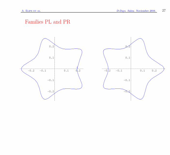
Families PL and PR
-0.2 -0.1 0.1 0.2
-0.2
-0.1
0.1
0.2
-0.2 -0.1 0.1 0.2
-0.2
-0.1
0.1
0.2