dynamics me 34010 - meeng.technion.ac.il
TRANSCRIPT

DYNAMICS
ME 34010
Prof. M. B. Rubin
Prof. E. Altus
Faculty of Mechanical Engineering
Technion - Israel Institute of Technology
Fall 1992
Latest revision April 2008
2
Table of Contents
1. Introduction ............................................................................................................ 4
2. Vector Algebra And Indicial Notation..................................................................... 6
3. Vector Calculus..................................................................................................... 16
4. Position, Velocity, Acceleration ............................................................................ 19
5. Tangential And Normal Coordinates ..................................................................... 21
6. Rectilinear Motion ................................................................................................ 26
7. Polar Coordinates.................................................................................................. 29
8. Cylindrical Polar Coordinates................................................................................ 32
9. Relative Motion .................................................................................................... 34
10. Rotating Coordinate Axes And Angular Velocity.................................................. 36
11. General Differential Operator................................................................................ 39
12. Spherical Polar Coordinates .................................................................................. 43
13. General Rigid Body Motion .................................................................................. 46
14. Instantaneous Screw Motion Of A Rigid Body...................................................... 50
15. Contact of Bodies.................................................................................................. 53
16. Kinetics Of A Particle ........................................................................................... 57
17. Vibrations ............................................................................................................. 63
18. Mechanical Power, Work and Energy (Particle) .................................................... 72
19. Conservative Force Fields ..................................................................................... 75
20. Energy Equation For A Particle............................................................................. 83
21. Angular Momentum.............................................................................................. 85
22. Conservation Of Momentum (?)............................................................................ 87
23. Impulse And Momentum (Systems Of Particles) ................................................... 90
24. Kinetics Of Systems Of Particles........................................................................... 94
25. Alternative Formulation of the Balance Laws........................................................ 99
26. Impulse And Momentum (System Of Particles)................................................... 103
27. Mechanical Power And Kinetic Energy (Systems Of Particles) ........................... 104
28. Impact of two particles........................................................................................ 107
29. Equations Of Motion Of A Rigid Body ............................................................... 118
30. Inertia Tensor...................................................................................................... 124
3
31. Transfer Theorem For The Inertia Tensor............................................................ 135
32. Planar Motion ..................................................................................................... 139
33. Impulse On A Rigid Body................................................................................... 142
34. Energy Equation For A Rigid Body..................................................................... 145
35. Angular Momentum And Transformation Relations ............................................ 149
36. Point Masses, Massless Links, And A System Of Rigid Bodies ........................... 153
37. Gyroscopic Effects.............................................................................................. 165
38. Euler Angles And A Spinning Top...................................................................... 169
39. Euler Equations Of Motion ................................................................................. 177

4
1. Introduction
Sir Issac Newton (1642-1727) was the first to discover the correct laws of motion of
particles. Since then much work has been done to verify the validity of these laws and to
generalize them for deformable media. The study of rigid body dynamics is concerned
with developing and analyzing the equations of motion of: a single particle, a system of
particles, a rigid body, and a system of rigid bodies.
To analyze the motion of a particle it is necessary to first develop kinematical
expressions for the position, velocity and acceleration of the particle. Then, it is
necessary to consider the kinetic equations of motions which characterize the influence of
the forces applied to the particle on its motion. Thus, the analysis of both kinematics and
kinetics are necessary for a complete formulation of a specific problem. Since the
analysis of the motion of a single particle is simpler than that of a rigid body, most
courses in dynamics develop the material in the following order. The kinematics and
kinetics of motion of a single particle are discussed for the simplest case of motion in a
straight line. Then, the equations are generalized to motion in a plane followed by
motion in three-dimensional space. Next, the kinematics and kinetics of motion of a
system of particle is developed. The analysis of rigid body motion starts with analysis in
a plane and then is concluded with analysis in three-dimensional space. This approach
has the advantage that mathematical complexity increases gradually and that physical
concepts are presented in their simplest forms. However, it has the disadvantage that the
more complicated mathematical tools required to analyze general three-dimensional
motion are presented near the end of the course when there is often not sufficient time to
fully absorb the material.
This course in dynamics presents the material in a different order from that in a
standard presentation. The course is loosely separated into two parts. Part 1 includes
sections 2-15 which develop the analysis of kinematics in three-dimensions and Part 2
includes sections 16-39 which introduce the kinetic equations of motion to analyze forces
and energies of systems of rigid bodies. This approach has the advantage that the more
complicated mathematical tools of analyzing motion in rotating coordinate systems is
developed in Part 1. Since the analysis of the kinetics of particles and rigid bodies
necessarily requires the determination of acceleration, the more complicated

5
mathematical tools for analyzing motion in three-dimensions are used in almost all
example problems in Part 2. This ensures that these mathematical tools are fully
absorbed. Moreover, it ensures that at the end of the course each student can confidently
formulate even the most complicated dynamics problems in three-dimensions.

6
2. Vector Algebra and Indicial Notation
In mechanics it is necessary to use vectors and vector equations to express physical
laws. To conveniently express the component forms of these vector equations it is
desirable to use a language called indicial notation which develops simple rules
governing manipulations of the components of these vector equations. For the purposes
of describing this language we introduce a set of right-handed orthonormal base vectors
denoted by (e1,e2,e3), such that
e1 • e1 = 1 , e2 • e2 = 1 , e3 • e3 = 1 , (2.1a,b,c)
e1 • e2 = 0 , e1 • e3 = 0 , e2 • e3 = 0 , (2.1d,e,f)
e1 × e2 = e3 , e3 × e1 = e2 , e2 × e3 = e1 , (2.1g,h,i)
where e1 • e2 denotes the dot product between the two vectors, and e1 × e2 denotes the
cross product between the two vectors. In this text we will use a bold faced symbol like a
to indicate a vector quantity and in the written form we will use a wavy line under the
symbol like ~ a to indicate the same vector quantity a.
VECTOR ALGEBRA
Rules of Vector Addition and Multiplication by a Scalar: Let a, b , and c be vectors
and α and β be scalars. Then the commutative and associative laws of vector addition are
(see Fig. 2.1)
a + b = b + a (commutative law) , (2.1a)
a + (b + c) = (a + b) + c (associative law) , (2.1b)
Furthermore, the associative laws of scalar multiplication may be summarized as
α (β a) = (αβ) a = β (α a) = a (α β) , (2.2a)
(α + β) a = α a + β a , (2.2b)
α (a + b) = α a + α b . (2.2c)

7
a
b
a
ba + b
b + a
Fig. 2.1
Components of a Vector: An arbitrary vector a in Euclidean three-dimensional space
may be expressed in terms of its components {a1,a2,a3} relative to the fixed base vectors
{e1,e2,e3} such that
a = a1 e1 + a2 e2 + a3 e3 . (2.3)
Scalar (Dot) Product: Magnitude and Direction of a Vector: The scalar (or dot)
product between two vectors a and b is defined by
a • b = (a1 e1 + a2 e2 + a3 e3) • (b1 e1 + b2 e2 + b3 e3)
= a1b1 + a2b2 + a3b3 , (2.4)
where {b1,b2,b3} are the components of b relative to the base vectors {e1,e2,e3}. It
follows that the magnitude a and the unit direction ea of vector a may be defined by
a = | a | = (a • a)1/2 = (a12 + a2
2 + a32)1/2 , (2.5a)
ea = aa =
a1a e1 +
a2a e2 +
a2a e2 , ea • ea = 1 , (2.5b,c)
so that a may be represented in the form
a = a ea . (2.6)
The scalar product a • b may also be written in the more physical form
a • b = a b cosθ , (2.7a)
a • b = a (b • ea) = a (b cosθ) , a • b = b (a • eb) = b (a cosθ) , (2.7b,c)
where θ is the angle between a and b (see Fig. 2.2). The representation (2.7b) expresses
a • b as the magnitude of a times the projection of b in the direction of a, whereas the

8
representation (2.7c) expresses a • b as the magnitude of b times the projection of a in the
direction of b. Furthermore, we note that the scalar product is commutative so that
a • b = b • a . (2.8)
a
b
!
b cos !
a
b
!
a cos !
Fig. 2.2
Also, it follows that the components of a may be calculated by using the scalar product
by
a1 = a • e1 , a2 = a • e2 , a3 = a • e3 . (2.9a,b,c)
Defining {θ1,θ2,θ3} as the angles between the vector a and the base vectors {e1,e2,e3},
respectively, the components of the direction vector ea in (2.5b) may be represented by
(see Fig. 2.3)
a1a = cosθ1 ,
a2a = cosθ2 ,
a3a = cosθ3 . (2.10a,b,c)
a
e1
e2
e3
1!
2!
3!
Fig. 2.3
9
Vector (Cross) Product: The vector product between the two vectors a and b may be
calculated directly using the expressions (2.1g,h,i) or may be calculated using the
determinant of a matrix of the form
a × b = ⎪⎪⎪⎪
⎪⎪⎪⎪e1 e2 e3
a1 a2 a3b1 b2 b3
, (2.11a)
= (a2b3 – a3b2) e1 – (a1b3 – a3b1) e2 + (a1b2 – a2b1) e3 . (2.11b)
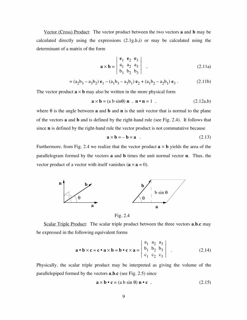
The vector product a × b may also be written in the more physical form
a × b = (a b sinθ) n , n • n = 1 , (2.12a,b)
where θ is the angle between a and b and n is the unit vector that is normal to the plane
of the vectors a and b and is defined by the right-hand rule (see Fig. 2.4). It follows that
since n is defined by the right-hand rule the vector product is not commutative because
a × b = – b × a . (2.13)
Furthermore, from Fig. 2.4 we realize that the vector product a × b yields the area of the
parallelogram formed by the vectors a and b times the unit normal vector n. Thus, the
vector product of a vector with itself vanishes (a × a = 0).
!
a
bn
a
b
!
b sin !
Fig. 2.4
Scalar Triple Product: The scalar triple product between the three vectors a,b,c may
be expressed in the following equivalent forms
a • b × c = c • a × b = b • c × a = ⎪⎪⎪⎪
⎪⎪⎪⎪a1 a2 a3
b1 b2 b3c1 c2 c3
. (2.14)
Physically, the scalar triple product may be interpreted as giving the volume of the
parallelepiped formed by the vectors a,b,c (see Fig. 2.5) since
a × b • c = (a b sin θ) n • c , (2.15)

10
where (a b sin θ) is the area of the base of the parallelepiped and n • c is the height of the
parallelepiped.
a
bc
n
!
Fig. 2.5
Note that the order of the scalar and vector product may be interchanged without
changing the value of the scalar triple product. This can also be seen by realizing that the
volume of the parallelepiped in Fig. 2.5 can be obtained by expressing the scalar triple
product in terms of the vector product of an two of the three vectors a,b,c whose normal
n (according to the right-hand rule) points toward the interior of the parallelepiped.
Vector Triple Product: The vector triple product between the three vectors a,b,c may
be expanded in the form
a × (b × c) = (a • c) b – (a • b) c . (2.16)
It is important to emphasize that since the vector product between two vectors generates
another vector it is essential to include parentheses in the definition (2.16). Also note that
the vector a × (b × c) is perpendicular to the vector (b × c). But the vector (b × c) is
perpendicular to the plane formed by b and c. This means that the vector a × (b × c)
must lie in the plane of b and c, which is consistent with the result (2.16). Furthermore,
the vector a × (b × c) must also be perpendicular to a, which is consistent with the result
(2.16).

11
INDICIAL NOTATION
Quantities written in indicial notation will have a finite number of indices attached to
them. Since the number of indices can be zero a quantity with no index can also be
considered to be written in index notation. The language of indicial notation is quite
simple because only two types of indices may appear in any term. Either the index is a
free index or it is a repeated index. Also, we will define a simple summation convention
which applies only to repeated indices. These two types of indices and the summation
convention are defined as follows.
Free Indices: Indices that appear only once in a given term are known as free indices.
For our purposes each of these free indices will take the values (1,2,3). For example, i is
a free index in each of the following expressions
(x1 , x2 , x3 ) = xi (i=1,2,3) , (2.17a)
(e1 , e2 , e3 ) = ei (i=1,2,3) . (2.17b)
Notice that the free index i in (2.17) refers to the group of three quantities defined by i
taking the values 1,2,3.
Repeated Indices: Indices that appear twice in a given term are known as repeated
indices. For example i and j are free indices and m and n are repeated indices in the
following expressions
ai bj cm Tmn dn , Aimmjnn , Aimn Bjmn . (2.18a,b,c)
It is important to emphasize that in the language of indicial notation an index can never
appear more than twice in any term.
Einstein Summation Convention: When an index appears as a repeated index in a
term, that index is understood to take on the values (1,2,3) and the resulting terms are
summed. Thus, for example,
xi ei = x1 e1 + x2 e2 + x3 e3 . (2.19)
Because of this summation convention, repeated indices are also known as dummy
indices since their replacement by any other letter not appearing as a free index and also
not appearing as another repeated index does not change the meaning of the term in
which they occur. For examples,
xi ei = xj ej , ai bmcm = ai bj cj . (2.20a,b)

12
It is important to emphasize that the same free indices must appear in each term in an
equation so that for example the free index i in (2.20b) must appear on each side of the
equation.
Kronecker Delta: The Kronecker delta symbol δij is defined by
δij = ei • ej = ⎩⎪⎨⎪⎧ 1 if i = j 0 if i ≠ j . (2.21)
Since the Kronecker delta δij vanishes unless i=j it exhibits the following exchange
property
δij xj = ( δ1j xj , δ2j xj , δ3j xj ) = ( x1 , x2 , x3 ) = xi . (2.22)
Notice that the Kronecker symbol may be removed by replacing the repeated index j in
(2.22) by the free index i.
Recalling that an arbitrary vector a in Euclidean 3-Space may be expressed as a linear
combination of the base vectors ei such that
a = ai ei , (2.23)
it follows that the components ai of a can be calculated using the Kronecker delta
ai = ei • a = ei • (am em) = (ei • em) am = δim am = ai . (2.24)
Notice that when the expression (2.23) for a was substituted into (2.24) it was necessary
to change the repeated index i in (2.23) to another letter (m) because the letter i already
appeared in (2.24) as a free index. It also follows that the Kronecker delta may be used to
calculate the dot product between two vectors a and b with components ai and bi,
respectively by
a • b = (ai ei) • (bj ej) = ai (ei • ej) bj = ai δij bj = ai bi . (2.25)
Contraction: Contraction is the process of identifying two free indices in a given
expression together with the implied summation convention. For example we may
contract on the free indices i,j in δij to obtain
δii = δ11 + δ22 + δ33 = 3 . (2.26)
Note that contraction on the set of 9=32 quantities Tij can be performed by multiplying
Tij by δij to obtain

13
Tij δij = Tii = T11 + T22 + T33. (2.27)
Matrix Multiplication: In order to connect the summation convention with standard
matrix multiplication consider two vectors with components ai,bi, and three square
matrices with components Aij,Bij,Cij and define
bi = Aij aj , Cij = AimBmj . (2.28a,b)
Since the first index of Aij indicates the row and the second index indicates the column, it
can easily be seen that the summation on the index j in (2.28a) yields the same result of
the multiplication of the matrix Aij with the column vector aj to obtain the column vector
bi. Similarly, since the second index of Aim in (2.28b) is summed with the first index of
Bmj it is easy to see that Cij is the matrix that is obtained by multiplying the matrix Aim
with the matrix Bmj.
Transpose: Let Aij be the components of a matrix A. Then the components of the
transpose AT of A are given by
(AT)ij = AijT = Aji . (2.29)
In the above we have considered terms that have no free indices like in equations
(2.19), (2.20a), (2.23), (2.25)-(2.27); that have one free index like in equations (2.22),
(2.24), (2.28a); and that have two free indices like in equations (2.18), (2.21), (2.28b),
(2.29). Obviously, it is possible to write terms that have any number of free indices. In
general, a term is said to be of order zero if it has no free index, of order one if it has one
free index and of order n if it has n free indices. Usually in mechanics terms with indices
are components of quantities called tensors, which are generalizations of vectors. In
particular, when a and b are vectors the quantity a • b in (2.25) is called a scalar or zero
order tensor (or a tensor of order zero). Also, the quantities ai in (2.24) are the
components of the vector a, which is also called a first order tensor (or a tensor of order
one). In this course we will consider tensors up to order three.

14
Permutation Symbol: The permutation symbol εijk is defined by
+ 1 for (i,j,k) equal to an even permutation of (1,2,3),
(i,j,k) = (1,2,3), (3,1,2), (2,3,1)
εijk = ei × ej • ek = – 1 for (i,j,k) equal to an odd permutation of (1,2,3),
(i,j,k) = (1,3,2), (2,1,3), (3,2,1)
0 whenever any of the indices (i,j,k) are, repeated more than
once (i.e i=j, or i=k, or j=k, or i=j=k)
(2.30)
It can be shown that the nine vectors ei × ej can be expressed in terms of the permutation
symbol using the expression
ei × ej = εijk ek . (2.31)
Thus, the vector product between the two vectors a and b may be expressed in the form
a × b = ai ei × bj ej = εijk ai bj ek . (2.32)
For convenience we summarize the expanded and short forms of a number of vector
quantities in Table 2.1.

15
Quantity Expanded Form Short Form
Rectangular Cartesian Coordinates
x1,x2,x3 xi (i=1,2,3)
Rectangular Cartesian Base Vectors
e1,e2,e3 ei
Position Vector x = x1 e1 + x2 e2 + x3 e3 xi ei
Components of Vector a a1 = a • e1 , a2 = a • e2 a3 = a • e3
ai = a • ei
Vector a a = a1 e1 + a2 e2 + a3 e3 a = ai ei Scalar Product a • b = a1b1 + a2b2 + a3b3 a • b = ai bi
Vector Product a × b = (a2b3 – a3b2) e1 + (a3b1 – a1b3) e2 + (a1b2 – a2b1) e3
a × b = εijk ai bj ek
Gradient of a Scalar φ ∇ φ =
∂φ∂x1
e1 + ∂φ∂x2
e2
+ ∂φ∂x3
e3 ∇ φ =
∂φ∂xi
ei
Divergence of a Vector a ∇ • a = ∂a1∂x1
+ ∂a2∂x2
+ ∂a3∂x3
∇ • a = ∂ai∂xi
Curl of a Vector a
∇ × a = ⎝⎜⎛
⎠⎟⎞∂a3
∂x2 – ∂a2∂x3
e1
+ ⎝⎜⎛
⎠⎟⎞∂a1
∂x3 – ∂a3∂x1
e2
+ ⎝⎜⎛
⎠⎟⎞∂a2
∂x1 – ∂a1∂x2
e3
∇ × a = εijk ∂aj∂xi
ek
Table 2.1

16
3. Vector Calculus
In dynamics most vectors will be considered to be functions of time t and many of the
equations in dynamics will be differential equations that need to be integrated.
Consequently, it is important to learn how to differentiate and integrate vector functions.
Differentiation: To this end, we define the time derivative of the vector function a(t)
by the same limiting process that derivatives of scalar functions are defined
dadt = •a =
limitΔt → 0
a(t+Δt) – a(t)Δt . (3.1)
In (3.1) and throughout the text we use the notation da/dt and a superposed (•) to denote
time differentiation. It is important to note that both the magnitude and direction of a
vector can change with time (see Fig. 3.1).
a(t)
a(t+!t)a(t+!t) – a(t)
Fig.3.1
The standard rules of differentiation of scalar functions apply to vector functions except
that the commutative law does not apply to the vector product between two vectors. It
follows that if a and b are vector functions of time and α is a scalar function of time that
ddt (a + b) =
dadt +
dbdt , (3.2a)
ddt (α a) =
dαdt a + α
dadt , (3.2b)
ddt (a • b) =
dadt • b + a •
dbdt , (3.2c)
ddt (a × b) =
dadt × b + a ×
dbdt . (3.2d)
Vector of Constant Magnitude: Since we usually refer vectors to base vectors that
have unit length it is desirable to consider the derivative of a general vector a of constant
magnitude. Thus, let

17
a • a = constant . (3.3)
Taking the derivative of (3.3) we have
•a • a + a • •a = 2 a • •a = 0 , (3.4)
which means that •a is perpendicular to a (see Fig. 3.2) so that the vector a can only
rotate.
a
a•
Fig. 3.2
Indefinite Integral of a Vector: The indefinite integral of the vector function f(t) is
denoted by
∫t f(τ) dτ , (3.5)
where the lower limit of integration is understood to be any arbitrary fixed value and τ is
merely a variable of integration. It follows that (3.5) denotes all functions whose
derivative is f, so that
ddt ∫
t f(τ) dτ = f(t) . (3.6)
Definite Integral of a Vector: The definite integral of a vector function f(t) from time
t0 to time t is denoted by
∫ tt0
f(τ) dτ . (3.7)
Integral of a Vector Differential Equation: Consider the vector differential equation
given by
dFdt = f(t) . (3.8)
Integrating (3.8) using the indefinite integral (3.5) we deduce that
F(t) = ∫t f(τ) dτ + C , (3.9)

18
where C is an arbitrary constant vector. Now in order to determine the function F(t)
uniquely we need to specify the initial value of F [say F(t0)]. Thus, with the help of this
initial condition we may determine the value of C in (3.9) by the equation
F(t0) = ∫t0 f(τ) dτ + C . (3.10)
Now substituting (3.10) into (3.9) we deduce that
F(t) = F(t0) + ∫ tt0
f(τ) dτ , (3.11)
where we have used the fact that
∫ tt0
f(τ) dτ = ∫t f(τ) dτ – ∫t0 f(τ) dτ . (3.12)
Finally, we note that the integral of the sum of two vector functions a,b is equal to the
sum of the integrals of the functions
∫ (a + b) dt = ∫ a dt + ∫ b dt . (3.13)

19
4. Position, Velocity, Acceleration
Let x(t) be the position vector relative to a fixed origin of a point that moves in space
along a curve C (see Fig. 4.1). The average velocity vavg over the time period [t,t+Δt] is
defined by
vavg = x(t+Δt) – x(t)
Δt , (4.1)
and the velocity (instantaneous velocity) v is defined as the derivative of the position
vector
v(t) = •x(t) = limitΔt →0
x(t+Δt) – x(t)Δt . (4.2)
Fig. 4.1
Note from Fig. 4.1 that in the limit that Δt approaches zero the vector x(t+Δt)–x(t)
becomes tangent to the curve C so the instantaneous velocity v is always tangent to the
path traversed by the point. Furthermore, the acceleration a of a point is defined as the
derivative of the velocity so that
a = •v = limitΔt →0
v(t+Δt) – v(t)Δt = ••x . (4.3)
The displacement of a point from the position x(t1) at time t1 to its position x(t2) at
time t2 may be obtained by integrating the velocity v
x(t2) – x(t1) = ∫t2t1 v(τ) dτ . (4.4)
e1 e2
e3
x(t+Δt)
x(t)
x(t+Δt)–x(t)
v(t) C

20
Also, the distance traveled along the path traversed by the point is an increasing function
of t so the distance traveled from time t1 to time t2 is calculated by integrating the
magnitude of the velocity v and is denoted by D2/1
D2/1 =∫t2t1 | v(τ) | dτ . (4.5)
21
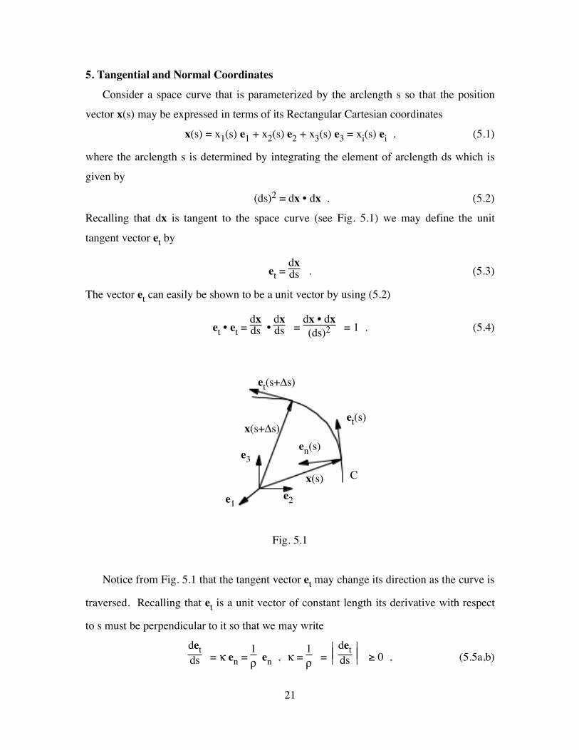
5. Tangential and Normal Coordinates
Consider a space curve that is parameterized by the arclength s so that the position
vector x(s) may be expressed in terms of its Rectangular Cartesian coordinates
x(s) = x1(s) e1 + x2(s) e2 + x3(s) e3 = xi(s) ei , (5.1)
where the arclength s is determined by integrating the element of arclength ds which is
given by
(ds)2 = dx • dx , (5.2)
Recalling that dx is tangent to the space curve (see Fig. 5.1) we may define the unit
tangent vector et by
et = dxds . (5.3)
The vector et can easily be shown to be a unit vector by using (5.2)
et • et = dxds •
dxds =
dx • dx(ds)2 = 1 . (5.4)
Fig. 5.1
Notice from Fig. 5.1 that the tangent vector et may change its direction as the curve is
traversed. Recalling that et is a unit vector of constant length its derivative with respect
to s must be perpendicular to it so that we may write
detds = κ en =
1ρ en , κ =
1ρ = ⎪⎪
⎪⎪⎪⎪
detds ≥ 0 , (5.5a,b)
e1 e2
e3
x(s+Δs)
x(s) C
et(s)
et(s+Δs)
en(s)

22
where κ is the curvature and ρ is the radius of curvature of the space curve. Note that
since κ is nonnegative the vector en points towards the inside of the space curve (see Fig.
5.1).
To help understand the curvature consider the special case of a planar curve for which
x(s) = x1(s) e1 + x2(s) e2 . (5.6)
Furthermore, let Δψ be the angle between the tangent vector et(s) at s and the tangent
vector et(s+Δs) at s+Δs (see Fig. 5.2). It follows from geometry that the vector et(s+Δs)
may be expressed in terms of the base vectors et(s) and en(s) at s such that
et(s+Δs) = cosΔψ et(s) + sinΔψ en(s) . (5.7)
te (s)
e (s)n
te (s)
e (s)n
e (s+!s)t
e (s+!s)t
!"
Fig. 5.2
Recalling the definition of the derivative we have
detds =
limitΔs → 0
et(s+Δs) – et(s)Δs , (5.8a)
= limitΔs → 0 ⎣
⎢⎡
⎦⎥⎤
⎝⎜⎛
⎠⎟⎞cosΔψ – 1
Δs et(s) + ⎝⎜⎛
⎠⎟⎞sinΔψ
Δs en(s) . (5.8b)
But using the Taylor series expansions of cosΔψ and sinΔψ
cosΔψ ≈ 1 – (Δψ)2
2 + ... , sinΔψ ≈ Δψ – (Δψ)3
6 + ... , (5.9a,b)
we may rewrite (5.8b) in the form
detds =
limitΔs → 0 ⎣
⎢⎡
⎦⎥⎤
– (Δψ)2
2Δs et(s) + ⎝⎜⎛
⎠⎟⎞Δψ
Δs en(s) = dψds en(s) . (5.10)
23
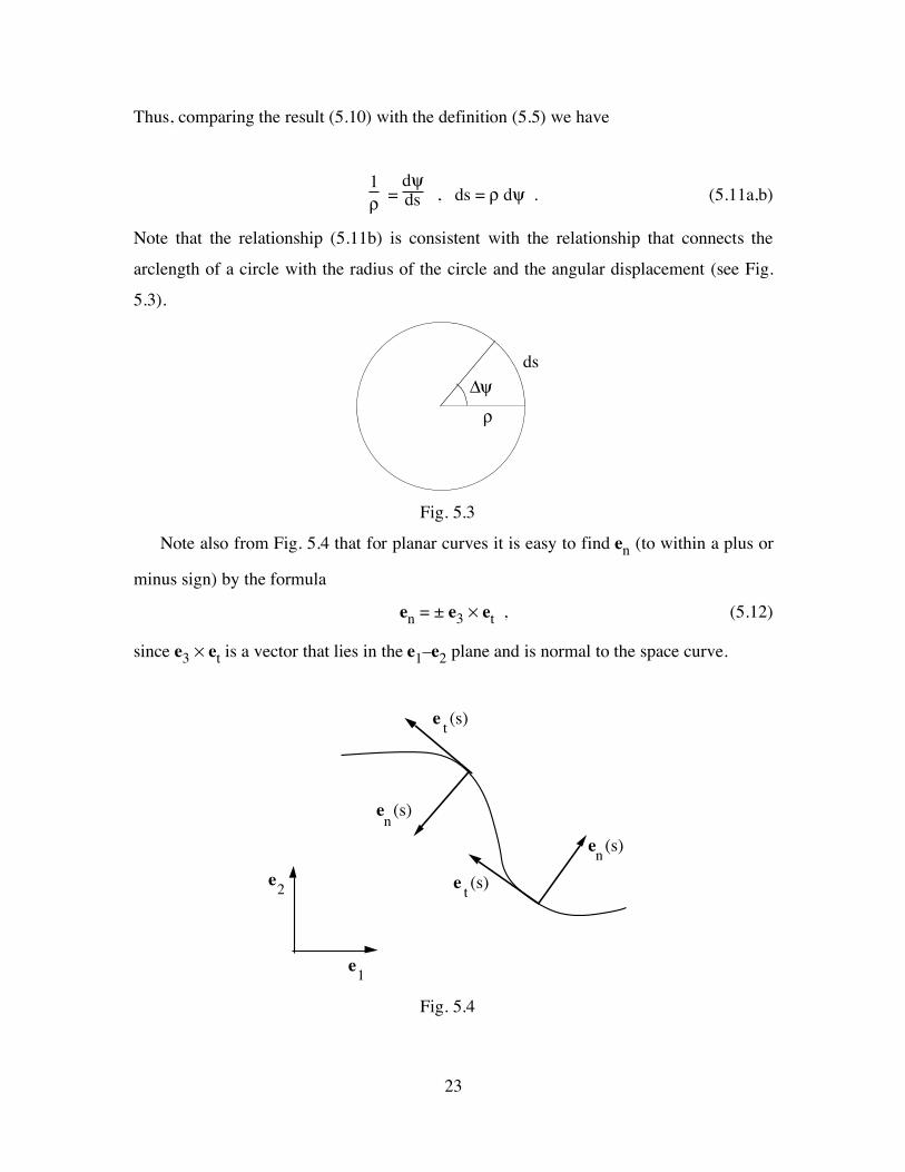
Thus, comparing the result (5.10) with the definition (5.5) we have
1ρ =
dψds , ds = ρ dψ . (5.11a,b)
Note that the relationship (5.11b) is consistent with the relationship that connects the
arclength of a circle with the radius of the circle and the angular displacement (see Fig.
5.3).
!"
#
ds
Fig. 5.3
Note also from Fig. 5.4 that for planar curves it is easy to find en (to within a plus or
minus sign) by the formula
en = ± e3 × et , (5.12)
since e3 × et is a vector that lies in the e1–e2 plane and is normal to the space curve.
te (s)
e (s)n
te (s)
e (s)n
e1
e2
Fig. 5.4

24
For some problems it is convenient to use tangential and normal coordinates to
describe motion of a particle moving in space. Within this context, the position vector x
depends on time parametrically through the specification of s(t) so that
x = x(s(t)) . (5.13)
Thus, with the help of (5.3) and (5.5a) we may use the chain rule of differentiation to
calculate the velocity v and acceleration a in the forms
v = •x = dxds •s = •s et , (5.14a)
a = •v = ••s et + •s •et = ••s et + •s 2 detds = ••s et +
•s2
ρ en . (5.14b)
It follows that the tangential and normal components of the velocity and acceleration
become
vt = v • et = •s the component of the velocity tangent to the curve defining
the path of motion
vn = v • en = 0 the velocity is always tangent to the path of motion
at = a • et = ••s the component of acceleration tangent to the curve
an = a • en = •s2
ρ the component of the acceleration normal to the path of
motion and directed towards the center of curvature of the
path
Note that even if the speed is constant [•s = constant, ••s = 0] the acceleration does not
vanish when the path is curved (ρ ≠ ∞) because the velocity changes direction.

25
Summary of Tangential and Normal Coordinates
Position vector x(s(t))
arclength (ds)2 = dx • dx
tangent vector et =
dxds
curvature κ = ⎪⎪
⎪⎪⎪⎪det
ds
radius of curvature ρ =
1κ
normal vector en = ρ
detds
velocity v = •s et
acceleration a = ••s et +
•s2
ρ en
26
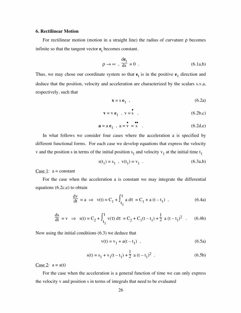
6. Rectilinear Motion
For rectilinear motion (motion in a straight line) the radius of curvature ρ becomes
infinite so that the tangent vector et becomes constant.
ρ → ∞ , detds = 0 . (6.1a,b)
Thus, we may chose our coordinate system so that et is in the positive e1 direction and
deduce that the position, velocity and acceleration are characterized by the scalars s,v,a,
respectively, such that
x = s e1 , (6.2a)
v = v e1 , v = •s , (6.2b,c)
a = a e1 , a = •v = ••s . (6.2d,e)
In what follows we consider four cases where the acceleration a is specified by
different functional forms. For each case we develop equations that express the velocity
v and the position s in terms of the initial position s1 and velocity v1 at the initial time t1
s(t1) = s1 , v(t1) = v1 . (6.3a,b)
Case 1: a = constant
For the case when the acceleration a is constant we may integrate the differential
equations (6.2c,e) to obtain
dvdt = a ⇒ v(t) = C1 + ∫ t
t1 a dτ = C1 + a (t – t1) , (6.4a)
dsdt = v ⇒ s(t) = C2 + ∫ t
t1 v(τ) dτ = C2 + C1(t – t1) +
12 a (t – t1)2 . (6.4b)
Now using the initial conditions (6.3) we deduce that
v(t) = v1 + a(t – t1) , (6.5a)
s(t) = s1 + v1(t – t1) + 12 a (t – t1)2 . (6.5b)
Case 2: a = a(t)
For the case when the acceleration is a general function of time we can only express
the velocity v and position s in terms of integrals that need to be evaluated

27
v(t) = v1 + ∫ tt1
a(τ) dτ , (6.6a)
s(t) = s1 + ∫ tt1
v(τ) dτ . (6.6b)
Case 3: a = a(v)
The case when the acceleration is a function of velocity occurs often when damping
or air drag are modeled. For this case the differential equation (6.2e) yields
dvdt = a(v) ⇒
dva(v) = dt . (6.7a,b)
Thus, with the help of the initial condition (6.3b) we may obtain an equation for v(t) of
the form
∫v(t)v1
dV
a(V) = ∫ tt1
dτ = (t – t1) . (6.8)
Then s(t) can be determined by the solution (6.6b).
Alternatively, sometimes it is of interest to find v(s) directly. For this case v is
thought of as a function of s and the chain rule of differentiation is used to deduce that
a(v) = ddt [v(s(t))] =
dv(s)ds •s = v
dv(s)ds . (6.9)
Thus, the velocity v(s) can be determined by evaluating the integral
∫v(s)v1
VdVa(V) = ∫ s
s1 dS = (s – s1) . (6.10)
Finally, using (6.10) the differential equation (6.2c) yields
dsdt = v(s) ⇒
dsv(s) = dt , (6.11a,b)
which may be integrated to obtain an equation for s(t) of the form
∫s(t)s1
dS
v(S) = ∫ tt1
dτ = (t – t1) . (6.12)
Case 4: a = a(s)
The case when the acceleration is a function of position occurs often when springs are
modeled. For this case we may multiply the differential equation (6.2e) by •s =v to obtain

28
•s dvdt = v
dvdt = a(s) •s , (6.13)
which may be integrated using the initial conditions (6.3) to obtain
∫v(s)v1
V dV = 12 [v(s)2 – v1
2] = ∫ ss1
a(S) dS . (6.14)
Thus, v(s) becomes
v(s) = ± [v12 + 2 ∫ s
s1 a(S) dS ]1/2
. (6.15)
Then, using (6.12) it is possible to determine s(t).

29
7. Polar Coordinates
By way of introduction to the description of general planar motion in terms of polar
coordinates let us first consider circular planar motion. For this case the position vector
may be expressed in the form
x = x1 e1 + x2 e2 , (7.1)
where the rectangular Cartesian coordinates x1,x2 may be expressed in terms of the radius
r of the circle and the angle θ by (see Fig. 7.1)
x1 = r cosθ , x2 = r sinθ . (7.2a,b)
e1
e2 e
r
e!
!
Fig. 7.1
Thus, the position vector may be expressed in the form
x = r (cosθ e1 + sinθ e2) = r er , (7.3)
where er is the unit vector in the direction of the point of interest
er = er(θ) = cosθ e1 + sinθ e2 , er • er = 1 . (7.4a,b)
Furthermore, we define the unit vector eθ by
eθ(θ) = derdθ = – sinθ e1 + cosθ e2 , eθ • eθ = 1 , (7.5a,b)
which points in the direction of increasing θ (see Fig. 7.1). Also, note that er and eθ are
orthogonal vectors
er • eθ = 0 , (7.6)

30
and that the derivative of eθ with respect to θ is related to er by the expression
deθdθ = – er . (7.7)
It follows from (5.2) and the above definitions that for constant radius r the increment
of arclength ds is related to the angle increment dθ by
(ds)2 = dx • dx = dxdθ •
dxdθ (dθ)2 = (r eθ) • (r eθ) (dθ)2 , (7.8a)
(ds)2 = r2 (dθ)2 , ds = r dθ . (7.8b,c)
Furthermore, recall from (5.3) that the tangent vector is given by
et = dxds =
dxdθ
dθds = (r eθ)
1r = eθ . (7.9)
Thus, for circular motion eθ is tangent to the path. Also, using (5.5) we may determine
that the normal vector en and the radius of curvature ρ are given by
detds =
deθdθ
dθds = –
1r er =
1ρ en , (7.10a)
ρ = r , en = – er . (7.10b,c)
For general planar motion the position vector is a function of time parametrically
through the polar coordinates {r,θ} and may be expressed in terms of the polar base
vectors er and eθ by
x = x(t) = r er(θ) , r = r(t) , θ = θ(t) . (7.11a,b,c)
It is important to emphasize that unlike for rectangular Cartesian coordinates the position
vector in polar coordinates is not equal to the sum of the coordinates times their
associated base vectors. This is because the base vectors er and eθ are functions of the
angular coordinate θ, so that er already is directed towards the point of interest. Now,
differentiation of (7.1a) yields
v = •x = •r er + r •er . (7.12)
Using the definition (7.5a) we may deduce that

31
•er = derdθ
•θ =
•θ eθ , (7.13)
so the velocity becomes
v = •r er + r •θ eθ = vr er + vθ eθ . (7.14)
Recalling from (5.14a) that the velocity is always tangent to the particle path the tangent
vector et may be determined by the equation
et = v|v| =
vr er + vθ eθ(vr
2 + vθ2)1/2 . (7.15)
This shows that for the general planar case eθ is not tangent to the path of motion. Next,
differentiation of (7.14) yields the acceleration in the form
a = •v = ••r er + •r •er + •r •θ eθ + r
••θ eθ + + r
•θ •eθ , (7.16a)
= ••r er + •r •θ eθ + •r
•θ eθ + r
••θ eθ – r
•θ2 er , (7.16b)
= [••r – r •θ2] er + [r
••θ + 2 •r
•θ] eθ , (7.16c)
= [••r – r •θ2] er +
1r
d(r2•θ)
dt eθ = ar er + aθ eθ , (7.16d)
The physical interpretation of the velocity components in (7.14) and the acceleration
components in (7.16c) may be summarized as follows
•r er velocity due to changing length of the position vector
r •θ eθ velocity due to changing direction of the position vector
••r er acceleration due to changing radial velocity
– r •θ2 Centripetal acceleration: acceleration due to changing eθ direction
r ••θ eθ acceleration due to changing angular speed
•θ
2 •r •θ eθ Corriolis acceleration due to motion in a rotating coordinate system
32
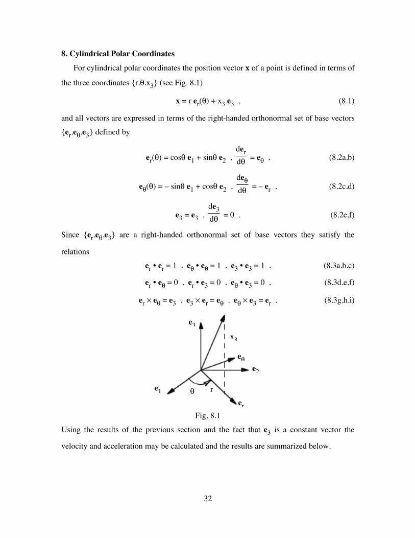
8. Cylindrical Polar Coordinates
For cylindrical polar coordinates the position vector x of a point is defined in terms of
the three coordinates {r,θ,x3} (see Fig. 8.1)
x = r er(θ) + x3 e3 , (8.1)
and all vectors are expressed in terms of the right-handed orthonormal set of base vectors
{er,eθ,e3} defined by
er(θ) = cosθ e1 + sinθ e2 , derdθ = eθ , (8.2a,b)
eθ(θ) = – sinθ e1 + cosθ e2 , deθdθ = – er , (8.2c,d)
e3 = e3 , de3dθ = 0 . (8.2e,f)
Since {er,eθ,e3} are a right-handed orthonormal set of base vectors they satisfy the
relations
er • er = 1 , eθ • eθ = 1 , e3 • e3 = 1 , (8.3a,b,c)
er • eθ = 0 , er • e3 = 0 , eθ • e3 = 0 , (8.3d,e,f)
er × eθ = e3 , e3 × er = eθ , eθ × e3 = er . (8.3g,h,i)
Fig. 8.1
Using the results of the previous section and the fact that e3 is a constant vector the
velocity and acceleration may be calculated and the results are summarized below.
e1
e2
e3
er
eθ
θ r
x3

33
Summary of Cylindrical Polar Coordinates
coordinates r, θ, x3
base vectors er, eθ, e3
derivatives of base vectors derdθ = eθ ,
deθdθ = – er
position vector x = r er(θ) + x3 e3
velocity v = •r er + r •θ eθ + •x3 e3
acceleration [••r – r •θ2] er +
1r
d(r2•θ)
dt eθ + ••x3 e3

34
9. Relative Motion
e1
e2
•
H
s(t)
2e '
1e '
! (t)
BA
•O
Fig. 9.1
By way of introduction to the topic of relative motion consider the example shown in
Fig. 9.1 of a cylinder rolling on a flat surface with point A moving in a slot that rotates
with the cylinder. It is quite difficult to describe the motion of point A relative to the
fixed origin O directly by writing the position vector x(t) relative to e1 and e2. However,
it is possible to describe this complicated motion by separating the description into
smaller simpler parts. In separating the description of motion it is often convenient to use
moving and rotating coordinate axes. It is important to emphasize that depending on how
we separate the motion we can either simplify or complicate the kinematic description.
Since this separation is not unique we will have to develop experience solving many
problems in order to learn the advantages and disadvantages of different separations of
motion.
With reference to Fig. 9.2 we can describe the general motion of point A in terms of
its position x, velocity v, and acceleration a, relative to the fixed origin O by separating
the motion into the sum of the motion of point B, with position vector X and the motion
of A relative to B, with the position vector p. Thus, we have
x = X + p , x = xA , X = xB , (9.1a,b,c)
v = •X + •p , v = vA , •X = vB , (9.1d,e,f)
a = ••X + ••p , a = aA , ••X = aB . (9.1g,h,i)

35
In (9.1) the subscripts A or B are used to denote quantities characterizing the motion of
the points A and B. Also, the position vector p, velocity •p , and acceleration ••p, describe
the relative motion of point A relative to point B. Sometimes it is convenient to express
these vectors in alternative forms that emphasize their relative nature
p = xA/B = xA – xB , (9.2a)
•p = vA/B = vA – vB , (9.2b)
••p = aA/B = aA – aB , (9.2c)
where the notation xA/B denotes the position of A relative to B.
ABSOLUTE AND RELATIVE MOTION
Motion relative to a fixed point in space is called absolute motion whereas motion
relative to a moving point is called relative motion. Thus, with reference to Fig. 9.2, the
quantities xA, vA, aA are called the absolute position, velocity, and acceleration,
respectively, and the quantities xA/B, vA/B, aA/B are called the relative position, velocity,
and acceleration, respectively.
Fig. 9.2
e1
e2
e3
x
O
B
A
e2'
e3'
X=xB
p=xA/B
e1'

36
10. Rotating Coordinate Axes and Angular Velocity
In the description of relative motion it is often convenient to use a rotating coordinate
system like the one shown in Fig. 9.1. Here and throughout the text we let ei be a fixed
right-handed orthonormal set of coordinate axes and let ei' be another right-handed
orthonormal set of coordinate axes that is allowed to rotate in space. By way of
introduction let us first consider the simple case where ei' rotates about a fixed axis e3' ,
which for convenience is identified with e3 (see Fig. 10.1). Thus we take
e1' = cosθ e1 + sinθ e2 , (10.1a)
e2' = – sinθ e1 + cosθ e2 , (10.1b)
e3' = e3 . (10.1c)
e1
e2
2e '
1e '
!(t)
Fig. 10.1
Since ei are fixed their derivatives vanish (•ei =0) so differentiation of (10.1) yields
•e1' = •θ (– sinθ e1 + cosθ e2) =
•θ e2' , (10.2a)
•e2' = •θ (– cosθ e1 – sinθ e2) = –
•θ e1' , (10.2b)
•e3' = 0 . (10.2c)
Now from Fig. 10.1 we observe that the angle θ characterizes the rotation of the ei' axes
about the fixed e3' axis so that •θ characterizes the angular velocity. In this regard it is
important to emphasize that the origin of the rotating coordinate axes ei' can move without

37
changing the description (10.2). Furthermore, by introducing the angular velocity vector
ω defined by
ω = •θ e3' , (10.3)
we can conveniently rewrite equations (10.2) in the compact form
•ei' = ω × ei' , (10.4)
which explicitly states that ω is the angular velocity of the ei' coordinate axes.
In the above we have proved equation (10.4) for the special case of rotation about a
fixed axis in space. However, it can be shown that (10.4) holds even if the angular
velocity ω(t) is a function of times whose magnitude and direction change. To prove this
we recall that since ei' form an orthonormal set of axes they satisfy the conditions
ei' • ej' = δij . (10.5)
In view of the fact that (10.5) is symmetric in the indices (i,j) these equations represent
six constraints on the nine scalar quantities that characterize the three vectors ei'. Thus,
the coordinate axes ei' have only three degrees of freedom, which corespond to three
independent rotations. To show that (10.4) is consistent with the constraints (10.5) we
differentiate (10.5) to obtain
•ei' • ej' + ei' • •ej' = 0 . (10.6)
Next, substitution of (10.4) into (10.6) yields
•ei' • ej' + ei' • •ej' = (ω × ei') • ej' + ei' • (ω × ej') = ω • (ei' × ej') + (ej' × ei') • ω ,
= ω • [ei' × ej' + ej' × ei'] = 0 . (10.7)
This means that the differential equations (10.4) satisfy the differential form (10.6) of the
constraint (10.5) so that the vectors ei' calculated by integrating (10.4) for arbitrary ω will
remain an orthonormal set of vectors. Thus, the components ωi' = ω • ei' of the angular
velocity ω represent the rates of rotation of the rotating coordinate axes about the each of
the axes ei', respectively. Finally, we represent ω in terms of its magnitude ω and
direction eω

38
ω = ω eω , eω • eω = 1 , (10.8a,b)
and note that the sign convention is chosen so that positive values of ω indicate counter-
clockwise rotation about the positive eω axes.
As an example we can reconsider the cylindrical polar coordinate axes shown in Fig.
10.2 and take
e1' = er , e2' = eθ , e3' = e3 . (10.9a,b,c)
Noting that the angular velocity ω is given by
ω = •θ e3 , (10.10)
the derivatives of the vectors er,eθ,e3 may be calculated using the formula (10.4) to obtain
•er = ω × er = •θ eθ , (10.11a)
•eθ = ω × eθ = – •θ er , (10.11b)
•e3 = ω × e3 = 0 . (10.11c)
e1
e2
e3
er
e!
!•!
!
Fig. 10.2

39
11. General Differential Operator
Returning to our discussion of relative motion we note that vectors can be referred to
any complete set of base vectors. Thus, with reference to Fig. 9.2 the vector p, which
describes the position of point A relative to point B, may be represented in terms of the
base vectors ei' and its components pi' relative to ei' such that
p = pi' ei' . (11.1)
Since in dynamics we are interested in the time rate of change of vectors it is important to
emphasize that whenever we introduce a set of base vectors like ei' we must also define
the angular velocity ω with which the base vectors are rotating. To emphasize this we
write
•ei' = ω × ei' , (11.2)
which explicitly indicates that ω is the angular velocity of the base vectors ei'. This is
particularly important when we use more than one set of rotating base vectors so that
more than one angular velocity is used.
Now, differentiation of (11.1) and use of (11.2) yields
•p = •pi' ei' + pi' •ei' , (11.3a)
•p = •pi' ei' + ω × (pi' ei') . (11.3b)
Thus, the derivative of p naturally separates into two parts
•p = δpδt + ω × p , (11.4)
where the operator δ( )/δt is defined as the frame derivative by
δpδt = •pi' ei' . (11.5)
The physical interpretation of these terms may be explained as follows:

40
δpδt = •pi' ei'
The frame derivative of p is the rate of change of the
vector p measured relative to ei' assuming that ei' do not
rotate.
ω × p The rate of change of the vector p due to the rotation of
the coordinate axes ei'.
The differential operator (11.4) is sometimes called the general operator because it is
valid even if the coordinate system is rotating. It is important to emphasize that the
angular velocity ω that appears in (11.4) characterizes the rate of rotation of the same
coordinate system in which p is represented. For example, if we were to consider a
second coordinate system with base vectors ei'' which rotate with angular velocity Ω
•ei'' = Ω × ei'' , (11.6)
Then the general operator (11.4) would take the form
•p = δpδt + Ω × p ,
δpδt = •pi'' ei'' . (11.7a,b)
Recalling that the vector product ω × p may be calculated using the determinant
ω × p = ⎪⎪⎪
⎪⎪⎪e1' e2' e3'
ω1' ω2' ω3'p1' p2' p3'
, (11.8)
it is very convenient to calculate the derivative of a vector referred to a rotating
coordinate system by writing the following table.

41
e1'
e2'
e3'
ω
ω1'
ω2'
ω3'
p
p1'
p2'
p3'
δpδt
•p1'
•p2'
•p3'
ω × p
ω2' p3' – ω3' p2'
– ω1' p3' + ω3' p1'
ω1' p2' – ω2' p1'
•p
•p1'
+ ω2' p3' – ω3' p2'
•p2'
– ω1' p3' + ω3' p1'
•p3'
+ ω1' p2' – ω2' p1'
Using the general operator (11.4) we can calculate the derivative of any vector. For
example we can calculate the relative acceleration ••p in the form
••p = δ
•pδt + ω × •p , (11.9a)
••p = δδt [
δpδt + ω × p] + ω × [δp
δt + ω × p] , (11.9b)
••p = δ2pδt2 +
δωδt × p + 2 ω ×
δpδt + ω × (ω × p) . (11.9c)
However, using the general operator (11.4) the angular acceleration •ω is given by
•ω =
δωδt + ω × ω =
δωδt , (11.10)
so the relative acceleration (11.9c) becomes
••p = δ2pδt2 + •
ω × p + 2 ω × δpδt + ω × (ω × p) . (11.11)

42
The physical interpretation of these terms may be explained as follows:
δ2pδt2
The acceleration as measured relative to ei' assuming that ei' do not rotate.
•ω × p The acceleration due to the angular acceleration •
ω of the coordinate axes ei'.
2 ω × δpδt
The Corriolis acceleration
ω × (ω × p)
The Centripetal acceleration

43
12. Spherical Polar Coordinates
For spherical polar coordinates the position vector x of a point is defined in terms of
the three coordinates {R,θ,φ} (see Fig. 12.1)
x = R eR(θ,φ) , (12.1)
and all vectors are expressed in terms of the right-handed orthonormal set of base vectors
{eR,eθ,eφ} defined in terms of the cylindrical polar base vectors {er,eθ,e3}by
eR(θ,φ) = cosφ er + sinφ e3 , (12.2a)
eθ(θ) = – sinθ e1 + cosθ e2 , (12.2b)
eφ(θ,φ) = – sinφ er + cosφ e3 , (12.2c)
Since {eR,eθ,eφ} are a right-handed orthonormal set of base vectors they satisfy the
relations
eR • eR = 1 , eθ • eθ = 1 , eφ • eφ = 1 , (12.3a,b,c)
eR • eθ = 0 , eR • eφ = 0 , eθ • eφ = 0 , (12.3d,e,f)
eR × eθ = eφ , eφ × eR = eθ , eθ × eφ = eR . (12.3g,h,i)
In order to calculate derivatives of vectors expressed in spherical coordinates it is
necessary to calculate derivatives of the base vectors. This can be done directly by
deriving the formulas
∂eR∂θ = cosφ eθ ,
∂eR∂φ = eφ , (12.4a,b)
∂eθ∂θ = – cosφ eR + sinφ eφ ,
∂eθ∂φ = 0 , (12.4c,d)
∂eφ∂θ = – sinφ eθ ,
∂eφ∂φ = – eR , (12.4e,f)
and using the chain rule of differentiation. Alternatively we may take
e1' = eR , e2' = eθ , e3' = eφ , (12.5a,b,c)
and write the angular velocity ω in the form (see Fig. 12.1)
ω = •θ e3 – •φ eθ . (12.6)

44
e1
e2
e3
er
e!
!•!
!
e"
"
ReR
"•!
Fig. 12.1
Notice that in (12.6) •θ represents the angular velocity about the e3 axis and •
φ represents
the angular velocity about the (–eθ) axis. Furthermore, using (12.2) we can express the
vector e3 in terms of the spherical base vectors such that
e3 = sinφ eR + cosφ eφ , (12.7)
so the angular velocity ω becomes
ω = •θ sinφ eR – •φ eθ +
•θ cosφ eφ . (12.8)
Now the rate of change of the base vectors may be calculated by
•eR = ω × eR = •θ cosφ eθ + •φ eφ , (12.9a)
•eθ = ω × eθ = – •θ cosφ eR +
•θ sinφ eφ , (12.9b)
•eφ = ω × eφ = – •φ eR – •θ sinφ eθ . (12.9c)
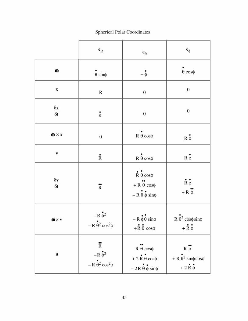
Using the procedure described in the last section we can calculate the velocity and
acceleration in spherical coordinates and the results are summarized in the following
table.
45
Spherical Polar Coordinates
eR
eθ
eφ
ω
•θ sinφ
– •φ
•θ cosφ
x
R
0
0
δxδt
•R
0
0
ω × x
0
R •θ cosφ
R •φ
v
•R
R •θ cosφ
R •φ
δvδt
••R
•R
•θ cosφ
+ R ••θ cosφ
– R •θ •φ sinφ
•R •φ
+ R ••φ
ω × v
– R •φ2
– R •θ2 cos2φ
– R •φ •θ sinφ
+ •R •θ cosφ
R •θ2 cosφ sinφ
+ •R •φ
a
••R
– R •φ2
– R •θ2 cos2φ
R ••θ cosφ
+ 2 •R •θ cosφ
– 2 R •θ •φ sinφ
R ••φ
+ R •θ2 sinφ cosφ
+ 2 •R •φ

46
13. General Rigid Body Motion
Fig. 13.1
A body is said to be rigid if the distance between any two points remains constant.
Letting A and B be two points on the rigid body (see Fig. 13.1) we have
| xA/B |2 = xA/B • xA/B = constant . (13.1)
It follows that the angle θ between any two material lines on the rigid body remains
constant (see Fig. 13.2) so that we can attach a coordinate system ei' to the body that will
remain orthonormal. This coordinate system is called a body coordinate system. Since
the coordinate system ei' is attached to the body its angular velocity ω
•ei' = ω × ei' , (13.2)
is the same as the angular velocity of the rigid body. Now with reference to Fig. 13.1 it is
apparent that a rigid body has 6 degrees of freedom: 3 translational degrees of freedom
characterized by xB ; and 3 rotational degrees of freedom characterized by ω.
The relative velocity between two points A and B on a rigid body may be determined
by referring the relative position vector to the body coordinate system
xA/B = p = pi' ei' . (13.3)
O
e1
e2
e3 e1'
e3'
X = xB
p = xA/B A
B x ω
e2'

47
A
•
•
B
•C!
Fig. 13.2
Then, use of the general operator (11.4) and the expression (13.2) we have
vA/B = •p = δpδt + ω × p . (13.4)
However, since A and B lie on the rigid body and ei' is a body coordinate system the
coordinates pi' are constant so that δp/δt vanishes
δpδt =
δxA/Bδt = •pi' ei' = 0 , (13.5)
and (13.4) reduces to
vA/B = ω × xA/B . (13.6)
Note that this means that the relative velocity vA/B is perpendicular to the relative
position vector xA/B so that
vA/B • xA/B = 0 . (13.7)
Also, note that the result (13.7) is consistent with the basic definition of a rigid body
because it can be obtained by differentiating (13.1).
Furthermore, it follows from (13.6) that the velocity of a general point A may be
expressed in the form
vA = vB + ω × xA/B . (13.8)
Then, the acceleration of point A can be determined by differentiating (13.8) and using
(13.6) to obtain
48
aA = aB + •ω × xA/B + ω × (ω × xA/B) . (13.9)
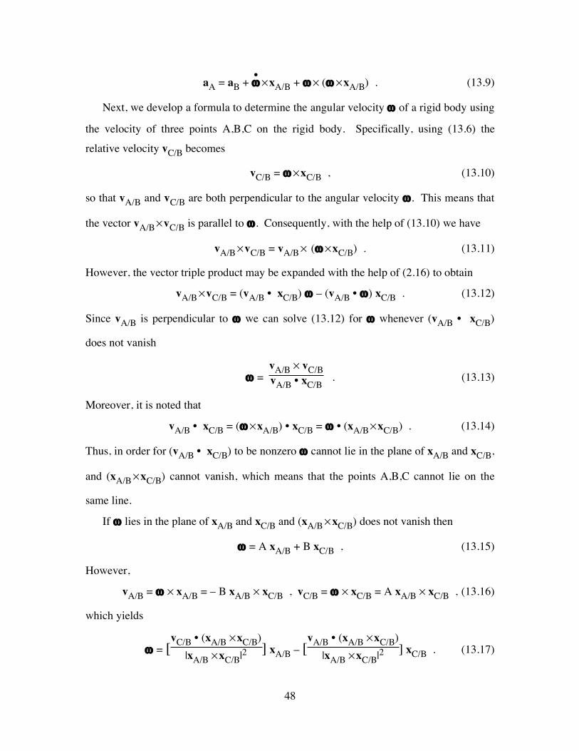
Next, we develop a formula to determine the angular velocity ω of a rigid body using
the velocity of three points A,B,C on the rigid body. Specifically, using (13.6) the
relative velocity vC/B becomes
vC/B = ω × xC/B , (13.10)
so that vA/B and vC/B are both perpendicular to the angular velocity ω. This means that
the vector vA/B × vC/B is parallel to ω. Consequently, with the help of (13.10) we have
vA/B × vC/B = vA/B × (ω × xC/B) . (13.11)
However, the vector triple product may be expanded with the help of (2.16) to obtain
vA/B × vC/B = (vA/B • xC/B) ω – (vA/B • ω) xC/B . (13.12)
Since vA/B is perpendicular to ω we can solve (13.12) for ω whenever (vA/B • xC/B)
does not vanish
ω = vA/B × vC/BvA/B • xC/B
. (13.13)
Moreover, it is noted that
vA/B • xC/B = (ω × xA/B) • xC/B = ω • (xA/B × xC/B) . (13.14)
Thus, in order for (vA/B • xC/B) to be nonzero ω cannot lie in the plane of xA/B and xC/B,
and (xA/B × xC/B) cannot vanish, which means that the points A,B,C cannot lie on the
same line.
If ω lies in the plane of xA/B and xC/B and (xA/B × xC/B) does not vanish then
ω = A xA/B + B xC/B , (13.15)
However,
vA/B = ω × xA/B = – B xA/B × xC/B , vC/B = ω × xC/B = A xA/B × xC/B , (13.16)
which yields
ω = [vC/B • (xA/B × xC/B)
|xA/B × xC/B|2 ] xA/B – [vA/B • (xA/B × xC/B)
|xA/B × xC/B|2 ] xC/B . (13.17)
49
A
B
•
•
!n
L
eA/B
Fig. 13.3
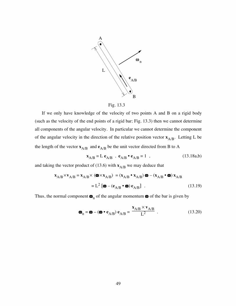
If we only have knowledge of the velocity of two points A and B on a rigid body
(such as the velocity of the end points of a rigid bar; Fig. 13.3) then we cannot determine
all components of the angular velocity. In particular we cannot determine the component
of the angular velocity in the direction of the relative position vector xA/B. Letting L be
the length of the vector xA/B and eA/B be the unit vector directed from B to A
xA/B = L eA/B , eA/B • eA/B = 1 , (13.18a,b)
and taking the vector product of (13.6) with xA/B we may deduce that
xA/B × vA/B = xA/B × (ω × xA/B) = (xA/B • xA/B) ω – (xA/B • ω) xA/B
= L2 [ω – (eA/B • ω) eA/B] . (13.19)
Thus, the normal component ωn of the angular momentum ω of the bar is given by
ωn = ω – (ω • eA/B) eA/B = xA/B × vA/B
L2 . (13.20)

50
14. Instantaneous Screw Motion Of A Rigid Body
Fig. 14.1
In this section we show that the general motion of a rigid body can be described by
the motion of a screw with the rigid body rotating about an axis in space and translating
parallel to this axis. This screw motion is considered to be instantaneous in the sense that
the axis of rotation and velocity of translation can change with time.
For convenience we express the angular velocity ω of the rigid body in terms of its
magnitude ω and direction eω by
ω = ω eω , eω • eω = 1 , (14.1a,b)
and recall from (13.8) that the velocity of a general point A on a rigid body may be
expressed in terms of the velocity vB of another point on the rigid body by the formula
vA = vB+ ω × xA/B . (14.2)
Taking the inner product of (14.2) with the vector eω we may deduce that
vA • eω = vB • eω . (14.3)
O
e1
e2
e3
xA
A
B
C
xA/B
xB
xC/B s ω
axis of rotation
D
51
This means that all points have the same component of velocity in the eω direction. In
other words, the body is advancing in the eω direction with uniform velocity.
Furthermore, since vA is not necessarily parallel to eω we realize that the body is also
rotating about some axis parallel to eω. To find this axis of rotation, let xC locate an
arbitrary point on this axis of rotation and note from (14.3) that all points on this axis
have the same absolute velocity which is parallel to eω so that
vC = (vB • eω) eω . (14.4)
However, since all points C are attached to the same rigid body we may write
vC = vB + ω × xC/B . (14.5)
Using the fact that ω is parallel to vC it follows that
0 = ω × vC = ω × vB + ω × (ω × xC/B)
0 = ω × vB + (ω • xC/B) ω – (ω • ω) xC/B , (14.6)
so that the relative position vector xC/B may be written in the form
xC/B = ω × vBω2 +
(ω • xC/B) ωω2 , (14.7a)
xC/B = xD/B + s eω , xD/B = ω × vBω2 , s = xC/D • eω . (14.7b,c,d)
Notice that the vector xD/B is perpendicular to eω so it locates the point D on the axis of
rotation that is closest to the point B (see Fig. 14.1). Also, the scalar s in (14.7c)
determines the location of an arbitrary point on the axis of rotation as measured from the
point D.
In summary, the rigid body is instantaneously rotating with angular velocity ω about
the axis DC at the same time that it is advancing in the direction eω with uniform velocity
(vB • eω) so the motion can be described as motion of a screw.
For the simpler case of planar motion in the e1–e2 plane the angular velocity ω is in
the constant e3 direction
ω = ω e3 , (14.8)

52
the velocity vB is in the e1–e2 plane so the velocity vC of points on the axis of rotation
vanishes. Thus, the intersection of the axis of rotation with the x3=0 plane is the
instantaneous center of rotation and is given by (14.7b) with s=0
xC/B = ω × vBω2 =
| vB |ω
e3 × vB| e3 × vB |
. (14.9)
The formula (14.9) indicates that the instantaneous center of rotation is located along a
line perpendicular to the velocity vB and a distance |vB| / |ω | from point B (see Fig. 14.2).
It is important to note that ω in (14.8) can be positive or negative so the sign of ω
controls the direction of xC/B in (14.9). Furthermore, since vC vanishes the velocity of an
arbitrary point B on the rigid body is perpendicular to the relative position vector xB/C
because
vB = vC + ω × xB/C = ω × xB/C . (14.10)
Fig. 14.2
e1
e2
C
B
axis of rotation
vB
|vB||ω |
xC/B
ω = ω e3

53
15. Contact of Bodies
Fig. 15.1
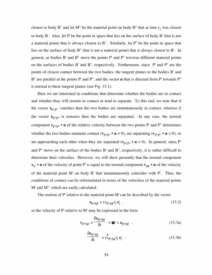
In this section we study the conditions that describe contact and sliding of two bodies.
To this end, consider two bodies B' and B'' that are both translating and rotating in space.
Let ei' be a body coordinate system attached to B' which rotates with angular velocity ω '
so that
•ei' = ω ' × ei' . (15.1)
In what follows it is necessary to distinguish between the locations and velocities of
various points. For example, let M' be the material point on body B' that at time t1 was
Body B'
Body B''
M' P'
P'' M''
ω '
ω ''
Body B'
Body B''
M'
P'
P''
M''
ω '
ω ''
Time t = t1
Time t > t1
n
xP'/M'
xP''/M''
54
closest to body B'' and let M'' be the material point on body B'' that at time t1 was closest
to body B'. Also, let P' be the point in space that lies on the surface of body B' (but is not
a material point) that is always closest to B''. Similarly, let P'' be the point in space that
lies on the surface of body B'' (but is not a material point) that is always closest to B'. In
general, as bodies B' and B'' move the points P' and P'' traverse different material points
on the surfaces of bodies B' and B'', respectively. Furthermore, since P' and P'' are the
points of closest contact between the two bodies, the tangent planes to the bodies B' and
B'' are parallel at the points P' and P'', and the vector n that is directed from P' towards P''
is normal to these tangent planes (see Fig. 15.1).
Here we are interested in conditions that determine whether the bodies are in contact
and whether they will remain in contact or tend to separate. To this end, we note that if
the vector xP'/P'' vanishes then the two bodies are instantaneously in contact, whereas if
the vector xP'/P'' is nonzero then the bodies are separated. In any case, the normal
component vP'/P'' • n of the relative velocity between the two points P' and P'' determines
whether the two bodies maintain contact (vP'/P'' • n = 0), are separating (vP'/P'' • n < 0), or
are approaching each other when they are separated (vP'/P'' • n > 0). In general, since P'
and P'' move on the surface of the bodies B' and B'', respectively, it is rather difficult to
determine their velocities. However, we will show presently that the normal component
vP' • n of the velocity of point P' is equal to the normal component vM' • n of the velocity
of the material point M' on body B' that instantaneously coincides with P'. Thus, the
conditions of contact can be reformulated in terms of the velocities of the material points
M' and M'', which are easily calculated.
The motion of P' relative to the material point M' can be described by the vector
xP'/M' = (xP'/M')i' ei' , (15.2)
so the velocity of P' relative to M' may be expressed in the form
vP'/M' = δxP'/M'δt + ω ' × xP'/M' , (15.3a)
δxP'/M'δt = (•xP'/M')i' ei' . (15.3b)
55
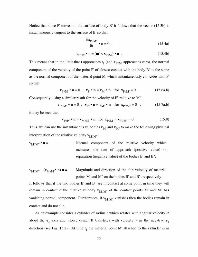
Notice that since P' moves on the surface of body B' it follows that the vector (15.3b) is
instantaneously tangent to the surface of B' so that
δxP'/M'δt • n = 0 , (15.4a)
vP'/M' • n = (ω ' × xP'/M') • n . (15.4b)
This means that in the limit that t approaches t1 (and xP'/M' approaches zero), the normal
component of the velocity of the point P' of closest contact with the body B'' is the same
as the normal component of the material point M' which instantaneously coincides with P'
so that
vP'/M' • n = 0 , vP' • n = vM' • n for xP'/M' = 0 . (15.6a,b)
Consequently, using a similar result for the velocity of P'' relative to M''
vP''/M'' • n = 0 , vP'' • n = vM'' • n for xP''/M'' = 0 . (15.7a,b)
it may be seen that
vP'/P'' • n = vM'/M'' • n for xP'/M' = xP''/M'' = 0 . (15.8)
Thus, we can use the instantaneous velocities vM' and vM'' to make the following physical
interpretation of the relative velocity vM'/M'':
vM'/M'' • n = Normal component of the relative velocity which
measures the rate of approach (positive value) or
separation (negative value) of the bodies B' and B''.
vM'/M'' – (vM'/M''• n) n = Magnitude and direction of the slip velocity of material
points M' and M'' on the bodies B' and B'', respectively.
It follows that if the two bodies B' and B'' are in contact at some point in time they will
remain in contact if the relative velocity vM'/M'' of the contact points M' and M'' has
vanishing normal component. Furthermore, if vM'/M'' vanishes then the bodies remain in
contact and do not slip.
As an example consider a cylinder of radius r which rotates with angular velocity ω
about the e3 axis and whose center B translates with velocity v in the negative e1
direction (see Fig. 15.2). At time t1 the material point M' attached to the cylinder is in

56
contact with a stationary horizontal plane at the material point M''. It follows that the
velocity vM'' vanishes so that the velocity of point M' relative to point M'' is given by
vM'/M'' = vM' = vB + ω × xM'/B = – v e1 + (ω e3) × (– r e2) , (15.9a)
vM'/M'' = (ωr – v) e1 . (15.9b)
Since the relative velocity vM'/M'' has vanishing normal component (vM'/M'' • e2 = 0) the
cylinder remains in contact with the horizontal plane. Furthermore, if ωr > v then point
M' is sliding in the positive e1 direction relative to the fixed point M'' and if ωr < v then
M' is sliding in the negative e1 direction relative to M''. Finally, if ωr = v then the
relative velocity vM'/M'' vanishes and the cylinder rolls without slipping.
•
••
••
•
e1
e2
e2
e1
r
!
M'
M'
P' (t )
P' (t )1
Time t = t1
Time t > t1
v
v
B
B
P' (t )1
M"
M" Fig. 15.2

57
16. Kinetics of a Particle
In the previous sections we have devoted most of our attention to the study of
kinematics of particles and rigid bodies by learning how to analyze position, velocity and
acceleration. Such kinematical quantities are considered to be primitive quantities
because they can be measured directly. In this section we introduce the notion of force
which is a kinetical vector quantity that usually is measured indirectly. In particular, the
magnitude of a force is often measured by comparing it to the weight of an object or by
using the displacement of a spring, which itself has been calibrated by measuring the
weights of standard objects.
Obviously, the direction of a force matters because when we push an object in one
direction it tends to move in that direction, whereas when we push it in the opposite
direction it tends to move in the opposite direction. In fact, for rectilinear motion it can
be shown that the acceleration is in the same direction as the force. To see if this
observation remains true for more general motions we can consider the motion of a ball
on a smooth (frictionless) horizontal plane that is confined to move in a circle by a string
that is attached to a weight (Fig. 16.1). The first thing that we can observe is that the
acceleration vector rotates and is always pointed towards the center of the circle.
Specifically, the acceleration vector a always points in the same direction as the force
vector F which is applied to the ball by the string. Mathematically this means that F is
parallel to a
F | | a . (16.1)
By keeping the weight constant and changing the radius of the circular path we can
observe that the angular velocity of the ball changes in such a way that it preserves the
magnitude of the acceleration. Furthermore, by using the same ball but taking different
weights we can determine that the magnitude of the force F applied by the string on the
ball (which is equal to the weight applied) always remains proportional to the magnitude
of the acceleration. Thus, for different forces {F1 , F2 , F3 } and associated accelerations
{ a1 , a2 , a3 } we have
| F1 || a1 | =
| F2 || a2 | =
| F3 || a3 | = m , (16.2)

58
where the constant of proportionality m is a property of the ball which is called the mass
of the ball.
Fig. 16.1
NEWTONS LAWS OF MOTION
Sir Issac Newton (1642-1727) was the first to discover the correct laws of motion of
particles which are summarized as the following three laws of motion:
Law I: A particle remains at rest or continues to move in a straight line
with uniform velocity if there is no unbalanced force acting on it.
F = 0 ⇒ v = constant . (16.3)
Law II: The resultant force F acting on a particle is equal to the rate of
change of linear momentum.
F = d(mv)
dt . (16.4)
Law III: The forces of action and reaction between interacting bodies are
equal in magnitude and opposite in direction (Fig. 16.2).
FA/B + FB/A = 0 , FA/B = – FB/A . (16.5a,b)
(FA/B is the force applied by body B on body A)

59
A B
A B
FA/B
FB/A
FA
FB
FB
FA
Fig. 16.2
CONSERVATION OF MASS
For our purposes we will only consider bodies that have constant mass so we may
write the law of conservation of mass in the form
dmdt = •m = 0 . (16.6)
BALANCE OF LINEAR MOMENTUM
Newton's second law of motion is referred to in modern terms as the balance of linear
momentum. In words it states that the rate of change of linear momentum (mv) is equal
to the total external force F applied to the body. In view of the conservation of mass
(16.6) the balance of linear momentum can be written in the form
d(mv)
dt = m dvdt = m a = F . (16.7)
It is important to emphasize that the velocity v and the acceleration a in the balance of
linear momentum must be absolute not relative quantities so they must be measured
relative to a fixed point.
Since the balance of linear momentum is a vector equation it may be expressed with
respect to any convenient set of base vectors. For example, if we consider two sets of
rectangular Cartesian base vectors ei and ei' we may write the following scalar equations
Fi = m ai (ei • F = m ei • a) , (16.8a)
Fi' = m ai' (ei' • F = m ei' • a) . (16.8b)
60
Similarly, if we refer the vectors to the cylindrical polar base vectors {er , eθ , e3} or the
spherical polar base vectors {eR , eθ , eφ} we may write
Fr = m ar , Fθ = m aθ , F3 = m a3 , (16.9)
or
FR = m aR , Fθ = m aθ , Fφ = m aφ . (16.10)
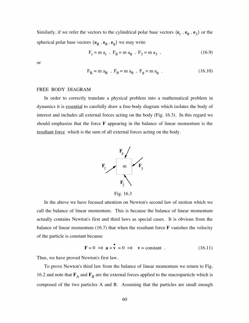
FREE BODY DIAGRAM
In order to correctly translate a physical problem into a mathematical problem in
dynamics it is essential to carefully draw a free-body diagram which isolates the body of
interest and includes all external forces acting on the body (Fig. 16.3). In this regard we
should emphasize that the force F appearing in the balance of linear momentum is the
resultant force which is the sum of all external forces acting on the body.
F1
F2
F3
F4
m
Fig. 16.3
In the above we have focused attention on Newton's second law of motion which we
call the balance of linear momentum. This is because the balance of linear momentum
actually contains Newton's first and third laws as special cases. It is obvious from the
balance of linear momentum (16.7) that when the resultant force F vanishes the velocity
of the particle is constant because
F = 0 ⇒ a = •v = 0 ⇒ v = constant . (16.11)
Thus, we have proved Newton's first law.
To prove Newton's third law from the balance of linear momentum we return to Fig.
16.2 and note that FA and FB are the external forces applied to the macroparticle which is
composed of the two particles A and B. Assuming that the particles are small enough

61
and remain in contact it follows from continuity that they both move with the same
acceleration a
aA = aB = a . (16.12)
Letting mA be the mass of particle A and mB be the mass of particle B, the balance of
linear momentum applied to the macroparticle of total mass mA+ mB yields the equation
FA + FB = (mA+ mB) a . (16.13)
Alternatively, we can consider the free body diagrams of the particles A and B separately
and denote FA/B as the internal force (contact force) applied by particle B on particle A,
and denote FB/A as the internal force applied by particle A on particle B. Then the
balances of linear momentum of each of the particles may be written in the forms
FA + FA/B = mA a , FB + FB/A = mB a . (16.14a,b)
Next, we add equations (16.14a,b) and subtract (16.13) from the result to deduce that
FA/B + FB/A = 0 , (16.15)
which proves Newton's third law. The main theoretical point associated with this proof is
the basic assumption that the conservation of mass and the balance of linear momentum
are valid for any arbitrary part of a body (which in this case includes both the
macroparticle and the two particles, separately).
D'ALEMBERT'S PRINCIPLE
In order to extend the principle of virtual work for static problems to dynamical
problems d'Alembert (1717-1783) introduced the notion of the "force of inertia" I,
defined in terms of the mass of a particle and its absolute acceleration by
I = – m a . (16.16)
Using this definition the balance of linear momentum (16.7) can be rewritten in the form
F + I = 0 . (16.17)
This changes the balance of linear momentum into a principle that states that every body
is in a state of "dynamical equilibrium". In our opinion, the introduction of the concept
of an inertial force confuses the concept of force since acceleration is a kinematical
quantity that can be measured independently of the concept of force and mass is an
intrinsic property of the body that is independent of the particular motion of the body.

62
Furthermore, the introduction of the concept of "dynamical equilibrium" does not
simplify the formulation of the balance of linear momentum because it still requires the
calculation of the absolute acceleration a. Also, since the balance of linear momentum
and the principle of "dynamical equilibrium" (16.17) are mathematically identical, any
mathematical operation performed on equation (16.17) can be performed on equation
(16.7) to obtain the same result.
TWO MAIN PROBLEMS IN DYNAMICS
There are two main problems in the study of dynamics which can be summarized as
follows:
Problem I: Given the motion and mass of a particle, determine the
resultant force necessary to create this motion. This problem is relatively
simple because we just need to differentiate the motion to determine the
absolute acceleration and then use the balance of linear momentum to
determine the resultant force.
Problem II: Given the resultant force acting on a particle and its mass,
determine the motion of the particle. This problem is much more difficult
than problem I because we need to integrate the equations of motion.
Because of the analytical difficulty with integrating the set of nonlinear equations of
motion that usually result in dynamical problems we will focus most of our attention to
either problem I or to the formulation (but not solution) of problem II.

63
17. Vibrations
In this section we consider the physically important problem of both free and forced
vibration of a damped spring-mass system. To this end, let us first consider the simple
problem of free vibrations of the undamped spring-mass system shown in Fig. 17.1. The
spring has a free length L and spring constant k and the body has mass m. Friction is
neglected but gravity is included.
k , L
x(t)
m
e1
e2 g
mg
N
k(x – L)
Fig. 17.1
Recalling that the force in a spring is equal to the spring constant k times the change
in its length relative to its force-free length L, we may use the free body diagram of the
mass m in Fig. 17.1 to write the resultant external force F in the form
F = – k(x – L) e1 + [ N – mg ] e2 , (17.1)
where N is the contact force that the horizontal plate applies to the mass and mg is the
force of gravity. Notice that the origin of the coordinate system has been chosen
conveniently so that x is the current length of the spring and the position of the mass.
Furthermore, since the mass is only allowed to move in the horizontal direction its
acceleration is given by
a = ••x e1 . (17.2)

64
Thus, the balance of linear momentum yields the following vector equation
– k(x – L) e1 + [ N – mg ] e2 = m ••x e1 , (17.3)
which gives the following scalar equations
m ••x + k (x – L) = 0 , N = mg . (17.4a,b)
The first of these equations is a differential equation to determine the position x of the
mass and the second merely states that the contact force is equal to the force of gravity.
Noting that L is constant, equation (17.4a) may be rewritten in the form
d2
dt2 (x – L) + ωn2 (x – L) = 0 , ωn
2 = km , (17.5a,b)
where the constant ωn is called the natural frequency and it has the units of inverse time.
The general solution of (17.5a) may be written in terms of sines and cosines and takes the
form
x – L = A1 sin(ωnt) + A2 cos(ωnt) , (17.6)
where A1 and A2 are constants of integration to be determined by the initial conditions
x(0) = x0 , •x(0) = v0 . (17.7a,b)
However, for ease of interpretation it is more convenient to rewrite (17.6) as
x – L = A [ A1A sin(ωnt) +
A2A cos(ωnt)] , A = (A1
2 + A22 )1/2 , (17.8a,b)
and recall the trigonometric relation
sin(ωnt +φ) = sin(ωnt) cosφ + cos(ωnt) sinφ , (17.9)
to deduce that the general solution of (17.5) may be expressed in the alternative form
x – L = A sin(ωnt + φ) . (17.10)
In (17.10) it is easy to see that A is the amplitude of the vibration and φ is the phase
angle. These constants (A,φ) are determined by the initial conditions (17.7) which yield
the equations
x0 – L = A sinφ , v0 = A ωn cosφ . (17.11a,b)
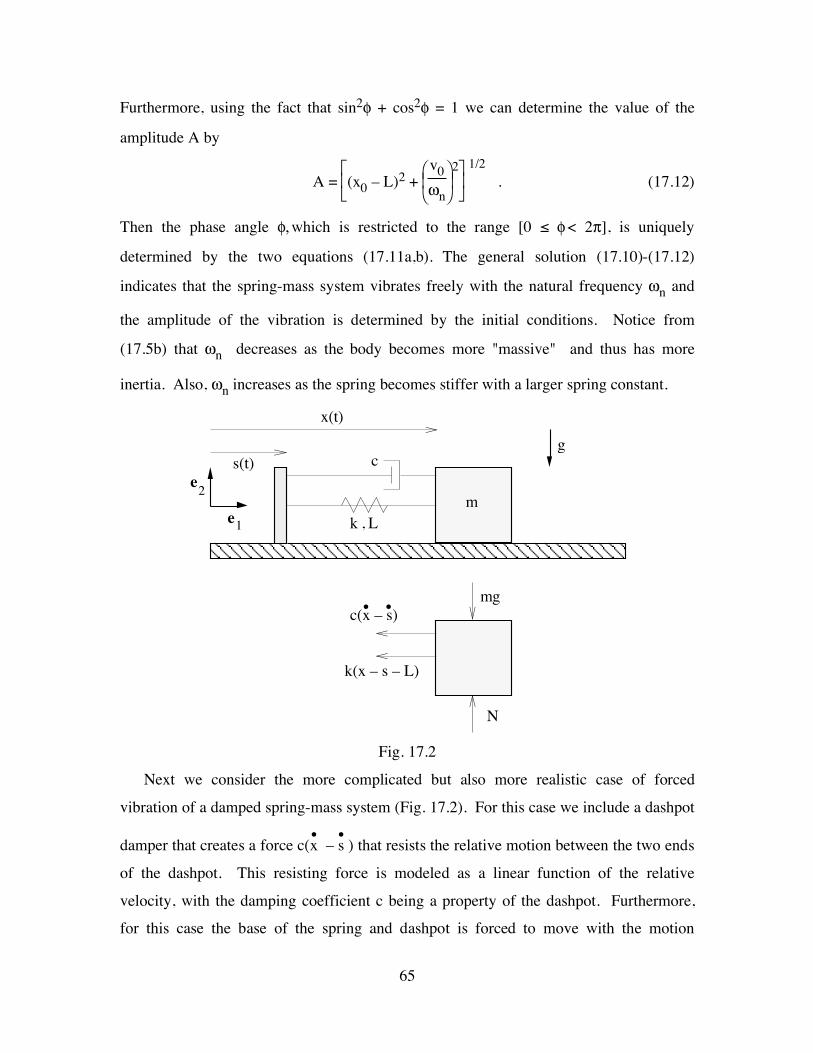
65
Furthermore, using the fact that sin2φ + cos2φ = 1 we can determine the value of the
amplitude A by
A = ⎣⎢⎡
⎦⎥⎤
(x0 – L)2 + ⎝⎜⎛
⎠⎟⎞v0
ωn
2 1/2
. (17.12)
Then the phase angle φ, which is restricted to the range [0 ≤ φ < 2π], is uniquely
determined by the two equations (17.11a,b). The general solution (17.10)-(17.12)
indicates that the spring-mass system vibrates freely with the natural frequency ωn and
the amplitude of the vibration is determined by the initial conditions. Notice from
(17.5b) that ωn decreases as the body becomes more "massive" and thus has more
inertia. Also, ωn increases as the spring becomes stiffer with a larger spring constant.
k , L
x(t)
me
1
e2
g
mg
N
k(x – s – L)
s(t) c
•c(x – s)
•
Fig. 17.2
Next we consider the more complicated but also more realistic case of forced
vibration of a damped spring-mass system (Fig. 17.2). For this case we include a dashpot
damper that creates a force c(•x – •s ) that resists the relative motion between the two ends
of the dashpot. This resisting force is modeled as a linear function of the relative
velocity, with the damping coefficient c being a property of the dashpot. Furthermore,
for this case the base of the spring and dashpot is forced to move with the motion

66
described by s(t). Also, since the current length of the spring is given by (x – s) the
resultant force applied to the mass becomes
F = [ – k(x – s – L) – c(•x – •s) ] e1 + [ N – mg ] e2 . (17.13)
Since x is the position of the mass m measured relative to a fixed wall, the absolute
acceleration of the mass is still given by (17.2) so the vector equation representing the
balance of linear momentum is given by
[ – k(x – s – L) – c(•x – •s) ] e1 + [ N – mg ] e2 = m ••x e1 , (17.14)
and the two scalar equation become
m ••x + k(x – s – L) + c(•x – •s) = 0 , N = mg . (17.15a,b)
By dividing (17.15a) by the mass m and using the definition (17.5b) for the natural
frequency ωn we may rewrite (17.15a) in the form
••w + cm •w + ωn
2 w = – ••s , w = x – s – L , (17.16a,b)
where the quantity w denotes the extension of the spring from its stress-free length L.
Integration of (17.16a) requires the specification of the function s(t) and the initial
conditions (17.7).
In order to understand the influence of damping we first consider the case of free
damped vibrations for which the base is held constant so that s(t) vanishes and the
balance of linear momentum (17.16a) reduces to
••w + cm •w + ωn
2 w = 0 . (17.17)
By using the transformation
w(t) = exp(– ct
2m ) ξ(t) , (17.18)
together with the results
•w = exp(– ct
2m ) [ •ξ –
c2m ξ ] , (17.19a)
••w = exp(– ct
2m ) [ ••ξ –
cm
•ξ + ⎝
⎛⎠⎞c
2m2 ξ ] . (17.19b)
we can transform (17.17) into the simpler form

67
••ξ + ωn
2 (1–ζ2) ξ = 0 , c = 2mζωn , (17.20)
where ζ is a non-dimensional damping parameter. Now, the initial conditions (17.7) with
•s(0) = 0 may be used with the definitions (17.16b) and (17.18) to deduce that
w(0) = x0 – s0 – L , •w(0) = v0 , (17.21a,b)
ξ(0) = x0 – s0 – L , •ξ(0) = v0 + ζωn (x0 – s0 – L) , (17.21c,d)
Noting that (17.20) is similar to (17.5a) we obtain three types of solutions which are
differentiated by the relative value of the damping coefficient ζ.
Underdamped (ζ < 1)
w(t) = exp(– ζωnt) A sin(ω*t + φ) , (17.22a)
ω* = ωn 1–ζ2 , (17.22b)
A = ⎣⎢⎡
⎦⎥⎤
(x0 – s0 – L)2 + ⎩⎨⎧
⎭⎬⎫v0
ω* + ζωnω* (x0 – s0 – L)
2 1/2
, (17.22c)
sinφ = 1A (x0 – s0 – L) , cosφ =
1Aω* [ v0 + ζωn (x0 – s0 – L)] . (17.22d,e)
Critically Damped (ζ = 1)
w(t) = exp(– ωnt) [(x0 – s0 – L) + {v0 + ωn(x0 – s0 – L)} t] , (17.23)
Overdamped (ζ > 1)
w(t) = exp(– ζωnt) A sinh(ω*t + φ) , (17.24a)
ω* = ωn ζ2 – 1 , (17.24b)
A = ⎣⎢⎡
⎦⎥⎤
⎩⎨⎧
⎭⎬⎫v0
ω* + ζωnω* (x0 – s0 – L)
2 – (x0 – s0 – L)2
1/2 , (17.24c)
sinhφ = 1A (x0 – s0 – L) , coshφ =
1Aω* [ v0 + ζωn (x0 – s0 – L)] . (17.24d,e)
In deriving the solution (17.24a) we have followed similar procedures used to derive the
solution (17.10) and have used the hyperbolic identities
sinh(ω*t + φ) = sinh(ω*t) coshφ + cosh(ω*t) sinhφ , (17.25a)

68
cosh2φ – sinh2φ = 1 . (17.25b)
Notice that because of the presence of the exponential terms in (17.22a),(17.23a) and
(17.23a) each of these solutions yields the same equilibrium solution of vanishing w for
long times (large values of t). More specifically, (17.22a) is called an underdamped
solution because it exhibits oscillations that damp to zero; solution (17.23a) is called
critically damped because the damping coefficient ζ attains its critical value (ζ=1, the
minimum value necessary to damp to zero without any oscillation); and solution (17.24a)
is called overdamped because ζ attains a value larger than its critical value. This response
for v0 = 0 is shown in Fig. 17.3 for different values of the damping coefficient ζ.
-1.0
-0.5
0.0
0.5
1.0
!=0.1!=1.0!=2.0
0.0 5.0 10.0 15.0 20.0"
nt
No
rmal
ized
Am
pli
tud
e
Fig. 17.4
The above solution indicates that when damping is present (ζ >0) the homogeneous
solutions of (17.16a) damp out so that after a reasonably long time the only solution that
remains is the particular solution. As a special case let us consider the problem where the
base vibrates with frequency ω and amplitude s0 such that
s(t) = s0 sin(ωt) , (17.26)
so that (17.16a) reduces to
••w + cm •w + ωn
2 w = s0 ω2 sin(ωt) . (17.27)

69
Now, the particular solution wp of (17.27) may be written in the form
wp(t) = A sin(ωt + φ) , (17.28)
where the amplitude A and phase angle φ are to be determined. Substituting (17.28) into
(17.27) we obtain
A [ { }ωn2 – ω2 sin(ωt + φ) + 2ζωnω cos(ωt + φ)] = s0ω
2 sin(ωt) , (17.29a)
A [ (ωn2 – ω2) {sin(ωt) cos(φ) + cos(ωt) sin(φ)}
+ 2ζωnω {cos(ωt) cos(φ) – sin(ωt) sin(φ)}] = s0 ω2 sin(ωt) , (17.29b)
A [ (ωn2 – ω2) {sin(ωt) cos(φ) + cos(ωt) sin(φ)}
+ 2ζωnω {cos(ωt) cos(φ) – sin(ωt) sin(φ)}] = s0 ω2 sin(ωt) , (17.29b)
A[{(ωn
2
ω2 – 1) cos(φ) – 2ζωnω sin(φ)}sin(ωt)
+ {(ωn
2
ω2 – 1) sin(φ) + 2ζωnω cos(φ)}cos(ωt) ] = s0 sin(ωt) . (17.29c)
It follows that the term cos(ωt) can be eliminated by appropriately specifying the phase
angle φ so the solution becomes
A = s0 G(ωn,ζ,ω) , (17.30a)
G(ωn,ζ,ω) = 1
⎣⎢⎡
⎦⎥⎤
⎝⎜⎛
⎠⎟⎞ωn
2
ω2 – 12
+ ⎝⎜⎛
⎠⎟⎞2ζωn
ω
2 1/2 , (17.30b)
sinφ = – 2ζωnω G(ωn,ζ,ω) , cosφ = ⎝
⎜⎛
⎠⎟⎞ωn
2
ω2 – 1 G(ωn,ζ,ω) , (17.30c,d)
where G(ωn,ζ,ω) is called the amplification function because it determines how much the
amplitude A of the response w is amplified relative to the forcing amplitude s0.

70
From a physical point of view we are often more interested in the absolute motion of
the mass instead of its motion relative to the base which is described by w. Thus, using
(17.16b), (17.28) and (17.30) the solution for the position x of the mass becomes
x(t) = L + s0 sin(ωt) + G(ωn,ζ,ω) s0 sin(ωt + φ) . (17.31)
This solution can be written in the simpler form
x(t) = L + s0 g(ωn,ζ,ω) sin(ωt + Φ) , (17.32)
where the amplification function g and the phase angle Φ associated with the absolute
motion of the mass are determined by the equations
g cosΦ = 1 + G cosφ , g sinΦ = G sinφ . (17.33)
Now using the results (17.30b,c,d) we may deduce that
g2 = (1 + G cosφ)2 + (G sinφ)2 = 1 + 2G cosφ + G2 , (17.34a)
g =
⎣⎢⎡
⎦⎥⎤1 + 4ζ2
⎝⎜⎛
⎠⎟⎞ω
ωn
2
⎝⎜⎛
⎠⎟⎞
1 – ω2
ωn2
2
+ 4ζ2⎝⎜⎛
⎠⎟⎞ω
ωn
2
1/2
. (17.34b)
The main physical implications of this solution can be observed by considering the
following limiting cases:
Limit ω << ωn
g ≈ 1 , Φ ≈ 0 , x(t) ≈ L + s(t) , (17.35a)
Limit ω = ωn
g ≈ 12ζ 1+4ζ2 , Φ ≈ – tan-1 (
12ζ), (17.35b)
Limit ω >> ωn
g ≈ 0 , Φ ≈ – π2 , x(t) ≈ L , (17.35c)
This means that for very low forcing frequencies (ω<<ωn) the mass moves with the base;
for very high forcing frequencies (ω>>ωn) the mass is isolated from the base vibration
because it does not move at all. Furthermore, for very low and very high forcing
frequency the limiting solution is independent of the value of damping. In contrast, when
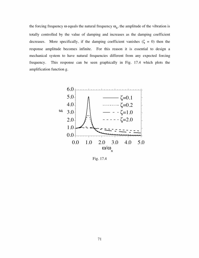
71
the forcing frequency ω equals the natural frequency ωn, the amplitude of the vibration is
totally controlled by the value of damping and increases as the damping coefficient
decreases. More specifically, if the damping coefficient vanishes (ζ = 0) then the
response amplitude becomes infinite. For this reason it is essential to design a
mechanical system to have natural frequencies different from any expected forcing
frequency. This response can be seen graphically in Fig. 17.4 which plots the
amplification function g.
0.0
1.0
2.0
3.0
4.0
5.0
6.0
!=0.1
!=0.2
!=1.0
!=2.0
0.0 1.0 2.0 3.0 4.0 5.0"/"
n
g
Fig. 17.4
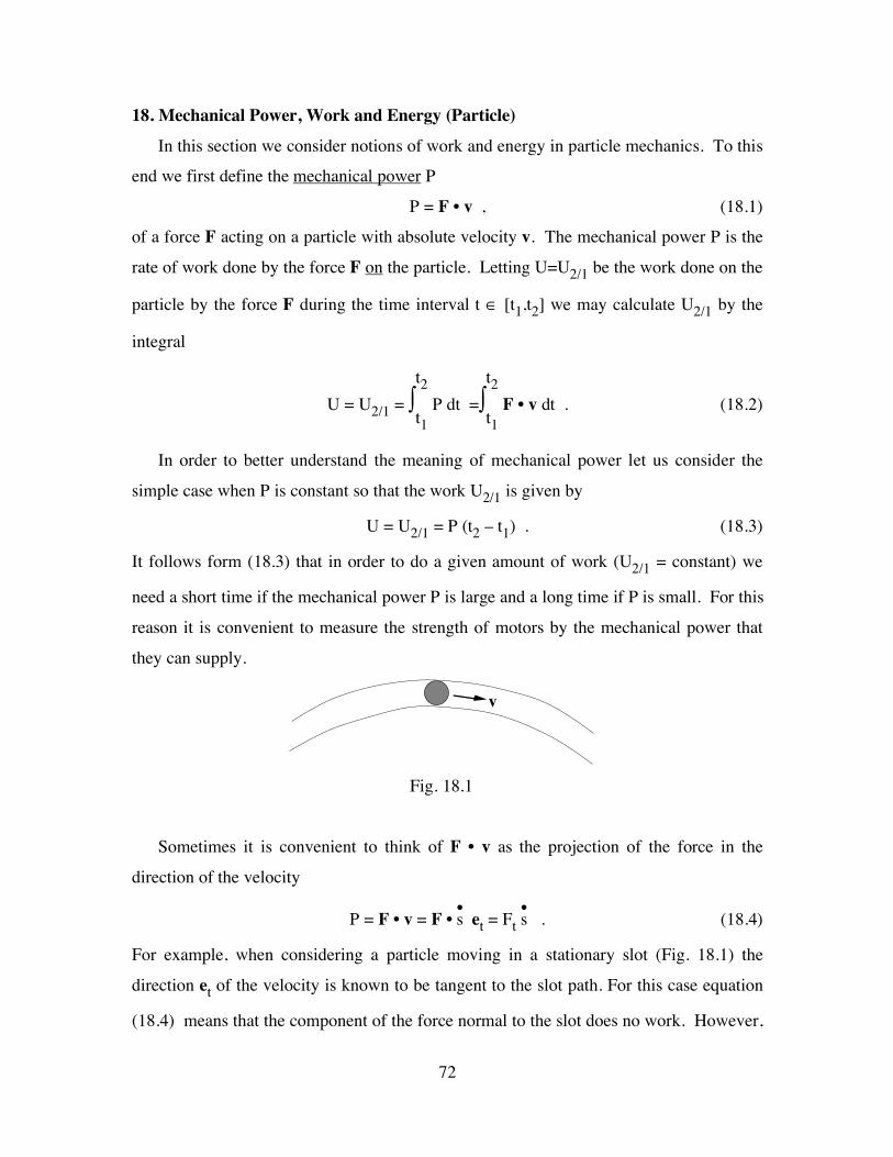
72
18. Mechanical Power, Work and Energy (Particle)
In this section we consider notions of work and energy in particle mechanics. To this
end we first define the mechanical power P
P = F • v , (18.1)
of a force F acting on a particle with absolute velocity v. The mechanical power P is the
rate of work done by the force F on the particle. Letting U=U2/1 be the work done on the
particle by the force F during the time interval t ∈ [t1,t2] we may calculate U2/1 by the
integral
U = U2/1 = ∫t2 t1
P dt =∫t2 t1
F • v dt . (18.2)
In order to better understand the meaning of mechanical power let us consider the
simple case when P is constant so that the work U2/1 is given by
U = U2/1 = P (t2 – t1) . (18.3)
It follows form (18.3) that in order to do a given amount of work (U2/1 = constant) we
need a short time if the mechanical power P is large and a long time if P is small. For this
reason it is convenient to measure the strength of motors by the mechanical power that
they can supply.
v
Fig. 18.1
Sometimes it is convenient to think of F • v as the projection of the force in the
direction of the velocity
P = F • v = F • •s et = Ft •s . (18.4)
For example, when considering a particle moving in a stationary slot (Fig. 18.1) the
direction et of the velocity is known to be tangent to the slot path. For this case equation
(18.4) means that the component of the force normal to the slot does no work. However,

73
when the slot is not stationary then (18.4) still holds but et is no longer tangent to the path
of the slot so the component of the force normal to the slot does work on the particle. R
eR
mM
F
Fig. 18.2
Sometimes it is convenient to think of F • v as the projection of the velocity in the
direction of the force. For example, when considering the force of gravity acting between
two particles of masses M and m (Fig. 18.2) the direction of the force F is known
P = F • v = FR (eR • v) . (18.4)
If the force F is the total resultant force applied to a particle of mass m then the
balance of linear momentum (16.7) may be used to rewrite the mechanical power in the
form
P = F • v = m a • v = ddt ⎝
⎛⎠⎞1
2 m v • v = •T, (18.5)
where the kinetic energy T is defined by
T = 12 m v • v =
12 m v2 . (18.6)
Now, substitution of (18.5) into (18.2) yields
U = U2/1 =∫t2 t1
•T dt = T2 – T1 , (18.7)
which states that the work done by the resultant force applied to a particle is equal to the
change in kinetic energy of the particle. In order to emphasize that U in (18.7) is the
work done by the resultant force let us consider the example of a motor lifting a mass m
from position 1 to position 2 in a gravitational field (Fig. 18.3). Assuming that at the
beginning and end of the process the mass is at rest it follows that the kinetic energies T1
and T2 vanish so that the work U also vanishes. In order to explain how the work U can
vanish when we lift a weight we note that the resultant force F is composed of the force

74
due to gravity and the force due to the motor. Since the work done by F vanishes we may
conclude that work done by the motor (which is positive) exactly balances the work done
by gravity (which is negative).
mPosition 2:
Position 1:
g
Fig. 18.3
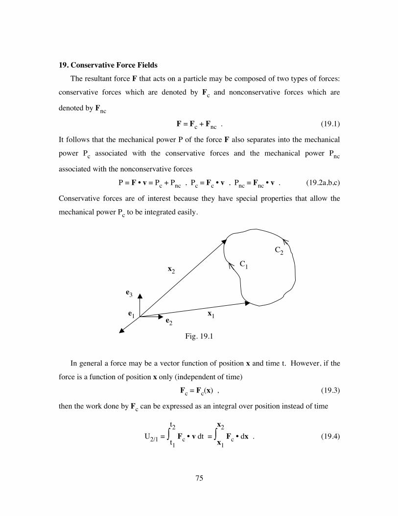
75
19. Conservative Force Fields
The resultant force F that acts on a particle may be composed of two types of forces:
conservative forces which are denoted by Fc and nonconservative forces which are
denoted by Fnc
F = Fc + Fnc . (19.1)
It follows that the mechanical power P of the force F also separates into the mechanical
power Pc associated with the conservative forces and the mechanical power Pnc
associated with the nonconservative forces
P = F • v = Pc + Pnc , Pc = Fc • v , Pnc = Fnc • v . (19.2a,b,c)
Conservative forces are of interest because they have special properties that allow the
mechanical power Pc to be integrated easily.
Fig. 19.1
In general a force may be a vector function of position x and time t. However, if the
force is a function of position x only (independent of time)
Fc = Fc(x) , (19.3)
then the work done by Fc can be expressed as an integral over position instead of time
U2/1 = ∫t2 t1
Fc • v dt = ∫x2 x1
Fc • dx . (19.4)
e1 e2
e3
x2
x1
C1
C2
76
For a general function Fc the work done traversing path C1 from x1 to x2 is different from
that traversing path C2 (see Fig. 19.1). However, if the work done by Fc is path
independent
∫x2 C1:x1
Fc • dx = ∫x2 C2:x1
Fc • dx , (19.5)
then Fc is called a conservative force field. It follows from (19.5) that the work done by
a conservative force Fc depends only on the end points of integration so the integral over
an arbitrary closed path vanishes
∫O Fc • dx = 0 . (19.6)
It can be shown that Fc is a conservative force field with (19.6) holding for any
closed path if and only if there exists a potential V(x) which is a function of position only
such that
Fc = – ∇ V = – ∂V∂x , Fci = –
∂V∂xi
, (19.7a,b)
where Fci and xi are the components of Fc and x, relative to the fixed Cartesian base
vectors ei. Now, substitution of (19.7) into (19.4) yields
U2/1 = ∫x2 x1
Fc • dx = ∫x2 x1
[– ∂V∂x • dx] = ∫
x2 x1
[– dV]
U2/1 = – [ V(x2) – V(x1) ] = – (V2 – V1) . (19.8)
This means that the work done on the particle by a conservative force equals minus the
change in potential energy.
Notice from (19.7a) that since a potential function exists for a conservative force Fc
the conservative force field satisfied the vector equation
∇ × Fc = ∇ × (– ∇ V) = 0 . (19.9)
It follows that if ∇ × Fc = 0 and Fc is independent of time then Fc is a conservative force
field and a potential V(x) exists that is independent of time which is related to Fc by

77
equation (19.7a). These conditions can be used to check if a given force field is
conservative or not. Tables 19.1 and 19.2 summarize useful vector formulas in
cylindrical polar coordinates and spherical polar coordinates, respectively.
Notice from (19.2b) and (19.7a) that the mechanical power of a conservative force is
equal to minus the rate of change of the potential
Pc = Fc • v = – ∂V∂x • •x = –
•V , (19.10)
because the potential V is independent of time. In order to understand why a
conservative force field must be independent of time we note that if a force field Fnc(x,t)
is a function of position and time and yet satisfies the equation
∇ × Fnc(x,t) = 0 , (19.11)
then a potential function Vnc(x,t) of position and time exits such that
Fnc(x,t) = – ∇ Vnc(x,t) = – ∂Vnc∂x . (19.12)
However, for this case the mechanical power Pnc associated with Fnc is not equal to the
total derivative of the potential because
Pnc = Fnc • v = – ∂Vnc∂x • •x = –
•Vnc +
∂Vnc∂t . (19.13)
This means that Fnc is not a conservative force field because the work done traversing a
given path depends on the speed at which the path is traversed.
In the following we consider examples of four common conservative force fields and
one common nonconservative field.
CONSTANT FORCE FIELD
Let Fc = b where b is a constant vector. Since Fc is independent of time and
independent of space it satisfies equation (19.9) so we know that Fc is a conservative
force field. The functional form for the potential V is obtained by integrating
Fc = – ∇ V , ∂V∂xi
= – Fci = – bi , (19.14a,b)
to obtain
V = V0 – bi xi = V0 – b • x , (19.15)
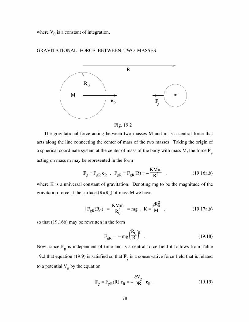
78
where V0 is a constant of integration.
GRAVITATIONAL FORCE BETWEEN TWO MASSES
eR
R
M m
R0
Fg
Fig. 19.2
The gravitational force acting between two masses M and m is a central force that
acts along the line connecting the center of mass of the two masses. Taking the origin of
a spherical coordinate system at the center of mass of the body with mass M, the force Fg
acting on mass m may be represented in the form
Fg = FgR eR , FgR = FgR(R) = – KMm
R2 , (19.16a,b)
where K is a universal constant of gravitation. Denoting mg to be the magnitude of the
gravitation force at the surface (R=R0) of mass M we have
| FgR(R0) | = KMm
R02 = mg , K =
gR02
M , (19.17a,b)
so that (19.16b) may be rewritten in the form
FgR = – mg ⎝⎜⎛
⎠⎟⎞R0
R2 . (19.18)
Now, since Fg is independent of time and is a central force field it follows from Table
19.2 that equation (19.9) is satisfied so that Fg is a conservative force field that is related
to a potential Vg by the equation
Fg = FgR(R) eR = – ∂Vg∂R eR . (19.19)

79
Using (19.18) we have
Vg = V∞ – ∫R ∞
FgR(ξ) dξ = V∞ + ∫R ∞
mgR0
2
ξ2 dξ , (19.20a)
Vg = V∞ – mgR0
2
R , (19.20b)
where V∞ is the value of the gravitational potential Vg at R=∞. It follows that the change
in potential energy is given by
Vg2 – Vg1 = mgR02 ⎝⎜⎛
⎠⎟⎞1
R1 –
1R2
> 0 for R2 > R1 . (19.21)
This means that the gravitational potential increases as the distance between the masses
increases.
GRAVITATION CLOSE TO THE EARTH
m
R = R + x0 3
x3
eRe
3=
Fig. 19.3
For the gravitational force field close to the surface of the earth the height x3 above the
surface of the earth is quite small relative to the radius R0 of the earth so that the position
R of the mass m may be approximated by
R = R0 + x3 = R0 ⎝⎜⎛
⎠⎟⎞
1 + x3R0
, (19.22a)
1R =
1
R0 ⎝⎜⎛
⎠⎟⎞
1 + x3R0
≈ 1
R0 ⎝⎜⎛
⎠⎟⎞
1 – x3R0
, (19.22b)
so that the gravitational potential (19.20b) may be approximated by

80
Vg = V∞ – mgR0 ⎝⎜⎛
⎠⎟⎞
1 – x3R0
= (V∞ – mgR0) + mg x3 , (19.23a)
Vg = V0 + mg x3 , V0 = V∞ – mgR0 , (19.23b,c)
where V0 is the value of the gravitational potential at the surface of the earth. Notice
again that the gravitational potential increases as the distance between the mass m and the
surface of the earth increases (x3 increases). At the surface of the earth the force of
gravity g per unit mass (often called the acceleration of gravity) is approximately 9.81
m/s2.
ELASTIC POTENTIAL OF A SPRING
m
eR
•
R
meF
Fig. 19.4
Consider a spring whose free length is L and whose elastic force acting on the mass m is
given by
Fe = FeR(R) eR . (19.24)
Since Fe is independent of time and is a central force field it is a conservative force field
with the potential Ve given by
Ve = – ∫R L
FeR(ξ) dξ , (19.25)
where we have taken Ve = 0 when the spring is force free with R=L. For a linear spring
we have

81
FeR = – k(R – L) , Ve = 12 k (R – L)2 . (19.26a,b)
NONCONSERVATIVE FORCE FIELD
k , L
x(t)
m
e1
e2 g
mg
N
k(x – L)
µ
Ff
Fig. 19.5
An important example of a nonconservative force field is the force Ff due to sliding
friction. Consider the mass m sliding on a flat plane with friction coefficient µ shown in
Fig. 19.4. Since the force of friction always opposes the motion of the mass we may
express Ff in terms of the velocity v of the mass by the equation
Ff = – µ N v
| v | for v ≠ 0 , (19.27)
where N is the magnitude of the normal force applied by the plane on the mass. In order
to show that the friction force Ff is nonconservative we calculate the mechanical power
Pf due to Ff
Pf = Ff • v = – µ N v • v | v | < 0 for v ≠ 0 . (19.28)
Thus the rate of work done by friction on the mass is always negative so energy is always
dissipated and the force of friction is nonconservative.

82
Table 19.1: Cylindrical Polar Coordinates
x = r er(θ) + x3 e3
F = Fr er + Fθ eθ + F3 e3
∇ V = ∂V∂r er +
1r ∂V∂θ eθ +
∂V∂x3
e3
∇ • F = 1r ∂(rFr)∂r +
1r ∂Fθ∂θ +
∂F3∂x3
∇ × F = ⎣⎢⎡
⎦⎥⎤1
r ∂F3∂θ –
∂Fθ∂x3
er + ⎣⎢⎡
⎦⎥⎤∂Fr
∂x3 – ∂F3∂r eθ + ⎣
⎢⎡
⎦⎥⎤1
r ∂(rFθ)∂r –
1r ∂Fr∂θ e3
∇2 V = ∂2V∂r2 +
1r ∂V∂r +
1r2 ∂2V∂θ2 +
∂2V∂x3
2
Table 19.2: Spherical Polar Coordinates
x = R eR(θ,φ)
F = FR eR + Fθ eθ + Fφ eφ
∇ V = ∂V∂R eR +
1R cosφ
∂V∂θ eθ +
1R ∂V∂φ eφ
∇ • F = 1
R2 ∂(R2FR)∂R +
1R cosφ
∂Fθ∂θ +
1R cosφ
∂(Fφ cosφ)∂φ
∇ × F = 1
R cosφ ⎣⎢⎡
⎦⎥⎤∂Fφ
∂θ – ∂(Fθ cosφ)
∂φ eR + 1R ⎣⎢⎡
⎦⎥⎤∂FR
∂φ – ∂(RFφ)∂R eθ
+ 1
R cosφ ⎣⎢⎡
⎦⎥⎤∂(RFθ cosφ)
∂R – ∂FR∂θ eφ
∇2 V = 1
R2 ∂∂R ⎝
⎛⎠⎞R2 ∂V
∂R + 1
R2 cos2φ ∂2V∂θ2 +
1R2 cosφ
∂∂φ ⎝⎜
⎛⎠⎟⎞cosφ
∂V∂φ

83
20. Energy Equation For A Particle
With the help of (18.2) and (18.7) it follows that we can write an energy equation for
a particle in the form
U2/1 = ∫t2 t1
F • v dt = (T2 – T1) , (20.1)
where T1 and T2 are values of the kinetic energy T at the times t1 and t2, respectively,
and U2/1 is the work done by all forces acting on the particle. In view of the simple
relationship (19.10) between the mechanical power and the time rate of change of the
potential associated with a conservative force field it is convenient to separate the total
force F into known conservative force fields Fg associated with gravity, Fe associated
with elastic springs, and the remainder –F such that
F = Fg + Fe + –F , F • v = – •Vg –
•Ve + –F • v , (20.2a,b)
where Vg is the gravitational potential given by (19.20b) or (19.23.b), and Ve is the
elastic potential given by (19.26b). Defining the work –U 2/1 done by the force –F
–U2/1 = ∫t2 t1
–F • v dt , (20.3)
we may rewrite (10.1) in the convenient form
–U2/1 = (T2 – T1) + (Vg2 – Vg1) + (Ve2 – Ve1) = (E2 – E1) , (20.4)
where the total energy E is equal to the sum of the kinetic energy and the potential
energies which are not included in the work done by –F
E = T + Vg + Ve . (20.5)
Equation (20.5) states that the work done by –F on the particle is equal to the change in
total energy E. In particular, notice that if all forces acting on the particle are
conservative then –U2/1 vanishes and the total energy E remains constant.

84
When –U2/1 vanishes or the mechanical power –F • v is a simple expression which can
be integrated with respect to time, the energy equation (20.4) can be a very convenient
equation to use in obtaining the solution of a particular problem. However, we must
emphasize that the energy equation (20.4) is merely a scalar integral of the vectorial
equations of motion (16.7) and therefore it does not include additional information about
the motion of a particle. In this sense the energy equation may be used to replace one of
the three scalar equations associated with the balance of linear momentum (16.7) but we
must remember that by itself, the energy equation can only provide a single piece of
information about the motion of the particle.

85
21. Linear And Angular Momentum Of A Particle
BALANCE OF LINEAR MOMENTUM
For a single particle it is sometimes convenient to introduce a definition of the linear
momentum G of the particle
G = m v , (21.1)
and rewrite the balance of linear momentum (16.7) in the form
•G = F . (21.2)
In words equation (21.2) states that the rate of change of linear momentum is equal to the
total force acting on the particle. It should be recalled that the velocity v that appears in
the definition (21.1) is the absolute velocity which is measured relative to a fixed point in
space.
BALANCE OF ANGULAR MOMENTUM THEOREM
Although the balance of linear momentum (21.2) characterizes the complete motion
of a particle it is sometimes desirable to introduce the notion of the angular momentum
Ho of the particle relative to the fixed origin O of a coordinate system by the expression
Ho = x × G , (21.3)
where x(t) is the position of the particle relative to the point O. Now differentiating
(21.3) with respect to time and using (21.1) and (21.2) we may deduce that
•Ho = •x × G + x × •G = v × m v + x × F = x × F , (21.4)
which means that
•Ho = Mo , (21.5)
where Mo is the moment of the force F applied about the fixed point O
Mo = x × F . (21.6)
In words, the balance of angular momentum (21.5) states that the rate of change of
angular momentum about a fixed point is equal to the resultant moment about the same
fixed point. It is important to emphasize that for a single particle the balance of angular
momentum (21.5) is a theorem which has been proved using the balance of linear
momentum. In this sense, the balance of angular momentum does not introduce new
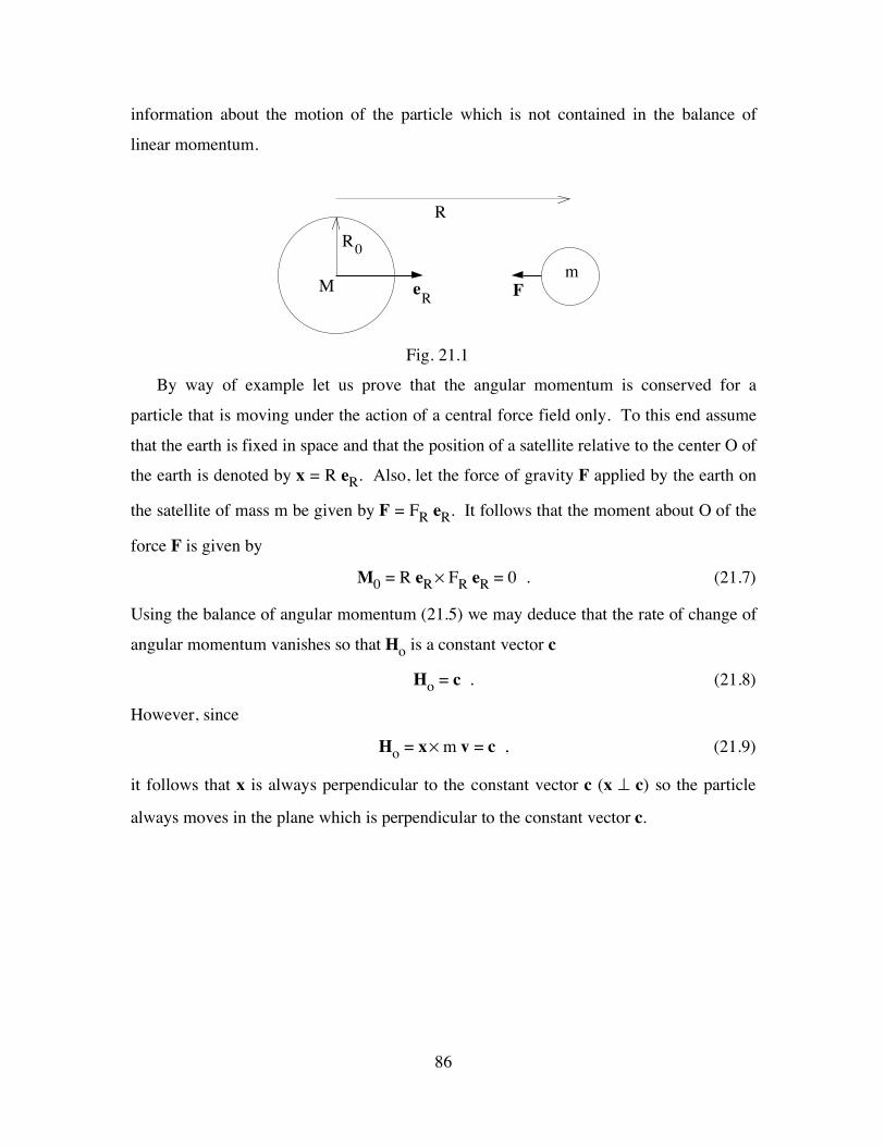
86
information about the motion of the particle which is not contained in the balance of
linear momentum.
eR
R
Mm
F
R0
Fig. 21.1
By way of example let us prove that the angular momentum is conserved for a
particle that is moving under the action of a central force field only. To this end assume
that the earth is fixed in space and that the position of a satellite relative to the center O of
the earth is denoted by x = R eR. Also, let the force of gravity F applied by the earth on
the satellite of mass m be given by F = FR eR. It follows that the moment about O of the
force F is given by
M0 = R eR × FR eR = 0 . (21.7)
Using the balance of angular momentum (21.5) we may deduce that the rate of change of
angular momentum vanishes so that Ho is a constant vector c
Ho = c . (21.8)
However, since
Ho = x × m v = c , (21.9)
it follows that x is always perpendicular to the constant vector c (x ⊥ c) so the particle
always moves in the plane which is perpendicular to the constant vector c.

87
22. Conservation Of Momentum (?)
Sometimes it is easy to observe that one or more components of linear momentum G
or angular momentum Ho are conserved (remain constant). When this happens part of
the equations of motion of a particle integrate simply so it is convenient to use the
integrated equations instead of the differential equations. For example, it follows from
the balances of linear momentum (21.2) and angular momentum (21.5) that both linear
and angular momentum are conserved if the force F vanishes
F = 0 ⇒ G = constant , (22.1a)
F = 0 ⇒ Mo = 0 ⇒ Ho = constant . (22.1b)
In view of the simplicity of the equations (22.1a,b) it is reasonable to consider what
might happen if only one component of force or moment vanish. In particular, let us
consider the case where the component of the force F in the b direction vanishes. It
follows from (21.2) that
b • F = 0 ⇒ •G • b = 0 . (22.2)
The question then arises as to what can be said about the component of linear momentum
in the same direction b that the force component vanishes. To answer this question let us
differentiate the component b • G to obtain
d(b • G)
dt = ––––––•b • G = •b • G + b • •G = •b • G . (22.3)
Equation (22.3) shows that in general the component of linear momentum G in the
direction b is not constant (conserved) even though the component of force F in the same
direction vanishes. However, if the direction b is constant so that •b vanishes then the
component of linear momentum in the direction b will be conserved. This means that a
component of linear or angular momentum is conserved whenever a component of force
or moment vanishes in a fixed direction b.
By way of example let us consider the motion of a particle of mass m which moves
under the action of a force F which in cylindrical polar coordinates is expressed in the
form
F = Fr er . (22.4)

88
From the point of view of linear momentum it follows from (22.4) that
eθ • •G = 0 , e3 • •G = 0 . (22.5a,b)
Since eθ is not a constant vector we do not expect the component eθ • G to be constant
whereas we do expect the component e3 • G to be constant. More specifically, we have
x = r er + x3 e3 , v = •r er + r •θ eθ + •x3 e3 , (22.6a,b)
G = m ( •r er + r •θ eθ + •x3 e3 ) , (22.6c)
•G = m [ (••r – r •θ2) er + (2 •r
•θ + r
••θ) eθ + ••x3 e3 ] , (22.6d)
Using (22.5) it follows that
eθ • •G = 0 ⇒ 2 •r •θ + r
••θ = 0 ⇒
1r
ddt (r2
•θ) = 0 , (22.7a)
e3 • •G = 0 ⇒ ••x3 = 0 ⇒ ddt (
•x3) = 0 . (22.7b)
Consequently,
r2 •θ = constant , •x3 = constant . (22.8a,b)
This means that eθ • G = mr•θ is not necessarily constant whereas e3 • G = m•x3 is
constant. However, the result (22.8a) indicates that something is conserved.
To determine the physical meaning of (22.8a) let us consider the balance of angular
momentum. It follows from (22.4) that
Mo = x × F = (r er + x3 e3) × Fr er = x3 Fr eθ . (22.9)
Thus there is no moment the er and e3 directions so we expect the component of angular
momentum in the e3 direction to be preserved. To see this consider
Ho = x × m v = (r er + x3 e3) × m ( •r er + r •θ eθ + •x3 e3 ) , (22.10a)
Ho = m [ – r •θx3 er + (•r x3 – r •x3) eθ + (r2
•θ) e3 ] . (22.10b)
Using (22.9) and (22.10b) we have
89
e3 • Mo = 0 ⇒ e3 • Ho = constant ⇒ r2•θ = constant , (22.11)
which shows that the result (22.8b) indicates that angular momentum about the e3 axis is
conserved.

90
23. Impulse And Momentum
In view of the simplicity of the balance of linear momentum (21.2) and the balance of
angular momentum (21.5) it follows that the changes in momentum from time t1 to time
t2 can be determined by integrating these balance laws over time. In particular, it is
convenient to define F̂ as the impulsive force due to F
F̂ = ∫t2 t1
F dt , (23.1)
and use the balance of linear momentum (21.2) to deduce that
F̂ = ∫t2 t1
•G dt = G2 – G1 . (23.2)
This states that the impulsive force is equal to the change in linear momentum.
Similarly, we can define M̂o as the impulsive moment due to Mo
M̂o = ∫t2 t1
Mo dt , (23.3)
and use the balance of angular momentum (21.5) to deduce that
M̂o = ∫t2 t1
•Ho dt = Ho2 – Ho1 . (23.4)
This states that the impulsive moment about a fixed point is equal to the change in
angular momentum about the same fixed point.
By way of example consider the one-dimensional problem of the impact of two
masses mA and mB. Before impact mass mA moves with constant velocity v0 towards
mass mB and mass mB is stationary. After impact we assume that both masses move
together with common velocity v (see Fig. 23.1). Neglecting friction, the only forces
acting on the two masses are gravity, and the contact force between themselves and the
floor. Let FA/B be the force applied by mass mB on mass mA and let FB/A be the force
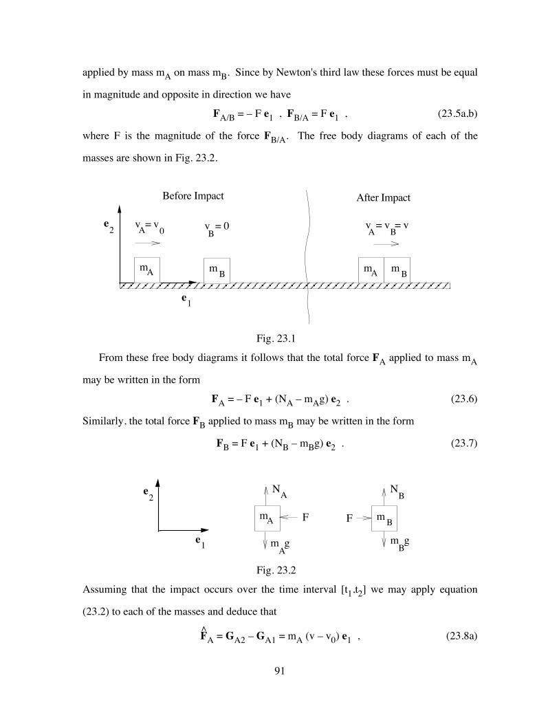
91
applied by mass mA on mass mB. Since by Newton's third law these forces must be equal
in magnitude and opposite in direction we have
FA/B = – F e1 , FB/A = F e1 , (23.5a,b)
where F is the magnitude of the force FB/A. The free body diagrams of each of the
masses are shown in Fig. 23.2.
mA B
m mA B
m
v = vA 0
v = 0B
Before Impact After Impact
v = v = vA B
e1
e2
Fig. 23.1
From these free body diagrams it follows that the total force FA applied to mass mA
may be written in the form
FA = – F e1 + (NA – mAg) e2 . (23.6)
Similarly, the total force FB applied to mass mB may be written in the form
FB = F e1 + (NB – mBg) e2 . (23.7)
mA B
m
e1
e2
F F
NA
m gA
NB
m gB
Fig. 23.2
Assuming that the impact occurs over the time interval [t1,t2] we may apply equation
(23.2) to each of the masses and deduce that
F̂A = GA2 – GA1 = mA (v – v0) e1 , (23.8a)
92
F̂B = GB2 – GB1 = mB v e1 , (23.8b)
Next we consider the determination of the impulsive force F̂A. By definition
F̂A = ∫t2 t1
[ – F e1 + (NA – mAg) e2 ] dt . (23.9)
During the impact the forces NA and mAg remain bounded but the force F may become
quite large. As a simple approximation we can assume that the impact occurs over an
infinitesimally short time so the impulse due to NA and mAg vanish but the impulse due
to F does not so that
F̂A = limitt2→ t1 ∫
t2 t1
[ – F e1 + (NA – mAg) e2 ] dt
= – limitt2→ t1 ∫
t2 t1
F e1 dt = – F̂ e1 . (23.10)
Similarly the impulsive force F̂B becomes
F̂B = limitt2→ t1 ∫
t2 t1
F e1 dt = F̂ e1 . (23.11)
Now, substitution of the results (23.10) and (23.11) into the equations (23.8a,b) we may
deduce that
F̂ = – mA (v – v0) , F̂ = mB v . (23.12a,b)
Solving these equations for v and F̂ we have
v = ⎝⎜⎛
⎠⎟⎞mA
mA + mB v0 , F̂ = ⎝
⎜⎛
⎠⎟⎞mA mB
mA + mB v0 . (23.13a,b)
Notice that if mB is small relative to mA then v → v0 and F̂ → 0, whereas if mB is much
greater than mA then v → 0 and F̂ → mA v0.

93
In the above analysis we have considered the dynamics of each mass separately.
However, sometimes it is of interest to consider the properties of the system of two
masses. To this end, let G be the sum of the linear momentum of each of the masses so
that before impact we have
G = G1 = mA v0 e1 , (23.14)
and after impact we have
G = G2 = (mA v + mB v) e1 = (mA + mB) ⎝⎜⎛
⎠⎟⎞mA
mA + mB v0 e1 = mA v0 e1 . (23.15)
This means that the total linear momentum of the system of two masses did not change
during the impact. We can also consider what happens to the total kinetic energy T,
which is the sum of the kinetic energies of the two masses. Before impact we have
T = T1 = 12 mA v0
2 , (23.16)
whereas after impact we have
T = T2 = 12 mA v2 +
12 mB v2 = ⎝
⎜⎛
⎠⎟⎞mA
mA + mB 12 mA v0
2 , (23.17)
so that kinetic energy is lost during the impact
T2 – T1 = – ⎝⎜⎛
⎠⎟⎞mB
mA + mB 12 mA v0
2 < 0 . (23.18)
In a more complete analysis it could be shown that kinetic energy is converted into heat
during the dissipative process which causes the two masses to stick together after impact.

94
24. Kinetics Of Systems Of Particles
Fig. 24.1
Consider a set of N particles and let a typical particle, called the i'th particle have
mass mi, and position xi, relative to a fixed origin. Furthermore, let Fi be the external
force (external to the system) applied to the i'th particle and let fij be the internal force
applied by the j'th particle on the i'th particle. Then the balance of linear momentum for
the i'th particle may be expressed in the form
•Gi = ddt (mi vi) = Fi + ∑j=1
N fij i=1,2,...,N (no sum on i) . (24.1)
In the above it is assumed that fii vanishes (i.e. the i'th particle does not apply an internal
force on itself). Notice that the N vector equations of motion (24.1) are sufficient to
determine the motion of all the N particles in the system. Sometimes it is convenient to
determine what can be said about the system as a whole. To this end, let us define F to
be the total external force applied to the system, f to be the total internal force, and G to
be the total linear momentum of the system
G = ∑i=1
N Gi , F = ∑
i=1
N Fi , f = ∑i=1
N ∑j=1
N fij . (24.2a,b,c)
It follows by summing the equations (24.1) that we may write
•G = F + f , (24.3)
e2 e1
e3
xj
xi
Fi
fij
fji Fj mj
mi
O

95
which is a single vector equation characterizing the balance of linear momentum of the
system of particles.
A vector equation representing the balance of angular momentum of the system of
particles can be obtained by defining the total moment Mo of external forces about the
fixed point O, the total moment mo of internal forces about O, and the total angular
momentum Ho about O
Ho = ∑i=1
N xi × Gi , (24.4a)
Mo = ∑i=1
N xi × Fi , mo = ∑
i=1
N ∑j=1
N xi × fij , (24.4b,c)
Now, taking the cross product of each of equations (24.1) with the position vector xi and
summing the resulting equations we may deduce that
•Ho = Mo + mo . (24.5)
Before continuing let us reconsider the quantities f and mo. In particular by changing
the indices for the summations we have
f = ∑i=1
N ∑j=1
N fij = ∑
j=1
N ∑i=1
N fji , (24.6a)
mo = ∑i=1
N ∑j=1
N xi × fij = ∑
j=1
N ∑i=1
N xj × fji . (24.6b)
Now, interchanging the order of the summations we may deduce that
f = ∑i=1
N ∑j=1
N fij = ∑
i=1
N ∑j=1
N fji , (24.7a)
mo = ∑i=1
N ∑j=1
N xi × fij = ∑
i=1
N ∑j=1
N xj × fji . (24.7b)
By expressing f and mo as the averages of the two representations in (24.7a,b) we may
write

96
f = 12 ∑
i=1
N ∑j=1
N (fij + fji) , (24.8a)
mo = 12 ∑
i=1
N ∑j=1
N (xi × fij + xj × fji) . (24.8b)
Now, in view of Newton's third law, the force fij applied by the mass mj on the mass mi is
equal in magnitude and opposite in direction to the force fji applied by the mass mi on the
mass mj so that
fij = – fji . (24.9)
Substituting (24.9) into (24.8) we have
f = 0 , mo = 12 ∑
i=1
N ∑j=1
N (xi – xj) × fij . (24.10a,b)
Using the result (24.10a) together with equation (24.3) we obtain the equation
•G = F , (24.11)
which states that the resultant external force applied to the system of particles is equal to
the rate of change of linear momentum of the system. Since equation (24.11) is identical
to the balance of linear momentum (21.2) of a single particle it is sometimes convenient
to think of the system of particles as a single particle with total mass m located at the
center of mass –x, such that
m = ∑i=1
N mi , m –x = ∑
i=1
N mi xi . (24.12a,b)
Notice that the location of the center of mass of the system is defined as the mass-
weighted average of the position of the particles. Furthermore, the linear momentum G
and rate of change of linear momentum •G may be expressed in terms of the velocity –v =
–•x and acceleration –a = –•v of the center of mass of the system
G = ∑i=1
N mi vi = m –v , •G = ∑
i=1
N mi ai = m –a . (24.13a,b)

97
Thus, the balance of linear momentum may be written in the form
•G = ddt (m –v) = m –a = F . (24.14)
Equation (24.14) is sometimes called the Principle of Motion of the Center of Mass. In
words it states that relative to an inertial frame of reference the mass center of a system of
particles moves as though the system were a single particle of mass equal to the total
mass of the system moving under the action of the total external force applied to the
system. It is important to note that (24.14) is only a single vector equation so it can only
provide limited information about the motion of the system of N particles.
Notice that even with the help of Newton's third law (24.9) the internal moment mo
does not necessarily vanish (24.10b). Nevertheless, it is of interest to consider three
cases when the internal moment mo vanishes:
Case I: A simple system of particles with the internal forces fij which are central forces
that act along the line of centers of the masses so that
fij = f(xij) (xi – xj) , xij = (xi – xj) • (xi – xj) , (no sum on i,j) (24.15a,b)
where xij is the square of the distance between the masses mi and mj and the function
f(xij) characterizes the force acting between the masses mi and mj.
Case II: Forces perpendicular to the line of centers of the masses are allowed but the
masses are assumed to be in contact so that for some values of i and j we have
xi = xj . (24.16)
Case III: The trivial case when there are no internal forces
fij = 0 . (24.17)
For each of these cases the internal moment mo vanishes and the balance of angular
momentum of the system of particles (24.5) reduces to
•Ho = Mo , (24.18)
which is identical to the balance of angular momentum (21.5) of a single particle.
However, in contrast with the angular momentum equation for a single particle which
was derived as a theorem, the balance of angular momentum (24.18) contains

98
independent information about the system of particles. For example it gives information
about the rotation of the system of particles about its center of mass.
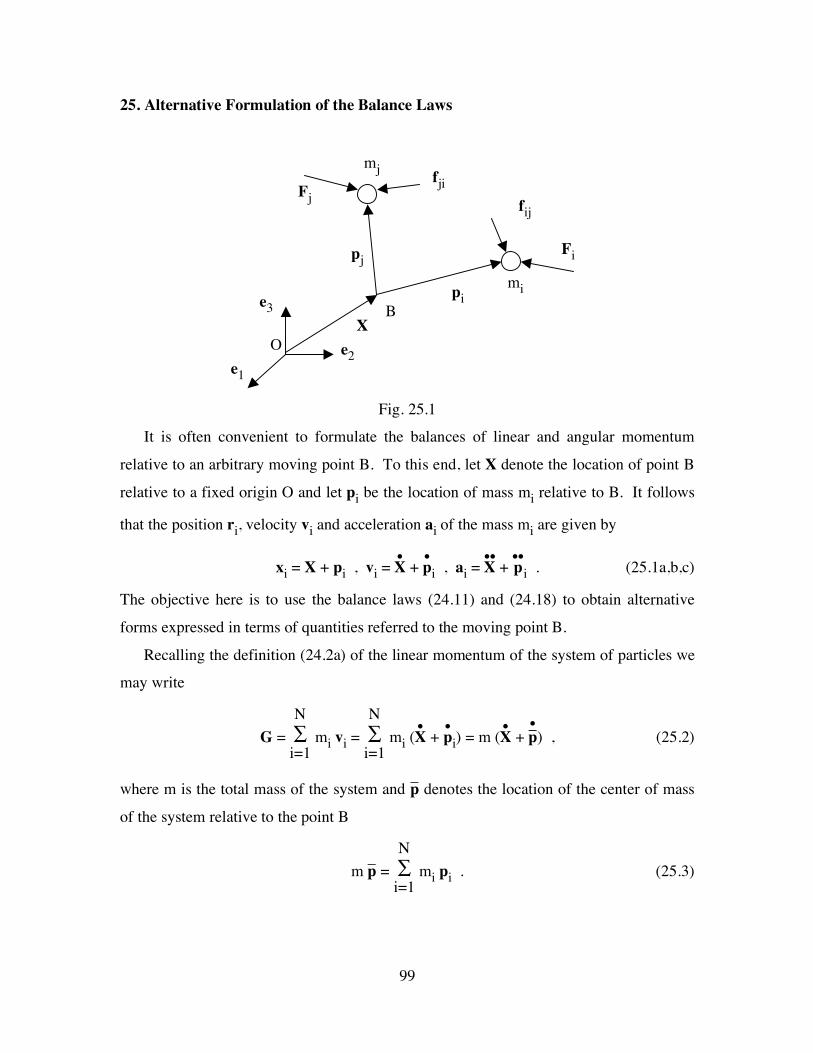
99
25. Alternative Formulation of the Balance Laws
Fig. 25.1
It is often convenient to formulate the balances of linear and angular momentum
relative to an arbitrary moving point B. To this end, let X denote the location of point B
relative to a fixed origin O and let pi be the location of mass mi relative to B. It follows
that the position ri, velocity vi and acceleration ai of the mass mi are given by
xi = X + pi , vi = •X + •pi , ai = ••X + ••pi . (25.1a,b,c)
The objective here is to use the balance laws (24.11) and (24.18) to obtain alternative
forms expressed in terms of quantities referred to the moving point B.
Recalling the definition (24.2a) of the linear momentum of the system of particles we
may write
G = ∑i=1
N mi vi = ∑
i=1
N mi (
•X + •pi) = m ( •X + –•p) , (25.2)
where m is the total mass of the system and –p denotes the location of the center of mass
of the system relative to the point B
m –p = ∑i=1
N mi pi . (25.3)
e2 e1
e3
pj
pi
Fi
fij
fji Fj
mj
mi
X B
O

100
Thus, the absolute position of the center of mass –x and velocity of the center of mass –v
become
–x = X + –p , –v = •X + –•p . (25.4a,b)
It follows that the balance of linear momentum may be written in the alternative form
m (••X + –••p) = F . (25.5)
It is important to notice that the acceleration which appears in (25.5) is the absolute
acceleration and not the acceleration –••p of the center of mass of the system relative to the
moving point B. In this sense, the form of the balance of linear momentum is changed
when it is referred to a moving point instead of a fixed point. Also notice that when the
point B moves with constant velocity the balance of linear momentum reduces to
m –••p = F for •X = constant . (25.6)
This means that the balance of linear momentum remains invariant (unchanged in form)
to a superposed constant velocity •X.
To develop the alternative form of the balance of angular momentum we substitute
(25.1) into the definition (24.2a) and obtain the expressions
Ho = ∑i=1
N (X + pi) × mi vi = X × ∑
i=1
N mi vi + ∑
i=1
N pi × mi vi ,
Ho = X × m –v + ∑i=1
N pi × mi (
•X + •pi) ,
Ho = X × m –v + ⎝⎜⎜⎛
⎠⎟⎟⎞∑
i=1
N mi pi × •X + ∑
i=1
N pi × mi
•pi ,
Ho = X × m –v + m –p × •X + HB , (25.7)
where the relative angular momentum HB about the point B is defined by replacing the
absolute position ri and velocity vi in (24.4a) by the relative position pi and relative
velocity •pi so that

101
HB = ∑i=1
N pi × mi
•pi . (25.8)
Furthermore, the derivative of Ho may be expressed in the form
•Ho = •X × m –v + X × m –a + m –•p × •X + m –p × ••X + •HB ,
•Ho = X × m –a + m –p × ••X + •HB + •X × m (–v – –
•p) ,
•Ho = X × F + m –p × ••X + •HB + •X × m •X ,
•Ho = X × F + m –p × ••X + •HB , (25.9)
where use has been made of (24.14) and (25.4b). Now, substituting (25.1) into (24.4b)
the expression for the moment Mo about the origin becomes
Mo = ∑i=1
N (X + pi) × Fi = X ×
⎝⎜⎜⎛
⎠⎟⎟⎞∑
i=1
N Fi + ∑
i=1
N pi × Fi ,
Mo = X × F + MB , (25.10)
where the moment MB of the external forces about the point B is defined by
MB = ∑i=1
N pi × Fi . (25.11)
In words, equation (25.10) states that the moment about the origin is equal to the sum of
the moment of the resultant force F as if it were applied at the point B, and the moment
MB of the external forces about the point B. Finally, substitution of (25.9) and (25.11)
into (24.18) yields the balance of angular momentum in the alternative form
•HB + m –p × ••X = MB . (25.12)
Notice that for a general moving point B the balance of angular momentum changes
form. However, for the special case when –p × ••X vanishes, the balance of angular
momentum remains invariant with
•HB = MB for –p × ••X = 0 . (25.13)

102
This happens for the following three cases.
Case I: The point B moves with constant velocity
•X = constant , (25.14)
so the balance of angular momentum remains invariant to a superposed constant velocity.
Case II: The point B is the center of mass of the system
–p = 0 , (25.15)
and the balance of angular momentum may be written in the form
–•H = –M , (25.16)
where for convenience we have denoted the value of HB by –H and the value of MB by –M
, so that –H is the relative angular momentum about the center of mass and –M is the
moment due to external forces about the center of mass. It is important to emphasize that
equation (25.16) holds even when the center of mass accelerates.
Case III: The point B accelerates towards or away from the center of mass
••X | | –p . (25.17)
Before closing this section it is convenient to use the result (25.7) and consider the
special case when B is taken to be the center of mass with
X = –x , –p = 0 , HB = –H , (25.18a,b,c)
to derive the result that
Ho = (–x × m –v) + –H . (25.19)
This means that the angular momentum about the origin O is equal to the sum of the
angular momentum of the center of mass (–x × m –v) about O and the angular momentum
–H of the system about the center of mass.

103
26. Impulse And Momentum (System Of Particles)
In view of the simplicity of the balance of linear momentum (24.11) and the two
forms of the balance of angular momentum (24.18) and (25.16) it follows that changes in
momentum from time t1 to time t2 can be determined by integrating these balance laws.
In particular we can define the impulsive force F̂ and impulsive moments M̂o and –̂M such
that
F̂ = ∫t2 t1
F dt , (26.1a)
M̂o = ∫t2 t1
Mo dt , (26.1b)
–̂M = ∫t2 t1
–M dt . (26.1c)
so that integration of these balance laws yields the equations
F̂ = ∫t2 t1
•G dt = G2 – G1 , (26.2a)
M̂o = ∫t2 t1
•Ho dt = Ho2 – Ho1 , (26.2b)
–̂M = ∫t2 t1
–•H dt = –H2 – –H1 . (26.2c)

104
27. Mechanical Power And Kinetic Energy (System Of Particles)
In order to discuss the energy equation for a system of particles we first define the
mechanical power Pi and the kinetic energy Ti associated with mass mi by the formulas
Pi = ⎝⎜⎛
⎠⎟⎞
Fi + ∑j=1
N fij • vi , Ti =
12 mi vi • vi . (no sum on i) (27.1a,b)
Recalling the balance of linear momentum (24.1) for each mass it follows that the
mechanical power is equal to the rate of change of kinetic energy of the mass mi so that
Pi = •Ti , (27.2)
It now is convenient to define the total mechanical power P and the total kinetic energy T
of the system of particles by
P = ∑i=1
N Pi , T = ∑
i=1
N Ti , (27.3a,b)
so that
P = •T . (27.4)
Notice that this is the same result as that obtained for a single particle (18.5). It follows
that when some of the external forces applied to the system of particles are conservative
forces then we can write an energy equation for the system of particles. In particular if
we separate the external effects of gravity and springs we can write an energy equation of
the type (20.4) for the system of particles
–U2/1 = (T2 – T1) + (Vg2 – Vg1) + (Ve2 – Ve1) . (27.5)
By representing the motion of each mass relative to the center of mass –x of the system
of particles
xi = –x + pi , vi = –v + •pi , (27.6a,b)
we may rewrite the kinetic energy in the form
T = ∑i=1
N
12 mi (vi • vi) = ∑
i=1
N
12 mi (
–v + •pi) • (–v + •pi) ,

105
T = ∑i=1
N
12 mi [ (–v • –v ) + 2 (–v • •pi) + (•pi •
•pi) ] ,
T = 12 ⎝⎜⎛
⎠⎟⎞
∑i=1
N mi (–v • –v) + –v •
⎝⎜⎛
⎠⎟⎞
∑i=1
N mi
•pi + ∑i=1
N
12 mi (
•pi • •pi) . (27.7)
But since the motion has been referred to the center of mass we have
∑i=1
N mi = m , ∑
i=1
N mi pi = m –p = 0 , ∑
i=1
N mi
•pi = 0 , (27.8a,b,c)
so that (27.7) reduces to
T = 12 m (–v • –v) + ∑
i=1
N
12 mi (
•pi • •pi) . (27.8)
In words, equation (27.8) states that the kinetic energy of the system of particles is equal
to the sum of the kinetic energy of center of mass of the system and the kinetic energy of
the motion of the masses relative to the center of mass. This split of kinetic energy is
sometimes used in atomic theories which relate the second term in (27.8) with the
temperature of the system.
Next it is desirable to reconsider the expression for total mechanical power P and in
particular consider the role of the internal forces fij. To this end, we use Newton's third
law (24.9) and follow the arguments of section 24 to obtain
∑i=1
N ∑
j=1
N fij • vi =
12 ∑
i=1
N ∑
j=1
N fij • (vi – vj) , (27.9)
so that the total mechanical power P becomes
P = ∑i=1
N Fi • vi +
12 ∑
i=1
N ∑
j=1
N fij • (vi – vj) . (27.10)
Notice that in general the internal forces do work and thus contribute to the total
mechanical power. For the special case of central forces fij given by (24.15) the
expression (27.10) further reduces to
106
P = ∑i=1
N Fi • vi +
14 ∑
i=1
N ∑
j=1
N f(xij)
•xij , (27.11)
where the time derivative •xij of the relative distance squared between the masses mi and
mj is given by
•xij = 2 (xi – xj) • (vi – vj) . (27.12)
Since the function f(xij) depends only on the relative distance between the two masses mi
and mj a potential function ψ(xij) exists such that
dψ(xij)
dxij = –
14 f(xij) . (27.13)
Thus, (27.11) can be rewritten in the simpler form
P = ∑i=1
N Fi • vi – ∑
i=1
N ∑
j=1
N •ψ(xij) . (27.14)
These results show that the internal forces do work and thus contribute to the change in
kinetic energy of the system of particles.
For the special case of a system of particles which are rigidly connected with no
external moments (i.e. a special rigid body) the relative distance between any two masses
remains constant so that
•xij = 0 , (27.15)
and the internal forces do no work. Consequently, only the external forces contribute to
the mechanical power so that
P = ∑i=1
N Fi • vi for a rigid body . (27.16)
Finally, we emphasize that the velocity which appears in the expression (27.16) is the
velocity of the particular point of application of the force Fi.

107
28. Impact of two particles
The objective of this section is to develop a simple empirical model for analyzing the
impact of two particles. To this end, consider the case of two particles of masses mA and
mB which at time t1 just before impact are moving with absolute velocities vA1 and vB1,
respectively. Also, the particles are assumed to collide at a single point at which the unit
outward normal to particle A is denoted by n (see Fig. 28.1). The impact process occurs
during the time period [t1,t2] and at time t2 just after impact the particles have absolute
velocities vA2 and vB2, respectively. Also, the impact occurs in the plane characterized
by the vectors {vA1, vB1}.
Fig. 28.1 Two particles just before (t=t1) and just after (t=t2) impact. During the impact
process the velocities of the particles change abruptly.
Given the state of the two masses just before impact
{ mA , vA1 , mB , vB1 } , (28.1)
Just before impact t=t1
mA
vA1
mB
vB1
Common normal n and tangent t vectors at impact
mA
t
mB n
Just after impact t=t2
mA vA2
mB
vB2

108
the objective is to determine the velocities
{ vA2 , vB2 } , (28.2)
just after impact.
During the impact process a number of very complicated interactions occur between
the two particles which can cause energy to be dissipated. In particular, the particles can
deform elastically, or plastically and friction can act, with or without slip. Analyzing the
details of these interactions is beyond the scope of particle dynamics. Consequently, for
simplicity, it is assumed that the impact process occurs over a very short time so that the
impact process can be modeled as an abrupt change in momentum of each particle. This
means that it is only necessary to consider the impulse F̂ of the force F(t) applied by
particle B on particle A during the impact process
F̂ = ∫t2 t1
F(t) dt . (28.3)
Now, by integrating the balance of linear momentum associated with each of the
particles it can be shown that
mA (vA2 – vA1) = F̂ , mB (vB2 – vB1) = – F̂ , (28.4a,b)
where use has been made of Newton's third law which states that (–F) is the force applied
by particle A on particle B (see Fig. 28.2). Thus, the velocities vA2 and vB2 are
determined by the equations
vA2 = vA1 + 1
mA F̂ , vB2 = vB1 –
1mB
F̂ . (28.5a,b)
This means that the complicated phenomena occurring during impact can be modeled by
proposing an equation for the impulse F̂.
Fig. 28.2 Impulse acting during the impact process.
mA
F̂
mB – F̂

109
Simple analysis for smooth particles (Coefficient of restitution)
In the simple analysis, the two particles are treated as a system of two particles which
is not influenced by external forces during the impact period. This means that the linear
momentum of the system remains constant
G1 = mA vA1 + mB vB1 = mA vA2 + mB vB2 = G2 . (28.6)
Moreover, in the simple analysis it is common to introduce an empirical constant e called
the coefficient of restitution which specifies the ratio of the separation velocities to the
approach velocities of the masses
e = n • (vB2 – vA2)n • (vA1 – vB1) =
separation velocityapproach velocity . (28.7)
This empirical constant attempts to model the net effect of the complicated interactions
during impact.
Next, taking the normal component of the linear momentum equation (28.6) it follows
that
mA (vA2 • n) + mB (vB2 • n) = mA (vA1 • n) + mB (vB1 • n) . (28.8)
Also, rewriting the (28.7) in the form
– (vA2 • n) + (vB2 • n) = e (vA1 • n) – e (vB1 • n) , (28.9)
these equations can be solved to obtain
(vA2 • n) = mA – e mB
mA+mB (vA1 • n) +
mB(1+e)mA+mB
(vB1 • n) ,
(vB2 • n) = mA(1+e)mA+mB
(vA1 • n) + mB – e mA
mA+mB (vB1 • n) . (28.10)
For smooth particles, the impulsive force F̂ has no component in the tangential
direction t
F̂ • t = 0 , (28.11)
so that from (28.4) it follows that the component of linear momentum in the tangential
direction is preserved for each of the particles
(vA2 • t) = (vA1 • t) , (vB2 • t) = (vB1 • t) . (28.12)

110
Thus, with the help of (28.5a) it can be shown that for this case, the impulse F̂ is given by
F̂ = m* (1+e) [– (vA1 – vB1) • n] n . (28.13)
where m* is the effective mass
m* = mAmB
mA+mB . (28.14)
Now, the total kinetic energy T1 before impact and T2 after impact are given by
T1 = 12 mA [(vA1 • n)2+(vA1 • t)2] +
12 mB [(vB1 • n)2+(vB1 • t)2] ,
T2 = 12 mA [(vA2 • n)2+(vA2 • t)2] +
12 mB [(vB2 • n)2+(vB2 • t)2] , (28.15)
so with the help of the results for smooth particles it can be shown that the loss of kinetic
energy during impact becomes
T1 – T2 = (1–e2) 12 m* [(vA1 – vB1) • n]2
. (28.16)
Note, that energy is preserved if e=1
T1 – T2 = 0 for e = 1 , (28.17)
and that the maximum energy is lost if e=0
T1 – T2 = 12 m* [(vA1 – vB1) • n]2
> 0 for e = 0 . (28.18)
Moreover, since energy cannot be created during the impact, the value of e is taken in the
range
0 ≤ e ≤ 1 . (28.19)

111
More general analysis for nonsmooth particles In a more general analysis for nonsmooth particles it is of interest to analyze physical
restrictions on an equation for F̂. To this end, it is convenient to define the relative
velocities of the particles just before and just after the impact event by the formulas
Δv1 = vA1 – vB1 , Δv2 = vA2 – vB2 . (28.20a,b)
Thus, using (28.5) it can be shown that
Δv2 = Δv1 + 1
m* F̂ , (28.21)
where m* is the effective mass (28.14).
Now, in order to analyze implications of these physical restrictions it is convenient to
write F̂ in terms of its magnitude f and its direction f such that
F̂ = f f , f ≥ 0 , f • f = 1 . (28.22a,b,c)
It will be shown presently that it is also convenient to express the magnitude f of the
impulse in terms of another parameter η through the formula
f = m* (1+η) (– f • Δv1) . (28.23)
Thus, the equation (28.21) becomes
Δv2 = Δv1 + (1+η) (– f • Δv1) f . (28.24)
Moreover, by taking the dot product of (28.24) with f it can be shown that
η = (f • Δv2)
(– f • Δv1) = f • (vB2–vA2)f • (vA1–vB1) . (28.25)
Physically, this means that η is the ratio of the component of the relative velocity of
separation (–Δv2=vB2–vA2) in the direction of impulse f to the component of the relative
velocity of approach (Δv1=vA1–vB1) in the direction of f. Also, it is noted that impact
will not occur unless the component of the approach velocity Δv1 in the normal direction
n is positive
Δv1 • n = (vA1–vB1) • n > 0 . (28.26)

112
Fig. 28.3 Wedge region satisfying the restrictions (28.27) on the direction f of the
impulse F̂ acting on particle A during the impact process.
Next, it is assumed that the direction f of the impulse F̂ must satisfy the following
seven physical restrictions:
(P1) The impulse F̂ must have a component that resists the relative velocity Δv1
f • Δv1 < 0 , (28.27a)
(P2) The impulse F̂ must have a component that resists penetration and aids
separation of the two particles
f • n < 0 , (28.27b)
(P3) The tangential component of the impulse F̂ is a passive force that resists relative
slip at the beginning of the impact so that
[Δv1 – (Δv1 • n) n] • f ≤ 0 , (28.27c)
Δv1
f
n φ
θ
φmax
P1 P2
P3
P4+P6
t

113
(P4) The tangential component of the impulse F̂ is a passive force that resists relative
slip at the end of the impact so that
[Δv2 – (Δv2 • n) n] • f ≤ 0 . (28.27d)
(P5) The two particles have a tendency to separate after the impact event
Δv2 • n ≤ 0 , (28.27e)
(P6) For Coulomb friction the magnitude of the tangential component of F̂ is not
greater than µ times the magnitude of its normal component
| f – (f • n) n | ≤ µ | f • n | , (28.27f)
(P7) The dissipation of kinetic energy of the two particle system during the impact
event is nonnegative
T1 – T2 ≥ 0 . (28.27g)
Fig. 28.3 shows that the restrictions (28.27a,b,c) require the impulse direction f to lie in a
wedge region. However, it will be seen below that the conditions (28.27d,e) are more
difficult to satisfy in general.
Now, consider the expressions for energy T1 before impact and T2 after impact
T1 = 12 mA vA1 • vA1 +
12 mB vB1 • vB1 , (28.28a)
T2 = 12 mA vA2 • vA2 +
12 mB vB2 • vB2 . (28.28b)
However, with the help of (28.23) the equations (28.5) can be rewritten in the forms
vA2 = vA1 + [m*(1+η)(–f •Δv1)
mA] f , (28.29a)
vB2 = vB1 – [m*(1+η)(–f •Δv1)
mB] f . (28.29b)
Thus, the kinetic energy after impact can be expressed in the form
T2 = T1 + m*(1+η)(–f • Δv1)(f • vA1) – m*(1+η)(–f • Δv1)(f • vB1)
+ 12 mA[
m*(1+η)(–f • Δv1)mA
]2 +
12 mB[
m*(1+η)(–f • Δv1)mB
]2 , (28.30a)

114
T2 = T1 – m*(1+η)(–f • Δv1)2 + 12 [ 1
mA +
1mB
] [m*(1+η)(–f • Δv1)]2 , (28.30b)
T2 = T1 – m*(1+η)(–f • Δv1)2 + 12 m*(1+η)2(–f • Δv1)2 , (28.30c)
T2 = T1 – 12 m* (1–η2) (–f •Δv1)2 , (28.30d)
so that the restriction (28.27f) on the energy dissipation reduces to
T1 – T2 = 12 m* (1–η2) (–f • Δv1)2 ≥ 0 , (28.31)
which can easily be satisfied by limiting the value of η by
η2 ≤ 1 . (28.32)
Moreover, in view of the physical interpretation (28.25) of η it does not seem reasonable
to allow η to be negative so η is restricted to the range
0 ≤ η ≤ 1 . (28.33)
In particular, note that the maximum energy dissipation (for fixed f) occurs when η=0
and the energy is conserved if η=1. For this reason the collision is called elastic if η=1
and kinetic energy is preserved. Also, note that if f is taken in the special direction which
is parallel to Δv1 then it can be shown that
Δv2 = – η Δv1 for f = – Δv1|Δv1| , (28.34a,b)
which indicates that the relative velocity Δv2 remains parallel to Δv1, its direction is
changed and its magnitude is reduced by the value of η.
SMOOTH PARTICLES
For the special case of smooth particles with no friction acting during the impact
process the direction of impulse must be normal to the surface of impact so that
f = – n . (28.35)
It then follows that (28.24) and (28.25) reduce to
Δv2 = Δv1 – (1+η) (n • Δv1) n ,
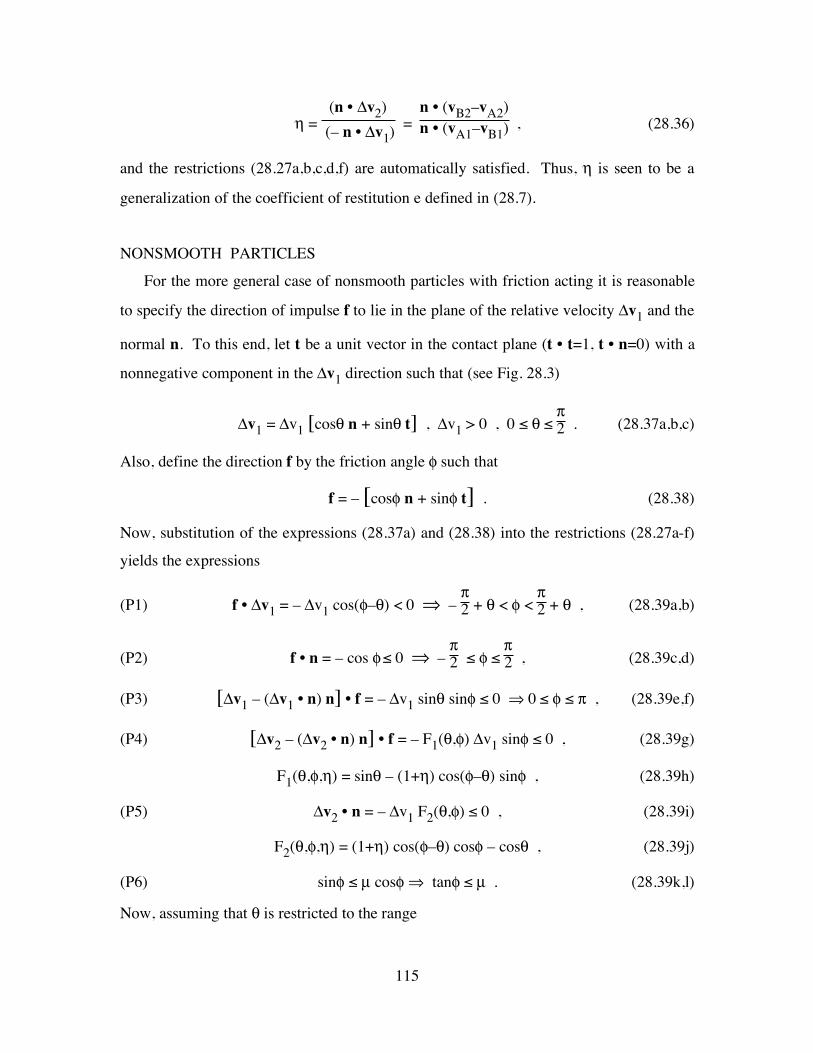
115
η = (n • Δv2)
(– n • Δv1) = n • (vB2–vA2)n • (vA1–vB1) , (28.36)
and the restrictions (28.27a,b,c,d,f) are automatically satisfied. Thus, η is seen to be a
generalization of the coefficient of restitution e defined in (28.7).
NONSMOOTH PARTICLES
For the more general case of nonsmooth particles with friction acting it is reasonable
to specify the direction of impulse f to lie in the plane of the relative velocity Δv1 and the
normal n. To this end, let t be a unit vector in the contact plane (t • t=1, t • n=0) with a
nonnegative component in the Δv1 direction such that (see Fig. 28.3)
Δv1 = Δv1 [cosθ n + sinθ t] , Δv1 > 0 , 0 ≤ θ ≤ π2 . (28.37a,b,c)
Also, define the direction f by the friction angle φ such that
f = – [cosφ n + sinφ t] . (28.38)
Now, substitution of the expressions (28.37a) and (28.38) into the restrictions (28.27a-f)
yields the expressions
(P1) f • Δv1 = – Δv1 cos(φ–θ) < 0 ⇒ – π2 + θ < φ <
π2 + θ , (28.39a,b)
(P2) f • n = – cos φ ≤ 0 ⇒ – π2 ≤ φ ≤
π2 , (28.39c,d)
(P3) [Δv1 – (Δv1 • n) n] • f = – Δv1 sinθ sinφ ≤ 0 ⇒ 0 ≤ φ ≤ π , (28.39e,f)
(P4) [Δv2 – (Δv2 • n) n] • f = – F1(θ,φ) Δv1 sinφ ≤ 0 , (28.39g)
F1(θ,φ,η) = sinθ – (1+η) cos(φ–θ) sinφ , (28.39h)
(P5) Δv2 • n = – Δv1 F2(θ,φ) ≤ 0 , (28.39i)
F2(θ,φ,η) = (1+η) cos(φ–θ) cosφ – cosθ , (28.39j)
(P6) sinφ ≤ µ cosφ ⇒ tanφ ≤ µ . (28.39k,l)
Now, assuming that θ is restricted to the range

116
0 ≤ θ ≤ π2 , (28.40)
the restrictions (28.39a,c,e) are satisfied whenever φ lies in the range
0 ≤ φ < π2 , (28.41)
and the restrictions (28.39g) and (28.39i) require the functions F1 and F2 to be
nonnegative
F1(θ,φ,η) ≥ 0 , F2(θ,φ,η) ≥ 0 . (28.42)
However, it can be seen that at the boundary φ=π/2 these functions are negative
F1(θ,π2,η) = sinθ – (1+η) sinθ = – η sinθ < 0 , F2(θ,
π2,η) = – cosθ < 0 , (28.43)
so that the conditions (28.42g,i) are violated. Moreover, let φ1, φ2 and φ3 be positive
values of φ less than π/2 which define the boundaries of the restrictions (28.42g,i,l), such
that
F1(θ,φ1,η) = 0 , F2(θ,φ2,η) = 0 , tanφ3 = µ . (28.44)
It then follows that
φ1 ≤ π2 , φ2 ≤
π2 . (28.45)
Moreover, with the help of (28.39h) it can be shown that
F1(θ,θ,η) = – η sinθ ≤ 0 , (28.46)
so that φ1can be further restricted
φ1 ≤ θ . (28.47)
Next, using (28.39h) and (28.39j) it can be shown that
F2(θ,φ1,η) = [ sinθsinφ1
] cosφ1 – cosθ = [cotφ1 – cotθ] sinθ ≥ 0 , (28.48)
so that the maximum value φmax of φ is controlled by either the condition (28.39g) that
the impulsive force resists slip at the end of the impact or the Coulomb friction condition
(28.39l). This means that the range of φ should be limited to
0 ≤ φ ≤ φmax= Min(φ1,φ3) . (28.49)
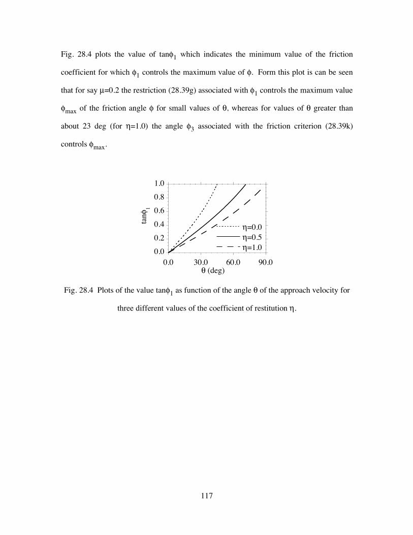
117
Fig. 28.4 plots the value of tanφ1 which indicates the minimum value of the friction
coefficient for which φ1 controls the maximum value of φ. Form this plot is can be seen
that for say µ=0.2 the restriction (28.39g) associated with φ1 controls the maximum value
φmax of the friction angle φ for small values of θ, whereas for values of θ greater than
about 23 deg (for η=1.0) the angle φ3 associated with the friction criterion (28.39k)
controls φmax.
0.0
0.2
0.4
0.6
0.8
1.0
!=0.0
!=0.5
!=1.0
0.0 30.0 60.0 90.0
tan"
1
# (deg)
Fig. 28.4 Plots of the value tanφ1 as function of the angle θ of the approach velocity for
three different values of the coefficient of restitution η.

118
29. Equations Of Motion Of A Rigid Body
Fig. 29.1
To describe the dynamics of rigid bodies we define the mass m, linear momentum G,
angular momentum Ho (about the origin). Motivated by the definitions of m, G, Ho for a
system of particles we replace the summation process by integration over the body of an
elemental mass dm and write
m = ∫ dm , (29.1a)
G = ∫ v dm , (29.1b)
Ho = ∫ x × v dm , (29.1c)
where v is the linear momentum per unit mass, and x × v is the angular momentum (about
the origin) per unit mass. In rigid body dynamics we define two types of external forces
that act on the body: (1) body forces per unit mass denoted by the vector b (like the force
of gravity), and (2) concentrated forces Fi acting at the points xi (see Fig. 29.1). Then the
resultant external force F applied to the rigid body is given by
F =∫ b dm + ∑i=1
N Fi . (29.2)
Similarly, the resultant moment Mo (about the origin) is given by
e2 e1
e3 x1
O
xN F1
M1
MM
FN b

119
Mo = ∫ x × b dm + ∑i=1
N xi × Fi + ∑
i=1
M Mi , (29.3)
where Mi (i=1,2,...,M) are M moments applied to the rigid body at various points.
We now assume that the equations of motion of a rigid body have the same form as
those for a single particle and a simple system of particles so we postulate the
conservation of mass
•m = 0 , (29.4)
the balance of linear momentum
•G = F , (29.5)
and the balance of angular momentum
•Ho = Mo . (29.6)
Notice that these balance laws are postulated instead of being derived directly from the
dynamics of a system of particles, and they are consistent with the dynamics of a system
of particles if the internal forces are such that they apply no net moment mo to the body.
Ultimately the validity of these assumptions can only be verified by comparing
theoretical predictions with results of experiments. In this regard, we note that numerous
experiments have proven these equations of motion of a rigid body to be quite accurate
for nonrelativistic velocities. In fact, the generalizations (29.4)-(29.6) hold even for
continuous deformable media like fluids and elastic solids.
It is important to emphasize that since a rigid body has six degrees of freedom (three
translational characterized by the position vector of a point on the body, and three
rotational characterized by the angular velocity vector) both the balances of linear
momentum and angular momentum must be used to determine the position of a point on
the body and its angular orientation in space. This should be contrasted with the fact that
the balance of angular momentum of a single particle was derived as a theorem using the
balance of linear momentum, so the balance of angular momentum contains no
information that is not already contained in the balance of linear momentum.

120
In our study of dynamics of rigid bodies we will confine attention to values of b
which are constant (like the case of a constant gravitational field, e.g. b = – g e3). For
this case the body force Fb and the moment Mbo of the body force may be expressed in
the simple forms
Fb = ∫ b dm = m b , Mbo = ∫ x × b dm = –x × m b , (29.7)
where –x denotes the location of the center of mass of the body
m –x = ∫ x dm . (29.8)
The results (29.7) indicates that when b is constant the body force Fb is merely the total
mass of the body m times b and the body force Fb acts at the center of mass of the body.
This proves that the gravitational force acts through the center of mass of the body.
Fig. 29.2
Sometimes it is convenient to refer the equations of motion to a moving point. To
this end we let X be the position vector from the fixed origin to an arbitrary moving point
B and let p be the vector from B to any material point in the body (see Fig. 29.2) so that
x = X + p , –x = X + –p , xi = X + pi , (29.9a,b,c)
where –p is the location of the center of mass of the body relative to B. Using (29.1b) and
differentiating (29.8) we may deduce that the linear momentum of a rigid body is the
mass of the body times the absolute velocity of its center of mass
e2 e1
e3 x
O
–x
p
X
b
cm
–p
B

121
G = m –v . (29.10)
Now, with the help of (29.9) and (29.10) the balance of linear momentum (29.5) may be
written in the alternative form
m (••X + ••–p) = F . (29.11)
This is identical to equation (25.5) for a system of particles so it follows that the balance
of linear momentum of a rigid body remains invariant (unchanged in form) to a
superposed constant velocity •X [see equation (25.6)].
To develop the alternative form of the balance of angular momentum we substitute
(29.9a) into the definition (29.1c) and obtain the expressions
Ho = ∫ (X + p) × v dm = X × ∫ v dm + ∫ p × v dm ,
Ho = X × m –v + ∫ p × ( •X + •p) dm ,
Ho = X × m –v + ∫ p dm × •X + ∫ p × •p dm ,
Ho = X × m –v + m –p × •X + HB , (29.12)
where HB is the relative angular momentum about the point B
HB = ∫ p × •p dm . (29.13)
Furthermore, following the development of (25.9) we may differentiate (29.12) to obtain
•Ho = X × F + m –p × ••X + •HB . (29.14)
Now, substituting (29.9a,c) into (29.3), the expression for the moment Mo about the
origin becomes
Mo = ∫ (X + p) × b dm + ∑i=1
N (X + pi) × Fi + ∑
i=1
M Mi ,
Mo = X × [∫ b dm + ∑i=1
N Fi] + ∫ p × b dm + ∑
i=1
N pi × Fi + ∑
i=1
M Mi ,

122
Mo = X × F + MB , (29.15)
where the moment MB of the external forces about the point B is defined by
MB = ∫ p × b dm + ∑i=1
N pi × Fi + ∑
i=1
M Mi . (29.16)
Furthermore, if b is constant then (29.16) reduces to
MB = ∫ p dm × b + ∑i=1
N pi × Fi + ∑
i=1
M Mi ,
MB = –p × m b + ∑i=1
N pi × Fi + ∑
i=1
M Mi , (29.17)
which shows that b acts through the center of mass. Finally, substitution of (29.14) and
(29.15) into (29.6) yields the balance of angular momentum in the alternative form
•HB + m –p × ••X = MB . (29.18)
Notice that for a general moving point B the balance of angular momentum changes
form. However, for the special case when –p × ••X vanishes, the balance of angular
momentum remains invariant with
•HB = MB for –p × ••X = 0 . (29.19)
This happens for the following three cases.
Case I: The point B moves with constant velocity
•X = constant , (29.20)
so the balance of angular momentum remains invariant to a superposed constant velocity.
Case II: The point B is the center of mass of the system
–p = 0 , (29.21)
and the balance of angular momentum may be written in the form
–•H = –M , (29.22)

123
where for convenience we have denoted the value of HB by –H and the value of MB by
–M, so that –H is the relative angular momentum about the center of mass and –M is the
moment due to external forces about the center of mass. It is important to emphasize that
equation (29.22) holds even when the center of mass accelerates.
Case III: The point B accelerates towards or away from the center of mass
••X | | –p . (29.23)
Before closing this section it is convenient to use the result (29.12) and consider the
special case when B is taken to be the center of mass with
X = –x , –p = 0 , (29.24a,b)
HB = –H = ∫ (x – –x) × (v – –v) dm , (29.24c)
to derive the result that
Ho = (–x × m –v) + –H . (29.25)
This means that the angular momentum about the origin O is equal to the sum of the
angular momentum of the center of mass (–x × m –v) about O and the angular momentum
–H of the rigid body about its center of mass. Also, we may solve (29.12) for HB and
substitute (29.25) into the resulting expression to obtain
HB = Ho – X × m –v – m –p × •X = (–x × m –v) + –H – X × m –v – m –p × •X ,
HB = (X + –p) × m –v + –H – X × m –v – m –p × •X ,
HB = –p × m –v + –H – m –p × •X = –p × m ( •X + –•p) + –H – m –p × •X ,
HB = –p × m –•p + –H . (29.26)
which is similar to (29.25).
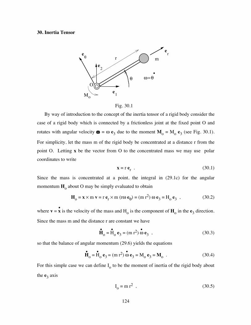
124
30. Inertia Tensor
e1
e2
O
m
e!
er
!
Mo
r
" = !
•
Fig. 30.1
By way of introduction to the concept of the inertia tensor of a rigid body consider the
case of a rigid body which is connected by a frictionless joint at the fixed point O and
rotates with angular velocity ω = ω e3 due to the moment Mo = Mo e3 (see Fig. 30.1).
For simplicity, let the mass m of the rigid body be concentrated at a distance r from the
point O. Letting x be the vector from O to the concentrated mass we may use polar
coordinates to write
x = r er . (30.1)
Since the mass is concentrated at a point, the integral in (29.1c) for the angular
momentum Ho about O may be simply evaluated to obtain
Ho = x × m v = r er × m (rω eθ) = (m r2) ω e3 = Ho e3 , (30.2)
where v = •x is the velocity of the mass and Ho is the component of Ho in the e3 direction.
Since the mass m and the distance r are constant we have
•Ho = •Ho e3 = (m r2) •ω e3 , (30.3)
so that the balance of angular momentum (29.6) yields the equations
•Ho = •Ho e3 = (m r2) •ω e3 = Mo e3 = Mo . (30.4)
For this simple case we can define Io to be the moment of inertia of the rigid body about
the e3 axis
Io = m r2 , (30.5)

125
and write the angular momentum Ho in the form
Ho = Io ω , (30.6)
and the balance of angular momentum in the scalar form
•Ho = Mo . (30.7)
e1
e2
O
!
•I = m k
2
Fig. 30.2
Formulas of the type (30.6) and (30.7) hold for special cases of a rigid body rotating
about the e3 axis even when the mass is not concentrated (see Fig. 30.2). For this case we
sometimes use the analogy of a concentrated mass (30.5) and define the radius of
gyration k by the formulas
Io = m k2 , k = [Iom]
1/2 . (30.8)
Thus the radius of gyration k is the radius at which the mass of the body would have to be
concentrated in order to obtain the correct value of the moment of inertia Io for rotation
about the origin.
To describe three-dimensional motion of a rigid body we must generalize the scalar
equation (30.6) to a vector equation. It will be shown presently that the appropriate
vector equation can be written in the form
Ho = Io ω , (30.9)
where ω is the angular velocity vector of the rigid body and Io is the inertia tensor of the
rigid body about the point O. The inertia tensor Io is a second order tensor that operates

126
on the vector ω to give the vector Ho. Writing (30.9) in the component form relative to
the basis ei
Hoi ei = Ioij ωj ei , Hoi = Ioij ωj , (30.10a,b)
we may observe that the (i,j) components Ioij of Io may be identified as a square matrix
so that (30.10) merely represents a matrix Ioij multiplying a vector ωj to obtain another
vector Hoi. More generally the angular momentum –H about the center of mass can be
written in terms of the inertia –I about the center of mass
–H = –I ω . (30.12a)
If B is an arbitrary material point attached to the body then the angular momentum
HB can also be expressed in terms of the inertia IB about B in a form similar to (30.12),
such that
HB = ∫ p × •p dm = IB ω , HBi = IBij ωj , (30.13a,b)
where p is the vector from the point B to any point in the body. Since B is a material
point and the vector p connects two material points on the rigid body it follows that
•p = ω × p , (30.14)
so that (30.13) may be written in the form
HB = ∫ p × (ω × p) dm = ∫ [(p • p) ω – (p • ω) p] dm . (30.15)
It is important to note that the angular velocity ω(t) is a function of time only so it is not
affected by the integration over the mass of the body and therefore ω can be factored out
of the integral. This can be done by defining the tensor product ⊗ such that for any
vectors a,b,c, the quantity (a ⊗ b) is a second order tensor and d = (a ⊗ b) c is a vector
having the properties
d = (a ⊗ b) c = a (b • c) = (b • c) a , (30.16a)
di = (ai bj) cj = ai (bj cj) = (bj cj) ai . (30.16b)
Thus, we may write

127
(p • ω) p = (p ⊗ p) ω , ω = I ω , (30.17a,b)
where I denotes the unit tensor and should not be confused with inertia tensors which are
denoted by the same symbol with either an over bar –I or a subscript IB. Now
substituting (30.17) into (30.15) we may deduce that
HB = IB ω , IB = ∫ [(p • p) I – (p ⊗ p)] dm . (30.18a,b)
Notice that the inertia tensor IB is a property of the body and is independent of the
motion of the body. It follows that it is most convenient to calculate the components of
IB relative to a body coordinate system ei' which rotates with the body
•ei' = ω × ei' . (30.19)
Letting pi' = ei' • p be the coordinates of the body coordinate system, P' be the region of
space occupied by the body, dV = (dp1' dp2' dp3' ) be the element of volume, and ρ(p1' ) be
the positive mass density (mass per unit volume), we may write
IB = ∫P' ρ [(p • p) I – (p ⊗ p)] dV , (30.20a)
IB' ij = ∫P' ρ [(pm' pm' ) δij – (pi' pj')] dV , (30.20b)
where the Kronecker delta δij are the components of the unit tensor I and IB' ij are the
components of IB relative to the basis ei'. Notice that since we have chosen a body
coordinate system the limits of integration in (30.20b) are independent of time
(independent of the motion of the body).
In view of either of the representations (30.20a,b) it can be seen that the inertia tensor
IB is a symmetric tensor (i.e. its transpose IBT is equal to itself)
IBT = IB , IBji = IBij , (30.21a,b)
and it is a positive definite tensor. By positive definite we mean that for an arbitrary
nonzero constant vector a the scalar product a • IB a is positive
a • IB a = ai IBij aj > 0 for a ≠ 0 . (30.22)
This can be proved by substituting (30.20a) into (30.22) to obtain

128
a • IB a =∫P'ρ [(p • p) (a • a) – (p • a)(p • a)] dV > 0 , (30.23)
which is positive since the constant vector a can only be equal to p at at most one point in
the body.
In order to discuss the physical meaning of the inertia tensor IB it is convenient to
consider the expanded forms of the components (30.20b). In particular the diagonal
components may be written in the forms
IB' 11 = ∫P' ρ [ (p2' )2 + (p3' )
2 ] dV , (30.24a)
IB' 22 = ∫P' ρ [ (p1' )2 + (p3' )
2 ] dV , (30.24b)
IB' 33 = ∫P' ρ [ (p1' )2 + (p2' )
2 ] dV , (30.24c)
and the off-diagonal components may be written as
IB' 12 = – ∫P' ρ [ p1' p2' ] dV , (30.25a)
IB' 13 = – ∫P' ρ [ p1' p3' ] dV , (30.25a)
IB' 23 = – ∫P' ρ [ p2' p3' ] dV , (30.25a)
Physically the integrands of the diagonal components of inertia can be interpreted as the
square of the distance of the material point from the coordinate axes ei'.
It is also convenient to expand equation (30.12c) for the angular momentum to obtain
HB' i = IB' i1 ω1' + IB' i2 ω2' + IB' i3 ω3' , (30.26a)
⎝⎜⎜⎛
⎠⎟⎟⎞
HB' 1HB' 2HB' 3
= ⎝⎜⎜⎛
⎠⎟⎟⎞IB' 11 IB' 12 IB' 13
IB' 12 IB' 22 IB' 23IB' 13 IB' 23 IB' 33
⎝⎜⎛
⎠⎟⎞ω1'
ω2'ω3'
. (30.26b)
Notice from (30.26b) that in general the inertia tensor has six independent
components and the angular momentum vector has a different direction from the angular
velocity vector. This means that if you rotate the body about a given direction then in

129
general you will get angular momentum components in the direction of rotation and in
the plane normal to the rotation. From a physical point of view it makes sense to ask the
question whether there are special directions in which you can rotate the body and only
get angular momentum in the direction of rotation. For this case we would have
HB = IB ω = I ω , HB' i = IB' ij ωj' = I ωi' , (30.27a,b)
where I is a scalar to be determined. Rewriting (30.27) we have
(IB – I I) ω = 0 , (IB' ij – I δij) ωj' = 0 , (30.28a,b)
or in expanded form
⎝⎜⎜⎛
⎠⎟⎟⎞IB' 11–I IB' 12 IB' 13
IB' 12 IB' 22–I IB' 23IB' 13 IB' 23 IB' 33–I
⎝⎜⎛
⎠⎟⎞ω1'
ω2'ω3'
= ⎝⎜⎜⎛
⎠⎟⎟⎞
000 . (30.29)
Thus, we have reduced the problem to a standard eigenvalue problem. Since the tensor
IB' ij is real and symmetric there exists three eigenvalues I which are determined by the
characteristic equation
det (IB' ij – I δij) = 0 , (30.30)
and three associated eigenvectors which are determined by solving (30.29) for the
associated directions of ωi'. These eigenvectors can be ordered to form a right-handed
orthonormal set of vectors which we denote by ei''. Then letting IBi'' j be the components of
IB relative to ei'' we have
IBi'' j = ⎝⎜⎜⎛
⎠⎟⎟⎞IB1'' 1 0 0
0 IB2'' 2 00 0 IB3'' 3
, (30.31)
with IB1'' 1, IB2'' 2, IB3'' 3 being positive constants, since for example
IB1'' 1 = ∫P' ρ [ (p2' ')2 + (p3' ')
2 ] dV . (30.32)
Sometimes the eigenvalues are called principal values and the eigenvectors are called
principal directions of the tensor IB.
In general the components IB' ij relative to ei', and IBi'' j relative to ei'' of the tensor IB
must satisfy tensor transformation rules in order for IB to be independent of our choice of
130
the coordinate system. In particular, let Aij be the transformation tensor (direction
cosines) characterizing the relationship between the orientations of ei' and ei'' such that
Aij = ei'' • ej' , ei'' = Aij ej' , ei' = Aji ej'' . (30.33a,b,c)
Notice that by definition the first index of Aij always refers to the double primed system
and the second index always refers to the single primed system. It follows that Aij is an
orthogonal tensor because
δij = ei'' • ej'' = Aim em' • Ajn en' = Aim Ajn δmn = Aim Ajm = Aim AmT
j , (30.34a)
δij = ei' • ej' = Ami em' ' • Anj en' ' = Ami Anj δmn = Ami Amj = A iT
m Amj . (30.34b)
Recalling that the components of IB satisfy the equations
IB' ij = ei' • IB ej' , IBi'' j = ei'' • IB ej'' , (30.35a,b)
we may use (30.33) to derive the transformation relations
IBi'' j = Aim em' • IB Ajn en' = Aim (em' • IB en' ) Ajn , (30.36a)
IBi'' j = Aim IB' mn Ajn = Aim IB' mn AnT
j , (30.36b)
⎝⎜⎜⎛
⎠⎟⎟⎞IB1'' 1 IB1'' 2 IB1'' 3
IB1'' 2 IB2'' 2 IB2'' 3IB1'' 3 IB2'' 3 IB3'' 3
= ⎝⎜⎜⎛
⎠⎟⎟⎞A11 A12 A13
A21 A22 A23A31 A32 A33
⎝⎜⎜⎛
⎠⎟⎟⎞IB' 11 IB' 12 IB' 13
IB' 12 IB' 22 IB' 23IB' 13 IB' 23 IB' 33
⎝⎜⎜⎛
⎠⎟⎟⎞A11 A21 A31
A12 A22 A32A13 A23 A33
(30.36c)
and
IB' ij = Ami em' ' • IB Anj em' ' = Aim (em' ' • IB em' ') Anj , (30.37a)
IB' ij = Ami IBm'' n Anj = A iT
m IBm'' n Anj , (30.37b)
⎝⎜⎜⎛
⎠⎟⎟⎞IB' 11 IB' 12 IB' 13
IB' 12 IB' 22 IB' 23IB' 13 IB' 23 IB' 33
= ⎝⎜⎜⎛
⎠⎟⎟⎞A11 A21 A31
A12 A22 A32A13 A23 A33
⎝⎜⎜⎛
⎠⎟⎟⎞IB1'' 1 IB1'' 2 IB1'' 3
IB1'' 2 IB2'' 2 IB2'' 3IB1'' 3 IB2'' 3 IB3'' 1
⎝⎜⎜⎛
⎠⎟⎟⎞A11 A12 A13
A21 A22 A23A31 A32 A33
(30.37c)
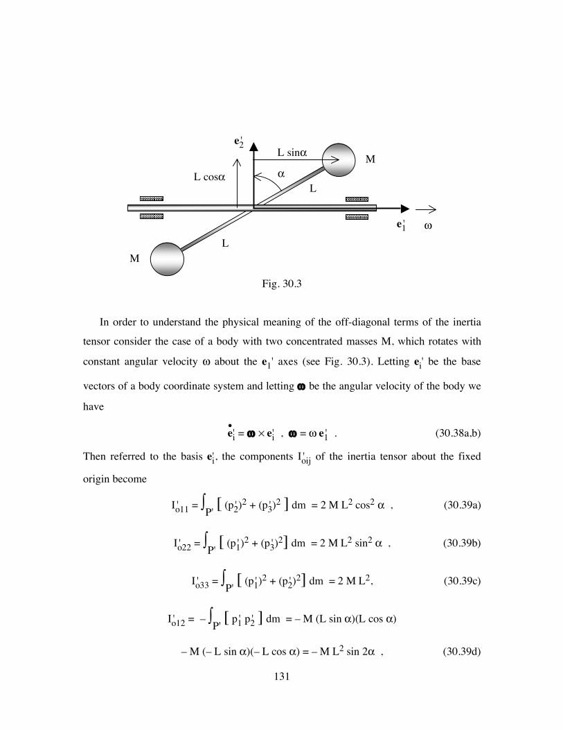
131
Fig. 30.3
In order to understand the physical meaning of the off-diagonal terms of the inertia
tensor consider the case of a body with two concentrated masses M, which rotates with
constant angular velocity ω about the e1' axes (see Fig. 30.3). Letting ei' be the base
vectors of a body coordinate system and letting ω be the angular velocity of the body we
have
•ei' = ω × ei' , ω = ω e1' . (30.38a,b)
Then referred to the basis ei', the components Io' ij of the inertia tensor about the fixed
origin become
Io'11 = ∫P' [ (p2' )2 + (p3' )
2 ] dm = 2 M L2 cos2 α , (30.39a)
Io'22 = ∫P' [ (p1' )2 + (p3' )
2] dm = 2 M L2 sin2 α , (30.39b)
Io'33 = ∫P' [ (p1' )2 + (p2' )
2] dm = 2 M L2, (30.39c)
Io'12 = – ∫P' [ p1' p2' ] dm = – M (L sin α)(L cos α)
– M (– L sin α)(– L cos α) = – M L2 sin 2α , (30.39d)
e1'
e2'
ω L
L
L sinα
L cosα α M
M
132
Io'13 = – ∫P' [ p1' p3' ] dm = 0 , (30.39e)
Io'23 = – ∫P' [ p2' p3' ] dm = 0 , (30.39f)
since the masses are located in the p3' = 0 plane. Substituting (30.38b) and (30.39) into
(30.10) the angular momentum Ho may be written in the form
Ho = Io' ij ωj' ei' = Io' i1 ω ei' = (Io'11 ω) e1' + (Io'21 ω) e2' + (Io'31 ω) e3' ,
Ho = (2 M L2 cos2 α) ω e1' – (M L2 sin 2α) ω e2' . (30.40)
Notice first that the off-diagonal term Io'12 causes the angular momentum Ho to have a
term in the e2' direction even though the body is only rotating about the e1' direction.
Recalling that Ho is expressed in terms of the rotating basis ei', the rate of change of
angular momentum becomes
•Ho = ω × Ho = – (M L2 sin 2α) ω2 e3' , (30.41)
since ω is constant. Thus the balance of angular momentum (29.6) yields an expression
for the moment Mo applied to the body of the form
Mo = Io'12 ω2 e3' = – (M L2 sin 2α) ω2 e3' . (30.42)
Notice from (30.42) that if the angle α vanishes then ei' are principal axes of inertia so
the off-diagonal terms of the inertia tensor vanish and there is no moment required to
rotate the body with constant angular velocity about the principal e1' axes. This means
that in general there is no moment required to rotate a body with constant angular
velocity about any of its principal directions. Notice also, that if 0 < α < π/2 then the
moment Mo is directed along the negative e3' axes which is consistent with the physical
notion that if masses were allowed to rotate freely in the e1' –e2' plane then the angle α
would tend to zero.

133
Fig. 30.4
Since we can always choose a body coordinate system in which the inertia tensor is
diagonalized it is of interest to reconsider the previous example and examine what
simplification and complications occur when we refer all tensors to the vectors ei'' which
are oriented along the principal directions of the body (see Fig. 30.4). For this case the
base vectors ei'' also rotate with angular velocity ω such that
•ei'' = ω × ei'' , ω = ω (cos α e1' ' + sin α e2' ') . (30.43a,b)
Since ei'' are principal axes of inertia the components Ioi'' j of the inertia tensor referred to
ei'' become
Io1'' 1 = Io3'' 3 = 2 M L2 , Io2'' 2 = Io1'' 2 = Io1'' 3 = Io2'' 3 = 0 . (30.44a,b)
Recalling that any vector or tensor can be referred to any coordinate system, the angular
momentum vector Ho may be written in the form
Ho = Io' i'j ωi'' ei'' = (Io1'' 1 ω1' ') e1' ' + (Io2'' 2 ω2' ') e2' ' + (Io3'' 3 ω3' ') e3' ' ,
Ho = (Io1'' 1 ω1' ') e1' ' = (2 M L2) (ω cos α) e1' ' . (30.45)
Since ω is constant we have
•Ho = ω × Ho = – (M L2 sin 2α) ω2 e3'' , (30.46)
e1'
e2'
ω L
L
L sinα
L cosα α M
M e1''
e2''
134
which gives the same moment Mo as in (30.42). Notice that here the components Io' i'j of
the inertia tensor are simple but the components of the angular velocity ω referred to ei''
are more complicated. Since both choices of the coordinate system yield rather simple
analyses the particular choice becomes merely a matter of preference.

135
31. Transfer Theorem For The Inertia Tensor
P1
P2
PN
•B
e '1
e '2
e '3
Fig. 31.1
If a body is composed of N parts PI' (I=1,2,...,N) (see Fig. 31.1), then by the additive
property of integration we obtain the additive property of the inertia tensor referred to an
arbitrary point B in the body
P' = P1'∪ P2'∪...∪PN' , (31.1a)
IB = 1IB + 2IB + ... + NIB , (31.1b)
where IB is the inertia tensor of the whole body relative to B and IIB is the inertia tensor
of the part PI' of body relative to B
IB = ∫P ρ [(p • p) I – p⊗p] dV , (31.2a)
IIB = ∫PI ρ [(p • p) I – p⊗p] dV . (31.2b)
Furthermore letting IB' ij be the components of IB and IIB' ij be the components of IIB
relative to the body base vectors ei' we have
IB' ij = 1IB' ij + 2IB' ij + ... + NIB' ij . (31.3)
It is important to emphasize that the components of tensors can only be added if they are
referred to the same base vectors.
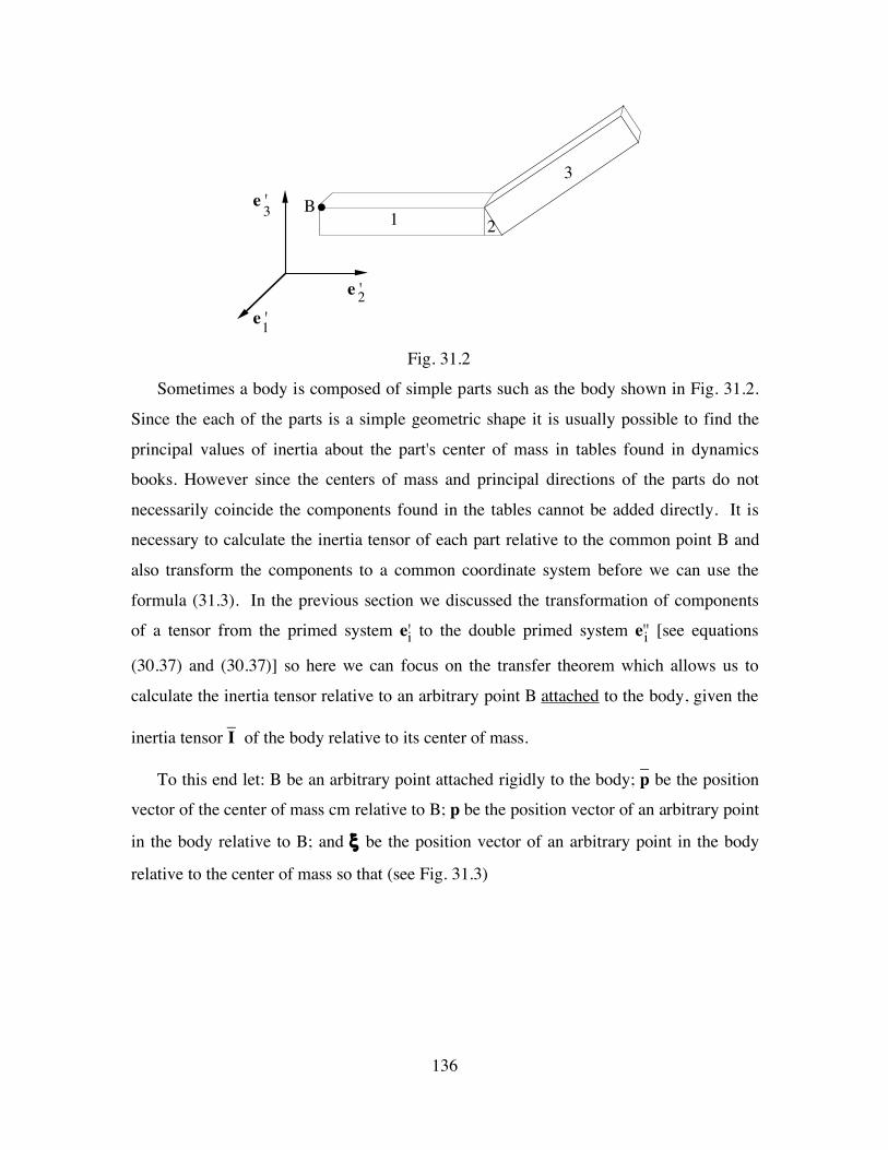
136
e '1
e '2
e '3 •B
12
3
Fig. 31.2
Sometimes a body is composed of simple parts such as the body shown in Fig. 31.2.
Since the each of the parts is a simple geometric shape it is usually possible to find the
principal values of inertia about the part's center of mass in tables found in dynamics
books. However since the centers of mass and principal directions of the parts do not
necessarily coincide the components found in the tables cannot be added directly. It is
necessary to calculate the inertia tensor of each part relative to the common point B and
also transform the components to a common coordinate system before we can use the
formula (31.3). In the previous section we discussed the transformation of components
of a tensor from the primed system ei' to the double primed system ei'' [see equations
(30.37) and (30.37)] so here we can focus on the transfer theorem which allows us to
calculate the inertia tensor relative to an arbitrary point B attached to the body, given the
inertia tensor –I of the body relative to its center of mass.
To this end let: B be an arbitrary point attached rigidly to the body; –p be the position
vector of the center of mass cm relative to B; p be the position vector of an arbitrary point
in the body relative to B; and ξ be the position vector of an arbitrary point in the body
relative to the center of mass so that (see Fig. 31.3)

137
Fig. 31.3
p = –p + ξ . (31.4)
Using the formula (31.2a) for IB, and the representation (31.4) we may write
IB = ∫P ρ [{(–p + ξ ) • (–p + ξ )} I – (–p + ξ )⊗(–p + ξ ) ] dV ,
IB = ∫P ρ [(–p • –p + 2 –p • ξ + ξ • ξ ) I – (–p⊗–p + –p⊗ξ + ξ⊗–p+ ξ ⊗ξ ) ] dV ,
IB = ∫P ρ [(ξ • ξ ) I – ξ⊗ξ ] dV + ∫P ρ [(–p • –p) I – –p⊗–p] dV
+ ∫P ρ [(2–p • ξ ) I – (–p⊗ξ + ξ⊗–p) ] dV , (31.5)
However, since ξ is measured from the center of mass of the body
∫P ρ ξ dV = 0 , (31.6)
and –p is independent of the integration equation (31.5) reduces to
IB = m [(–p • –p) I – –p⊗–p] + –I , (31.7)
where –I is the inertia tensor relative to the center of mass. This is the transfer theorem
for the inertia tensor. Now, if we refer all tensors to the base vectors ei' we may write the
component form of (31.7) as
e2 e1
e3
x
O
–x
p
cm –p
B
e1'
e2' e3'
ξ
xB
138
IB' ij = –Iij' + m [(–pm' –pm' ) δij – –pi' –pj'] , (31.8a)
and the expanded form as
IB' 11 = –I11' + m [(–p2' )2 + (–p3' )
2] , (31.9a)
IB' 22 = –I22' + m [(–p1' )2 + (–p3' )
2] , (31.9b)
IB' 33 = –I33' + m [(–p1' )2 + (–p2' )
2] , (31.9c)
IB' 12 = –I12' – m [–p1' –p2' ] , (31.9d)
IB' 13 = –I13' – m [–p1' –p3' ] , (31.9e)
IB' 23 = –I23' – m [–p2' –p3' ] . (31.9f)
Notice that even if ei' are parallel to the principal directions of inertia about the center of
mass (i.e. –Iij' is a diagonal tensor) they may no longer be parallel to the principal
directions of inertia relative to the point B (i.e. IB' ij may not be a diagonal tensor).
Finally, we emphasize that although equation (31.7) holds even if the point B is not
rigidly attached to the body the resulting tensor IB cannot be used in the expression HB =
IB ω for the angular momentum of the body since then –p will not be a vector of constant
length rotating with angular velocity ω (i.e. •–p ≠ ω × –p).

139
32. Planar Motion
Fig. 32.1
GENERAL PLANAR MOTION
For general planar motion of a rigid body relative to the plane e1–e2 we require all
points in the rigid body to move in planes parallel to the plane e1–e2. Mathematically
this means the velocity of every point in the e3 direction vanishes
e3 • v = 0 . (32.1)
Letting: p be the position of an arbitrary point in the body relative to the center of mass;
–v be the velocity of the center of mass; and ω be the angular velocity of the rigid body,
the condition (32.1) requires
e3 • (–v + ω × p) = e3 • –v + (e3 × ω) • p = 0 , (32.2)
for every point p. It follows that for planar motion we require
e3 • –v = 0 , e3 × ω = 0 , (32.3a,b)
which means that the center of mass moves in the e1–e2 plane and the body only rotates
about the e3 direction so the angular velocity becomes
ω = ω e3 . (32.4)
Since the center of mass only moves in the plane it follows that it has no acceleration
in the e3 direction so from the balance of linear momentum we may deduce that the force
F is also planar with
F = F1 e1 + F2 e2 , –a = –a1 e1 + –a2 e2 . (32.5a,b)
e1
e2 X
–x
e1'
e2' ω
cm
140
Thus, for planar motion the balance of linear momentum reduces to the two scalar
equations
m –a1 = F1 , m –a2 = F2 . (32.6a,b)
We can also refer the vectors to the rotating body coordinate system ei' defined by
•ei' = ω × ei' , ω = ω e3 = ω e3' , (32.7a,b)
and write the balance of linear momentum in the form
m –a1' = F1' , m –a2' = F2' . (32.8a,b)
Letting –Iij' be the components of the inertia tensor –I relative to the center of mass we
may express the angular momentum –H relative to the center of mass in the form
–H = –I ω = –Iij' ωj' ei' = –Ii1' ω1' ei' + –Ii2' ω2' ei' + –Ii3' ω3' ei' ,
–H = –I ω = –Ii3' ω ei' = –I13' ω e1' + –I23' ω e2' + –I33' ω e3' . (32.9)
Thus, the rate of change of angular momentum becomes
–•H = δ
–Hδt + ω × –H =
δ–Hδt + ω e3' × –H . (32.10)
However since ei' is a body coordinate system the components –Iij' are constants so that
δ
–Hδt = –Ii3' •
ω ei' . (32.11)
Expanding the cross product in (32.10) we deduce that
–•H = (–I13'•ω – –I23' ω2) e1' + (–I23'
•ω + –I13' ω2) e2' + (–I33' •
ω) e3' . (32.12)
Thus, the component form of the balance of angular momentum (29.22) may be written
as
–I13'•ω – –I23' ω2 = –M1' , (32.13a)
–I23'•ω + –I13' ω2 = –M2' , (32.13b)
–I33' •ω = –M3' . (32.13c)
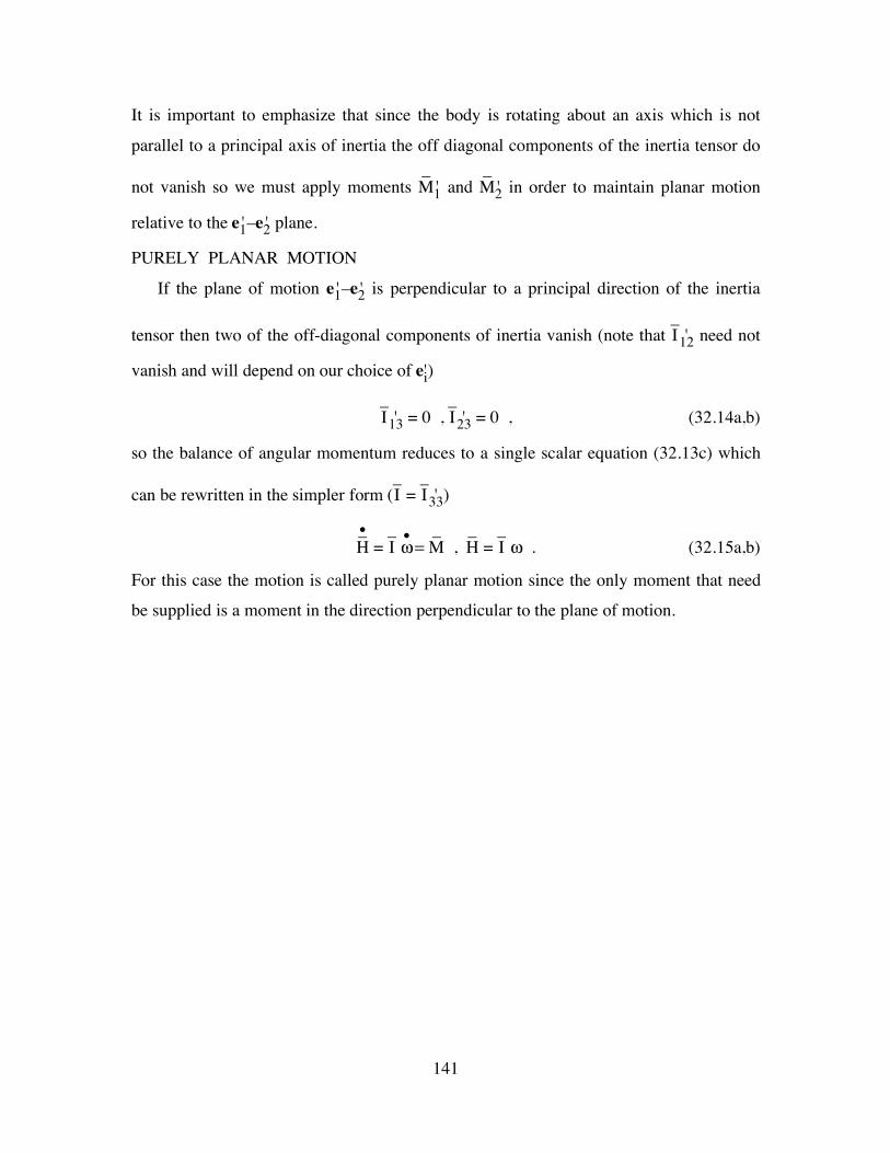
141
It is important to emphasize that since the body is rotating about an axis which is not
parallel to a principal axis of inertia the off diagonal components of the inertia tensor do
not vanish so we must apply moments –M1' and –M2' in order to maintain planar motion
relative to the e1' –e2' plane.
PURELY PLANAR MOTION
If the plane of motion e1' –e2' is perpendicular to a principal direction of the inertia
tensor then two of the off-diagonal components of inertia vanish (note that –I12' need not
vanish and will depend on our choice of ei')
–I13' = 0 , –I23' = 0 , (32.14a,b)
so the balance of angular momentum reduces to a single scalar equation (32.13c) which
can be rewritten in the simpler form (–I = –I33' )
–•H = –I •ω = –M , –H = –I ω . (32.15a,b)
For this case the motion is called purely planar motion since the only moment that need
be supplied is a moment in the direction perpendicular to the plane of motion.

142
33. Impulse On A Rigid Body
In view of the simplicity of the balance of linear momentum (29.5) and the two forms
of the balance of angular momentum (29.6) and (29.2) it follows that changes in
momentum from time t1 to time t2 can be determined by integrating these balance laws.
In particular, we can define the impulsive force F̂ and impulsive moments M̂o , –̂M such
that
F̂ = ∫t2 t1
F dt , (33.1a)
M̂o = ∫t2 t1
Mo dt , (33.1b)
–̂M = ∫t2 t1
–M dt . (33.1c)
so that integration of these balance laws yields the equations
F̂ = ∫t2 t1
•G dt = G2 – G1 , (33.2a)
M̂o = ∫t2 t1
•Ho dt = Ho2 – Ho1 , (33.2b)
–̂M = ∫t2 t1
–•H dt = –H2 – –H1 . (33.2c)
As an example let us consider the purely planar motion of a rigid body that is acted
upon by an impulsive force R̂ (see Fig. 33.1). The body has mass m, moment of inertia
–I = m –k2 about its center of mass and is initially at rest. The impulsive force R̂ is applied
in the constant e1 direction at the position x1 relative to the center of mass, such that
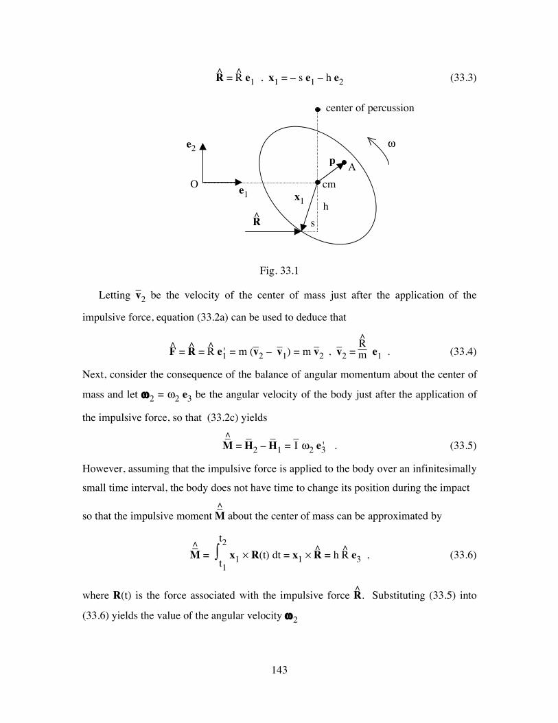
143
R̂ = R̂ e1 , x1 = – s e1 – h e2 (33.3)
Fig. 33.1
Letting –v2 be the velocity of the center of mass just after the application of the
impulsive force, equation (33.2a) can be used to deduce that
F̂ = R̂ = R̂ e1' = m (–v2 – –v1) = m –v2 , –v2 =
R̂m e1 . (33.4)
Next, consider the consequence of the balance of angular momentum about the center of
mass and let ω2 = ω2 e3 be the angular velocity of the body just after the application of
the impulsive force, so that (33.2c) yields
–̂M = –H2 – –H1 = –I ω2 e3' . (33.5)
However, assuming that the impulsive force is applied to the body over an infinitesimally
small time interval, the body does not have time to change its position during the impact
so that the impulsive moment –̂M about the center of mass can be approximated by
–̂M = ∫t2 t1
x1 × R(t) dt = x1 × R̂ = h R̂ e3 , (33.6)
where R(t) is the force associated with the impulsive force R̂. Substituting (33.5) into
(33.6) yields the value of the angular velocity ω2
R̂
e1
e2
s h
x1
p A cm
ω
center of percussion
O
144
ω2 = ω2 e3 , ω2 = h R̂–I
. (33.7a,b)
Now, assuming that no forces or moments are applied after the impact it follows that
the velocity –v of the center of mass and the angular velocity ω remain constant
–v = R̂m e1 , ω = ω e3 , ω =
h R̂–I
. (33.8)
Thus, the velocity vA of an arbitrary material point that is instantaneously located by the
position vector p relative to the center of mass is given by
vA = –v + •p = –v + ω × p = vA = R̂m e1 +
h R̂–I
e3 × (p1 e1 + p2 e2) ,
vA = [R̂m –
h R̂–I
p2] e1 + [h R̂–I
p1] e2 . (33.9)
Recall that the point A will locate the instantaneous center of zero velocity (vA = 0)
provided that {p1, p2} are given by
p1 = 0 , p2 = –I
m h = –k2h . (33.10a,b)
The result (33.10a) states that the instantaneous center of zero velocity lies along the line
perpendicular to the velocity of the center of mass of the body as it should. This point is
called the center of percussion because if the body were hinged there the impulsive
reaction at the hinge would vanish. Also, notice that the results (33.10) are valid for all
time so that instantaneous center of zero velocity is always located a distance p2 above
the center of mass and it moves with the constant velocity of the center of mass. In this
regard, it is emphasized that as the body rotates the material points that instantaneously
coincide with the instantaneous center of zero velocity change with time.
145
34. Energy Equation For A Rigid Body
Recall from (18.5) that we proved that for a single particle the rate of work of all
external forces is equal to the rate of change of kinetic energy
P = F • v = •T =
ddt [
12 m v • v] . (34.1)
Similarly we proved for a system of particles rigidly connected by central forces that the
internal forces do no work so the rate of work done by external forces again equals the
rate of change of kinetic energy [see (27.4) and (27.16)]
P = ∑i=1
N Fi • vi =
•T = ∑
i=1
N
•Ti , Ti =
12 mi vi • vi . (34.2a,b)
Before developing the energy equation for a rigid body it is desirable to first develop
an expression for the kinetic energy of the rigid body. It follows from the definition
(27.3b) for the kinetic energy of a system of particles that the kinetic energy of a rigid
body should be defined by
T = ∫ 12 v • v dm . (34.3)
Next, referring the motion to the center of mass we may write
x = –x + p , v = –v + •p = –v + ω × p , (34.4a,b)
where p is the vector from the center of mass –x to an arbitrary point in the body and ω is
the angular velocity of the body. It follows from (34.4b) that
v • v = (–v + ω × p) • (–v + ω × p) ,
v • v = –v • –v + 2 –v • (ω × p) + (ω × p) • (ω × p) ,
v • v = –v • –v + 2 –v • (ω × p) + ω • [ p × (ω × p) ] ,
v • v = –v • –v + 2 –v • (ω × p) + ω • [ (p • p) ω – (p • ω) p ] . (34.5)
Thus, the kinetic energy becomes
T = ∫ 12 –v • –v dm + 2 –v • [ω × ∫ 12 p dm]
+ 12 ω • ∫ [(p • p) ω – (p • ω) p] dm ,

146
T = 12 m –v • –v + –T , (34.6)
where the kinetic energy of motion relative to the center of mass –T is given by
–T = 12 ω • –H =
12 ω • –I ω =
12 ωi'
–I ij' ωj' . (34.7)
Note that in words, equation (34.6) states that the kinetic energy of the rigid body is equal
to the kinetic energy of the center of mass plus the kinetic energy of motion relative to
the center of mass.
If the body rotates about a fixed point O (see Fig. 34.1) then the kinetic energy T may
be expressed in the alternative form
T = ∫ 12 v • v dm = 12 ∫ (ω × x • v) dm =
12 ∫ (ω • x × v) dm ,
T = 12 ω • ∫ (x × v) dm =
12 ω • Ho =
12 ω • Io ω =
12 ωi'
–Io' ij ωj' . (34.8)
One of the differences between a rigid body and a system of particles is that it is
possible to apply external moments at points on a rigid body which can do work on the
body. Therefore, in order to develop the general form of the energy equation for a rigid
body we generalize the procedure used to obtain (34.2) which took the scalar product of
the equations of linear momentum of each particle with its associated velocity and
summed the result. Thus, for a rigid body we multiply the linear momentum equation
(29.5) by the velocity of the center of mass –v and multiply the balance of angular
momentum (29.22) by the angular velocity ω and sum the results to obtain
[∫ b dm + ∑i=1
N Fi ] •
–v + [∫ p × b dm + ∑i=1
N pi × Fi + ∑
i=1
M Mi] • ω
= m –•v • –v + –•H • ω , (34.9)
where pi is the vector measured from the center of mass to the point of application of the
force Fi. Using the properties of the scalar triple product and the fact that –v and ω are
functions of time only it is possible to rearrange this equation into the form
147
∫ b • (–v + ω × p) dm + ∑i=1
N Fi • (
–v + ω × pi) + ∑i=1
M Mi • ω = m –
•v • –v + –•H • ω . (34.10)
However, since p and pi are each vectors that connect two material points on the rigid
body it follows that the absolute velocity v of an arbitrary material point and the absolute
velocity vi of the point of application of the force Fi are given by
v = –v + ω × p , vi = –v + ω × pi , (34.11a,b)
so that (34.10) reduces to
∫ b • v dm + ∑i=1
N Fi • vi + ∑
i=1
M Mi • ω = m –
•v • –v + –•H • ω . (34.12)
Next, using (34.7) and the fact that ei' is a body coordinate system it may be shown that
–•T = ωi' –I ij'
•ωj' . (34.13)
Moreover, expressing –H in terms of its components relative to ei' we have
–H = –Iij' ωj' ei' , (34.14a)
–•H = δ
–Hδt + ω × –H , (34.14b)
–•H • ω = δ
–Hδt • ω = –Iij'
•ωj' ei' • ω = ωi'
–I ij' •ωj' = –
•T . (34.14c)
Thus, it follows that
m –•v • –v + –•H • ω = •T , (34.15)
so the energy equation for a rigid body may be written in the usual form
P = •T , (34.16)
where the mechanical power P is defined by
P = ∫ b • v dm + ∑i=1
N Fi • vi + ∑
i=1
M Mi • ω . (34.17)

148
For a uniform (independent of position) body force b, the rate of work of the body force
can be expressed in the simple form
∫ b • v dm = m b • –v , (34.18)
which is equivalent to an external force (m b) acting at the center of mass of the body.
Then, (34.17) reduces to the simpler form
P = mb • –v + ∑i=1
N Fi • vi + ∑
i=1
M Mi • ω . (34.19)
Here it is important to emphasize that the external forces Fi are multiplied by the absolute
velocities vi of the material points where they are applied and that all the external
moments Mi are multiplied by the same absolute angular velocity ω of the rigid body.
Using the form (34.19) of the mechanical power we may integrate the energy
equation (34.16) over the time interval [t1,t2] and write an energy equation in the form
–U2/1 = (T2 – T1) + (Vg2 – Vg1) + (Ve2 – Ve1) , (34.20)
where –U2/1 is the work done by all external forces which don't contribute to gravitational
potential energy Vg or elastic potential energy Ve and the work done by all external
moments.
Fig. 34.1
e1'
e2'
ω
O
e3'
x
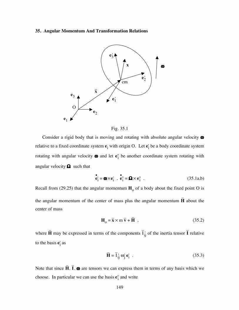
149
35. Angular Momentum And Transformation Relations
Fig. 35.1
Consider a rigid body that is moving and rotating with absolute angular velocity ω
relative to a fixed coordinate system ei with origin O. Let ei' be a body coordinate system
rotating with angular velocity ω and let ei'' be another coordinate system rotating with
angular velocity Ω such that
•ei' = ω × ei' , •ei'' = Ω × ei'' . (35.1a,b)
Recall from (29.25) that the angular momentum Ho of a body about the fixed point O is
the angular momentum of the center of mass plus the angular momentum –H about the
center of mass
Ho = –x × m –v + –H , (35.2)
where –H may be expressed in terms of the components –Iij' of the inertia tensor –I relative
to the basis ei' as
–H = –Iij' ωj' ei' . (35.3)
Note that since –H, –I, ω are tensors we can express them in terms of any basis which we
choose. In particular we can use the basis ei'' and write
e1'
e2'
ω
O
e3'
x
e1
e2
e3
–x
cm

150
–H = –Iij'' ωj'' ei'' . (35.4)
To prove this we recall the properties (30.33a,c),(30.34a) of the transformation tensor Aij
between the two bases ei'' and ei'
Aij = ei'' • ej' , ei' = Ami em'' , AimAjm = δij , (35.5a,b,c)
and use (30.33b,c) to derive the transformation relations between the components ωi' and
ωi'' of the angular velocity vector ω
ωi'' = Aij ωj' , ⎝⎜⎛
⎠⎟⎞ω1''
ω2''ω3''
= ⎝⎜⎜⎛
⎠⎟⎟⎞A11 A12 A13
A21 A22 A23A31 A32 A33
⎝⎜⎛
⎠⎟⎞ω1'
ω2'ω3'
, (35.6a,b)
ωi' = Aji ωj'' = AijT ωj'' ,
⎝⎜⎛
⎠⎟⎞ω1'
ω2'ω3'
= ⎝⎜⎜⎛
⎠⎟⎟⎞A11 A21 A31
A12 A22 A32A13 A23 A33
⎝⎜⎛
⎠⎟⎞ω1''
ω2''ω3''
. (35.6a,b)
Then, with the help of (35.5), (35.6) and the transformation relations (30.37b) it may be
shown that
–H = –Iij' ωj' ei' = (Ami Anj –Imn'' ) (Arj ωr'') (Asi es'') ,
–H = (Ami Asi) (Anj Arj) (–Imn'' ωr'' es'') = δms δnr (
–Imn'' ωr'' es'') ,
–H = –Isr'' ωr'' es'' = –Iij'' ωj'' ei'' . (35.7)
Using the expressions (35.3) and (35.4) and recalling the associated angular velocities
of the base vectors ei' and ei'' we may calculate the rate of change of angular momentum in
the equivalent forms
–•H = ddt (
–Iij' ωj') ei' + ω × –H , (35.8a)
–•H = ddt (
–Iij'' ωj'') ei'' + Ω × –H . (35.8b)
It is important to note that although the components –Iij' are independent of time because ei'
is a body coordinate system the components –Iij'' may depend on time.
151
For example, let us consider the simple case when ei' are parallel to the principal axes
of inertia so that
–Iij' = ⎝⎜⎜⎛
⎠⎟⎟⎞I1 0 0
0 I2 00 0 I3
. (35.9)
Also, let ei' be related to ei'' such that
e1' = cosφ e1'' + sinφ e2'' , e2' = – sinφ e1'' + cosφ e2'' , e3' = e3'' , φ = pt , (35.10a,b,c)
e1'' = cosφ e1' – sinφ e2' , e2'' = sinφ e1' + cosφ e2' , e3'' = e3' , (35.10d,e,f)
For this case the rigid body rotates with angular velocity p e3'' relative to the ei'' coordinate
system. It follows from the definition (35.5a) that
Aij = ⎝⎜⎜⎛
⎠⎟⎟⎞
cosφ –sinφ 0sinφ cosφ 0
0 0 1 , (35.11)
so that the transformation relations (30.36c) yield
⎝⎜⎜⎛
⎠⎟⎟⎞–I11''
–I12''–I13''
–I12''–I22''
–I23''–I13''
–I23''–I33''
= ⎝⎜⎜⎛
⎠⎟⎟⎞
cosφ –sinφ 0sinφ cosφ 0
0 0 1 ⎝⎜⎜⎛
⎠⎟⎟⎞I1 0 0
0 I2 00 0 I3
⎝⎜⎜⎛
⎠⎟⎟⎞
cosφ sinφ 0–sinφ cosφ 0
0 0 1
⎝⎜⎜⎛
⎠⎟⎟⎞–I11''
–I12''–I13''
–I12''–I22''
–I23''–I13''
–I23''–I33''
= ⎝⎜⎜⎛
⎠⎟⎟⎞
cosφ –sinφ 0sinφ cosφ 0
0 0 1 ⎝⎜⎛
⎠⎟⎞I1cosφ I1sinφ 0
–I2sinφ I2cosφ 00 0 I3
⎝⎜⎜⎛
⎠⎟⎟⎞–I11''
–I12''–I13''
–I12''–I22''
–I23''–I13''
–I23''–I33''
=⎝⎜⎛
⎠⎟⎞I1cos2φ + I2sin2φ {I1–I2}sinφcosφ 0
{I1–I2}sinφcosφ I1sin2φ + I2cos2φ 00 0 I3
. (35.12)
Notice from (35.12) that in general the components –Iij'' are functions of time and that –Iij'' is
not a diagonal tensor. However, if the components of inertia I1 and I2 of the body along
the axes perpendicular to the axis of relative rotation e3'' are equal

152
I1 = I2 , (35.13)
then (35.12) simplifies to give
–Iij'' = –Iij' = ⎝⎜⎜⎛
⎠⎟⎟⎞I1 0 0
0 I1 00 0 I3
. (35.14)
Physically, this means that when two principal values of inertia are equal then the body
possesses rotational symmetry about any axis in the plane characterized by the associated
principal axes of inertia. Consequently, the components of the tensor of inertia are
insensitive to rotations of the coordinate axes about the axis perpendicular to this plane.

153
36. Point Masses, Massless Links, And A System Of Rigid Bodies
A point mass is an idealized rigid body which has finite mass m but zero volume so
that its mass is concentrated at a point instead of distributed over a region of space. It
follows from the definition (30.20a) of the inertia tensor about a point B that the inertia
tensor –I about the center of mass of a mass point vanishes
–I = 0 . (36.1)
Thus, the angular momentum –H about the center of mass of the mass point vanishes
–H = 0 , (36.2)
so the balance of angular momentum requires the resultant moment –M about the center of
mass to also vanish
–M = 0 , (36.3)
These results indicate that a mass point can only be subjected to a force which passes
through its center of mass.
Fig. 36.1
Sometimes a rigid body may be idealized as a collection of point masses connected
by massless rigid links (see Fig. 36.1). It follows that if the rigid body is idealized as
massless then both the linear momentum G and the angular momentum –H vanish so the

154
balances of linear momentum and angular momentum require the resultant force F and
moment –M to vanish
F = 0 , –M = 0 . (36.4)
Furthermore since the mass vanishes it follows from the balance of angular momentum
(29.18) about an arbitrary moving point B that the resultant moment MB vanishes
MB = 0 . (36.5)
This means that the resultant moment about any point vanishes.
Fig. 36.2
Here we consider a system of N rigid bodies connected by M massless links. For
example, consider a typical case where the L'th massless link connects the I'th, J'th and
K'th rigid bodies (see Fig. 36.2). Let RI be the resultant external force applied to the I'th
rigid body and let µ I be the resultant external moment applied to the I'th rigid body about
its center of mass –xI. Also, let RL and µ L be the resultant external force and moment
applied to the L'th link at the point xL. Furthermore, let fIL be the force and mIL be the
moment, both applied by the L'th link on the I'th rigid body at their point of contact xIL.
Since the force and moment applied by the I'th rigid body on the L'th link are equal in
magnitude and opposite in direction to the fIL and mIL, respectively, the free-body
diagrams of the I'th rigid body and the L'th link are given by Fig. 36.3.
J'th rigid body I'th rigid body
K'th rigid body
L'th massless link
O
e1 e2
e3
µ L RL
xL
–xI
µ I
RI
xJL

155
Fig. 36.3
It follows from the free body diagram that the balances of linear and angular
momentum of the I'th rigid body may be written in the forms
•GI = RI + fIL , (36.6a)
•HIo = –xI × RI + µ I + xIL× fIL + mIL , (36.6b)
where GI is the linear momentum of the I'th rigid body and HIo is the angular momentum
of the I'th rigid body about the fixed origin O.
For our present purposes we allow the massless link to be a joint which enforces
kinematical constraints on the relative motion of the connected body or even a motorized
joint which can control the relative motion between the connected bodies. However,
since the link is considered to be massless we assume that like a massless rigid body, the
resultant force and moment applied to it both vanish. In particular, with reference to the
L'th link in Fig. 36.3 this assumption requires
RL + (– fIL) + (– fJL) + (– fKL) = 0 , (36.7a)
xL × RL + µ L + [ xIL × (– fIL) + xJL × (– fJL) + xKL × (– fKL)
+ (– mIL) + (– mJL) + (– mKL)] = 0 . (36.7b)
Now, if we sum the balances of linear and angular momentum of the system of three
rigid bodies in Fig. 36.2 we may deduce that
•GI + •GJ + •GK = (RI + fIL) + (RJ + fJL) + (RK + fKL) ,
L'th massless link
µ L RL
– fIL
– mIL
– mKL – fKL
– fJL
– mJL µ I
fIL
I'th rigid body
RI
mIL
–xI
xIL

156
•GI + •GJ + •GK = (RI + RJ + RK) + (fIL + fJL + fKL) , (36.8a)
•HIo + •HJo + •HKo = (–xI × RI + µ I + xIL × fIL + mIL)
+ (–xJ × RJ + µ J + xJL × fJL + mJL)
+ (–xK × RK + µ K + xKL × fKL + mKL) ,
•HIo + •HJo + •HKo = (–xI × RI + µ I + –xJ × RJ + µ J + –xK × RK + µ K)
+ [xIL × fIL + mIL + xJL × fJL + mJL + xKL × fKL + mKL] . (36.8b)
With the help of the equations of motion (36.7) of the massless link equations (36.8) may
be rewritten in the forms
•GI + •GJ + •GK = (RI + RJ + RK) + RL , (36.9a)
•HIo + •HJo + •HKo = (–xI × RI + µ I + –xJ × RJ + µ J + –xK × RK + µ K)
+ xL × RL + µ L . (36.9b)
These equations state that the rate of change of the linear momentum of the system is
equal to the total resultant external force applied to the system
•G = F , (36.10)
and that the rate of change of angular momentum of the system about the fixed point O is
equal to the total resultant external moment applied to the system about O
•Ho = Mo . (36.11)
It is important to emphasize that in calculating the resultant external force applied to the
system we must include both the external forces and moments applied directly to the rigid
bodies as well as those applied directly to the link.
Obviously, this analysis of a system of three rigid bodies connected by a single
massless link can be generalized to a system of any number of rigid bodies connected by
any number of massless links. The end result of such and analysis is the statement of the
balances of linear momentum and angular momentum of the system in the forms (36.10)
and (36.11), respectively.

157
Fig. 36.4
Consider the example shown in Fig. 36.4 of two point masses, each of mass m, which
are connected to a massless link AOBD which is allowed to rotate freely about the fixed
e2' axis. Letting ei' be a rotating set of base vectors defined so that the two masses remain
in the e1' –e2' plane we have
•ei' = ω × ei' , ω = ω e2' . (36.12a,b)
Furthermore, the link has a motor D (also idealized as massless!) which controls the
angle α between the bars OA and OB and the e2' direction. Initially the system has
constant angular velocity ω0 and constant angle α0 so that
ω(0) = ω0 , α(0) = α0 , •α(0) = 0 . (36.13a,b,c)
The motor D is then operated to change the angle α as a function of time. The objective is
to determine the value of ω(t) caused by this change in α.
m m
L
A B
O
α(t)
D
e2'
e1'
ω(t)
α(t)

158
e1' e2' e3' ω 0 ω 0 xA – L sinα L cosα 0
δxA/δt – L •α cosα – L •
α sinα 0
ω × xA 0 0 ω L sinα vA – L •
α cosα – L •α sinα ω L sinα
xA × m vA m ω L2 sinα cosα m ω L2 sin2α mL2 •α
xB L sinα L cosα 0 δxB/δt L •
α cosα – L •α sinα 0
ω × xB 0 0 – ω L sinα vB L •
α cosα – L •α sinα – ω L sinα
xB × m vB – m ω L2 sinα cosα m ω L2 sin2α – m L2 •α
G 0 – 2 m L •α sinα 0
δG/δt 0 – 2 m L ddt (
•α sinα) 0
ω × G 0 0 0 •G 0 – 2 m L
ddt (
•α sinα) 0
Ho 0 2 m ω L2 sin2α 0
δHo/δt 0 2 m L2 ddt (ω sin2α) 0
ω × Ho 0 0 0 •Ho 0 2 m L2 ddt (ω sin2α) 0
Table 36.1

159
Since the link is presumed to be massless the balance laws (36.10) and (36.11) hold
for the system under consideration where
G = m vA + m vB , Ho = xA × m vA + xB × m vB . (36.14a,b)
In particular, with the help of Table 36.1 we have
F = – 2 m L ddt (
•α sinα) e2' , (36.15a)
Mo = 2 m L2 ddt (ω sin2α) e2' . (36.15b)
Fig. 36.5
Replacing the bearing with a force F1 and moment M1, each associated with the point x1
of application of the force, and neglecting the force of gravity we obtain the free body
diagram Fig. 36.5 and expressions for F and Mo of the form
F = F1 , Mo = x1 × F1 + M1 . (36.16a,b)
However since x1 is parallel to the e2' axis with
x1 = – h e2' , (36.17)
it follows from (36.15a) that (36.16b) may be written in the simpler form
Mo = M1 . (36.18)
m m
L
A B
O
α
D
e2'
e1' x1 h
ω
F1 M1

160
Furthermore, since the system is free to rotate about the e2' axis the component of the
external moment M1 in the e2' direction vanishes
M1 • e2' = 0 . (36.19)
Thus, in view of the result (36.15b) and (36.18) we may conclude that Mo vanishes
Mo = 0 , (36.20)
so the angular momentum Ho is constant
Ho = 2 m ω L2 sin2α e2' = constant . (36.21)
With the help of the initial conditions (36.13) we may conclude that
ω = ⎝⎜⎛
⎠⎟⎞sinα0
sinα
2 ω0 , (36.22)
which is the desired result. Notice from (36.15a) and (36.22) that the external force
applied by the bearings on the system is in the e2' direction only and that the angular
velocity ω increases as the angle α decreases.
As another example consider the system of two rigid disks A and B connected by a
massless link that includes a motor D (see Fig. 36.6). The system is free to rotate about
the fixed e2'' axis and the angle α between the horizontal plane and the shaft of the motor
remains constant. The system is initially at rest. Then the motor D is turned on and it
starts rotating body A relative to body B until the shaft of motor D attains a constant
angular speed p. At this time the system reaches steady state with body B rotating with
angular speed Ω in the e2'' direction. The objective is to determine the angular velocity of
the body B.

161
Fig. 36.6
To this end, let ei'' be base vectors defining a body coordinate system which rotates
with body B such that the angular velocity Ω is given by
•ei'' = Ω × ei'' , Ω = Ω e2'' , (36.23a,b)
and the shaft of motor D remains in the e1''–e2'' plane. Furthermore, let ei''' be another set
of rotating base vectors defined by taking e3''' parallel to e3'' and e1''' parallel to the shaft of
the motor so that
e1''' = cosα e1'' + sinα e2'' , (36.24a)
e2''' = – sinα e1'' + cosα e2'' , (36.24b)
e3''' = e3'' , (36.24c)
•ei''' = Ω × ei''' . (36.24d)
Also, since the body A rotates relative to ei'' with angular speed p in the direction of the
shaft of motor D it has angular velocity ω given by
ω = Ω + p e1''' = Ω (sinα e1''' + cosα e2''') + p e1''' . (36.25)
e2''' e1''' e2''
e1''
p Ω
A
O
D
L
B
α

162
Fig. 36.7
Replacing the bearing with a force F1 and moment M1, each associated with the point
x1 of application of the force, and neglecting the force of gravity we obtain the free body
diagram Fig. 36.7 and expressions for resultant external force F and moment Mo of the
form
F = F1 , Mo = x1 × F1 + M1 , (36.26a,b)
where x1 is parallel to the e2'' and is given by
x1 = – h e2'' . (36.27)
Since the system is free to rotate about the e2'' axis, the component of the external moment
M1 in the e2'' direction vanishes
M1 • e2'' = 0 . (36.28)
It then follows from (36.26b)–(36.28) that no matter what the value of F1 we have
Mo • e2'' = 0 , (36.29)
so that the balance of angular momentum of the system yields the result that the
component of angular momentum Ho in the constant e2'' direction remains constant
Ho • e2'' = constant . (36.30)
p
e2''' e1''' e2''
e1''
Ω
A
O
D
L
B
α
F1 M1
x1 h
163
However, since the system initially is at rest the value of the constant is zero so that
Ho • e2'' = 0 . (36.31)
In order to derive an expression for Ho of the system for the steady state situation we
denote the mass of body A by mA and its inertia tensor –IAij''' about its center of mass and
relative to the ei''' system by
–IAij''' = ⎝⎜⎜⎛
⎠⎟⎟⎞IA1 0 0
0 IA2 00 0 IA2
. (36.32)
This indicates that body A has rotational symmetry about the e1''' axis. Similarly, we
denote the mass of body B by mB and its inertia tensor –IBij'' about its center of mass and
relative to the ei'' system by
–IBij'' = ⎝⎜⎜⎛
⎠⎟⎟⎞IB1 0 0
0 IB2 00 0 IB1
. (36.33)
This indicates that body B has rotational symmetry about the e2'' axis.
Now, the angular momentum Ho of the system may be represented in the form
Ho = [–xA × mA –vA + –HA] + [–xB × mB –vB + –HB] . (36.34)
However, for body A we have
–xA = L e1''' , –vA = Ω × –xA = – Ω L cosα e3''' , (36.35a,b)
–xA × mA –vA = mA Ω L2 cosα e2''' , (36.35c)
–HA = –IA ω = IA1 (Ω sinα + p) e1''' + IA2 (Ω cosα) e2''' , (36.35d)
and for body B we have
–vB = 0 , –HB = –HB Ω = IB2 Ω e2'' . (36.36a,b)
Combining these results we have
Ho = IA1 (Ω sinα + p) e1''' + (Ω cosα) (mA L2 + IA2) e2''' + IB2 Ω e2'' . (36.37)
164
Here, it is important to emphasize that we have calculated each of the vectors with
respect to the base vectors which yield the simplest expressions and that we have added
these results in vectorial form. It follows from (36.31) that Ω and p are related by the
expression
IA1 (Ω sinα + p) (e1''' • e2'') + (Ω cosα) (mA L2 + IA2) (e2''' • e2'') + IB2 Ω = 0 . (36.38)
Next, with the help of (36.24) we may deduce that
IA1 (Ω sinα + p) sinα + (Ω cosα) (mA L2 + IA2) cosα + IB2 Ω = 0 , (36.39)
so that
Ω = – IA1 p sinα
IA1 sin2α + (mA L2 + IA2) cos2α + IB2
, (36.40)
which is the desired result. Notice that the denominator is positive and that for α
between 0 and π/2 and the sign of Ω is opposite to that of p.

165
37. Gyroscopic Effects
In order to begin to understand gyroscopic effects let us first consider the simple case
of a gyroscope which is designed with three perpendicular frictionless gimbals that allow
the gyroscope to rotate freely without applying any moment about its center of mass
–M = 0 . (37.1)
It follows from the balance of angular momentum that (37.1) causes the angular
momentum –H about the center of mass to be constant
–H = constant . (37.2)
Now if we start the gyroscope spinning with angular velocity ω parallel to one of its
principal axis of inertia we have
–H = –I ω = –I ω , (37.3)
where –I is the principal value of inertia associated with this axis of rotation. Since –I is
constant it follows from (37.2) and (37.3) that angular velocity ω remains constant
ω = constant . (37.4)
This means that the gyroscope will continue to rotate with constant rotational speed |ω |
about a fixed direction in space. For this reason the gyroscope tends to point in a
constant direction and can be used for navigational purposes. Of course, frictional effects
cause small moments to be applied to the gyroscope which must be corrected.
Fig. 37.1
Now that we know what happens to a gyroscope which is free of moment let us
consider the case when moments are applied that cause constant angular speed about two
e2 p
q
e1'' e2''
θ(t)

166
axes. With reference to Fig. 37.1, let e1'' be parallel to a principal axis of a body which is
tilted by an angle θ(t) relative to the horizontal plane. Furthermore, let the ei'' coordinate
system rotate with angular velocity Ω so that e3'' always remains in the horizontal plane
and the vertical e1''–e2'' plane rotates about the vertical axis e2 with constant angular speed
q so that
•ei'' = Ω × ei'' , (37.5a)
Ω = q e2 + •θ e3'' = q (sinθ e1'' + cosθ e2'') +
•θ e3'' . (37.5b)
Also, let the body rotate relative to the ei'' coordinate system with constant angular speed
p about the e1'' axis so that the absolute angular velocity ω of the body becomes
ω = Ω + p e1'' = (q sinθ + p) e1'' + q cosθ e2'' + •θ e3'' . (37.6)
In this example we calculate the moments applied to the body about its center of mass O
and we calculate the rotation θ(t) caused when the body is assumed to rotate freely about
the e3'' axis.
Assuming that the body is a homogeneous body of revolution with respect to the e1''
axis, the components –Iij' of the inertia tensor relative to its center of mass and relative to a
body coordinate system ei' parallel to the principal axes of inertia may be written in the
form
–Iij' =
⎝⎜⎜⎛
⎠⎟⎟⎞
–I1 0 00 –I2 00 0 –I2
. (37.7)
Since –I22' and –I33' are equal it follows that the components of inertia –Iij'' relative to ei'' are
unaffected by the rotation of ei' relative to ei'' so that
–Iij'' = –Iij' . (37.8)
Thus, the angular momentum –H about the center of mass becomes

167
–H = –Iij'' ω j'' ej'' = –I1 (q sinθ + p) e1'' + –I2 (q cosθ) e2'' + –I2 •θ e3'' . (37.9)
From the balance of angular momentum we may calculate the moment –M applied to the
center of mass
–M = –•H . (37.10)
The results of this calculation are summarized in Table 37.1. Since the body is free to
rotate about the e3'' axis the component of the moment about this axis vanishes
–M • e3'' = 0 . (37.11)
This gives an equation for determining θ(t) of the form
–I2 ••θ+ (–I2 – –I1) q2 sinθ cosθ – –I1 p q cosθ = 0 . (37.12)
Multiplying (37.12) by •θ and integrating we obtain
12 –I2
•θ2 +
12 (–I2 – –I1) q2 sin2θ – –I1 p q sinθ = C , (37.13)
where C is a constant of integration which is determined by the initial conditions. For
example if the initial values of θ and •θ are given by
θ(0) = 0 , •θ(0) = 0 , (37.14a,b)
then the constant C vanishes and (37.12) and (37.13) may be written in the forms
••θ =
1–I2
⎣⎡ ⎦⎤ (–I1 – –I2) q2 sinθ + –I1 p q cosθ , (37.15a)
•θ2 =
1–I2
⎣⎡ ⎦⎤ (–I1 – –I2) q2 sinθ + 2 –I1 p q sinθ . (37.15b)
Notice that initially we have
•θ(0) = 0 ,
••θ(0) =
–I1–I2
p q , (37.16a,b)

168
so that if pq > 0 then ••θ(0) > 0 and the axis e1'' tends to tilt up whereas if pq < 0 then
••θ(0) < 0 and the axis e1'' tends to tilt down. Also, notice that when θ= ±π we have
•θ(±π) = 0 ,
••θ(±π) = –
–I1–I2
p q . (37.17a,b)
This means that the body will oscillate between θ=0 and θ=π for pq > 0 whereas it will
oscillate between θ=0 and θ= –π for pq < 0.
e1'' e2'' e3''
Ω q sinθ q cosθ •θ
–H –I1 (q sinθ + p) –I2 (q cosθ) –I2
•θ
δ–H/δt
–I1 q •θ cosθ – –I2 q
•θ sinθ –I2
••θ
Ω × –H q cosθ –I2
•θ
– q cos θ –I2
•θ
– q sinθ –I2 •θ
+ –I1 (q sinθ + p) •θ
q sinθ –I2 (q cosθ)
––I1(q sinθ +p)qcosθ
–•H –I1 q
•θ cosθ
– 2 –I2 q •θ sinθ
+ –I1 (q sinθ + p) •θ
–I2 ••θ
+(–I2––I1)q2sinθcosθ
– –I 1 p q cosθ
Table 37.1

169
38. Euler Angles And A Spinning Top
Fig. 38.1
In order to describe Euler angles it is convenient to consider the physical problem of a
spinning top whose tip O is fixed in space (see Fig. 38.1). In this problem we introduce
four coordinate systems and consider the transformation relations between them
ei → ei''' → ei'' → ei' . (38.1)
The base vectors ei are fixed in space with
•ei = 0 , (38.2)
whereas the base vectors ei''', ei'', ei' rotate with angular velocities which are functions of
the rates of change of the Euler angles {ψ, θ, φ} which define the orientation of ei' relative
to ei.
Precession Angle ψ: The base vectors ei''' are related to ei by a rotation about the e3 axis
through the angle ψ, which is called the precession angle, and the transformation
relations are given by
e3'', e3'
e1
e2
e3, e3'''
•θ
•φ
cm
L
e1''', e1''
•ψ
e1'
e2''' e2''
e2'
θ
ψ φ
O

170
e1' '' = cos ψ e1 + sin ψ e2 , (38.3a)
e2' '' = – sin ψ e1 + cos ψ e2 , (38.3b)
e3' '' = e3 . (38.3c)
Nutation Angle θ: The base vectors ei'' are related to ei''' by a rotation about the e1' '' axis
through the angle θ, which is called the nutation angle, and the transformation relations
are given by
e1' ' = e1' '' . (38.4a)
e2' ' = cos θ e2' '' + sin θ e3' '' , (38.4a)
e3' ' = – sin θ e2' '' + cos θ e3' '' . (38.4b)
Spin Angle φ: The base vectors ei' are associated with a body coordinates system which
rotates with the top. These base vectors are related to ei'' by a rotation about the e3' ' axis
through the angle φ, which is called the spin angle, and the transformation relations are
given by
e1' = cos φ e1' ' + sin φ e2' ' , (38.5a)
e2' = – sin φ e1' ' + cos φ e2' ' , (38.5b)
e3' = e3' ' . (38.5c)
It is important to note that even though the relationship between ei' and ei is quite
complicated it can be described by three consecutive simple rotations, each about a single
axis (see Fig. 38.2).
Fig. 38.2
e1'''
e1
e2 e2'''
e2'' e3''
e2'''
e3'''
ψ θ
e2'
e1''
e2''
φ

171
Before proceeding with the solution of the spinning top problem it is important to
note that the transformations (38.3)–(38.5) can be written in a convenient matrix forms
⎝⎜⎜⎛
⎠⎟⎟⎞
e1' ''e2' ''e3' ''
= ⎝⎜⎜⎛
⎠⎟⎟⎞
cosψ sinψ 0–sinψ cosψ 0
0 0 1 ⎝⎜⎜⎛
⎠⎟⎟⎞
e1e2e3
, (38.6a)
⎝⎜⎜⎛
⎠⎟⎟⎞
e1' 'e2' 'e3' '
= ⎝⎜⎜⎛
⎠⎟⎟⎞
1 0 00 cosθ sinθ0 –sinθ cosθ
⎝⎜⎜⎛
⎠⎟⎟⎞
e1' ''e2' ''e3' ''
, (38.6b)
⎝⎜⎜⎛
⎠⎟⎟⎞
e1'e2'e3'
= ⎝⎜⎜⎛
⎠⎟⎟⎞
cosφ sinφ 0–sinφ cosφ 0
0 0 1 ⎝⎜⎜⎛
⎠⎟⎟⎞
e1' 'e2' 'e3' '
. (38.6c)
Furthermore, since the matrices in (38.6) are orthogonal their inverses are equal to their
transposes so that the inverse transformations can be written in the matrix forms
⎝⎜⎜⎛
⎠⎟⎟⎞
e1e2e3
= ⎝⎜⎜⎛
⎠⎟⎟⎞
cosψ –sinψ 0sinψ cosψ 0
0 0 1 ⎝⎜⎜⎛
⎠⎟⎟⎞
e1' ''e2' ''e3' ''
, (38.7a)
⎝⎜⎜⎛
⎠⎟⎟⎞
e1' ''e2' ''e3' ''
= ⎝⎜⎜⎛
⎠⎟⎟⎞
1 0 00 cosθ –sinθ0 sinθ cosθ
⎝⎜⎜⎛
⎠⎟⎟⎞
e1' 'e2' 'e3' '
, (38.7b)
⎝⎜⎜⎛
⎠⎟⎟⎞
e1' 'e2' 'e3' '
= ⎝⎜⎜⎛
⎠⎟⎟⎞
cosφ –sinφ 0sinφ cosφ 0
0 0 1 ⎝⎜⎜⎛
⎠⎟⎟⎞
e1'e2'e3'
. (38.7c)
Now the angular velocity Ω of the system ei'' is given by
•ei'' = Ω × ei'' , Ω = •ψ e3 +
•θ e1' ' . (38.8a,b)
However from the geometry of Fig. 38.1 we may write e3 in terms of ei'' in the form
e3 = sinθ e2' ' + cosθ e3' ' , (38.9)
so that Ω becomes
Ω = •θ e1' ' + •
ψ ( sinθ e2' ' + cosθ e3' ' ) . (38.10)

172
Also, the angular velocity ω of the system ei' is given by
•ei' = ω × ei' , (38.11a)
ω = Ω + •φ e3' ' = •θ e1' ' + ( •
ψ sinθ ) e2' ' + ( •ψ cosθ + •φ) e3' ' . (38.11b)
Furthermore, let the body base vectors ei' be parallel to the principal axes of inertia and let
the top have rotational symmetry about the e1' and e2' axes so that the components Ioij' of
the inertia tensor about the point O and relative to the basis ei' are
Ioij' = ⎝⎜⎜⎛
⎠⎟⎟⎞Io11 0 0
0 Io11 00 0 Io33
. (38.11)
However since Io11' = Io22' it follows that the components Ioij'' of the inertia tensor relative
to ei'' are unchanged by the spin •φ so that
Ioij'' = Ioij' . (38.12)
Fig. 38.3
From the free-body diagram in Fig. 38.3 we see that the only forces acting on the top
are the force of gravity mg which acts through the center of mass in the negative e3
direction and the reaction R applied at the point O by the floor on the top so that
F = R – mg e3 = Ri'' ei'' – mg (sinθ e2' ' + cosθ e3' ') , (38.13a)
e3
cm L
e1''
e2''
θ
O mg
R

173
F = (R1'') e1' ' + (R2'' – mg sinθ) e2' ' + (R3'' – mg cosθ) e3' ' . (38.13b)
In order to calculate the value of R and the motion {ψ(t), θ(t), φ(t)} we must consider the
balances of linear and angular momentum. To this end we note that the vector –x from O
to the center of mass is given by
–x = L e3' ' , (38.14)
where L is a constant. Also, the angular momentum Ho about the fixed point O becomes
Ho = Ioω = Ioij'' ω j'' ei'' , (38.15a)
Ho = (Io11 •θ ) e1' ' + (Io11 •
ψ sinθ) e2' ' + [ Io33 ( •ψ cosθ +
•φ ) ] e3' ' . (38.15b)
Now the acceleration –a of the center of mass and the rate of change of angular
momentum are calculated in Table 38.1.
It follows from the balance of linear momentum that
R = mg e3 + m –a = mg (sinθ e2' ' + cosθ e3' ') + m –a , (38.16a)
R1'' = m [L ••ψ sinθ + 2 L •ψ
•θ cosθ ] , (38.16b)
R2'' = m [ g sinθ – L ••θ + L •
ψ2 sinθ cosθ ] , (38.16c)
R3'' = m [ g cosθ – L •θ2 – L •
ψ2 sin2θ ] . (38.16d)
Furthermore, the moment Mo about the point O becomes
Mo = (L e3' ') × [ – mg e3 ] , (38.17a)
Mo = (L e3' ') × [ – mg (sinθ e2' ' + cosθ e3' ') ] , (38.17b)
Mo = mg L sinθ e1' ' , (38.17c)
so the balance of angular momentum yields the equations
Io11 [ ••θ – •
ψ2 sinθ cosθ ] + Io33 •ψ sinθ ( •
ψ cosθ + •φ) = mg L sinθ , (38.18a)
Io11 [ ••ψ sinθ + 2 •ψ
•θ cosθ ] – Io33 ( •
ψ cosθ + •φ)
•θ = 0 , (38.18b)
Io33 ddt (
•ψ cosθ +
•φ) = 0 . (38.18c)

174
In general the solution of (38.18) is quite complicated, however, for the special case
of steady precession we have
•ψ = Ω , ••ψ = 0 , (38.19a,b)
•θ = 0 ,
••θ = 0 , (38.19c,d)
•φ = p , ••φ = 0 , (38.19e,f)
so that the equations (38.16) for the forces Ri'' reduce to
R1'' = 0 , (38.20a)
R2'' = m [ g sinθ + L Ω2 sinθ cosθ ] , (38.20b)
R3'' = m [ g cosθ – L Ω2 sin2θ ] , (38.20c)
and the angular momentum equations (38.18) reduce to the single equation
– Io11 Ω2 sinθ cosθ + Io33 Ω sinθ (Ω cosθ + p) = mgL sinθ . (38.21)
Rewriting (38.21 we have
[ { (Io11 – I033) cosθ } Ω2 – (Io33 p) Ω + mgL] sinθ = 0 . (38.22)
Trivial solutions of (38.22) correspond to sinθ = 0 for which θ = 0 or θ = ±π and the top
is vertical. If we discard these solutions then the term in square brackets must vanish so
we get a quadratic equation for the rate of precession Ω in terms of rate of spin p which
gives the solutions
Ω = Io33 p ± (Io33 p)2 – 4 mgL (Io11 – Io33) cosθ
2 (Io11 – Io33) cosθ . (38.23)
Since we require Ω to be real, the term under the square root sign must be nonnegative so
that
p2 ≥ 4 mgL (Io11 – Io33) cosθ
(Io33)2 . (38.24)
If Io11 ≤ Io33 then (38.24) places no restriction on the magnitude of the spin, whereas if
Io11 > Io33 then (38.24) means that the spin p must be greater than a minimum value for
steady precession to exist.

175
At this point it is reasonable to ask which one of the solutions (38.23) is the one most
observed? In order to get a simple estimate for the difference in magnitude of these two
solution let us consider the reasonable approximation that the spin p is quite large. It
follows that (38.23) may be rewritten in the equivalent, but alternative, form
Ω = Io33 p
2 (Io11 – Io33) cosθ ⎣⎢⎢⎡
⎦⎥⎥⎤ 1 ± 1 –
4 mgL (Io11 – Io33) cosθ (Io33 p)2 . (38.25)
Now, for large values of the spin p the second term in the square root function is small so
by using a Taylor series expansion we can approximate (38.25) by
Ω = Io33 p
2 (Io11 – Io33) cosθ ⎣⎢⎡
⎦⎥⎤
1 ± ⎩⎨⎧
⎭⎬⎫
1 – 2 mgL (Io11 – Io33) cosθ
(Io33 p)2 , (38.26)
which yields the two solutions
Ω ≈ Ω1 = mgLIo33 p , (38.27a)
Ω ≈ Ω2 = Io33 p
(Io11 – Io33) cosθ . (38.27b)
Notice that for large values of the spin p, the value of Ω1 is much smaller than Ω2. Since
tops which have large spin are usually observed to have slow precession rates we may
conclude that the solution (38.26) with the negative sign is the one usually observed.
However, it is important to emphasize that the above observation does not replace
theoretical analysis of the stability of the solutions (38.26). For example, if it could be
shown that the solution with a positive sign is unstable to perturbations then we could
conclude that it is unlikely to be observed during steady precession of the top.

176
e1'' e2'' e3''
Ω •θ
•ψ sinθ
•ψ cosθ
–x 0 0 L
–v = Ω × –x L •ψ sinθ – L
•θ 0
δ–v/δt L ••ψ sinθ + L •ψ
•θ cosθ – L
••θ 0
Ω × –v L •ψ
•θ cosθ L •
ψ2 sinθ cosθ – L •θ2 – L •
ψ2 sin2θ
–a L ••ψ sinθ
+ 2L •ψ
•θ cosθ
– L ••θ
+ L •ψ2 sinθ cosθ
– L •θ2 – L •
ψ2 sin2θ
Ho Io11 •θ Io11 •
ψ sinθ Io33 ( •ψ cosθ +
•φ)
δHo/δt Io11 ••θ
Io11 ••ψ sinθ
+ Io11 •ψ
•θ cosθ
Io33 (••ψ cosθ
– •ψ
•θsinθ +
••φ)
Ω × Ho Io33( •
ψ cosθ+ •φ ) •ψ sinθ
– Io11 •ψ2 sinθ cosθ
– Io33 ( •ψ cosθ +
•φ)
•θ
+ Io11 •θ •ψ cosθ
Io11 •ψ
•θ sinθ
– Io11 •ψ
•θ sinθ
•H o
Io11 ••θ
– Io11 •ψ2 sinθ cosθ
+ Io33 •ψ2 sinθ cosθ
+ Io33 •φ •ψ sinθ
Io11 ••ψ sinθ
+ 2 Io11 •ψ
•θ cosθ
– Io33 ( •ψ cosθ +
•φ)
•θ
Io33 (••ψ cosθ
– •ψ
•θ sinθ +
••φ)
Table 38.1

177
39. Euler Equations Of Motion
Recall that the balances of linear momentum and angular momentum are vector
equations which can be referred to any coordinate system. However, if we refer these
equations to base vectors ei' which remain parallel to the principal axes of inertia of the
body then the component equations of angular momentum simplify considerably. These
simplified equations are called the Euler equations of motion of a rigid body. In
particular, let the body rotate with angular velocity ω so that the base vectors ei' attached
to the body also rotate with angular velocity ω
•ei' = ω × ei' . (39.1)
Referring the balance of linear momentum to the base vectors ei' we may write
m –a1' = F1' , m –a2' = F2' , m –a3' = F3' . (39.2a,b,c)
Since the vectors ei' are parallel to the principal directions of inertia the components
–Iij' of the inertia tensor –I about the center of mass may be written in the simple
diagonalized form
–Iij' =
⎝⎜⎜⎛
⎠⎟⎟⎞
–I11' 0 00 –I22' 00 0 –I33'
, (39.3)
so the angular momentum –H about the center of mass becomes
–H = –Iij' ωj' ei' = (–I11' ω1' ) e1' + (–I22' ω2' ) e2' + (–I33' ω3' ) e3' . (39.4)
Thus, using Table 39.1 the balance of angular momentum yields the equations
–M1' = –I11' •ω1' + (–I33' – –I22' ) ω2' ω3' , (39.5a)
–M2' = –I22' •ω2' + (–I11' – –I33' ) ω1' ω3' , (39.5b)
–M3' = –I33' •ω3' + (–I22' – –I11' ) ω1' ω2' , (39.5c)
for the components –Mi' of the moment –M about the center of mass.
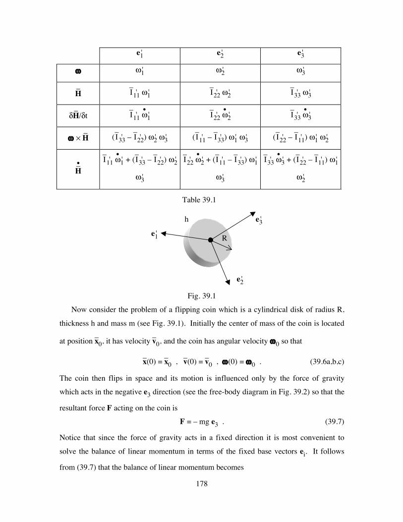
178
e1' e2' e3'
ω ω1' ω2' ω3'
–H –I11' ω1'
–I22' ω2' –I33' ω3'
δ–H/δt
–I11' •ω1'
–I22' •ω2'
–I33' •ω3'
ω × –H (–I33' – –I22' ) ω2' ω3' (–I11' – –I33' ) ω1' ω3' (–I22' – –I11' ) ω1' ω2'
•–H
–I11' •ω1' + (–I33' – –I22' ) ω2'
ω3'
–I22' •ω2' + (–I11' – –I33' ) ω1'
ω3'
–I33' •ω3' + (–I22' – –I11' ) ω1'
ω2'
Table 39.1
Fig. 39.1
Now consider the problem of a flipping coin which is a cylindrical disk of radius R,
thickness h and mass m (see Fig. 39.1). Initially the center of mass of the coin is located
at position –x0, it has velocity –v0, and the coin has angular velocity ω0 so that
–x(0) = –x0 , –v(0) = –v0 , ω(0) = ω0 . (39.6a,b,c)
The coin then flips in space and its motion is influenced only by the force of gravity
which acts in the negative e3 direction (see the free-body diagram in Fig. 39.2) so that the
resultant force F acting on the coin is
F = – mg e3 . (39.7)
Notice that since the force of gravity acts in a fixed direction it is most convenient to
solve the balance of linear momentum in terms of the fixed base vectors ei. It follows
from (39.7) that the balance of linear momentum becomes
e2'
h
R e1'
e3'

179
m ••–x = – mg e3 . (39.8)
Integrating (39.8) subject to the initial conditions (39.6) we deduce that
–x(t) = –x0 + –v0t – 12 g t2 e3 , (39.9)
which shows that the center of mass of the coin moves in a plane parallel to the –v 0–e3
plane.
Fig. 39.2
Taking e3' to be parallel to the axis of revolution of the coin, the components –Iij' of the
inertia tensor –I about the center of mass of the coin are
–Iij' = ⎝⎜⎜⎛
⎠⎟⎟⎞I1 0 0
0 I1 00 0 I3
, I1 = 12 mR2 [1
2 + h2
6R2] , I3 = 12 mR2 . (39.10)
Since the coin is free from moments ( –Mi' = 0), the Euler equations (39.5) reduce to
I1•ω1' + (I3–I1) ω2' ω3' = 0 , (39.11a)
I1 •ω2' – (I3–I1) ω1' ω3' = 0 , (39.11b)
•ω3' = 0 . (39.11c)
Integrating (39.11c) subject to the initial condition (39.6c) we have
ω3' = ω03' = ω0 • e3' (0) = constant , (39.12)
where we emphasize that the components ω0i' are the components of the vector ω0 in the
direction of the base vectors ei'(0) at time t=0 so that
e1 e2
e3
mg

180
ω0i' = ω0 • ei'(0) . (39.13)
Now the equations (39.11a,b) may be rewritten in the simpler forms
•ω1' + λ ω2' = 0 , •
ω2' – λ ω1' = 0 , (39.14a,b)
where the constant λ is defined by
λ = (I3–I1)
I1 ω03' . (39.15)
Differentiating (39.14a) and substituting (39.14b) into the result we deduce that
••ω1' + λ •
ω2' = ••ω1' + λ2 ω1' = 0 . (39.16)
Thus, the solution of (39.16) and hence (39.14b) may be written in the forms
ω1' = ω01' cos(λt) – ω02' sin(λt) , ω2' = ω01' sin(λt) + ω02' cos(λt), (39.17a,b)
where the constants have been determined by satisfying the initial conditions (39.13).
Next, it is convenient to introduce the base vectors ei'' such that
e1'' = cos(λt) e1' + sin(λt) e2' , e2'' = – sin(λt) e1' + cos(λt) e2' , e3'' = e3' ,
ω = ωi' ei' = ω01' e1'' + ω02' e2'' + ω03' e3'' ,
•ei'' = λ × ei'' , λ = ω + λ e3'' = ω01' e1'' + ω02' e2'' + I3I1
ω03' e3'' . (39.18)
However, since the components of λ are constants
•λ =
δλδt + λ × λ = 0 , (39.19)
λ is a constant vector which can be written in the form
λ = •ψ e , •
ψ = α |λ | , e = αλ|λ | , α = 1 for ω03' > 0 and α = – 1 for ω03' < 0 , (39.20)
It then follows that the motion of the coin can be described like a spinning top with the
rate of precession •ψ about the fixed e axis, with spin rate (–λ) (relative to the ei'' axes)
about e3'', and with constant angle of nutation θ given by
cosθ = e3'' • e . (39.21)

181
Moreover, using the fact that the components of –I relative to ei' and ei'' are the same it
follows that the angular momentum about the center of mass
–H = –Iij'' ω j'' ei'' = I1[ω01' e1'' + ω02' e2''] + I3 [ω03' e3''] ,
–H = I1[λ – I3I1
ω03' e3''] + I3 [ω03' e3''] = I1 λ , (39.22)
is a constant vector. This is consistent with the fact that –M vanishes.
Fig. 39.3
θ
•ψ
e – λ e3''